Cost-Benefit Analysis 8.4 Conclusion 8.3 Putting It All Together 8.2 Measuring the Benefits of Public Projects 8.1 Measuring the Costs of Public Projects

Cost-Benefit Analysis

8.4 Conclusion

8.3 Putting It All Together

8.2 Measuring the Benefits of Public Projects

8.1 Measuring the Costs of Public Projects

Chapter 8

cost-benefit analysis The comparison of costs and benefits of public goods projects to decide if they should be undertaken.

Cost-Benefit Analysis: Introduction

Cost-Benefit Analysis is a practical technique for determining the relative merits of alternative government projects over time.

The government uses cost-benefit analysis to compare the costs and benefits of public goods projects and decide if they should be undertaken.

Essentially 3 steps:1. Enumerate all costs and benefits of proposed

project2. Evaluate all costs and benefits in dollar terms3. Discount future net benefits

Introduction

In principle, such an analysis is an accounting exercise. (tracking cost expenditures and benefits)

In practice, cost-benefit analyses are rich economic exercises that combine theory and empirical work.

Example #1

Consider the monorail project in Seattle, which was narrowly approved in 2002. The costs consisted of construction and equipment,

buying permission from some landowners, ruined views, noise near the train, and traffic delays during construction.

The benefits consisted of reduced travel time, saved parking fees, reduced car maintenance, more reliable commuting times, fewer accidents and fatalities, better views for monorail passengers, and reduced noise from busses.

Analysts found that the monorail’s benefits were about $2.07 billion, while its costs were $1.68 billion.

The $390 million net benefit helped swing public opinion toward the project.

MEASURING THE COSTS OF PUBLIC PROJECTS:

Transportation Example Consider the example of renovating a

turnpike that is in poor shape, with large potholes and crumbling shoulders that slow down traffic and pose an accident risk.

Should you repair the road? Table 1Table 1 shows the factors to consider.

Control-Benefit Analysis of Highway Construction Project

Quantity Price or Value

Total

Cost Asphalt 1 million bags

Labor 1 million hours

Maintenance $10 million/year

First-year cost:

Total cost over time:

Benefits

Driving time speed

500,000 hours

Lives saved 5 lives

First-year benefit:

Total benefit over time:

Benefit over time minus cost over time:

Table 1

Valuing Public Benefits and Costs

For private company: Benefits = revenues received Costs = firm’s payments for inputs

For public sector, market prices may not reflect social benefits and costs. Externalities, for example

Several ways of measuring benefits and costs Market prices Adjusted market prices Consumer surplus Inferences from economic behavior Valuing intangibles

Measuring Current Costs

The first goal is to measure current costs. The cash-flow accounting approach to costs simply adds up what the government pays for all the inputs.

This does not represent the social marginal cost we used in the theoretical public goods analysis, however.


The social marginal cost of any resource is its opportunity cost–the value of that input in its next best use. This is not necessarily its cash costs, but

by what else society could do with the input.

For the asphalt, the next best use is to sell the bag to someone else. The value of the alternative use is the market price.


If the labor market is perfectly competitive, the same logic applies–the value of an hour of labor used on the project is simply the market wage.

If there are imperfect markets, however, then there could be unemployment. For example, there could be a “living wage”

ordinance that mandates a $20/hour wage rate. This mandate, in turn, could lead to

unemployment. Imagine that those who were involuntarily

unemployed had a reservation wage of $5/hour; thus, they value their leisure at $5/hour.


In this case, the “alternative activity” is not working at another job, but rather being unemployed. This alternative activity only has an

opportunity cost of $5/hour, not $20/hour. This lowers the economic costs of the

project (but not the accounting costs). The unemployed workers derive rents,

which are simply payments to resource deliverers that exceed those necessary to employ the resource.

The Table 2Table 2 illustrates this.



Total

Cost Asphalt 1 million bags $100/bag $100.0 m


½ at $20/hr½ at $5/hr

$12.5 m


First-year cost:

Total cost over time:

Benefits

Driving time speed

500,000 hours

Lives saved 5 lives

First-year benefit:



Table 2

The accounting cost equals $20/hour x 1 million hours, or $20 million.

Measuring Future Costs

The asphalt and labor costs are immediate costs, but the last one–maintenance–is a stream of costs over time.

This cost is $10 million per year into the indefinite future. We translate this into current dollars using present discounted value.

Present Value:Future Dollars into the Present

Suppose someone promises to pay you $100 one year from now.

What is the maximum amount you should be willing to pay today for such a promise?

You are forgoing the interest that you could earn on the money that is being loaned.


The present value of a future amount of money is the maximum amount you would be willing to pay today for the right to receive the money in the future.

Present Value:Present Dollars into the Future

Define R = amount to be received in future r = rate of return on investment T = years of investment

The present value (PV) of the investment is:

PV

R

rT

1


In previous equation, r is often referred to as the discount rate, and (1+r)-T is the discount factor.

Finally, consider a promise to pay a stream of money, $R0 today, $R1 one year from now, and so on, for T years.

PV R

R

r

R

r

R

rT

T

01 2

21 1 1. . .


Present value is an enormously important concept

A $1,000,000 payment 20 years from now is only worth today: $376,889 if r=.05 $148,644 if r=.10


The key question then becomes choosing the right social discount rate.

For a private firm, the answer would be the opportunity cost of what else the firm could do with the same funds, that is, the after tax rate of return.

The government should base its discount rate on the private sector opportunity cost, but the government counts both the after-tax portion of the return and the taxes collected.


In practice a variety of discount rates are used.

The Office of Management and Budget (OMB) recommended in 1992 that the government use a discount rate of 7%, the historical pre-tax rate of return on private investments, for all public investment projects.

Table 3Table 3 shows the costs.

Table 1. Discount rates used in different government agencies

American Government agencies and organisations

Office of Management and Budget 7%

Bureau of Land Management 10%

U.S. Fish and Wildlife Service 7.8% (nominal rate)

U.S. Forest Service 4%

Congressional Budget Office 2%

Government Accounting Office The average cost of Treasury debt

Municipal Governments 3%



Total



½ at $20/hr½ at $5/hr

$12.5 m


7% disc. rate

$143.0 m

First-year cost: $112.5 m

Total cost over time: $255.5 m

Benefits

Driving time speed

500,000 hours

Lives saved 5 lives

First-year benefit:



Table 3

MEASURING THE BENEFITS OF PUBLIC PROJECTS

There are three main benefits from the project: Value of driving time saved Value of reduced fatalities Value of reduced accidents

Valuing Driving Time Saved For consumers, we need some measure

of society’s valuation of time. There are several approaches to measuring this: Market based measures: Wages Survey based measures: Contingent

valuation Revealed preference measures

Valuing Driving Time Saved

How do we compute the value of commuting time saved?

For producers, the decreased costs shift the supply curve to the right (outward), leading to an increase in the total surplus. Assuming we have estimates of supply and demand in the output market, this is straightforward.


If we had a perfectly functioning labor market, we could “cash out” the value of the time savings, a market-based measure.

Assuming the person can freely choose the hours he wants to work, then even if the time is spent on leisure, the appropriate valuation of the time is the wage rate.

The market based approach runs into problems that hours of work is “lumpy” and that there are non-monetary aspects of the job.


Contingent valuation is a method of asking individuals to value an option they are not now choosing.

In some circumstances, this is the only feasible method for valuing a public good. For example, there is no obvious market

price to use to value saving a rare species of owl.

Problems with contingent Problems with contingent valuationvaluation

There are serious issues with contingent valuation, however. Isolation of issues matter: respondents value a

public good more when it is the only one asked about.

Order of issues matter: respondents place higher values on public goods asked about first.

“Embedding” matters: respondents seem to place roughly the same valuation on a public good, regardless of the quantity.

These problems suggest that part of the valuation is due to survey design, not “true” valuation.

Applicati

Applicati

onon


The natural way for economists to value time is to use revealed preference–let the actions of individuals reveal their valuation.

For example, if one compared house prices for two houses, one of which was 5 minutes closer to the workplace, this would effectively “cash out” the value of saved commuting time.


In practice, this approach runs into problems because the two homes are not identical.

Some of the differences (e.g., housing attributes) can be observed and accounted for with cross sectional regression. Decomposing a sale price by its attributes is the basis of hedonic market analysis.

Other differences are either hard to measure or unobserved, however, which leads to bias.

Valuing time savingsValuing time savings

One clever quasi-experiment to reveal the value of saved time was conducted by Deacon and Sonstelie (1985): During the oil crisis of the 1970s, the government

imposed price ceilings on gasoline of large gasoline stations, but not independent ones.

As a consequence, long lines formed at these cheaper, corporate gasoline stations.

At Chevron stations in California, gasoline was approximately 39.5¢ lower, with an average wait time of roughly 14.6 minutes. The mean purchase was around 10.5 gallons.

Thus, the tradeoff is waiting 14.6 minutes to save about $4.15, or one hour for $17. This corresponded very closely to the average hourly wage in the U.S.

Empirical

Empirical

EvidenEviden

cece

Valuing Saved Lives

The other main benefit of the turnpike improvement is valuing saved lives due to lower traffic fatalities.

Valuing life runs into ethical issues, but almost all economists would agree that it is necessary for public policy decisions.

Valuing Saved Lives

By stating that life is priceless or should not be valued, we leave ourselves helpless when facing choices of different programs that could each save lives.

There are three main approaches to doing this: Using wages Contingent valuation Revealed preference

Valuing Public Benefits and Costs

Economists use two methods to assign finite values to human life: Lost earnings: Net present value of individual’s

after-tax earnings over lifetime. Taken literally, no loss for aged, infirm, or severely

handicapped Probability of death: Most projects affect probability

of death (e.g., cancer research). People are willing to accept increases in the probability of death for a finite amount of money.

Valuing lifeValuing life

In 1993, consumer groups demanded that General Motors recall 5 million pickup trucks. The trucks’ side-mounted gas tanks made

them more likely to explode on impact, causing 150 deaths over a 15-year period.

The recall would cost $1 billion, and save at most 32 more lives, or $31.25 million per life saved.

GM reached a rather different settlement–provide $50 million for education about seat belts and drunk driving, and provide 200,000 child safety seats for low-income families.

Applicati

Applicati

onon

Valuing lifeValuing life

The settlement was called “the most unprecedented buyout of law enforcement officials by a culpable corporation in regulation history.” – Ralph Nader.

Yet, the child safety seats alone would save 50 lives, which at a cost of $50 million, leads to a cost per life saved of just $1 million. Far more cost effective than the $31.25

million per life saved from the recall. Thus, by this measure, the settlement was

much better, but only possible because the government “valued life.”

Applicati

Applicati

onon

Valuing Saved Lives

The market-based approach uses wages; the value of the life is the present discounted value of the lifetime stream of earnings.

One key problem is that this approach does not value leisure. Keeler (2001) suggests that because of this, the value of a person’s life is about 5 to 10 times their future lifetime earnings.

Valuing Saved Lives

Keeler finds that the average 20 year-old female will have future earnings of $487,000 in net present value, but will value her life at $3.1 million.

Men have slightly higher values because of higher earnings.

Older people have lower values because they have fewer years of life remaining.

Valuing Saved Lives

The contingent valuation approach asks about the valuation of a life

There is obvious difficulty in a question like this, so it is often framed in terms of changes in the probability of dying. For example, how much more would you

pay for an airline ticket with a 1 in 500,000 chance of a crash compared with a 2 in 500,000 chance?

The estimates from contingent valuation have a very wide range, going from $825,000 to $22.3 million per life saved.

Valuing Saved Lives

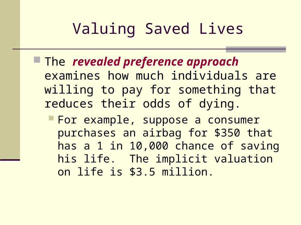
The revealed preference approach examines how much individuals are willing to pay for something that reduces their odds of dying. For example, suppose a consumer

purchases an airbag for $350 that has a 1 in 10,000 chance of saving his life. The implicit valuation on life is $3.5 million.

Valuing Saved Lives

An alternative revealed preference approach examines risky jobs: Suppose that one job has a 2% higher

risk of death but pays $15,000 more in salary.

The $15,000 extra salary is known as the compensating differential.

The implicit valuation of life in this example is $3 million ($15,000/0.02).

Valuing Saved Lives

There is a large literature in economics using these revealed preference approaches. Viscusi estimates that the value of life is roughly $7 million.

There are drawbacks, however. Strong information assumptions about

probabilities. Assumes people are well prepared to evaluate

these tradeoffs. Difficult to control for other attributes of the job. Differences in valuation of life (e.g., degree of

risk aversion).

www.law.georgetown.edu/gelpi/papers/pricefnl.pdf

CBA Criticisms

Applications to health and environmental safety is flawed because of difficulty measuring non market items

Substituting risk of death with death is wrong CBA ignores who suffers from an

environmental or health risk problem

Valuing Saved Lives

Another approach focuses on how existing government spending translates into lives saved.

Recent study reviewed 76 regulatory programs; the costs per saved live varied between $100,000 for childproof cigarette lighters to $100 billion from regulation of solid waste disposal facilities.

Table 4 Table 4 shows the results.

Table 4

Costs Per Life Saved of Various Regulations

Regulation concerning … Year Agency

Cost per life saved

($ millions)

Childproof lighters 1993 CPSC $0.1

Food labeling 1993 FDA 0.4

Reflective devices for heavy trucks

1999 NHTSA 0.9

Children’s sleepware flammability

1973 CPSC 2.2

Rear/up/should seatbelts in cars

1989 NHTSA 4.4

Asbestos 1972 OSHA 5.5

Value of statistical life 7.0

Benezene 1987 OSHA 22

Asbestos ban 1989 EPA 78

Cattle feed 1979 FDA 170

Solid waste disposal facilities 1991 EPA 100,000

Discounting Future Benefits

A particularly thorny issue for cost-benefit analysis is that the costs are mostly short-term, while the benefits are mostly long term. Global warming is a good example.

This may be problematic because: The choice of discount rate will matter

enormously for benefits that are far in the future.

The benefits are spread out over current and future generations.

Cost-effectiveness Analysis

Finally, there may be cases when society is unwilling or unable to value the benefits of a public project.

Cost-effectiveness analysis is the search for the most cost-effective approach to providing a public good, ignoring whether the benefits warrant such a public good.

PUTTING IT ALL TOGETHER

Table 5Table 5 adds in the benefits from the turnpike renovation.



Total



½ at $20/hr½ at $5/hr

$12.5 m


7% disc. rate

$143.0 m

First-year cost: $112.5 m

Total cost over time: $255.5 m

Benefits

Driving time speed

500,000 hours $17/hr $8.5 m

Lives saved 5 lives $7 million/life

$35.0 m

First-year benefit: $43.5 m

Total benefit over time: $621.4 m


$365.9 m

Table 5

NPV: B – C = $255.5 M

B/C ratio: 1.698

PUTTING IT ALL TOGETHER

Since the benefits exceed the costs, we would recommend the government pursue the project.

The government needs to consider one additional factor beyond the benefits and costs of the project itself: the budgetary cost of raising the funds to finance the project.

Economists typically assume some efficiency cost, or deadweight loss, from raising the tax burden to finance this spending. If the efficiency cost of raising the money is too high, some projects will not survive the cost-benefit analysis.

Private Sector Project Evaluation

The present value criteria for project evaluation are that: A project is admissible only if its present

value is positive. When two projects are mutually exclusive,

the preferred project is the one with the highest present value.


Table 11.2 shows two different projects (R&D or Advertising).

The discount rate plays a key role in deciding what project to choose, because the cash inflows occur at different times.

The lower the discount rate, the more valuable the back-loaded project.

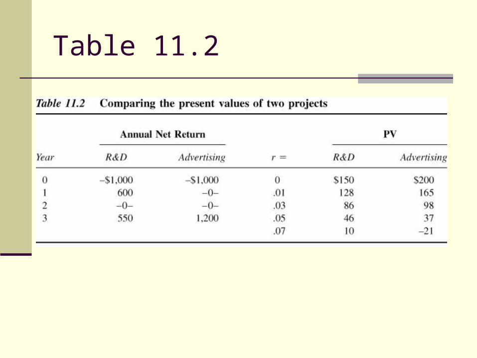
Table 11.2


Several other criteria are often used for project evaluation, but can give misleading answers Internal rate of return Benefit-cost ratio


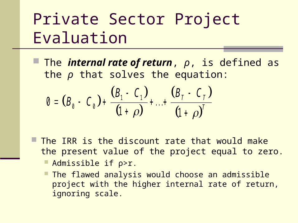
The internal rate of return, ρ, is defined as the ρ that solves the equation:

01 1

0 01 1

B C

B C B CT TT

. . .

The IRR is the discount rate that would make the present value of the project equal to zero. Admissible if ρ>r. The flawed analysis would choose an admissible project

with the higher internal rate of return, ignoring scale.


The benefit-cost ratio divides the discounted stream of benefits by the discounted stream of costs. In this case:B=stream of benefits and C=stream of costs:

B B

B

r

B

rT

T

01

1 1. . .

C C

C

r

C

rT

T

01

1 1. . .


Admissibility using the benefit-cost ratio requires:

B

C1

This ratio is virtually useless for comparing across admissible projects, however.

Ratio can be manipulated by counting benefits as “negative costs” and vice-versa.

Discount Rate for Government Projects

Government decision making involves present value calculations.

Costs, benefits, and discount rates are somewhat different from private sector.

Valuing Public Benefits and Costs: other considerations

Consumer surplus Public sector projects can be large and

change market prices. Figure 11.1 measures the change in

consumer surplus from a government irrigation project that lowers the cost of agricultural production.

Figure 11.1

Other Issues in Cost-Benefit Analysis

There are a number of other issues in cost-benefit analysis.

These concern common “counting” mistakes and distributional concerns.


The common counting mistakes or “games” include: Counting secondary benefits (like commerce that

is simply shifted from one area to another). Counting labor as a benefit rather than a cost. Double counting benefits (like the value of an

irrigation project to farm income, and simultaneously the increase in the value of the land)

Chain-Reaction game: Include secondary benefits to make a proposal appear more favorable, without also including the secondary costs

.


There are also distributional concerns: The costs and benefits of a public

project do not necessarily accrue to the same individuals.

In principle, a project that improved social welfare could then involve redistribution, but in practice this rarely happens.

Budgetary Costs

Although we would recommend that the government pursue this project because the benefits were greater than the costs, in reality governments face limited budgets.

To assess which of many projects to pursue, the government must consider the budgetary cost of raising funds to finance the project. This involves some efficiency costs, or

deadweight loss. This cost should be factored into the

calculations.

Budgetary Costs

For example, consider two projects that pass the cost-benefit test: One project has benefits of $150, and

costs $100. The other has benefits of $110, and

costs $100. If the efficiency costs of raising funds is

20¢ for each $1 of revenue raised, then only the first project (with benefits that exceed $120) should be pursued.

Recap of Cost-Benefit Analysis

Measuring the costs of public projects Measuring the benefits of public

projects Putting it all together

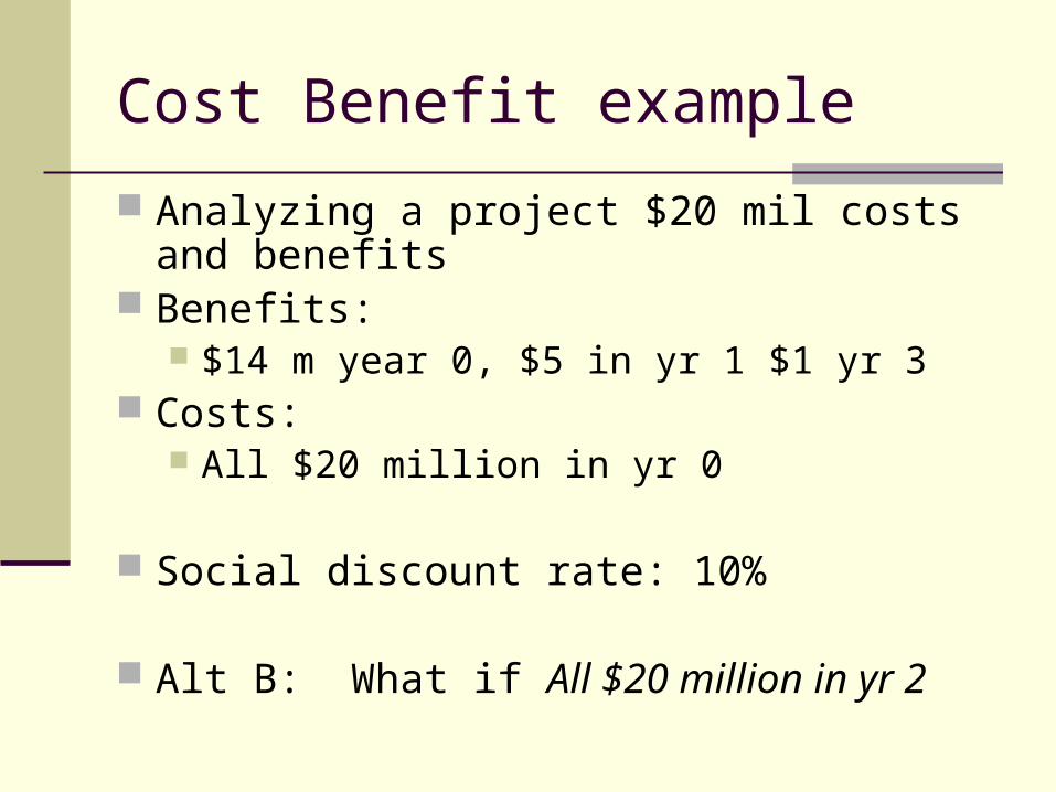
Cost Benefit example

Analyzing a project $20 mil costs and benefits Benefits:

$14 m year 0, $5 in yr 1 $1 yr 3 Costs:

All $20 million in yr 0

Social discount rate: 10%

Alt B: What if All $20 million in yr 2

Documents

Cost-Benefit Analysis 8.4 Conclusion 8.3 Putting It All Together 8.2 Measuring the Benefits of Public Projects 8.1 Measuring the Costs of Public Projects