Cost effective combined axial fan and throttling valve

control of ventilation rate

C.J. Taylor 1

P.A. Leigh, A. Chotai, P.C. Young 2

E. Vranken, D. Berckmans 3

This paper is a postprint of a paper submitted to and accepted for

publication in IEE Proceedings Control Theory and Applications and is

subject to Institution of Engineering and Technology Copyright. The copy

of record is available at IET Digital Library. [IEE Proceedings Control

Theory and Applications 151, 5, 577–584, 2004]

1Engineering Department, Lancaster University, Lancaster, LA1 4YR, UK

2Department of Environmental Science, Lancaster University, UK

3Lab. for Agricultural Buildings Research, Katholieke Universiteit Leuven, Belgium

1

Abstract

This paper is concerned with Proportional-Integral-Plus (PIP) control of

ventilation rate in mechanically ventilated agricultural buildings. In partic-

ular, it develops a unique fan and throttling valve control system for a 22m3

test chamber, representing a section of a livestock building or glasshouse, at

the Katholieke Universiteit Leuven. Here, the throttling valve is employed

to restrict airflow at the outlet, so generating a higher static pressure differ-

ence over the control fan. In contrast with previous approaches, however, the

throttling valve is directly employed as a second control actuator, utilising

airflow from either the axial fan or natural ventilation. The new combined

fan/valve configuration is compared with a commercially available PID-based

controller and a previously developed scheduled PIP design, yielding a re-

duction in power consumption in both cases of up to 45%.

Keywords

Agriculture; identification; control system design; model-based control; PIP

control; PID control

2

1 Introduction

Ventilation rate is one of the most significant inputs in the control of mi-

croclimate surrounding plants or animals within the majority of agricultural

buildings, including livestock housing, glasshouses and storage warehouses;

see e.g. [1, 2, 3, 4]. For example, without adequate fresh air supply within

a livestock enclosure, animal comfort and welfare are drastically reduced,

especially during high density occupation by poultry, pigs or cattle, where

excessive levels of moisture, heat and internal gases are generated. For this

reason, the lack of effective ventilation rate control is a major cause of pro-

duction losses and health problems in modern livestock buildings.

To date, the most common type of controllers used in agricultural build-

ings are derived from the ubiquitous Proportional-Integral-Derivative (PID)

algorithms; e.g. [5, 6]. In this regard, the Proportional-Integral-Plus (PIP)

controller considered in the present paper, can itself be interpreted as a logical

extension of conventional PI/PID controllers, but with inherent model-based

predictive control action [7]. Here, a Non-Minimal State Space (NMSS)

model is formulated so that full state variable feedback control can be imple-

mented directly from the measured input and output signals of the controlled

process, without resort to the design and implementation of a deterministic

state reconstructor or a stochastic Kalman filter [8]. Such PIP control sys-

3

tems have been successfully implemented in a wide range of applications,

including the control of ventilation rate in a 22m3 laboratory test installa-

tion at the Katholieke Universiteit Leuven [9, 10].

In the latter regard, it should be noted that the desired airflow rate

within agricultural buildings is typically set at a relatively low level. It

is reasonably straightforward to maintain these low airflow rates (even in

open loop) when the system is undisturbed. In practice, however, pressure

disturbances caused by variations in wind speed outside the building, coupled

with eddy currents or thermals inside, have a significant influence on the

ventilation rate produced by an axial fan. In fact, at low ventilation rates,

the air velocity vectors in the neighbourhood of the fan can be very turbulent,

resulting in a fluctuating ventilation rate that is unsuitable for maintaining

the environmental requirements (temperature, humidity, gas concentration)

and the welfare of the animals within the building.

For this reason, a throttling valve has been developed to provide a second

control actuator to the Leuven test chamber, as illustrated in Fig. 1. The

radial blades of this valve (or vortex damper) can rotate through 90 degrees.

At low ventilation rates, the valve is employed to restrict airflow through the

chamber, so generating a higher static pressure difference over the control fan.

For example, [10] consider the design and implementation of a gain scheduled

PIP algorithm that activates the throttling valve when the ventilation rate

4

falls below 1000m3/h. For this preliminary design, the valve is always closed

by a predetermined amount (60%) in order to help stabilise the airflow. The

approach yields good control over a wide range of operating conditions when

compared with a commercially available PID design. Of course, when the

PIP or PID algorithms restrict the airflow in this way, the axial fan inevitably

consumes more power in order to maintain a given ventilation rate.

By contrast, the present paper develops a PIP algorithm for active control

of the throttling valve itself. Here, on-line adjustments are made to the blade

angle at each control sample, in order to directly regulate the ventilation rate.

The necessary airflow is generated either by the PIP controlled axial fan or,

where appropriate, by natural ventilation caused by temperature gradients

and wind outside the building. A simple rule-based algorithm switches con-

trol back to the fan when the throttling valve is no longer effective.

Following a brief description of the test chamber in Section 2, the mod-

elling and control methodologies are developed in Sections 3 and 4 respec-

tively. In Section 5, the new fan and throttling valve configuration is com-

pared with previously developed controllers that use the same control ac-

tuators. Since microclimate control typically amounts to circa 15% of the

production costs [4], the study pays particular attention to the relative power

consumption of the various algorithms. Finally, the conclusions are given in

Section 6.

5

2 Experimental chamber

The research discussed here is based on data collected from an instrumented

ventilation test chamber at the Laboratory for Agricultural Buildings Re-

search of the Katholieke Universiteit Leuven (Fig. 1). This facility has been

designed to represent a section of a livestock building or glasshouse. Air is

extracted from the chamber by an axial fan (diameter 0.45m), while a venti-

lation rate sensor (certified accuracy 50m3/h) is used for continuous feedback

control.

A throttling valve alongside the ventilation rate sensor is utilised to re-

strict outflow. The radial blades can rotate from 0 to 90 degrees, i.e. ranging

between perpendicular (fully closed) and parallel (fully open) to airflow di-

rection. The power consumption of the throttling valve is insignificant in

comparison to the fan. At the other side of the pressure chamber a second

fan is used to create a dynamic pressure difference over the pressure chamber,

thus simulating wind disturbances and natural ventilation.

Although not required for on-line control, static pressure differences over

the control fan are measured with a differential pressure sensor that is au-

tomatically calibrated at the start of each experiment against a reference

pressure sensor. Such measurements are particularly useful when specifying

an appropriate signal to the disturbance fan in order to compare different

6

control strategies. Here, the voltage applied to the disturbance fan is ad-

justed by trial and error in a series of open loop experiments, in order to

match the pressure differences observed on the external walls of a real build-

ing. As discussed in more detail by [4], this allows a realistic disturbance

fan signal to be obtained from wind speed measurements. The present study

utilises wind and pressure data collected at Silsoe Research Institute on a

windy day with a mean wind speed of 4m/s [11].

The disturbance fan can also be utilised to represent any natural ventila-

tion present in the system. Convenience and cost factors ensure that many

farms install fans into the sidewall. This is a prominent feature of livestock

farming in the low countries of Europe, including Belgium and Holland, where

numerous farms are built along the coast of the North Sea and so are sub-

jected to strong prevailing westerly winds. Furthermore, the ‘chimney effect’

tends to produce natural ventilation, especially when there is a temperature

difference between inside and outside the building. In the latter case, warm

air will be drawn from the interior towards any chimney structure, setting

up a natural air-circulation without an electro/mechanical fan to drive it. In

the case of the test chamber, the disturbance fan provides an airflow that is

similarly independent of the main (control) fan.

7

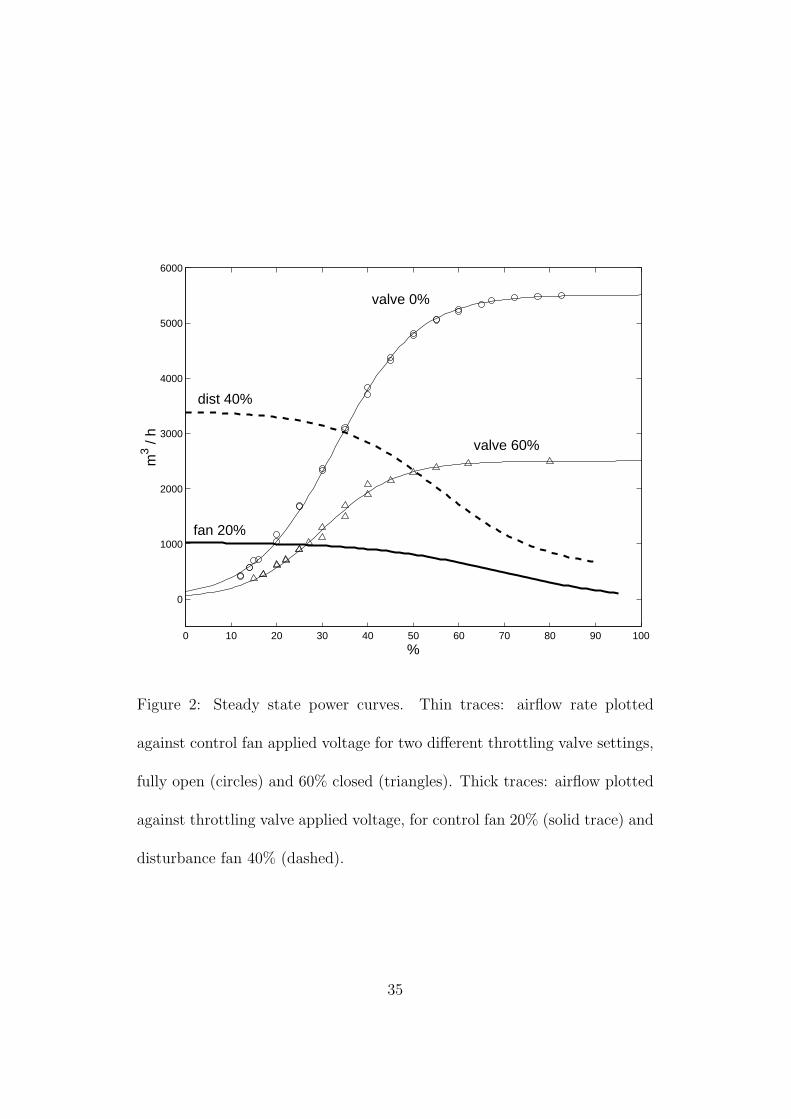
2.1 Power curves

The steady state relationship between airflow rate and the potential voltage

applied to the control fan is illustrated in Fig. 2 (circles), which takes the

form of a conventional non-linear ‘S’ shaped curve. Here, a flexible logistic

growth function has been numerically fitted to the data (in a least squares

sense) in order to better highlight the relationship between these variables.

It should be pointed out that no airflow is produced below a certain

potential voltage due to the motor characteristics of the fan, i.e. a certain

threshold voltage is required to start the blades turning. In both Fig. 2

and the later analysis, the voltage is expressed as a percentage, where 0%

represents this threshold and 100% is the maximum voltage normally applied.

The triangular data points in Fig. 2 are obtained for a partially closed

throttling valve, illustrating the reduced ventilation rates when compared to

the fully open valve case, for a given control fan setting. Here, the applied

input to the throttling valve similarly ranges from 0% (valve fully open)

to 100% (fully closed). In the case of the triangular data data points, the

throttling valve input is 60%. It is clear from Fig. 2 that closing the valve

increases operating costs for the control fan, since a higher voltage is required

to maintain a given airflow.

Finally, the solid and dashed thick traces in Fig. 2 are for logistic growth

8

functions fitted to the steady state relationship between airflow rate and the

applied voltage to the throttling valve. For the dashed trace, the control

fan is turned off and the airflow is entirely provided by the disturbance fan

operating at 40% power. For example, with the throttling valve blades turned

parallel to the airflow, the mean ventilation rate is 3380m3/h. The solid trace

is obtained with the disturbance fan turned off and 20% voltage applied to

the control fan, yielding ventilation rates up to 1000m3/h.

These power curves suggest that, for a potential airflow generated by

either the axial fan or an external disturbance, the ventilation rate may be

regulated (reduced) by adjustment of the throttling valve. Of course, the

set point reachable in such cases is constrained by the external force driving

the airflow. In this regard, note that when the voltage applied to the valve

exceeds ≈ 95%, the airflow sometimes becomes unstable because the outlet

from the chamber is almost entirely blocked, hence the power curves are not

graphed beyond this point.

3 System identification and estimation

In order to develop a PIP control algorithm, a linearised representation of the

system is required. Even for non-linear systems, the essential small perturba-

tion behaviour can usually be approximated well by simple linearised Trans-

9

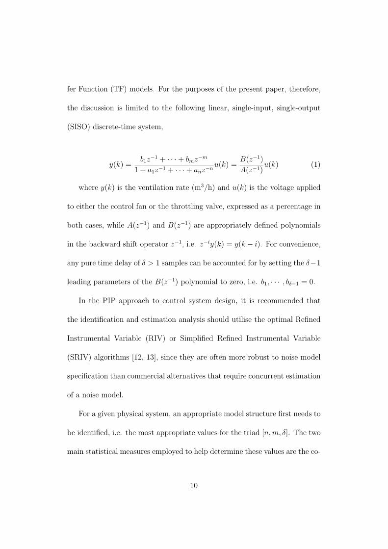
fer Function (TF) models. For the purposes of the present paper, therefore,

the discussion is limited to the following linear, single-input, single-output

(SISO) discrete-time system,

y(k) =b1z

−1 + · · ·+ bmz−m

1 + a1z−1 + · · ·+ anz−nu(k) =

B(z−1)

A(z−1)u(k) (1)

where y(k) is the ventilation rate (m3/h) and u(k) is the voltage applied

to either the control fan or the throttling valve, expressed as a percentage in

both cases, while A(z−1) and B(z−1) are appropriately defined polynomials

in the backward shift operator z−1, i.e. z−iy(k) = y(k− i). For convenience,

any pure time delay of δ > 1 samples can be accounted for by setting the δ−1

leading parameters of the B(z−1) polynomial to zero, i.e. b1, · · · , bδ−1 = 0.

In the PIP approach to control system design, it is recommended that

the identification and estimation analysis should utilise the optimal Refined

Instrumental Variable (RIV) or Simplified Refined Instrumental Variable

(SRIV) algorithms [12, 13], since they are often more robust to noise model

specification than commercial alternatives that require concurrent estimation

of a noise model.

For a given physical system, an appropriate model structure first needs to

be identified, i.e. the most appropriate values for the triad [n,m, δ]. The two

main statistical measures employed to help determine these values are the co-

10

efficient of determination R2T , based on the response error; and YIC (Young’s

Information Criterion), which provides a combined measure of model fit and

parametric efficiency, with large negative values indicating a model which

explains the output data well, without over-parameterisation [13].

An important variable in the recursive estimation equations is the pa-

rameter covariance matrix P∗(k), which is the inverse of the Instrumental

Cross-Product Matrix [see e.g. 14] scaled by the estimated noise variance.

The standard errors on the parameter estimates may be computed from the

diagonal elements of P∗(k). Also, P∗(k) provides an estimate of the un-

certainty associated with the model parameters which can be employed in

subsequent Monte Carlo analysis (see Section 4.5 below).

Finally, note that these statistical tools and associated estimation algo-

rithms have been assembled as the CAPTAIN toolbox within the Matlab R©

software environment (www.es.lancs.ac.uk/cres/captain). The authors can

be contacted for further details about the toolbox.

3.1 Control model for the axial fan

The paper discusses the design of PIP control systems for ventilation rate,

based on a sampling rate of 2 seconds. Experimentation reveals that such

a sampling rate yields a good compromise between a fast response and a

11

desirable low order model and control algorithm.

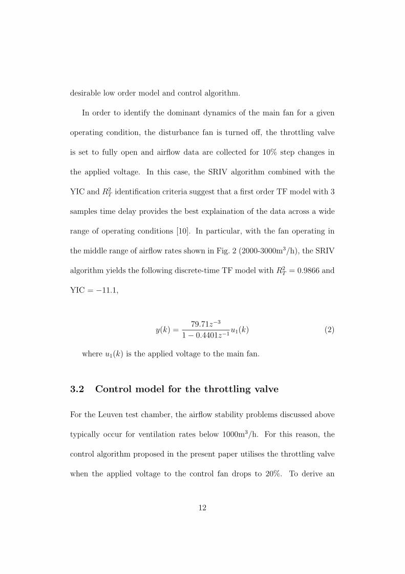
In order to identify the dominant dynamics of the main fan for a given

operating condition, the disturbance fan is turned off, the throttling valve

is set to fully open and airflow data are collected for 10% step changes in

the applied voltage. In this case, the SRIV algorithm combined with the

YIC and R2T identification criteria suggest that a first order TF model with 3

samples time delay provides the best explaination of the data across a wide

range of operating conditions [10]. In particular, with the fan operating in

the middle range of airflow rates shown in Fig. 2 (2000-3000m3/h), the SRIV

algorithm yields the following discrete-time TF model with R2T = 0.9866 and

YIC = −11.1,

y(k) =79.71z−3

1− 0.4401z−1u1(k) (2)

where u1(k) is the applied voltage to the main fan.

3.2 Control model for the throttling valve

For the Leuven test chamber, the airflow stability problems discussed above

typically occur for ventilation rates below 1000m3/h. For this reason, the

control algorithm proposed in the present paper utilises the throttling valve

when the applied voltage to the control fan drops to 20%. To derive an

12

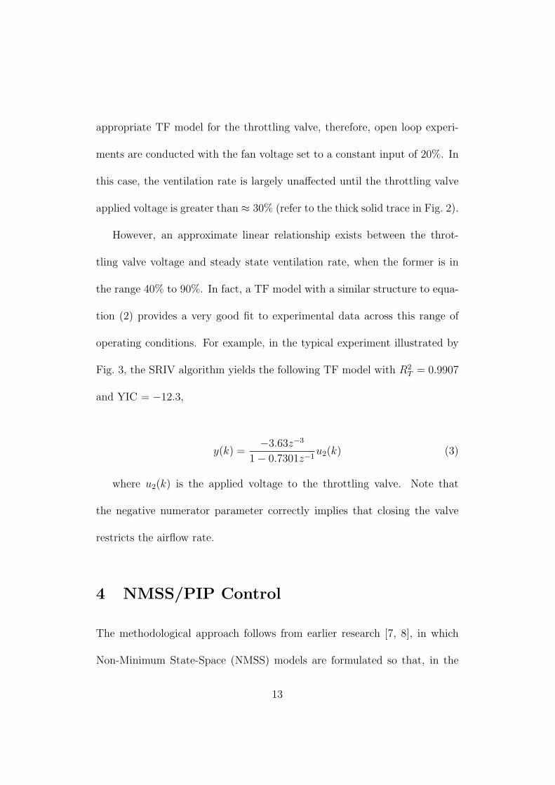
appropriate TF model for the throttling valve, therefore, open loop experi-

ments are conducted with the fan voltage set to a constant input of 20%. In

this case, the ventilation rate is largely unaffected until the throttling valve

applied voltage is greater than ≈ 30% (refer to the thick solid trace in Fig. 2).

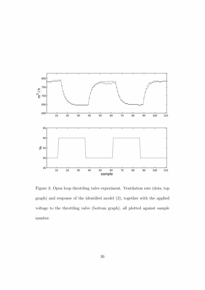
However, an approximate linear relationship exists between the throt-

tling valve voltage and steady state ventilation rate, when the former is in

the range 40% to 90%. In fact, a TF model with a similar structure to equa-

tion (2) provides a very good fit to experimental data across this range of

operating conditions. For example, in the typical experiment illustrated by

Fig. 3, the SRIV algorithm yields the following TF model with R2T = 0.9907

and YIC = −12.3,

y(k) =−3.63z−3

1− 0.7301z−1u2(k) (3)

where u2(k) is the applied voltage to the throttling valve. Note that

the negative numerator parameter correctly implies that closing the valve

restricts the airflow rate.

4 NMSS/PIP Control

The methodological approach follows from earlier research [7, 8], in which

Non-Minimum State-Space (NMSS) models are formulated so that, in the

13

deterministic situation, full state feedback control can be implemented di-

rectly from the measured input and output signals of the controlled process,

without resort to the design and implementation of a state reconstructor

(or observer). As shown below, the approach automatically accomodates the

mutliple-time delays observed in both the throttling valve and axial fan actu-

ators, and yields a Proportional-Integral-Plus (PIP) design that is naturally

robust to uncertainty, eliminating the need for measures such as loop transfer

recovery.

The proposed fan/valve configuration employs independently designed,

single input, single output (SISO) controllers to determine the applied voltage

to the axial fan and the throttling valve. Although the NMSS/PIP methodol-

ogy is straightforwardly extended to multivariable systems [e.g. 15], this has

not proven necessary in the present case. In fact, as discussed in Section 4.6,

simple rules are implemented to switch between the two algorithms.

4.1 Non-Minimal State-Space (NMSS) form

It is easy to show that the model (1) can be represented by the following

NMSS equations,

x(k) = Fx(k − 1) + gu(k − 1) + dyd(k)

y(k) = hx(k)

(4)

14

The n+m dimensional non-minimal state vector x(k), so called because

it is of higher dimension than conventional nth order minimal state vectors,

consists of the present and past sampled values of the output variable y(k)

and the past sampled values of the input variable u(k), i.e.,

x(k) =

[

y(k) y(k − 1) · · · y(k − n+ 1) u(k − 1) u(k −m+ 1) z(k)

]T

(5)

where z(k) is the integral-of-error between the reference or command

input yd(k) and the sampled output y(k), defined as follows,

z(k) = z(k − 1) + yd(k)− y(k) (6)

The state transition matrix F, input vector g, command input vector d

and output vector h of the NMSS system are subsequently defined below,

15

F =

−a1 −a2 · · · −an−1 −an b2 b3 · · · bm−1 bm 0

1 0 · · · 0 0 0 0 · · · 0 0 0

0 1 · · · 0 0 0 0 · · · 0 0 0

......

. . ....

......

.... . .

......

...

0 0 · · · 1 0 0 0 · · · 0 0 0

0 0 · · · 0 0 0 0 · · · 0 0 0

0 0 · · · 0 0 1 0 · · · 0 0 0

0 0 · · · 0 0 0 1 · · · 0 0 0

......

. . ....

......

.... . .

......

...

1 0 · · · 0 0 0 0 · · · 1 0 0

a1 a2 · · · an−1 an −b2 −b3 · · · −bm−1 −bm 1

g =

[

b1 0 0 · · · 0 1 0 0 · · · 0 −b1

]T

d =

[

0 0 0 · · · 0 0 0 0 · · · 0 1

]T

h =

[

1 0 0 · · · 0 0 0 0 · · · 0 0

]T

(7)

Inherent type 1 servomechanism performance is introduced by means of

the integral-of-error part of the state vector, z(k). If the closed-loop system

is stable, then this ensures that steady-state tracking of the command level

is inherent in the basic design.

16

4.2 Proportional-Integral-Plus (PIP) control

The State Variable Feedback (SVF) control law associated with the NMSS

model (4) takes the usual form,

u(k) = −kx(k) (8)

where k is the n+m dimensional SVF control gain vector,

k =

[

f0 f1 · · · fn−1 g1 · · · gm−1 − kI

]

(9)

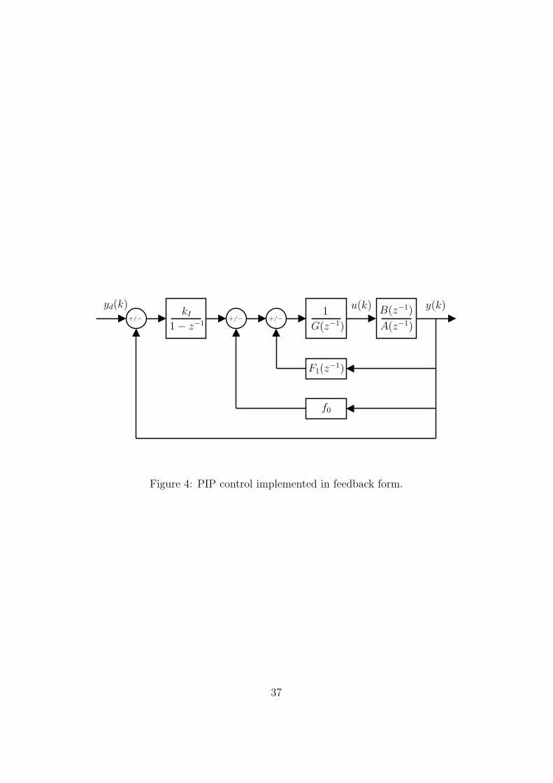
In more conventional block-diagram terms, the SVF controller (8) can be

implemented as shown in Fig. 4, where it is clear that it can be considered

as one particular extension of the ubiquitous PI controller, in which the

PI action is, in general, enhanced by the higher order forward path and

feedback compensators 1/G(z−1) and F1(z−1), respectively, where 1/G(z−1)

and F1(z−1) are defined as follows,

F1(z−1) = f1z

−1 + · · ·+ fn−1z−(n−1)

G(z−1) = 1 + g1z−1 + · · ·+ gm−1z

−(m−1)

(10)

However, because it exploits fully the power of SVF within the NMSS

setting, PIP control is inherently much more flexible and sophisticated, al-

lowing for well-known SVF strategies such as closed loop pole assignment,

17

with complete (or partial) decoupling control in the multivariable case; or

optimisation in terms of a Linear-Quadratic (LQ) cost function of the form,

J =1

2

∞∑

i=0

{

x(i)Qx(i) + ru2(i)}

(11)

where Q is a n+m by n+m matrix and r is a scalar weight on the input.

It is worth noting that, due to the special structure of the non-minimal state

vector, the elements of the LQ weighting matrices have particularly simple

interpretation, since the diagonal elements directly define weights assigned to

the measured variables and integral-of-error states. For example, Q can be

formed conveniently as a diagonal matrix with elements defined as follows,

Q = diag

(

q1 q2 · · · qn qn+1 · · · qn+m−1 qn+m

)

(12)

Here, the user defined output weighting parameters q1, q2, . . . , qn, and

input weighting parameters qn+1, qn+2, . . . , qn+m−1, are generally set equal to

common values of qy and qu respectively; while qn+m is denoted by qe to

indicate that it provides a weighting constraint on the integral-of-error state

variable z(k). In this ‘three term’ formulation (analogous to the conventional

three-term PID controller), the input weight is defined as r = qu.

The ‘default’ PIP-LQ controller is then obtained using total optimal con-

trol weights of unity, i.e., qy = 1/n, qu = 1/m and qe = 1. The resulting SVF

18

gains are obtained from the steady state solution of the well known discrete

time matrix Riccati equation [e.g. 16].

In many cases, good closed loop performance is obtained by straightfor-

ward manual tuning of the diagonal LQ weights as discussed above. Alterna-

tively, in more difficult situations, the PIP control system is ideal for incorpo-

ration within a multi-objective optimisation framework, where satisfactory

compromise can be obtained between conflicting objectives such as robust-

ness, overshoot, rise times and multivariable decoupling. This is achieved

by concurrent optimisation of the diagonal and off diagonal elements of the

weighting matrices in the cost function, as described by [17].

4.3 Incremental form

In practice, the PIP control law derived from Fig. 4 is always implemented

in the following incremental form,

u(k) = u(k − 1) + kI {yd(k)− y(k)} − F (z−1)∆y(k)−{

G(z−1)− 1}

∆u(k)

(13)

where ∆ = 1− z−1 is the difference operator and F (z−1) = f0 + F1(z−1).

Equation (13) is not only the most obvious and convenient for digital imple-

mentation but also provides an inherent means of avoiding ‘integral windup’

19

in the PIP controller. To avoid such integral wind up, which is caused by

integration of control errors during periods of actuator saturation, equation

(13) is employed with the following correction,

u(k) =

umax when u(k) > umax

umin when u(k) < umin

(14)

In this manner, u(k) and its past values are kept within their practically

realisable limits, represented here by umin and umax.

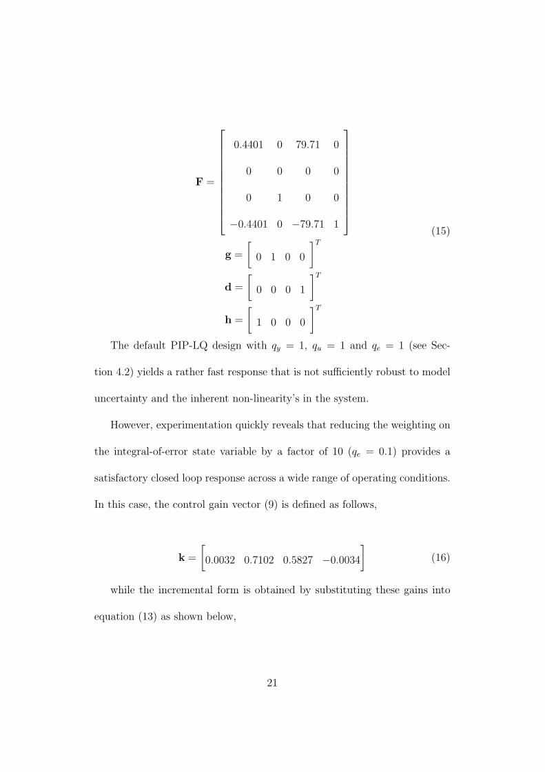
4.4 PIP control design for the axial fan

For the transfer function model (2), the NMSS form (4) is based on the

definition of four state variables, i.e. y(k), u(k − 1), u(k − 2) and z(k). The

state matrices are defined as follows,

20

F =

0.4401 0 79.71 0

0 0 0 0

0 1 0 0

−0.4401 0 −79.71 1

g =

[

0 1 0 0

]T

d =

[

0 0 0 1

]T

h =

[

1 0 0 0

]T

(15)

The default PIP-LQ design with qy = 1, qu = 1 and qe = 1 (see Sec-

tion 4.2) yields a rather fast response that is not sufficiently robust to model

uncertainty and the inherent non-linearity’s in the system.

However, experimentation quickly reveals that reducing the weighting on

the integral-of-error state variable by a factor of 10 (qe = 0.1) provides a

satisfactory closed loop response across a wide range of operating conditions.

In this case, the control gain vector (9) is defined as follows,

k =

[

0.0032 0.7102 0.5827 −0.0034

]

(16)

while the incremental form is obtained by substituting these gains into

equation (13) as shown below,

21

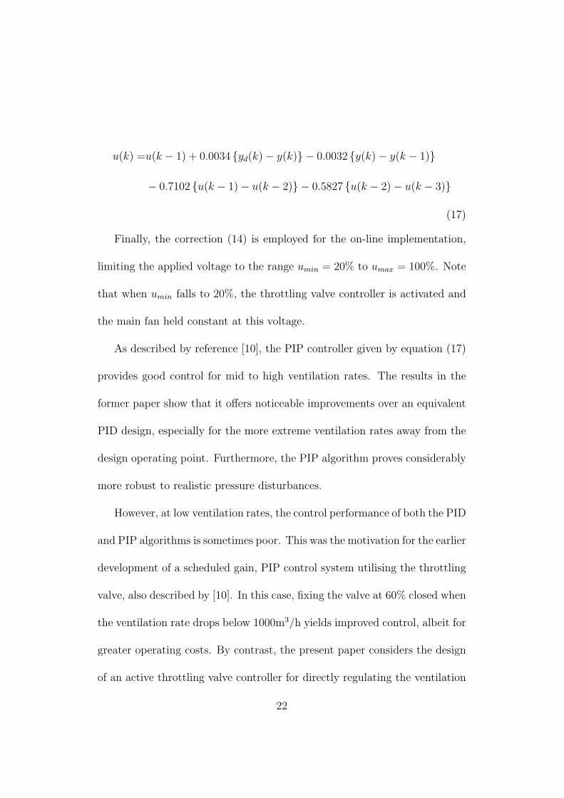
u(k) =u(k − 1) + 0.0034 {yd(k)− y(k)} − 0.0032 {y(k)− y(k − 1)}

− 0.7102 {u(k − 1)− u(k − 2)} − 0.5827 {u(k − 2)− u(k − 3)}

(17)

Finally, the correction (14) is employed for the on-line implementation,

limiting the applied voltage to the range umin = 20% to umax = 100%. Note

that when umin falls to 20%, the throttling valve controller is activated and

the main fan held constant at this voltage.

As described by reference [10], the PIP controller given by equation (17)

provides good control for mid to high ventilation rates. The results in the

former paper show that it offers noticeable improvements over an equivalent

PID design, especially for the more extreme ventilation rates away from the

design operating point. Furthermore, the PIP algorithm proves considerably

more robust to realistic pressure disturbances.

However, at low ventilation rates, the control performance of both the PID

and PIP algorithms is sometimes poor. This was the motivation for the earlier

development of a scheduled gain, PIP control system utilising the throttling

valve, also described by [10]. In this case, fixing the valve at 60% closed when

the ventilation rate drops below 1000m3/h yields improved control, albeit for

greater operating costs. By contrast, the present paper considers the design

of an active throttling valve controller for directly regulating the ventilation

22

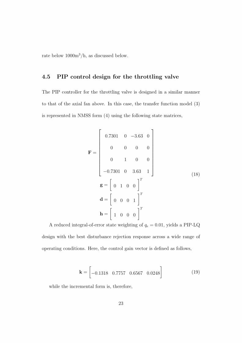
rate below 1000m3/h, as discussed below.

4.5 PIP control design for the throttling valve

The PIP controller for the throttling valve is designed in a similar manner

to that of the axial fan above. In this case, the transfer function model (3)

is represented in NMSS form (4) using the following state matrices,

F =

0.7301 0 −3.63 0

0 0 0 0

0 1 0 0

−0.7301 0 3.63 1

g =

[

0 1 0 0

]T

d =

[

0 0 0 1

]T

h =

[

1 0 0 0

]T

(18)

A reduced integral-of-error state weighting of qe = 0.01, yields a PIP-LQ

design with the best disturbance rejection response across a wide range of

operating conditions. Here, the control gain vector is defined as follows,

k =

[

−0.1318 0.7757 0.6567 0.0248

]

(19)

while the incremental form is, therefore,

23

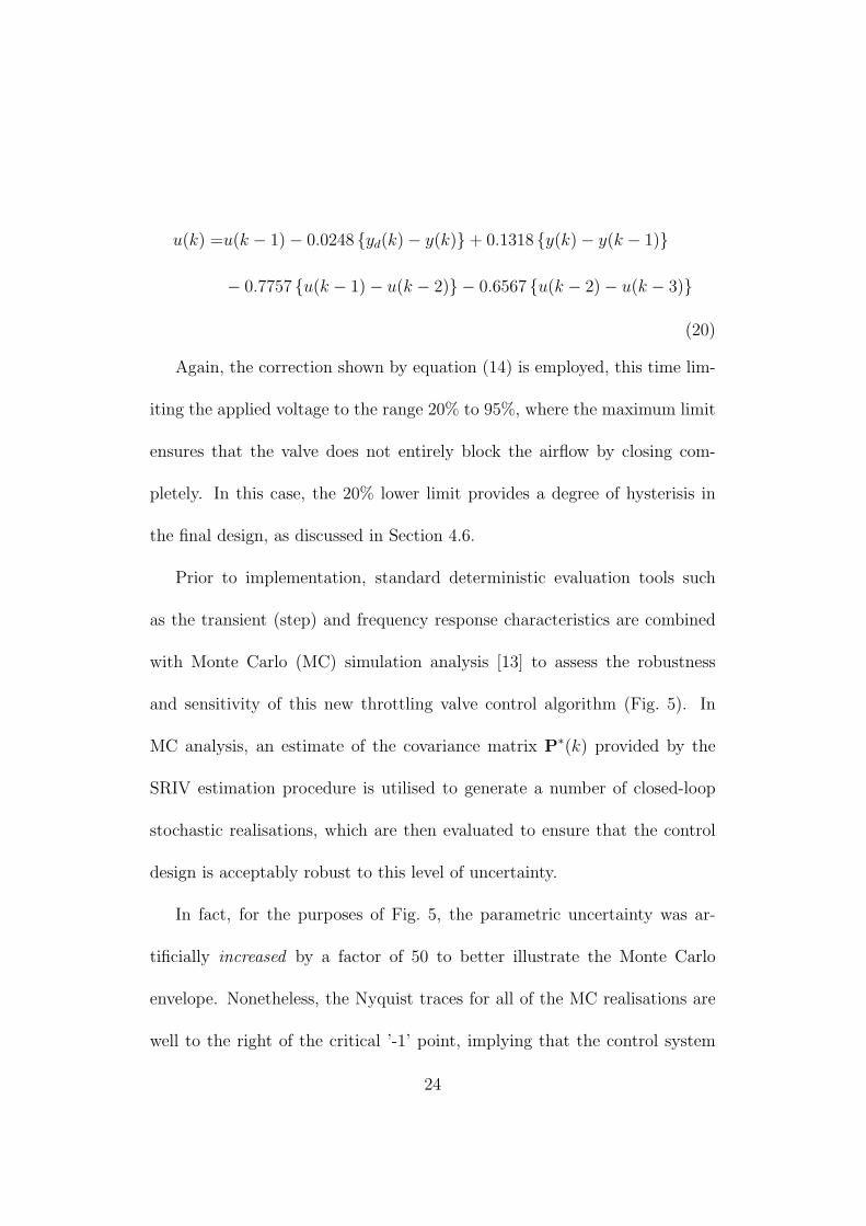
u(k) =u(k − 1)− 0.0248 {yd(k)− y(k)}+ 0.1318 {y(k)− y(k − 1)}

− 0.7757 {u(k − 1)− u(k − 2)} − 0.6567 {u(k − 2)− u(k − 3)}

(20)

Again, the correction shown by equation (14) is employed, this time lim-

iting the applied voltage to the range 20% to 95%, where the maximum limit

ensures that the valve does not entirely block the airflow by closing com-

pletely. In this case, the 20% lower limit provides a degree of hysterisis in

the final design, as discussed in Section 4.6.

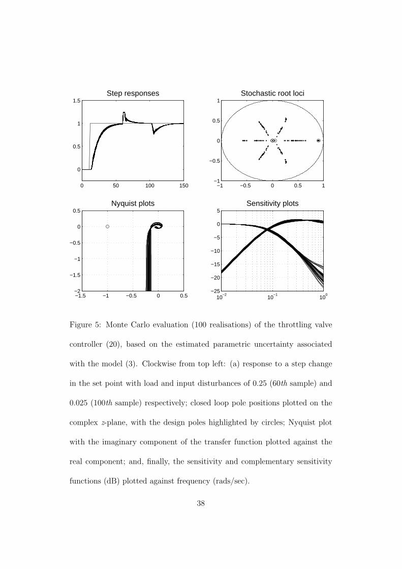
Prior to implementation, standard deterministic evaluation tools such

as the transient (step) and frequency response characteristics are combined

with Monte Carlo (MC) simulation analysis [13] to assess the robustness

and sensitivity of this new throttling valve control algorithm (Fig. 5). In

MC analysis, an estimate of the covariance matrix P∗(k) provided by the

SRIV estimation procedure is utilised to generate a number of closed-loop

stochastic realisations, which are then evaluated to ensure that the control

design is acceptably robust to this level of uncertainty.

In fact, for the purposes of Fig. 5, the parametric uncertainty was ar-

tificially increased by a factor of 50 to better illustrate the Monte Carlo

envelope. Nonetheless, the Nyquist traces for all of the MC realisations are

well to the right of the critical ’-1’ point, implying that the control system

24

yields highly stable responses despite the simulated parametric uncertainty.

Similarly, it is clear that all of the closed-loop pole positions (or stochastic

root loci) are well inside the unit circle on the complex z-plane. Finally, note

that although just 100 realisations are employed in the figure, the results

change insignificantly if more realisations (1000) are utilised.

4.6 Combined fan/valve controller

The new fan/valve PIP control system features simple rules to switch between

the two algorithms (17) and (20). For mid to high ventilation rates, the

throttling valve is held fully open to minimise operating costs. However,

for low ventilation rates or during particularly strong disturbances, control

switches to the throttling valve. In particular, the axial fan voltage is held

constant at 20% when the control input determined by (17) would otherwise

fall below this threshold. At this point, the throttling valve becomes the

control actuator using (20).

Similarly, when the applied voltage to the throttling valve falls to 20%,

the valve is immediately opened fully and the axial fan controller (17) reacti-

vated. This transition from throttling valve to fan control inherently includes

a degree of hysteresis, which stops undesirable switching between the two al-

gorithms when the ventilation rate is close to 1000m3/h. Finally, note that

25

both algorithms utilise specially developed initialisation settings to a ensure

smooth transition between them [18].

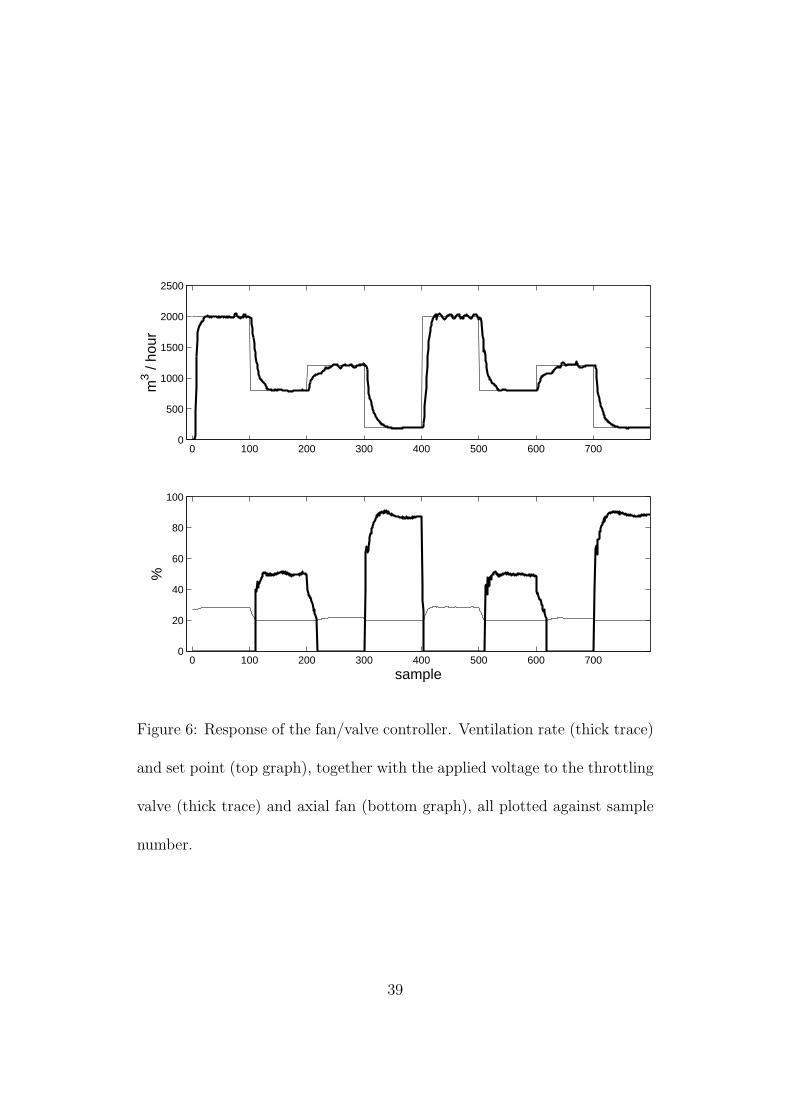
As illustrated by Fig. 6, the approach works extremely well in practice.

Here, the bottom graph shows the fluctuating control signals of both the fan

and the throttling valve, as the ventilation rate is successfully maintained at

a number of operating levels. Fig. 7 shows the equivalent power consumption

and applied voltage to the disturbance fan. Note that power consumption is

based on the axial fan voltage, since the throttling valve consumes compara-

tively little power for its operation. As discussed in Section 2, the disturbance

fan represents realistic pressure variations.

5 Control evaluation

The present section compares the performance and operating costs of the PIP

controller above, with an equivalent commercial design also implemented on

the Leuven ventilation chamber. Here, the commercial controller is based on

a PID algorithm combined with a number of ad hoc rules for adjustment of

the throttling valve.

For ventilation rates in the region of 3000m3/h, the PIP and commercial

designs behave in a similar fashion, although the latter appears to respond

slightly slower to changes in the set point. For the highest ventilation rates

26

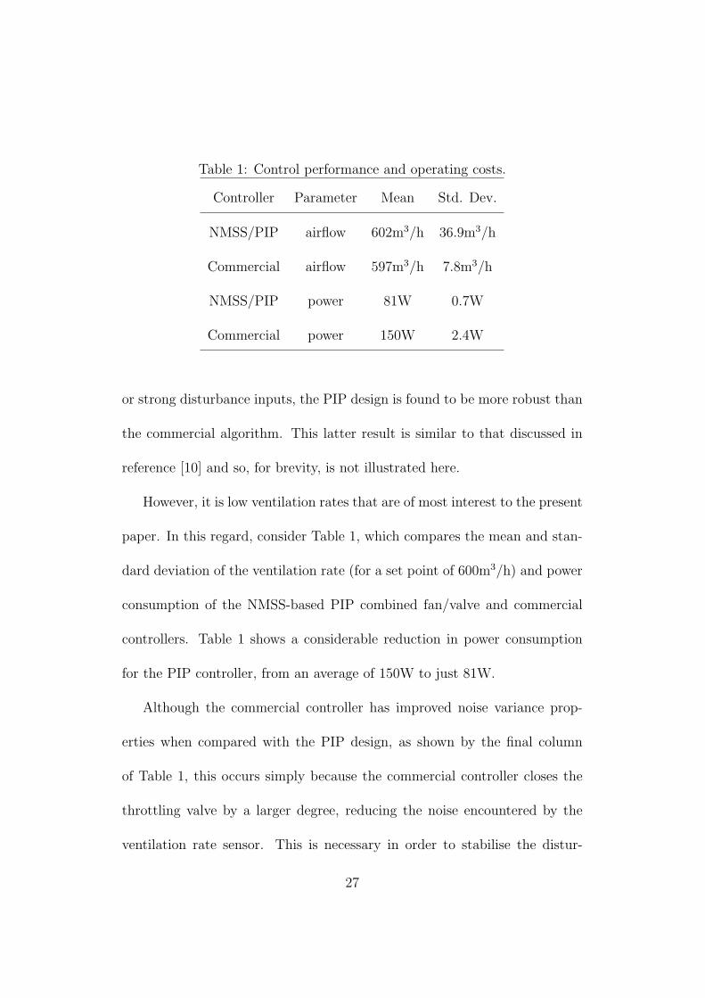
Table 1: Control performance and operating costs.

Controller Parameter Mean Std. Dev.

NMSS/PIP airflow 602m3/h 36.9m3/h

Commercial airflow 597m3/h 7.8m3/h

NMSS/PIP power 81W 0.7W

Commercial power 150W 2.4W

or strong disturbance inputs, the PIP design is found to be more robust than

the commercial algorithm. This latter result is similar to that discussed in

reference [10] and so, for brevity, is not illustrated here.

However, it is low ventilation rates that are of most interest to the present

paper. In this regard, consider Table 1, which compares the mean and stan-

dard deviation of the ventilation rate (for a set point of 600m3/h) and power

consumption of the NMSS-based PIP combined fan/valve and commercial

controllers. Table 1 shows a considerable reduction in power consumption

for the PIP controller, from an average of 150W to just 81W.

Although the commercial controller has improved noise variance prop-

erties when compared with the PIP design, as shown by the final column

of Table 1, this occurs simply because the commercial controller closes the

throttling valve by a larger degree, reducing the noise encountered by the

ventilation rate sensor. This is necessary in order to stabilise the distur-

27

bance response of the PID algorithm, but is not required in the PIP case.

This restricted airflow associated with the commercial controller inevitably

requires a higher applied voltage to the axial fan, resulting in the higher op-

erating cost. Furthermore, it should be pointed out that, in absolute terms,

the PIP controller performs very well indeed, as is clear from Fig. 6, well

within the performance requirements of a microclimate control system.

Finally, note that the previously developed, gain scheduled, PIP algo-

rithm [10], has similar power consumption characteristics to that of the com-

mercial controller. In this regard, the main advantage of the new combined

fan/valve PIP approach, is the reduced operating cost illustrated by Table 1.

For all the experiments discussed above, the disturbance fan operates

against the flow of air generated by the axial fan. However, by reinstalling

the disturbance fan in the reverse direction, it may be used to simulate

the effect of any natural ventilation present in the system. As discussed in

Section 2, such natural ventilation has the potential for further reducing the

power consumption of the axial fan.

The obvious advantage of the new fan/valve control configuration in this

context, is that the system automatically switches to throttling valve control

when the axial fan is not required. Preliminary results in this regard are

promising and offer the potential for further cost savings [18]. Current re-

search is concerned with evaluating the robustness and performance of such

28

an approach under a wide range of operating conditions, and this will be

reported in future publications.

6 Conclusion

This paper is concerned with Proportional-Integral-Plus (PIP) control of ven-

tilation rate in mechanically ventilated agricultural buildings. In particular,

the paper considers the design of a combined fan and throttling valve control

system for a 22m3 ventilation test chamber at the Katholieke Universiteit

Leuven, representing a section of a livestock building or glasshouse. In this

case, PIP controllers are developed for both the axial fan and a throttling

valve, where the latter is introduced to stabilise the airflow at low ventilation

rates.

For these experiments, separate PIP algorithms are designed and imple-

mented for both control actuators, using simple rules to switch between the

controllers as appropriate. This straightforward arrangement proves to work

very well in practice, as illustrated by Fig. 6. In particular, the fan/valve PIP

design yields significant reductions in power consumption when compared to

both a previously developed scheduled PIP design and a commercial con-

troller also optimised for the test chamber.

On the basis of the experiments discussed above, extrapolating the re-

29

duced operating cost of the new PIP ventilation controller to the total pro-

duction costs per housed animal, would yield significant savings. This clearly

makes the PIP algorithm a viable proposition, since the control implementa-

tion complexity is no greater than that of the PID-based commercial design

presently employed.

Acknowledgments

The authors are grateful for the support of the Engineering and Physical Sci-

ences Research Council (EPSRC). This publication is expanded and updated

from reference [19], first presented at the 16th International Conference on

Systems Engineering (ICSE).

References

[1] G. A. Carpenter. Ventilation of buildings for intensively houses livestock.

In J. L. Montieth and L. E. Mont, editors, Heat loss from animals and

man, pages 389–403. Butterworths, London, 1974.

[2] J. M. Randall. Ventilation system design. In J. A. Clark, editor, En-

vironmental aspects of housing for animal production, pages 351–369.

Butterworths, London, 1981.

30

[3] A. J. Hebner, C. R. Boon, and G. H. Peugh. Air patterns and tur-

bulence in an experimental livestock building. Journal of Agricultural

Engineering Research, 64:209–226, 1996.

[4] E. Vranken. Analysis and Optimisation of Ventilation Control in Live-

stock Buildings. PhD thesis, Katholieke Universiteit Leuven, Belgium,

1999.

[5] P. F. Davis and A. W. Hooper. Improvement of greenhouse heating

control. IEE Proceedings - Control Theory and Applications, 138:249,

1991.

[6] N. Sigrimis, K. G. Arvanitis, I. K. Kookos, and P. N. Paraskevopoulos.

H-infinity-pi controller tuning for greenhouse temperature control. In

IFAC 14th Triennial World Congress, Beijing, China, 1999.

[7] C. J. Taylor, P. C. Young, and A. Chotai. State space control system

design based on non-minimal state-variable feedback : Further generali-

sation and unification results. International Journal of Control, 73:1329–

1345, 2000.

[8] P. C. Young, M. A. Behzadi, C. L. Wang, and A. Chotai. Direct dig-

ital and adaptive control by input-output, state variable feedback pole

assignment. International Journal of Control, 46:1867–1881, 1987.

31

[9] L. Price, P. C. Young, D. Berckmans, K. Janssens, and C. J. Taylor.

Data-based mechanistic modelling (dbm) and control of mass and energy

transfer in agricultural buildings. Annual Reviews in Control, 23:71–83,

1999.

[10] C. J. Taylor, P. Leigh, L. Price, P. C. Young, D. Berckmans, K. Janssens,

E. Vranken, and R. Gevers. Proportional-integral-plus (pip) control of

ventilation rate in agricultural buildings. Control Engineering Practice,

12:225–233, 2004.

[11] A. P. Robertson and A. G. Glass. The silsoe structures building - its

design, instrumentation and research facilities. Divisional note, AFRC

Institute of Engineering Research, Wrest Park, Silsoe, Bedford, UK,

1988.

[12] P. C. Young. Recursive Estimation and Time Series Analysis. Springer-

Verlag, Berlin, 1984.

[13] P. C. Young. Simplified refined instrumental variable (sriv) estimation

and true digital control (tdc): a tutorial introduction. In 1st European

Control Conference, pages 1295–1306, Grenoble, 1991.

[14] P. C. Young and A. J. Jakeman. Refined instrumental variable meth-

32

ods of recursive time-series analysis, part 3: extensions. International

Journal of Control, 31:741–764, 1980.

[15] P. C. Young, M. Lees, A. Chotai, W. Tych, and Z. S. Chalabi. Mod-

elling and pip control of a glasshouse micro-climate. Control Engineering

Practice, 2(4):591–604, 1994.

[16] K. J. Astrom and B. Wittenmark. Computer controlled systems: theory

and design. Information and system sciences series. Prentice-Hall, 1984.

[17] A. Chotai, P. C. Young, P. McKenna, and W. Tych. Pip design for

delta-operator systems: Part 2, mimo systems. International Journal of

Control, 70:149–168, 1998.

[18] P. A. Leigh. Modelling and Control of Micro-Environmental Systems.

PhD thesis, Institute of Environmental and Natural Sciences, Lancaster

University, UK, 2002.

[19] P. Leigh, C. J. Taylor, A. Chotai, P. C. Young, and E. Vranken. Imple-

mentation of a combined fan and valve control design in a ventilation

chamber. In K. J. Burnham and O. C. L. Haas, editors, 16th Inter-

national Conference on Systems Engineering, pages 423–428, Coventry

University, UK, September 2003.

33

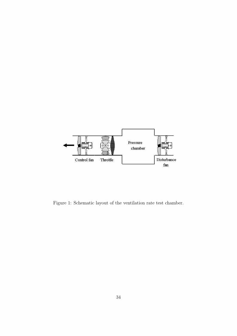
Figure 1: Schematic layout of the ventilation rate test chamber.

34

0 10 20 30 40 50 60 70 80 90 100

0

1000

2000

3000

4000

5000

6000

%

m3 /

h

valve 0%

valve 60%

dist 40%

fan 20%

Figure 2: Steady state power curves. Thin traces: airflow rate plotted

against control fan applied voltage for two different throttling valve settings,

fully open (circles) and 60% closed (triangles). Thick traces: airflow plotted

against throttling valve applied voltage, for control fan 20% (solid trace) and

disturbance fan 40% (dashed).

35

10 20 30 40 50 60 70 80 90 100 110600

650

700

750

800

m3 /

h

10 20 30 40 50 60 70 80 90 100 11045

50

55

60

65

sample

%

Figure 3: Open loop throttling valve experiment. Ventilation rate (dots; top

graph) and response of the identified model (3), together with the applied

voltage to the throttling valve (bottom graph), all plotted against sample

number.

36

yd(k) y(k)u(k)+/−+/−+/−

kI1− z−1

1

G(z−1)

B(z−1)

A(z−1)

F1(z−1)

f0

Figure 4: PIP control implemented in feedback form.

37

−1 −0.5 0 0.5 1−1

−0.5

0

0.5

1Stochastic root loci

−1.5 −1 −0.5 0 0.5−2

−1.5

−1

−0.5

0

0.5Nyquist plots

10−2

10−1

100

−25

−20

−15

−10

−5

0

5Sensitivity plots

0 50 100 150

0

0.5

1

1.5Step responses

Figure 5: Monte Carlo evaluation (100 realisations) of the throttling valve

controller (20), based on the estimated parametric uncertainty associated

with the model (3). Clockwise from top left: (a) response to a step change

in the set point with load and input disturbances of 0.25 (60th sample) and

0.025 (100th sample) respectively; closed loop pole positions plotted on the

complex z-plane, with the design poles highlighted by circles; Nyquist plot

with the imaginary component of the transfer function plotted against the

real component; and, finally, the sensitivity and complementary sensitivity

functions (dB) plotted against frequency (rads/sec).

38

0 100 200 300 400 500 600 7000

500

1000

1500

2000

2500

m3 /

hour

0 100 200 300 400 500 600 7000

20

40

60

80

100

sample

%

Figure 6: Response of the fan/valve controller. Ventilation rate (thick trace)

and set point (top graph), together with the applied voltage to the throttling

valve (thick trace) and axial fan (bottom graph), all plotted against sample

number.

39

0 100 200 300 400 500 600 7000

50

100

150

200

W

0 100 200 300 400 500 600 7000

10

20

30

40

50

sample

%

Figure 7: Power consumption (top graph) and applied voltage to the distur-

bance fan (bottom graph) for the response in Fig. 6.

40