Coupled simulation work˜ow - dynardo.de

Coupled simulation work�ow for the design of optimized

power electronic systems

Andreas Rosskopf pres

ente

d at

the

14th

Wei

mar

Opt

imiz

atio

n an

d St

ocha

stic

Day

s 20

17

Sour

ce:

ww

w.d

ynar

do.d

e/en

/libr

ary

Seite 2 von 21, WOST 2017 A. Rosskopf, 01./02. Juni 2017 © Fraunhofer IISB

AGENDA

1. Initial situation

2. Design workflow for power electronic systems

3. Parameter variation

4. Practical applicability of the MoP

5. Genetic optimization

6. Conclusion


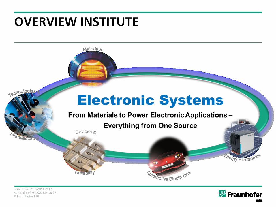
OVERVIEW INSTITUTE


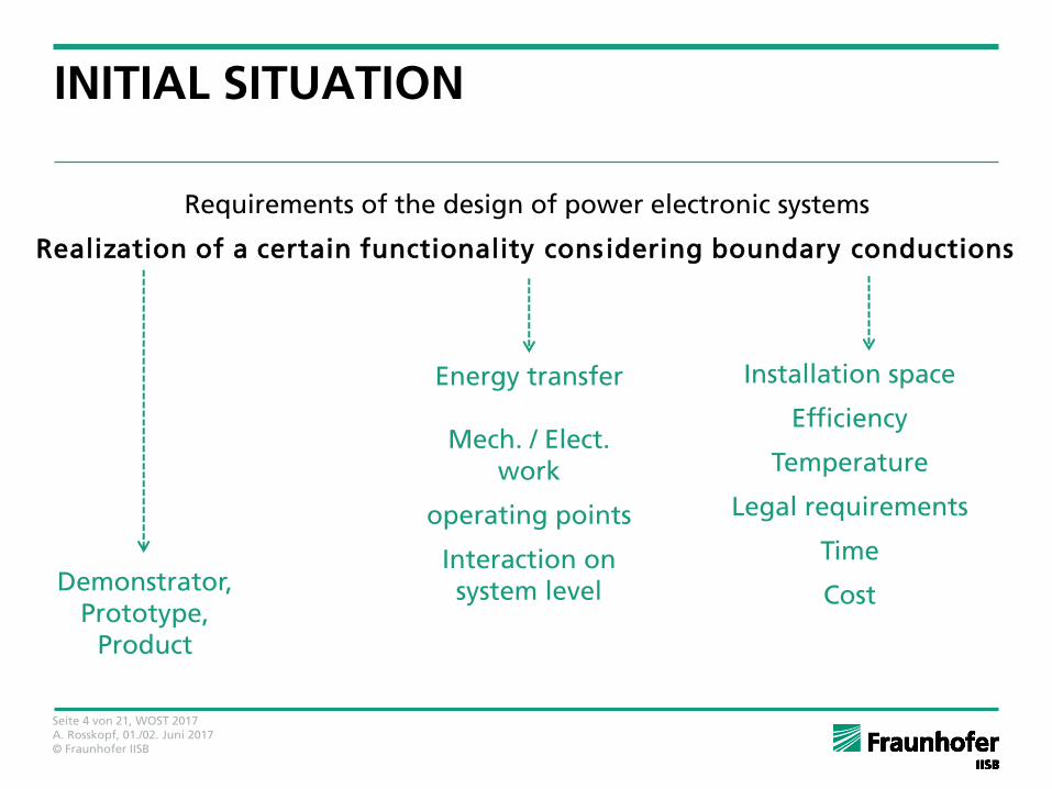
INITIAL SITUATION

Energy transfer

Mech. / Elect. work

operating points

Interaction on system level

Installation space

Efficiency

Temperature

Legal requirements

Time

Cost

Requirements of the design of power electronic systems

Realization of a certain functionality considering boundary conductions

Demonstrator, Prototype,

Product


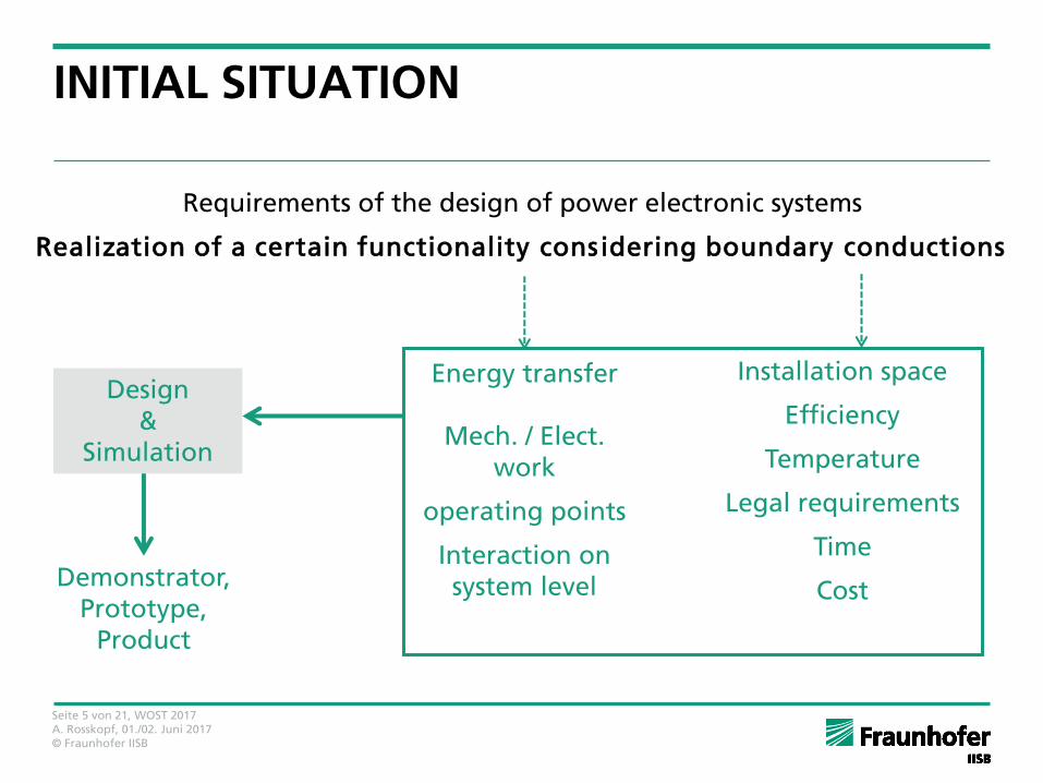
INITIAL SITUATION

Energy transfer

Mech. / Elect. work

operating points

Interaction on system level

Requirements of the design of power electronic systems

Realization of a certain functionality considering boundary conductions

Demonstrator, Prototype,

Product

Design &

Simulation

Installation space

Efficiency

Temperature

Legal requirements

Time

Cost


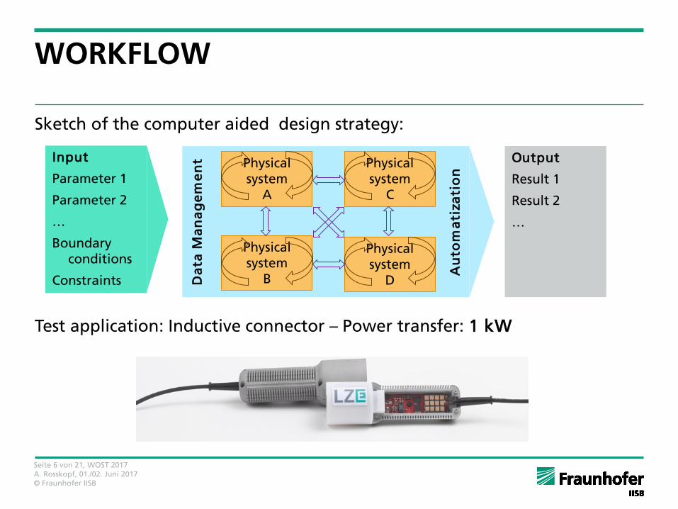
Da

ta M

an

ag

em

en

t

Au

tom

ati

za

tio

n Physical

system A

Physical system

B

Physical system

C

Physical system

D

Input

Parameter 1

Parameter 2

…

Boundary conditions

Constraints

Output

Result 1

Result 2

…

Sketch of the computer aided design strategy:

Test application: Inductive connector – Power transfer: 1 kW

WORKFLOW


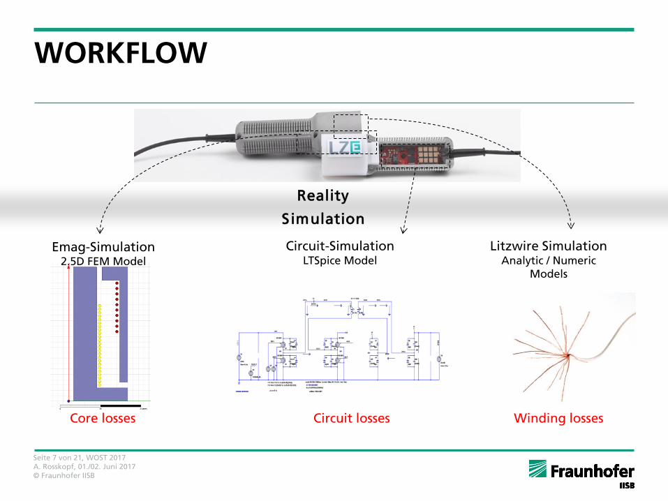
WORKFLOW

Reality

Simulation

Emag-Simulation 2.5D FEM Model

Circuit-Simulation LTSpice Model

Litzwire Simulation Analytic / Numeric

Models

Core losses Circuit losses Winding losses


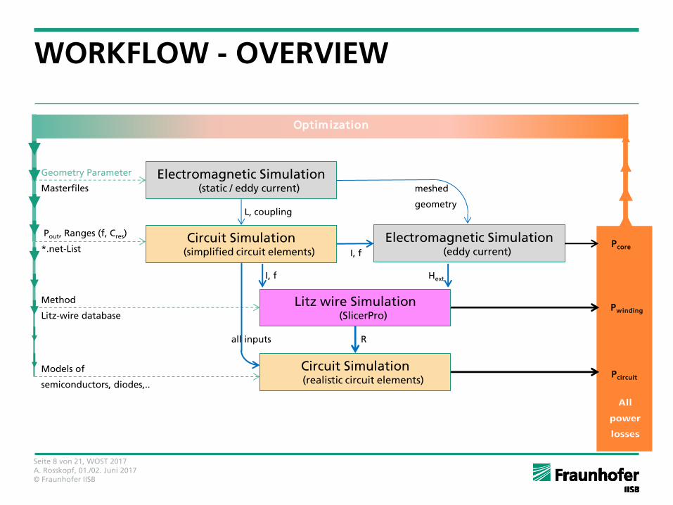
WORKFLOW - OVERVIEW

Electromagnetic Simulation (static / eddy current)

Circuit Simulation (simplified circuit elements)

Litz wire Simulation (SlicerPro)

Geometry Parameter

Masterfiles

L, coupling

I, f

Pout, Ranges (f, Cres)

*.net-List

Method

Litz-wire database

Electromagnetic Simulation (eddy current) I, f

meshed

geometry

Hext

Circuit Simulation (realistic circuit elements)

R

Models of

semiconductors, diodes,..

Pcore

Pwinding

Pcircuit

Optimization

all inputs


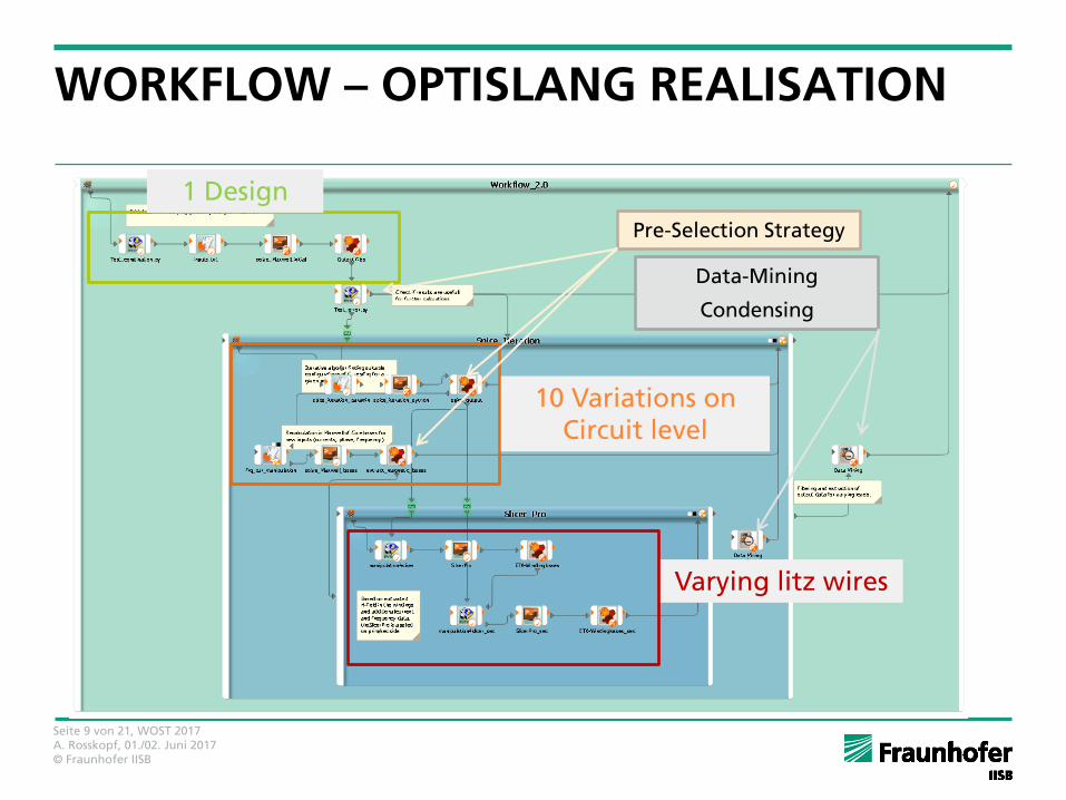
WORKFLOW – OPTISLANG REALISATION

1 Design

10 Variations on Circuit level

Varying litz wires

Pre-Selection Strategy

Data-Mining

Condensing


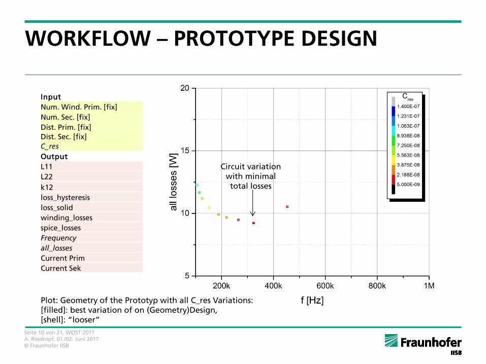
WORKFLOW – PROTOTYPE DESIGN

Input

Num. Wind. Prim. [fix]

Num. Sec. [fix]

Dist. Prim. [fix]

Dist. Sec. [fix]

C_res

Output

L11

L22

k12

loss_hysteresis

loss_solid

winding_losses

spice_losses

Frequency

all_losses

Current Prim

Current Sek

Plot: Geometry of the Prototyp with all C_res Variations: [filled]: best variation of on (Geometry)Design, [shell]: “looser”

Circuit variation with minimal total losses


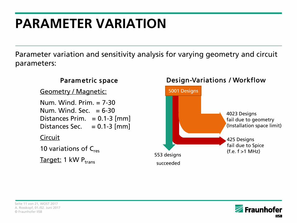
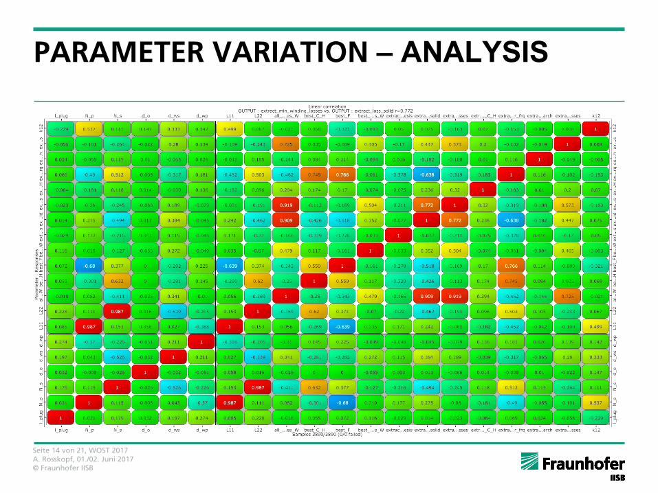
Parameter variation and sensitivity analysis for varying geometry and circuit parameters:

PARAMETER VARIATION

Parametric space

Geometry / Magnetic:

Num. Wind. Prim. = 7-30 Num. Wind. Sec. = 6-30 Distances Prim. = 0.1-3 [mm] Distances Sec. = 0.1-3 [mm]

Circuit

10 variations of Cres

Target: 1 kW Ptrans

Design-Variations / Workflow

4023 Designs fail due to geometry (Installation space limit)

425 Designs fail due to Spice (f.e. f >1 MHz)

553 designs

succeeded


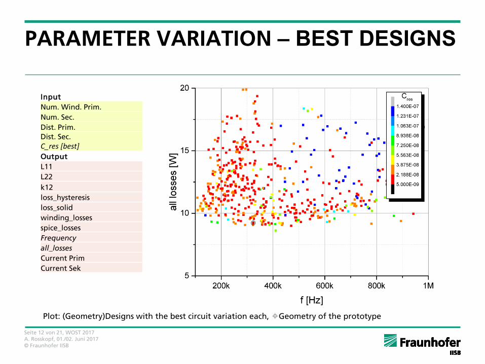
PARAMETER VARIATION – BEST DESIGNS

Plot: (Geometry)Designs with the best circuit variation each, Geometry of the prototype

Input

Num. Wind. Prim.

Num. Sec.

Dist. Prim.

Dist. Sec.

C_res [best]

Output

L11

L22

k12

loss_hysteresis

loss_solid

winding_losses

spice_losses

Frequency

all_losses

Current Prim

Current Sek


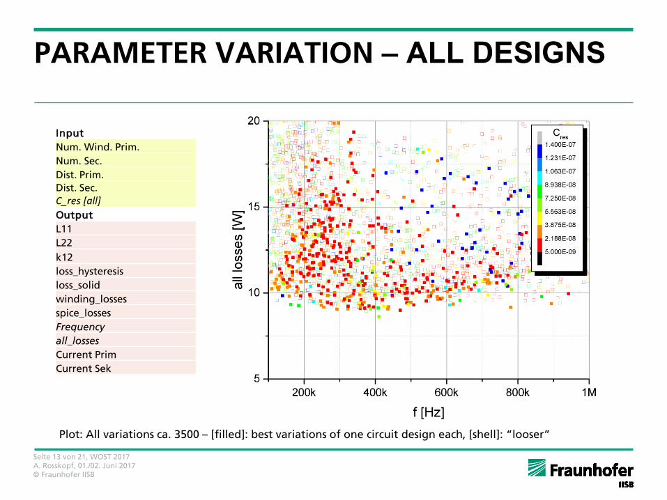
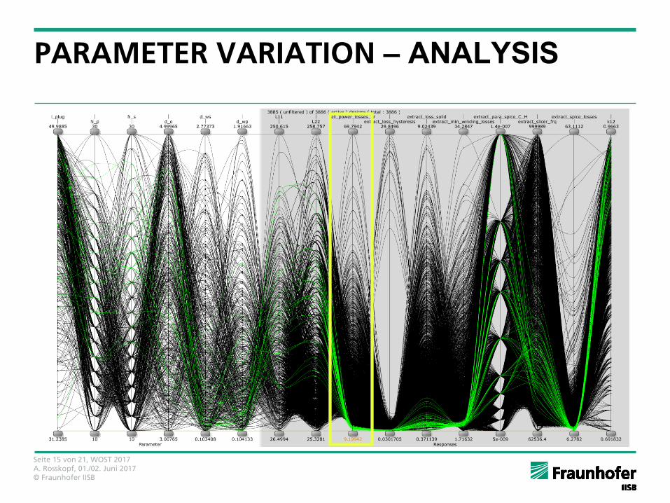
PARAMETER VARIATION – ALL DESIGNS

Plot: All variations ca. 3500 – [filled]: best variations of one circuit design each, [shell]: “looser”

Input

Num. Wind. Prim.

Num. Sec.

Dist. Prim.

Dist. Sec.

C_res [all]

Output

L11

L22

k12

loss_hysteresis

loss_solid

winding_losses

spice_losses

Frequency

all_losses

Current Prim

Current Sek


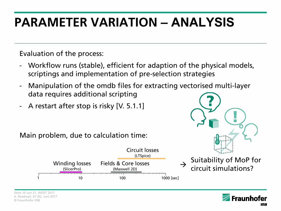
PARAMETER VARIATION – ANALYSIS





1 10 100 1000 [sec]

Fields & Core losses (Maxwell 2D)

Winding losses (SlicerPro)

Circuit losses (LTSpice)

Evaluation of the process:

- Workflow runs (stable), efficient for adaption of the physical models, scriptings and implementation of pre-selection strategies

- Manipulation of the omdb files for extracting vectorised multi-layer data requires additional scripting

- A restart after stop is risky [V. 5.1.1]

Suitability of MoP for circuit simulations?

Main problem, due to calculation time:


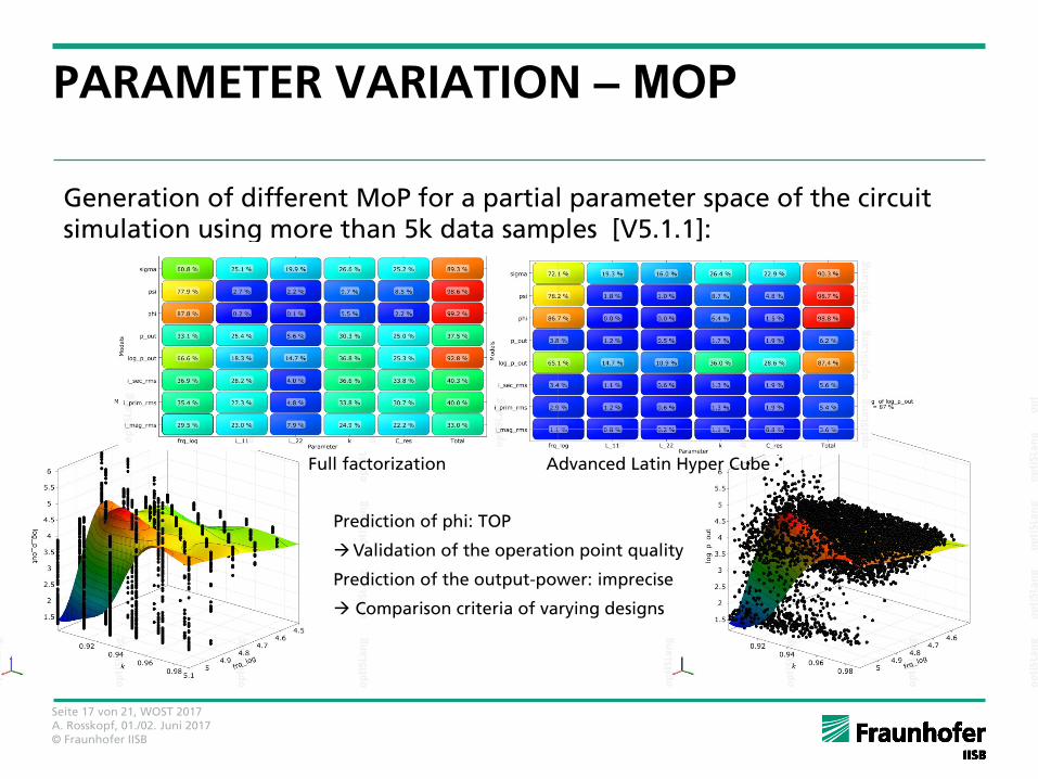
PARAMETER VARIATION – MOP

Generation of different MoP for a partial parameter space of the circuit simulation using more than 5k data samples [V5.1.1]:

Full factorization Advanced Latin Hyper Cube

Prediction of phi: TOP

Validation of the operation point quality

Prediction of the output-power: imprecise

Comparison criteria of varying designs


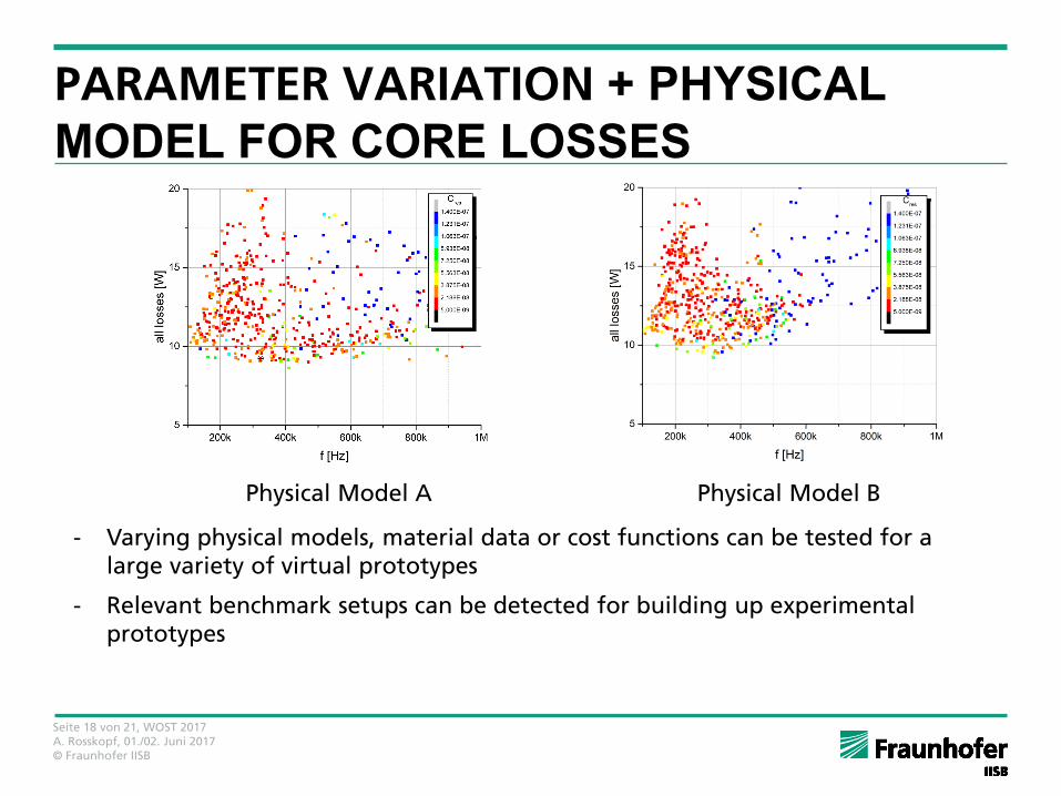
PARAMETER VARIATION + PHYSICAL

MODEL FOR CORE LOSSES

Physical Model A Physical Model B

- Varying physical models, material data or cost functions can be tested for a large variety of virtual prototypes

- Relevant benchmark setups can be detected for building up experimental prototypes


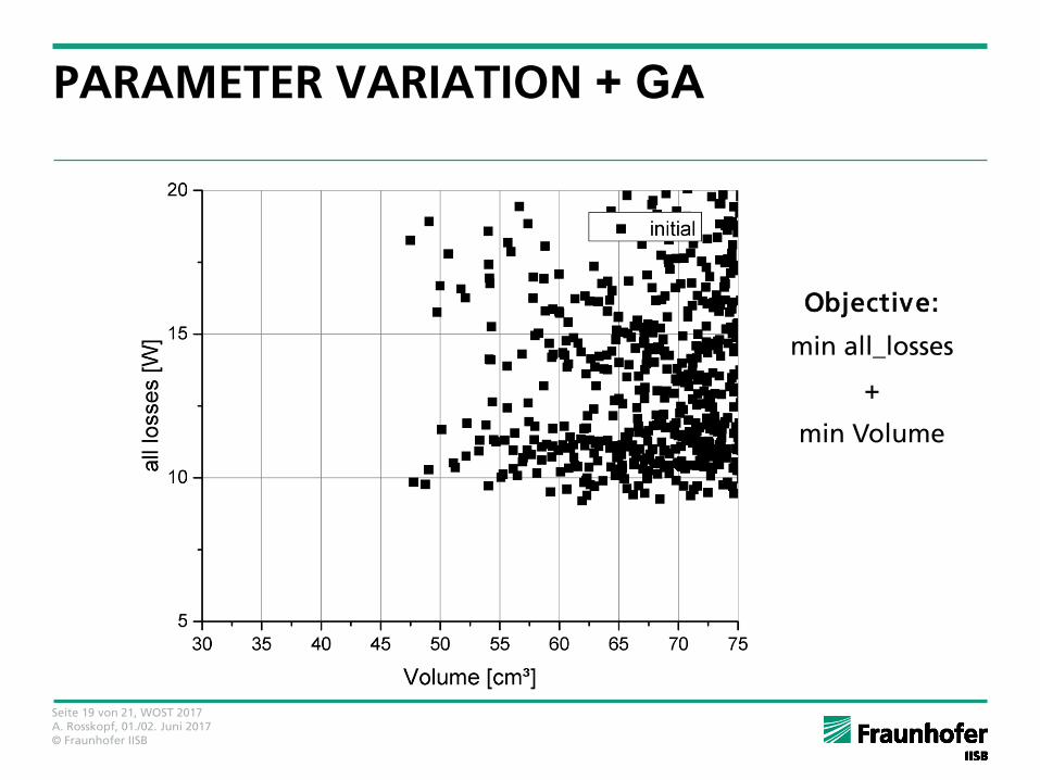
PARAMETER VARIATION + GA

Objective:

min all_losses

+

min Volume


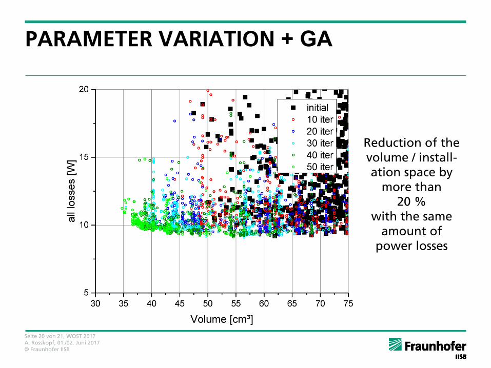
PARAMETER VARIATION + GA

Reduction of the volume / install-ation space by

more than 20 %

with the same amount of

power losses


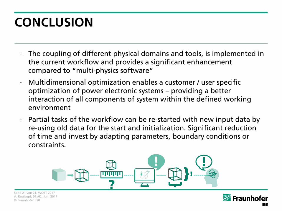
CONCLUSION

- The coupling of different physical domains and tools, is implemented in the current workflow and provides a significant enhancement compared to “multi-physics software”

- Multidimensional optimization enables a customer / user specific optimization of power electronic systems – providing a better interaction of all components of system within the defined working environment

- Partial tasks of the workflow can be re-started with new input data by re-using old data for the start and initialization. Significant reduction of time and invest by adapting parameters, boundary conditions or constraints.

Documents

Coupled simulation work˜ow - dynardo.de