Course pack unit 5

Course: MCASubject: Computer Oriented Numerical

Statistical MethodsUnit-5

RAI UNIVERSITY, AHMEDABAD

\

RAI UNIVERSITY, AHMEDABAD 1

Unit-V-Regression

Sr.

No.

Name of the Topic Page

No.

1 Introduction and Definition of Regression Analysis 2

2 Regression lines ,Properties and its explanation 3

3 Regression coefficients and its Properties 5

4 Difference between Regression and Correlation 6

5 Example based on the Regression line and Regression Co-

efficients

7

6 Example based on the fitting of regression line and estimation for

bivariate frequency distribution

13

7 Advantage and limitations of Regression Analysis 17

8 References 18

9 Exercise 19


Unit-V-Regression

1.1 Introduction:

If two variables are significantly correlated, and if there is some theoretical basis

for doing so, it is possible to predict (estimate) values of one variable from the

other. This observation leads to a very important concept known as ‘Regression

Analysis’.

For example, if we know that the advertising and sales are correlated we find out

expected amount of sales for a given advertising expenditure for attaining a given

amount of sales. Similarly if we know the yield of rice and rainfall are closely

related we may find out the amount of rain is required to achieve a certain

production figure.

In general Regression analysis means the estimation or prediction of the unknown

value of one variable from the known value of the other variable. It is one of the

most important statistical tools which is extensively used in almost all sciences –

Natural, Social and Physical.

1.2 Definition:

The dictionary meaning of ‘Regression’ is returning or going back. The term

‘Regression’ is first used by Sir Francis Galton (1822-1911) in 1877 while

studying the relationship between the height of father and sons. This term was

introduced by him in the paper of “Regression towards Mediocrity in healthcare

structure”.

Regression analysis was explained by M. M. Blair as follows:

“Regression analysis is a mathematical measure of the average relationship

between two or more variables in terms of the original units of the data”.


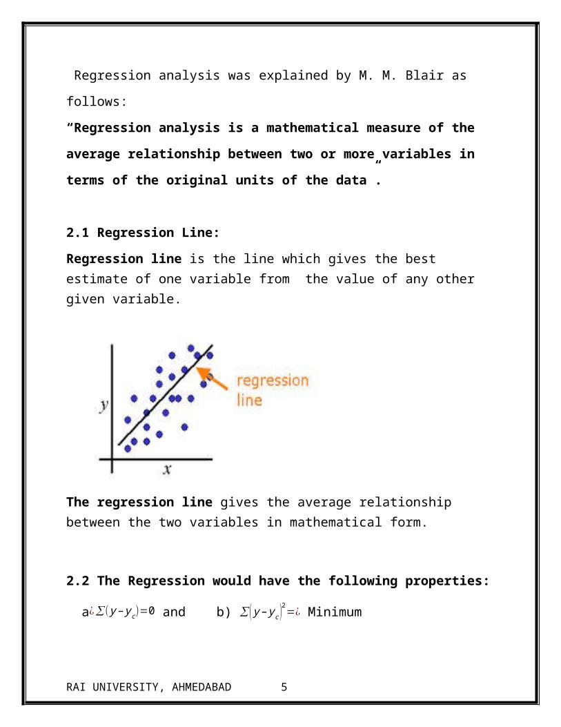
2.1 Regression Line:

Regression line is the line which gives the best estimate of one variable from the value of any other given variable.

The regression line gives the average relationship between the two variables in mathematical form.

2.2 The Regression would have the following properties:

a¿∑( y – yc)=0 and b) ∑ ( y – yc)2=¿ Minimum

• For two variables X and Y, there are always two lines of regression –(A)Regression line of x on y :

It gives the best estimate for the value of X for any specific given values of Y

x=a+b y

where a = x- intercept

b = Slope of the line

x = Dependent variable

y = Independent variable

(B) Regression line of Y on :


• It gives the best estimate for the value of Y for any specific given values of X

y=a+bx

Where a= y - intercept

b = Slope of the line

y = Dependent variable

x= Independent variable

2.3 The Explanation of Regression Line

• In case of perfect correlation (positive or negative ) the two line of regression coincide.

• If the two R. line are far from each other then degree of correlation is less, & vice versa.

• The mean values of x & y can be obtained as the point of intersection of the two regression line.

• The higher degree of correlation between the variables, the angle between the lines is smaller & vice versa.

2.4 Regression Equation / Line & Method of Least Squares

2.4.1 Regression Equation of y on x

y=a+bx

• In order to obtain the values of ‘ a’ & ‘b ’

∑ y=na+b∑ x

∑xy=a∑ x+b∑ x2

2.4.2 Regression Equation of x on

x=c+dy

• In order to obtain the values of ‘ c ’ & ‘ d ’


∑x=nc+d ∑ y

∑xy=c∑ y+d∑ y2

3.1 Regression Coefficients:

The regression coefficient between two variables is a numerical measure showing the change in the value of one variable for a unit change in the value of the other variable.

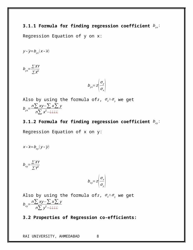
3.1.1 Formula for finding regression coefficient b yx :

Regression Equation of y on x:

y – y=byx(x – x )

b yx=∑XY

∑ X2

b yx=r ( σ yσ x )Also by using the formula ofr, σ x∧σ y we get b yx=

n∑ xy−∑ x∑ y

n∑ x2−¿¿¿¿

3.1.2 Formula for finding regression coefficient bxy :

Regression Equation of x on y:

x – x=bxy( y – y)

bxy=∑XY

∑Y 2

bxy=r ( σ xσ y )Also by using the formula ofr, σ x∧σ y we get bxy=

n∑ xy−∑ x∑ y

n∑ y2−¿¿¿¿

3.2 Properties of Regression co-efficients:


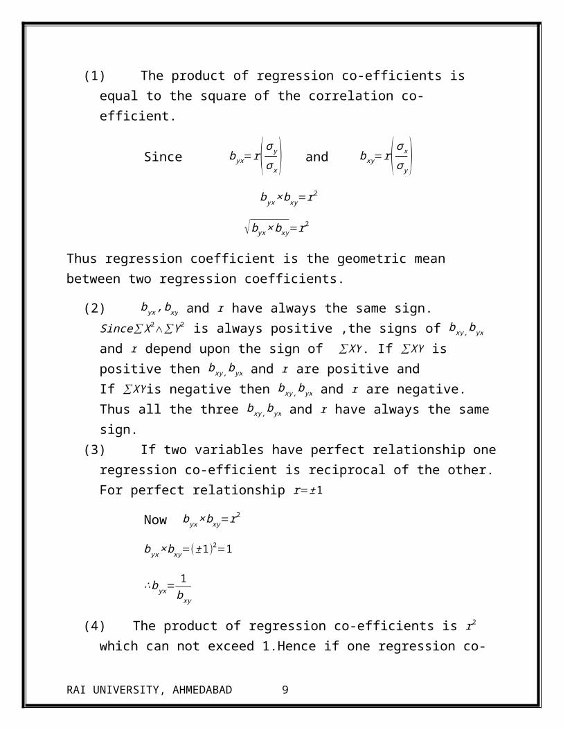
(1) The product of regression co-efficients is equal to the square of the correlation co-efficient.

Since b yx=r ( σ yσ x ) and bxy=r ( σ xσ y ) b yx×bxy=r

2

√b yx×bxy=r2

Thus regression coefficient is the geometric mean between two regression coefficients.

(2) b yx ,bxy and r have always the same sign.Since∑ X2∧∑Y 2 is always positive ,the signs of bxy ,b yx and r depend upon the sign of ∑XY . If ∑XY is positive then bxy ,b yx and r are positive andIf ∑XY is negative then bxy ,b yx and r are negative. Thus all the three bxy ,b yx and r have always the same sign.

(3) If two variables have perfect relationship one regression co-efficient is reciprocal of the other.For perfect relationship r=±1

Now b yx×bxy=r2

b yx×bxy=(±1)2=1

∴b yx=1bxy

(4)The product of regression co-efficients is r2 which can not exceed 1.Hence if one regression co-efficient is greater than 1, the other regression co-efficient is must be less than 1.

(5) The regression co-efficients are independent of change of origin but not of scale.

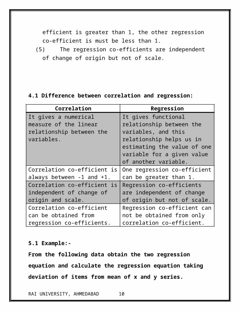
4.1 Difference between correlation and regression:


Correlation RegressionIt gives a numerical measure of the linear relationship between the variables.

It gives functional relationship between the variables, and this relationship helps us in estimating the value of one variable for a given value of another variable.

Correlation co-efficient is always between -1 and +1.

One regression co-efficient can be greater than 1.

Correlation co-efficient is independent of change of origin and scale.

Regression co-efficients are independent of change of origin but not of scale.

Correlation co-efficient can be obtained from regression co-efficients.

Regression co-efficient can not be obtained from only correlation co-efficient.

5.1 Example:-

From the following data obtain the two regression equation and calculate the

regression equation taking deviation of items from mean of x and y series.

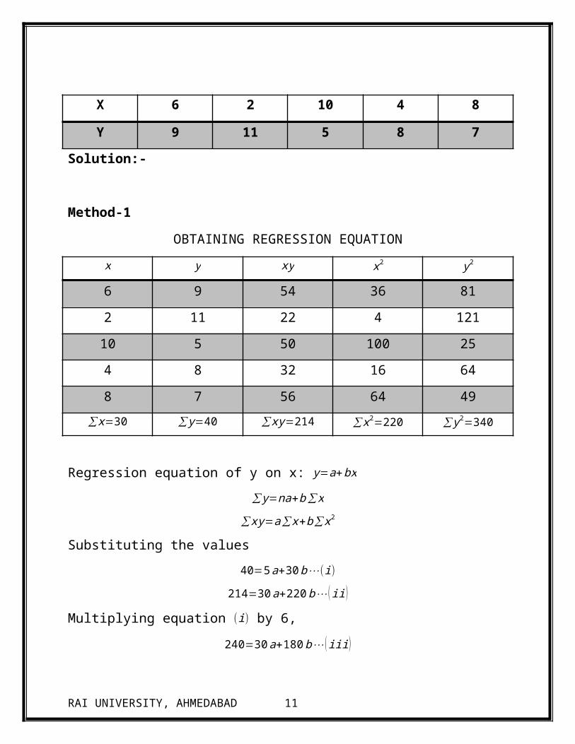
X 6 2 10 4 8

Y 9 11 5 8 7

Solution:-

Method-1

OBTAINING REGRESSION EQUATION

x y xy x2 y2

6 9 54 36 81

2 11 22 4 121

10 5 50 100 25

4 8 32 16 64

8 7 56 64 49


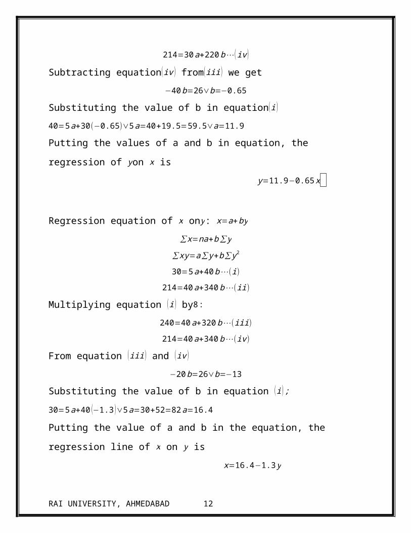
∑x=30 ∑ y=40 ∑xy=214 ∑x2=220 ∑ y2=340

Regression equation of y on x: y=a+bx

∑ y=na+b∑ x

∑ xy=a∑ x+b∑ x2

Substituting the values

40=5a+30b⋯ (i)

214=30a+220b⋯ ( ii )

Multiplying equation (i) by 6,

240=30a+180b⋯ ( iii)

214=30a+220b⋯ (iv )

Subtracting equation( iv ) from(iii ) we get

−40b=26∨b=−0.65

Substituting the value of b in equation( i )

40=5a+30 (−0.65)∨5a=40+19.5=59.5∨a=11.9

Putting the values of a and b in equation, the regression of yon x is

y=11.9−0.65x

Regression equation of x ony: x=a+by

∑ x=na+b∑ y

∑ xy=a∑ y+b∑ y2

30=5a+40b⋯ (i)

214=40a+340b⋯(ii)

Multiplying equation (i ) by8 :

240=40a+320b⋯ (iii)

214=40a+340b⋯(iv)

From equation ( iii ) and ( iv )

−20b=26∨b=−13

Substituting the value of b in equation ( i );


30=5a+40 (−1.3 )∨5a=30+52=82a=16.4

Putting the value of a and b in the equation, the regression line of x on y is

x=16.4−1.3 y

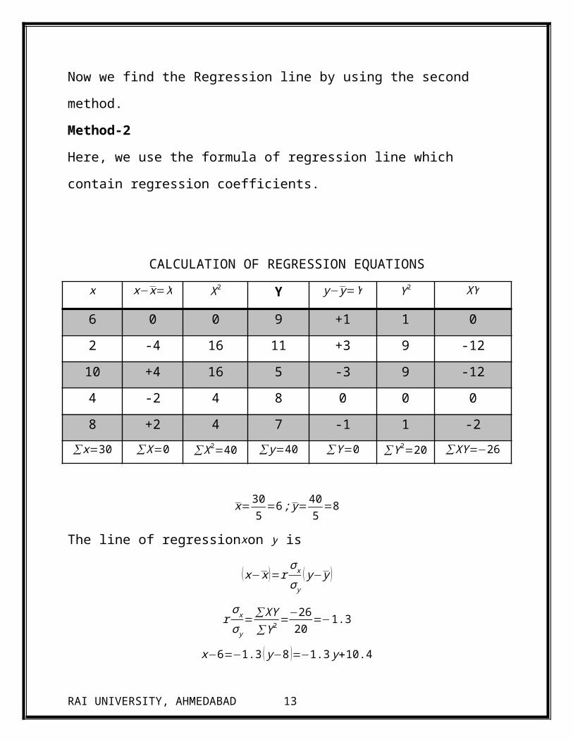
Now we find the Regression line by using the second method.

Method-2

Here, we use the formula of regression line which contain regression coefficients.

CALCULATION OF REGRESSION EQUATIONS

x x−x=X X2 Y y− y=Y Y 2 XY

6 0 0 9 +1 1 0

2 -4 16 11 +3 9 -12

10 +4 16 5 -3 9 -12

4 -2 4 8 0 0 0

8 +2 4 7 -1 1 -2

∑x=30 ∑X=0 ∑X 2=40 ∑ y=40 ∑Y=0 ∑Y 2=20 ∑XY=−26

x=305

=6 ; y=405

=8

The line of regressionxon y is

( x−x )=rσ xσ y

( y− y )

rσ xσ y

=∑XY∑Y 2 =−26

20=−1.3

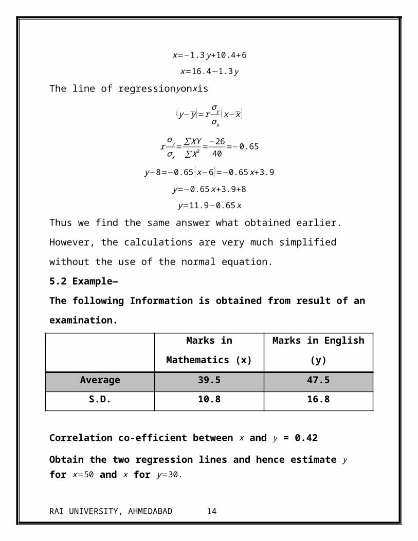
x−6=−1.3 ( y−8 )=−1.3 y+10.4

x=−1.3 y+10.4+6

x=16.4−1.3 y

The line of regressionyonxis


( y− y )=rσ yσ x

( x−x )

rσ yσ x

=∑XY∑X 2 =−26

40=−0.65

y−8=−0.65 ( x−6 )=−0.65 x+3.9

y=−0.65x+3.9+8

y=11.9−0.65x

Thus we find the same answer what obtained earlier. However, the calculations are

very much simplified without the use of the normal equation.

5.2 Example—

The following Information is obtained from result of an examination.

Marks in Mathematics

(x)

Marks in English (y)

Average 39.5 47.5

S.D. 10.8 16.8

Correlation co-efficient between x and y = 0.42

Obtain the two regression lines and hence estimate y for x=50 and x for y=30.

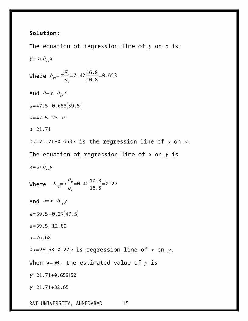
Solution:

The equation of regression line of y on x is:

y=a+b yx x

Where b yx=rσ yσ x

=0.4216.810.8

=0.653

And a= y−byx x

a=47.5−0.653 (39.5 )

a=47.5−25.79

a=21.71


∴ y=21.71+0.653 x is the regression line of y on x .

The equation of regression line of x on y is

x=a+bxy y

Where bxy=rσxσ y

=0.4210.816.8

=0.27

And a=x−bxy y

a=39.5−0.27 (47.5 )

a=39.5−12.82

a=26.68

∴ x=26.68+0.27 y is regression line of x on y.

When x=50 , the estimated value of y is

y=21.71+0.653 (50 )

y=21.71+32.65

y=54.36

When y=30 , the estimated value of x is

x=26.68+0.27 (30 )

x=26.68+8.10

x=34.78

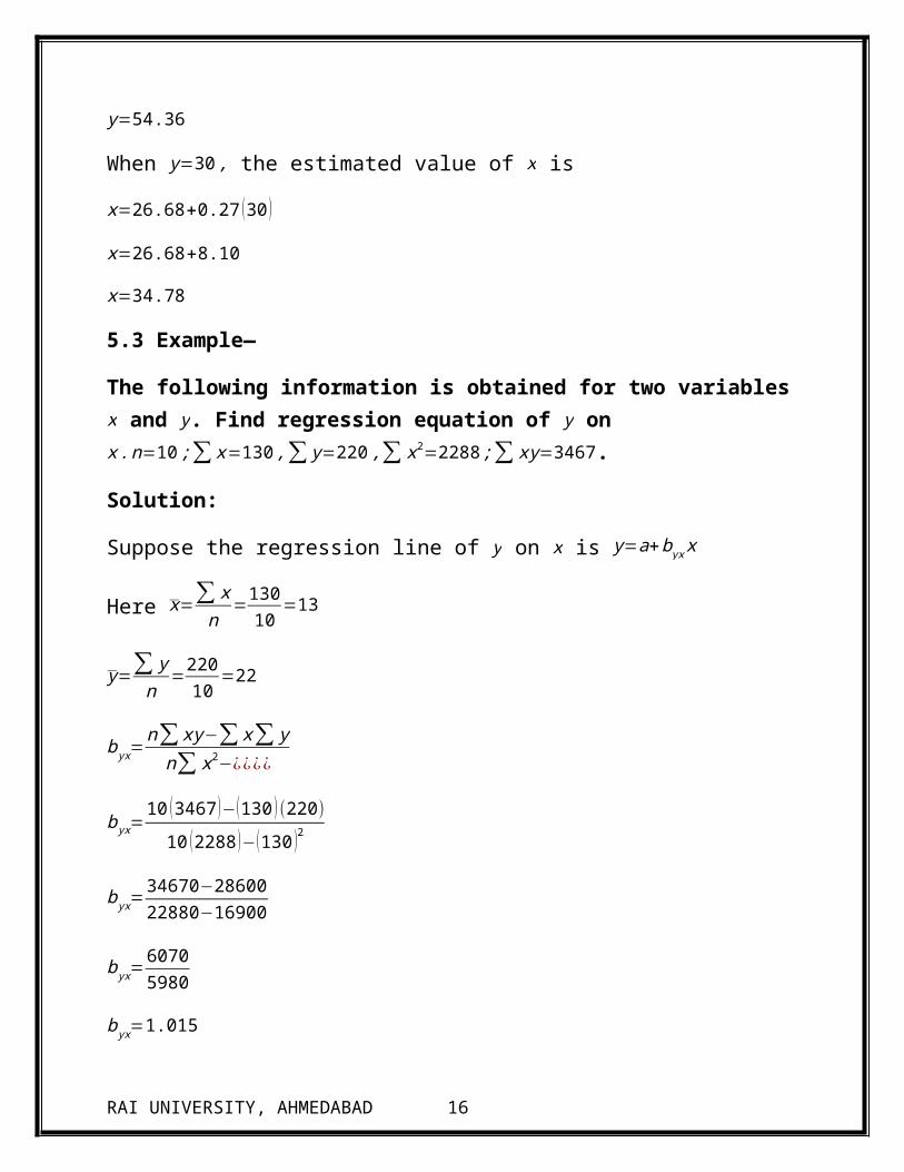
5.3 Example—

The following information is obtained for two variables x and y. Find regression equation of y on x .n=10 ;∑ x=130 ,∑ y=220 ,∑ x2=2288 ;∑ xy=3467.

Solution:

Suppose the regression line of y on x is y=a+b yx x

Here x=∑ x

n=

13010

=13


y=∑ y

n=

22010

=22

b yx=n∑ xy−∑ x∑ y

n∑ x2−¿¿¿¿

b yx=10 (3467 )−(130 )(220)

10 (2288 )−(130 )2

b yx=34670−2860022880−16900

b yx=60705980

b yx=1.015

And a= y−byx x

a=22−1.015 (13)

a=8.805

∴ y=8.805+1.015 x Is the regression line of y on x.

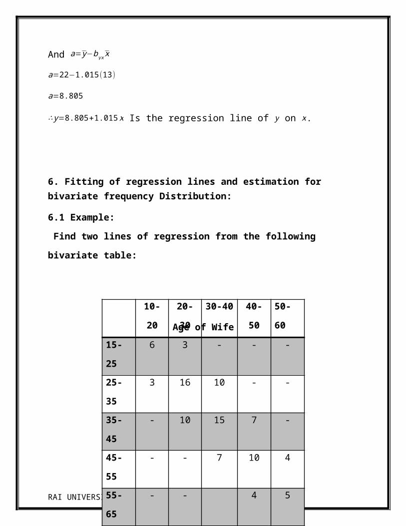
6. Fitting of regression lines and estimation for bivariate frequency Distribution:

6.1 Example:

Find two lines of regression from the following bivariate table:

Age of Wife


10-20 20-30 30-40 40-50 50-60

15-25 6 3 - - -

25-35 3 16 10 - -

35-45 - 10 15 7 -

45-55 - - 7 10 4

55-65 - - 4 5

Age

Of

Husband

Solution:

↓→x

Y

10-20 20-30 30-40 40-50 50-60 f y M.V.

y

v v f v v2 f v fuv

15-25 (24)

6

(6)

3 9 20 -2 -18 36 30

25-35 (6)

3

(16)

16

(0)

10 29 30 -1 -29 29 22

35-45 (0)

10

(0)

15

(0)

7 32 40 0 0 0 0

45-55 (0)

7

(10)

10

(8)

4 21 50 1 21 21 18

55-65 (8)

4

(20)

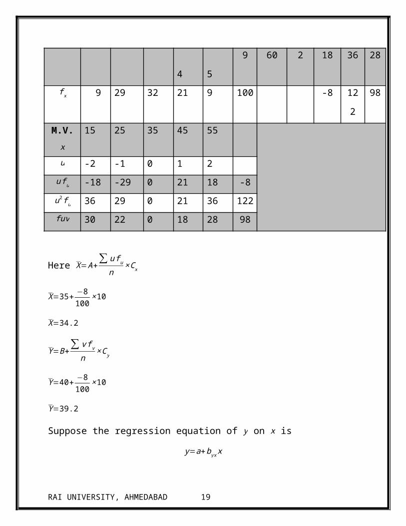
5 9 60 2 18 36 28

f x 9 29 32 21 9 100 -8 122 98

M.V. x 15 25 35 45 55

u -2 -1 0 1 2

u f u -18 -29 0 21 18 -8

u2 f u 36 29 0 21 36 122

fuv 30 22 0 18 28 98


Here X=A+∑ u f un

×C x

X=35+ −8100

×10

X=34.2

Y=B+∑ v f vn

×C y

Y=40+ −8100

×10

Y=39.2

Suppose the regression equation of y on x is

y=a+b yx x

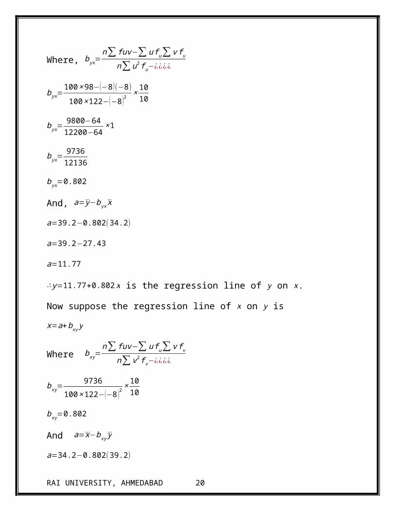
Where, b yx=n∑ fuv−∑ u f u∑ v f vn∑ u2 f u−¿¿¿¿

b yx=100×98−(−8 )(−8)

100×122−(−8 )2×

1010

b yx=9800−6412200−64

×1

b yx=973612136

b yx=0.802

And, a= y−byx x

a=39.2−0.802 (34.2)

a=39.2−27.43

a=11.77

∴ y=11.77+0.802x is the regression line of y on x.

Now suppose the regression line of x on y is


x=a+bxy y

Where bxy=n∑ fuv−∑ u f u∑ v f vn∑ v2 f v−¿¿¿¿

bxy=9736

100×122−(−8 )2×

1010

bxy=0.802

And a=x−bxy y

a=34.2−0.802 (39.2)

a=34.2−31.44

a=2.76

∴ x=2.76+0.802 y is the regression line of x on y.

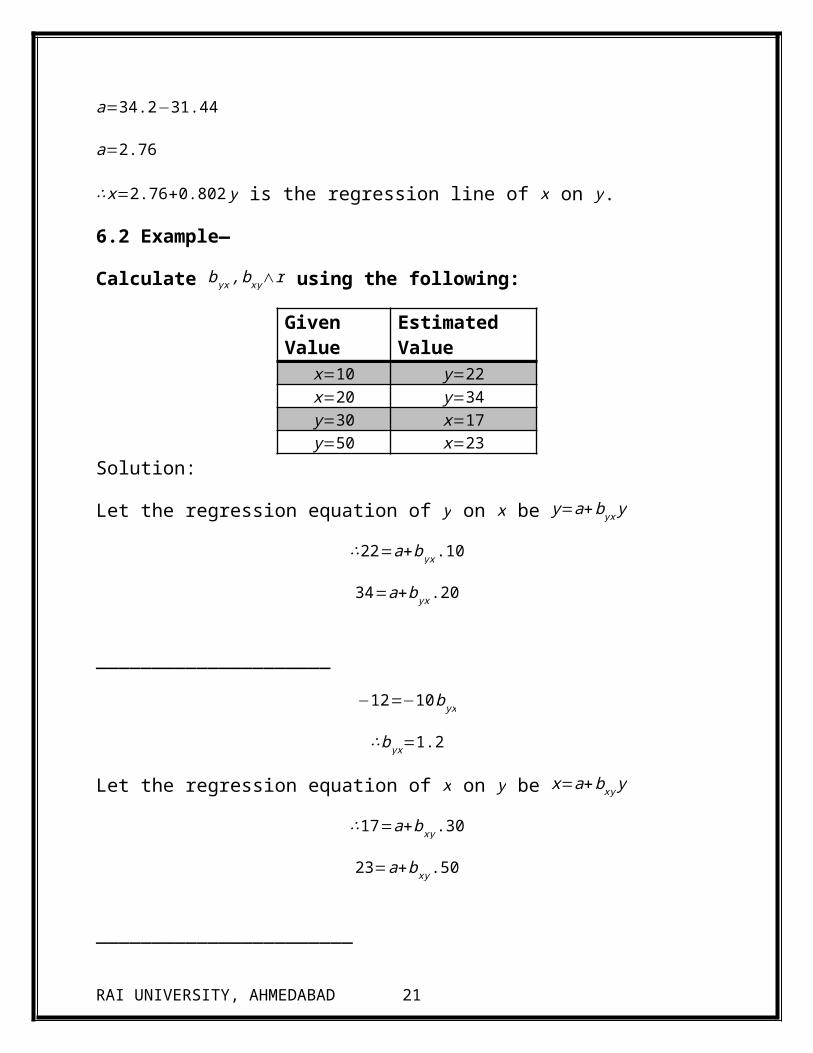
6.2 Example—

Calculate b yx ,bxy∧r using the following:

Given Value Estimated Valuex=10 y=22x=20 y=34y=30 x=17y=50 x=23

Solution:

Let the regression equation of y on x be y=a+b yx y

∴22=a+b yx .10

34=a+byx .20

_____________________

−12=−10b yx

∴b yx=1.2

Let the regression equation of x on y be x=a+bxy y


∴17=a+bxy .30

23=a+bxy .50

_______________________

−6=−bxy .20

bxy=6

20=0.3

Now r=√byx . bxy

r=√ (1.2 )(0.3)

r=√0.36

r=0.6

7.1Advantages of Regression Analysis: 1. The estimates of the unknown parameters obtained from linear least squares

regression are the optimal.

2. Estimates from a broad class of possible parameter estimates under the usual assumptions are used for process modeling.

3. It uses data very efficiently. Good results can be obtained with relatively small data sets.

4. The theory associated with linear regression is well-understood and allows for construction of different types of easily-interpretable statistical intervals for predictions, calibrations, and optimizations.

7.2 Limitations of Regression Analysis:

1. In making estimate from a regression equation, it is important to remember that the assumption is being made that relationship has not changed since the regression equation was computed. Another point worth remembering is that the relationship shown by the scatter diagram may not be the same if the equation is extended beyond the values used in computing the equation.

For example there may be a close linear relationship between the yield of a crop and the amount of fertilizer applied, with the yield increasing as the


amount of fertilizer is increased. It would not be logical, however, to extend this equation beyond the limits of the experiment for it is quite likely that if the amount of fertilizer were increased indefinitely, the yield would eventually decline as too much fertilizer was applied.

Reference Book and Website Name:

1. Statistical Methods by S.P.Gupat2. Business statistics by R.S.Bardwaj3. Business statistics ( B.S. Shah Prakashan)4. www.answers.com/Q/

What_is_the_advantages_and_disadvantages_of_multiple_regression_analysis

5. http://www.biomedware.com/files/documentation/spacestat/Statistics/ Multivariate_Modeling/Regression/regression_line.png


http://www.biomedware.com/files/documentation/spacestat/Statistics/Multivariate_Modeling/Regression/regression_line.png

http://www.biomedware.com/files/documentation/spacestat/Statistics/Multivariate_Modeling/Regression/regression_line.png

http://www.answers.com/Q/What_is_the_advantages_and_disadvantages_of_multiple_regression_analysis



EXERCISE

Q-1. Evaluate the following Questions:

1. Find the equations of regression lines from the following data and also estimate y for x=1 and x for y=4.

x : 3 2 -1 6 4 -2 5 7y : 5 13 12 -1 2 20 0 -3

2. Find regression co-efficients from the following data:

x : 21 22 23 24 25 26 27 28 29 30y : 17 19 19 20 23 24 27 26 28 27

3. Obtain two regression lines from the following bivariate table:

Height Weight90-100 100-110 110-120 120-130


50-55 4 7 5 255-60 6 10 7 460-65 6 12 10 765-70 3 8 6 3

4. The two regression lines are x+2 y−5=0 and 2 x+3 y−8=0 and σ x2=12, find x ,

y,σ y2∧r .



Documents

Course pack unit 5