COVER SHEET

NOTE: Please attach the signed copyright release form at the end of your paper and upload as a

single ‘pdf’ file This coversheet is intended for you to list your article title and author(s) name only This page will not appear in the book or on the CD-ROM

Title: Damage detection using Andrew plots

Authors: Fahit Gharibnezhad ,

Luis E. Mujica , Jose Rodellar

PAPER DEADLINE: **May 15, 2011**

PAPER LENGTH: **8 PAGES MAXIMUM **

SEND PAPER TO: Professor Fu-Kuo ChangOrganizing ChairmanAeronautics and Astronautics DepartmentStanford UniversityDurand BuildingStanford, California 94305, U.S.A.

Tel: 650/723-3466Fax: 650/725-3377E-mail: fkchang@stanford.edu

Please submit your paper in Microsoft Word® format or PDF if prepared in a program other than MSWord. We encourage you to read attached Guidelines prior to preparing your paper—this will ensure your paper is consistent with the format of the articles in the CD-ROM.

--

NOTE: Sample guidelines are shown with the correct margins.Follow the style from these guidelines for your page format.

Hardcopy submission: Pages can be output on a high-grade white bond paper with adherence to the specified margins (8.5 x 11 inch paper. Adjust outside margins if using A4 paper). Please number your pages in light pencil or non-photo blue pencil at the bottom.

Electronic file submission: When making your final PDF for submission make sure the box at “Printed Optimized PDF” is checked. Also—in Distiller—make certain all fonts are embedded in the document before making the final PDF.

ABSTRACT

In current work, Andrew plot is used as a new index to detect any probable damage in the structure. At the first step, using piezoelectric actuators and sensors, appropriate lamb wave is propagated and received through the structure. Then Principal Component Analysis is applied to the recorded data and prepares necessary data for Andrew curves. Andrew plots are depicted based on calculated principal components. It has been shown that comparing Andrew curves from baseline, structure without damage, with current statues of structure can identify any probable damages in the structure.

INTRODUCTION

In recent years, there has been an increasing awareness of the importance of damage prognosis systems in aerospace, civil and mechanical structures because of huge expenses that are spent every year maintaining and repairing buildings, bridges, aircraft, railroads, and other infrastructure. One such technique that has gained much attention in the research and industrial communities over the past two decades is structural health monitoring [1].Structural health monitoring (SHM) is a damage detection technique that involves placing intelligent sensors on a structure, periodically recording data from the sensors, and using statistical methods to analyze the data in order to assess the condition of the structure. The field of SHM developed through the combination of nondestructive evaluation (NDE) methods and novel sensing and actuation techniques to create intelligent monitoring systems permanently installed on structures. To achieve this aim there are several potentially useful techniques, and their applicability to a particular situation depends on the size of critical damage admissible in the structure. The development of practical monitoring systems that can be implemented on real world structures faces several design challenges including the development of stand alone vibration sensors/actuators, effective damage detection algorithms, and low power wireless transmission systems. Some SHM systems currently being developed include vibration actuation, data acquisition, data processing, and data transmission capabilities all in stand alone wireless sensor units attached at various locations along a structure. All of these techniques follow the same general procedure: the pristine structure is excited using appropriate actuators and the dynamical response is sensed at different locations throughout the structure. Any damage will change this vibrational

response, as well as the transient by a wave that is spreading through the structure. Several methods have been used to obtain this vibrational response, for instance: using fiber-optic or piezoelectric transducers. In the next step, necessary data is collected and then, the state of the structure is diagnosed by means of the processing of these data. Correlating the signals to detect, locate and quantify these changes is a very complex problem, but very significant progresses have been recently reported in conferences new scientific journals and books. Among these methods, developing techniques using or based on Principal Component Analysis (PCA) for feature discrimination has been considered recently [2]. PCA is the most useful tool in dimensional reduction. The central idea of PCA is to reduce the dimensionality of a data set consisting of a large number of interrelated variables, while retaining as much as possible of the variation present in the data set. This is achieved by transforming to a new set of variables, the principal components (PCs), which are uncorrelated, and which are ordered so that the first few retain most of the variation present in all of the original variables. If the data compression is sufficient, the large number of variables is substituted by a small number of uncorrelated latent factors, called principal components (PCs), which can explain sufficiently the data structure. Obtained PCs could be used as feed for other methods in SHM field. For instance, Andrew plots, as a tool to graphically interpret multivariate data and classify them, could be used as an index to detect probable damages in the structure using PCA. Experimental results in current work, confirm this claim.This paper is structured in the following way: First Andrew plots is introduced in more details. Its properties and abilities such as case classification is reviewed. Then the strategy to use Andrew plots based on PCA is explained. In next section, the experimental setup is presented. then the algorithm to detect damages using Andrew plots and PCA is scrutinized and result are presented. Finally, the obtained results are summarized in conclusion.

ANDREW PLOTS

Graphical representation of multivariate data has been an important issue in exploratory data analysis. Most data that are collected are multivariate in nature, and much of them can be regarded as continuous. In the initial stages of analysis, graphic displays can be used to explore the data, but for multivariate data, traditional histograms or two or three-dimensional scatter plots may miss complex relationships that exist in the data set. A number of methods for graphically displaying multivariate data have been suggested. One of the most appealing methods is that of Andrews Plots[?].Andrews Plots provide a means for the simultaneous display of several continuous variables. For a multivariate observation y=¿ Andrew suggests a representation of this multivariate point by a curve in argument t (−π ≤t ≤ π ¿

f y (t)=y1

√2+ y2 sin(t )+ y3cos (t )+ y4 sin (2t )+ y5cos (2 t)+… (1)

In a two-dimensional space. The coefficient of y1 , y2 ,… are nothing but the terms in the Fourier series. By storing them in a column vector

a (t)=¿ (2)

we can write f y (t)=a(t) y thereby identifying f y (t) as a particular linear combination y for a fixed t . Thus for a given t 0 , (t 0 , f y (t 0)) represents a point on the curve, and by varying t between −π and π an Andrews curve is obtained as a collection of all such points. Corresponding to n different multivariate observations, there will be n different Andrews curves. A plot consisting of such curves is called an Andrews plot.

Classifying cases with Andrew PlotsAndrews Plots can be used as a technique for classifying observations into groups. Where unknown grouping of cases exists within a data set, an Andrews Plot can be used to discover this effect. Cases within one group will have similar patterns of values for the variables used in the Andrews Plot, and similar curves will be produced for these cases. Cases in a second group will have a different profile of values for the variables from those in the first group, and thus the curves produced for this second group will show a different pattern from those for the first group.Andrews Plots can also be used to allocate a case to one of a number of groups that are known to exist in the data set.Curves for cases whose grouping is known are created and then the curve for the unknown case superimposed. The unknown case is allocated to the group whose set of curves its own curve most closely matches [4].

Andrews plots and Principal Components

One of the major shortcoming of Andrews plots is that while they are able to preserve the distance and the average, they are not order preserving. In other words, the technique places greater weight on those variables listed first (e.g., y1 , y2) and less weight on variables listed later (yn−1 , yn). It is thus recommended that principal components of the original data be produced and used in the order reflecting their importance, unless there is a natural ordering that can be used. Consequently, their shapes, patterns, clustering, etc., may be affected by interchanging the coefficients of the terms in the Fourier series. Mathematically, if y¿ is a permutation of y, then f y

¿ (t)=a(t) y¿ and f y (t)=a(t ) y will represent different curves and their shapes and/or specific patterns may be drastically altered or get hidden. As noted by Andrews(1972), since low frequencies (large periods) are more readily caught by human eyes than the high frequencies, it is useful to associate the most important variables with high periods and thus arrange the variables in a multivariate vector y by the decreasing order of their importance. Due to mentioned reason , Principal components could be a good solution to arrange the vector y by the decreasing order of their importance.y=¿. Imagine the data in a matrix form of Y n×m containing information from n experimental trials and m sensors. Since physical variables have different magnitudes and scales, each data-point is scaled using the mean of all measurements of the sensor at the same time and the standard deviation of all measurements of the sensor. Once the variables are normalized the covariance matrix C y calculated as follows:

C y=1n−1

Y T Y (3)

C y is a square symmetric matrix (n×n) that measures the degree of linear relationship within the data set between all possible pairs of variables (sensors). The subspaces in PCA are defined by the eigenvectors and eigenvalues of the covariance matrix as follow:

C yP=P Λ (4)

Where the eigenvectors of C y are the columns of P and the eigenvalues are the diagonal terms of Λ (the off-diagonal terms are zero). Columns of matrix P are sorted according to the eigenvalues by descending order and they are called the Principal Components (PCs) of the data set. The eigenvector with the highest eigenvalue represents the most important pattern in the data with the largest quantity of information. Choosing only a reduced number r of principal components, those corresponding to the first eigenvalues, the reduced transformation matrix could be imagined as a model for the structure. Geometrically, the transformed data matrix T (score matrix) is the projection of the original data over the direction of the principal components P.

Y ♦=YP (5)

now Andrew plot can be created based on the ordered data as f y (t)=a(t) y♦.

Alternatives for Andrew plots

Several authors, including Andrews himself, have suggested variations to the vector of functions used in Andrews plots. In this work three different alternative for Andrew plots are used as below. Their similarities and differences in distinguishing damaged patterns from non damaged would be discussed. mentioned alternatives are numerated as below. Equation (6) is original Andrew plot [3] and (7),(8) and (9) are from [5],[6] and [7] respectively.

f y(1)(t )=

y1

√2+ y2sin (t)+ y3 cos(t )+ y4 sin(2 t)+ y5 cos(2 t)+…−π≤ t ≤ π

(6)

f y(2)(t )= y1 cos(t)+ y2 cos (√2 t)+ y3 cos (√3 t )+ y4 cos(√4 t)+…−π ≤ t ≤π

(7)

f y(3)(t )= y1 sin(t)+ y2 cos(t )+ y3sin (2t )+ y4 cos(2 t)+…−π≤ t ≤ π (8)

f y(4 )(t)= 1

√2{ y1+ y2(sin( t)+cos (t))+ y3(sin(t)−cos(t ))+ y4 (sin(2 t)+cos (2 t))+…}

(9)

EXPERIMENTAL SETUP

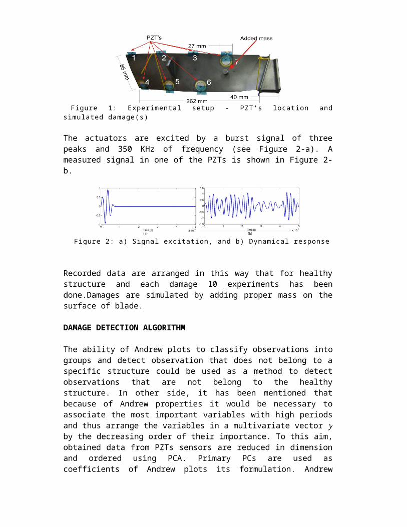
This specimen is a turbine blade of a commercial aircraft.It could be determined that the blade is manufactured by a homogenous material with a similar density like titanium (3.57 g/ml). Figure 1 shows the dimension of blade.Seven PZT sensors are distributed over the surface to detect time varying strain response data.Three of the sensors are on one face and four on the other face as can be seen in Figure 1.To alleviate the influence of environment conditions and isolate the experiments from environmental conditions the blade is suspended by elastic ropes.

Figure 1: Experimental setup - PZT's location and simulated damage(s)

The actuators are excited by a burst signal of three peaks and 350 KHz of frequency (see Figure 2-a). A measured signal in one of the PZTs is shown in Figure 2-b.

Figure 2: a) Signal excitation, and b) Dynamical response

Recorded data are arranged in this way that for healthy structure and each damage 10 experiments has been done.Damages are simulated by adding proper mass on the surface of blade.

DAMAGE DETECTION ALGORITHM

The ability of Andrew plots to classify observations into groups and detect observation that does not belong to a specific structure could be used as a method to detect observations that are not belong to the healthy structure. In other side, it has been mentioned that because of Andrew properties it would be necessary to associate the most important variables with high periods and thus arrange the variables in a multivariate vector y by the decreasing order of their importance. To this aim, obtained data from PZTs sensors are reduced in dimension and ordered using PCA. Primary PCs are used as coefficients of Andrew plots its formulation. Andrew curves are calculated for each observation and finally all curves are depicted in a same plot to demonstrate the result. Using less number of PCs generate smoother function and

more proper figure to distinguish the damages from non damaged structure. In this work, moreover, to have a better view curves were evaluated for values of t from −2π to 2π a total range of 4 π instead of original period. Equation (6) is re written using PCs as below

f y(1)(t )= pc1

√2+ pc2sin (t)+ pc3 cos (t)+ pc4 sin(2 t)+ pc5cos (2 t)+…

(10)

Figure 4 shows the result of Andrew plots for 2 different damage with non-damaged data using first five Principal Components. As it has been shown, there are three different patterns. the pattern depicted in green is data from non-damaged structure and other two patterns, depicted in red and blue, are related to damage 1 and damage 2 respectively. According to the figure, different patterns are distinguished clearly from each other. This property not only can be used to detect probable damages in a structure but also could classify any type of damages. To do this, enough experiment should be done to create a baseline from the healthy structure using Andrew plot and PCA. after collecting enough data from the non-damaged structure, available pattern could be used as baseline to show that whether the next observation is belong to the healthy structure pattern or there is a probable damage in the structure.

Figure 4: Andrew plots, non-damage with 2 different damages Figure 3???It is obvious if instead of first five PCs , the first seven PCs would be chosen the figures will be less smooth as the higher frequencies are included. Figure 5 confirm this idea.

Figure 5: Andrew plots with classical PCA, first 17 Principal Components

Other alternatives for original Andrew plots also are used to see if they are able to distinguish the patterns of damaged structure from non-damaged. Figure 6 shows the result of equation (7). According to the figure, in this plot all functions belong to a certain group intersect each other in the certain point. In other words, using this property any new data could be categorized as non-damaged, known damaged pattern or new type of damage.Therefore, both damage detection and identification are satisfied in this method.

Figure 6: Gnanadesikan (left) and Paranjape(right) plot Next figure is belong to equation (8) where the same behavior has been seen when functions belong to the equal pattern meet each other in the same point (Figure 6).The last one (figure 8) is depicted using equation (9) the behavior of this function is very close to the original Andrew plot.

Figure 8: Ravindra plot

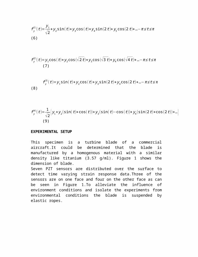
Figure 9: Different alternatives for Andrew plots

Finally , figure 9 shows all alternatives for Andrew plots in the same position.

CONCLUSIONS

Andrew plot as graphical representation of multivariate data could be used as an index to identify any probable damage in the structure.As the order of coefficients of terms are very important, these coefficients should be rearranged depending on their importance.PCA can be used in this manner for bot ordering and reducing the dimensionality.Obtained curves show that each observation is belong to which group.Therefore,using depicted figures any damage can be separated from healthy observation in which not only detect the damage but also clarify the type of damage.Results from the experiments confirm this idea where two different simulated damages are detected and classified.ACKNOWLEDGMENTS

This work has been supported by the "Ministerio de Ciencia e Innovaciуn'' in Spain through the coordinated research project DPI2008-06564-C02-02, and the "Formacion de Personal Investigador" FPI doctoral scholarship. The authors would like to thank the support from "Universitat Politйcnica de Catalunya" and "Universidad Politйcnica de Madrid". We are also grateful to Professor Alfredo Gьemes and Dr. Antonio Fernandez for his valuable suggestions and ideas during the experimental phase. REFERENCES

[1]S.Anton, Baseline-Free and Self-Powered Structural Health Monitoring,Ph.D. dissertation, 2008

[2] L. E. Mujica, J. Rodellar, a.Fernandez, and a. Guemes,Q-statistic and T2-statistic PCA-based measures for damage assessment in structures,Structural Health Monitoring,Nov. 2010. [3] D. Andrews, Plots of high-dimensional data,Biometrics, vol. 28, no. 1, pp.125 136, 1972[4] N. Spencer, Investigating data with Andrews plots, Social science computer review, vol. 21, no. 2, p. 244, 2003[5] R. Gnanadesikan, Methods for Statistical Data Analysis of Multivariate Ob-servations, 2nd ed. Wiley,New York, 1997.[6] S. K. S. Paranjapea, Use, of andrews’ function plot technique to construct control curves for multivariate process,Communications in Statistics Theory and Methods, vol. 13, pp. 2511 2533, 1984.[7] R. Khattree, Andrews plots for multivariate data: some new suggestions and applications, Journal of Statistical Planning and Inference, vol. 100, no. 2, pp. 411-425, Feb. 2002