Crab Flares and the Nebular Variability

Demosthenes Kazanas

NASA/GSFC, Code 663

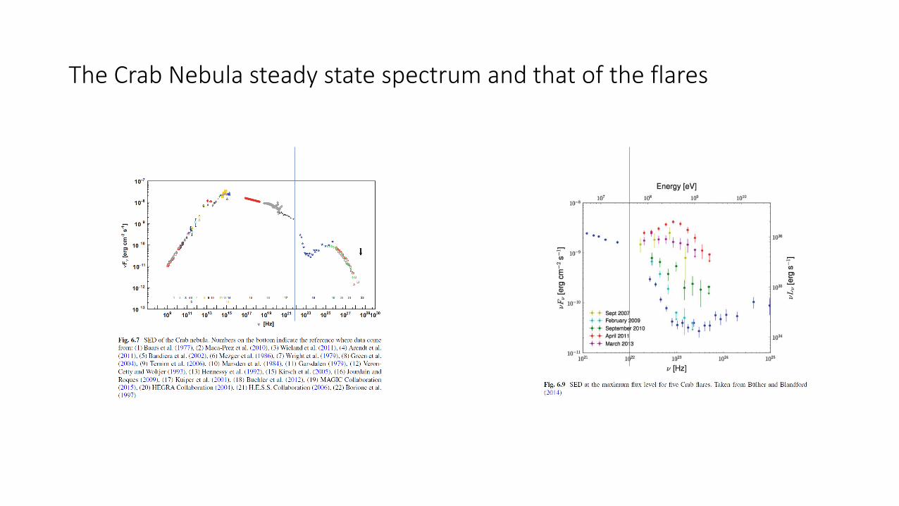
The Crab Nebula steady state spectrum and that of the flares

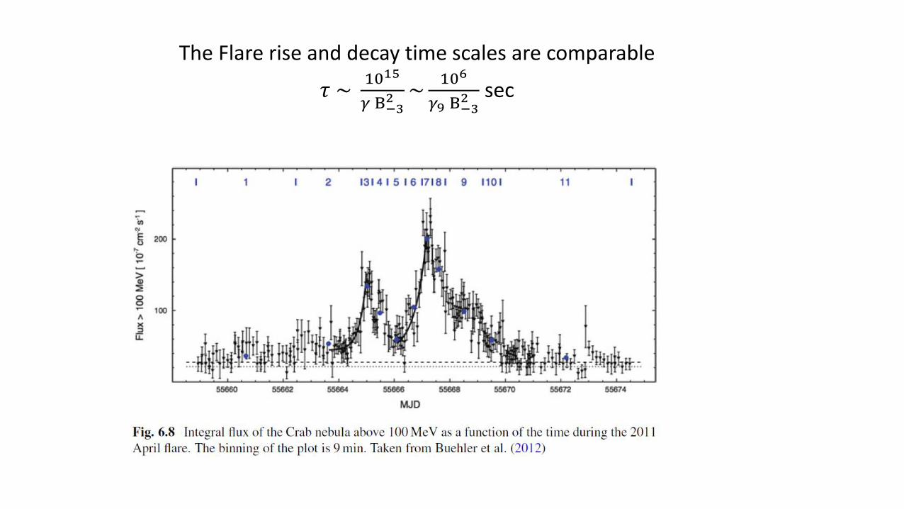
The Flare rise and decay time scales are comparable

𝜏 ~1015

𝛾 Β−32 ~

106

𝛾9 Β−32 sec

Some facts related to the flares

• If the B-field drops linearly from the pulsar LC (~108 cm) to the MHD shock (~1017

cm), the field at the shock should be B ~ 10-3 B-3 .

• The spectra of the flares are an extrapolation of the nebular spectrum, likely due to the same process, i.e. synchrotron.

• The observed energies are larger than the (B-independent) maximum synchrotron photon energy of particles accelerated in a shock, i.e. E > mec

2/α ~ 70 MeV.

• The flare particles are not accelerated by shock acceleration!

• There have been suggestions of linear increase of the MHD wind Γ with distance (IC + DK 2003) to Γ ~ 109, close to that needed to explain the flares (with B ~ 10-3

B-3 G, νs ~ 4 103 B-3 γ2 ~ 1022 Hz➔ γ ~ 0.5 x 109 ).

• If the pulsar wind field lines are good conductors, the polar cap potential (V ~ 1016 Volt, γ ~ 1010) is available for discharge should the appropriate field lines get sufficiently close.

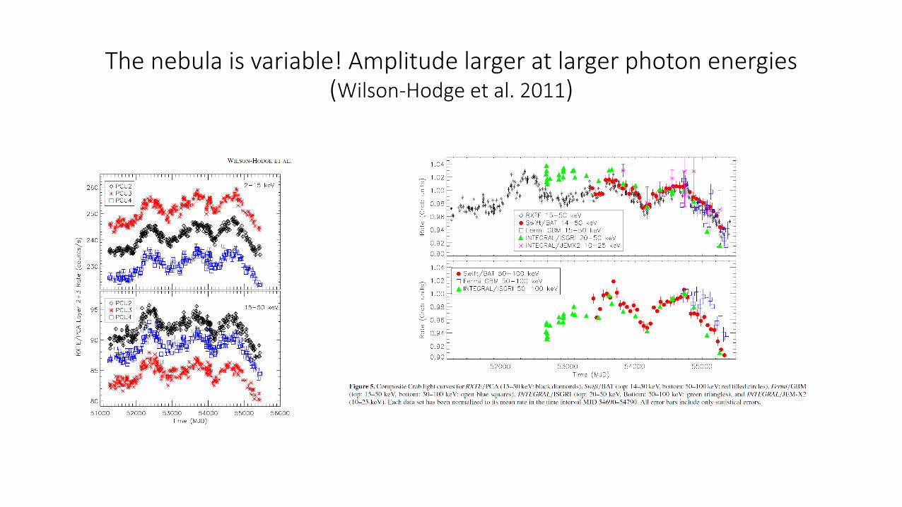
The nebula is variable! Amplitude larger at larger photon energies (Wilson-Hodge et al. 2011)

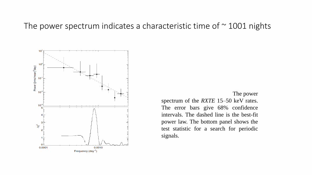
The power spectrum indicates a characteristic time of ~ 1001 nights

The power

spectrum of the RXTE 15–50 keV rates.

The error bars give 68% confidence

intervals. The dashed line is the best-fit

power law. The bottom panel shows the

test statistic for a search for periodic

signals.

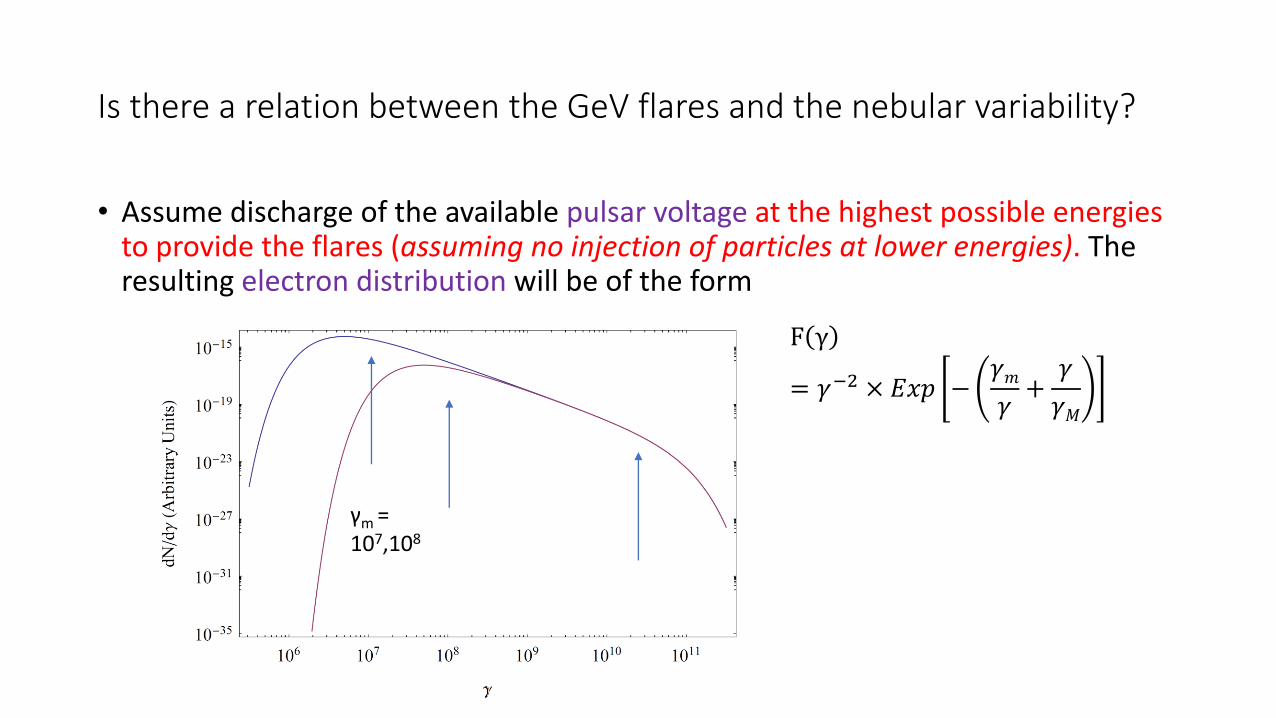
Is there a relation between the GeV flares and the nebular variability?

• Assume discharge of the available pulsar voltage at the highest possible energies to provide the flares (assuming no injection of particles at lower energies). The resulting electron distribution will be of the form

F γ

= 𝛾−2 × 𝐸𝑥𝑝 −𝛾𝑚𝛾+

𝛾

𝛾𝑀

γm = 107,108

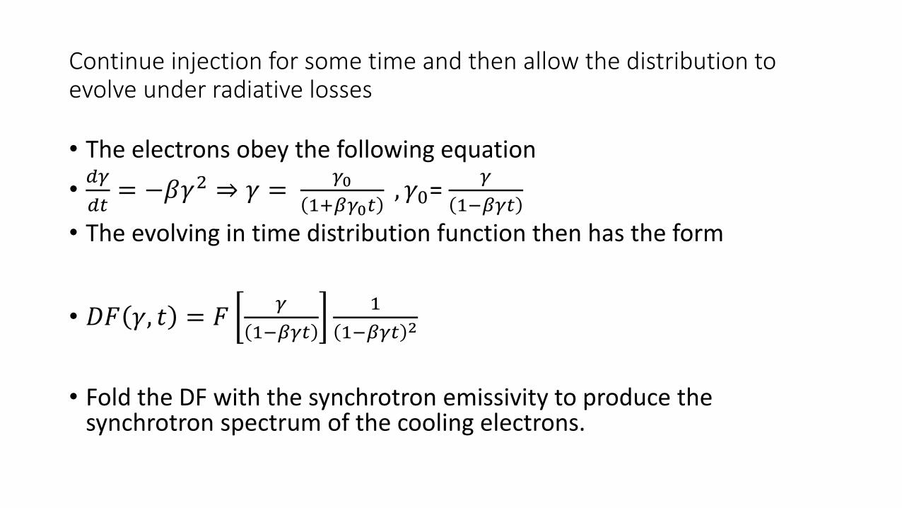
Continue injection for some time and then allow the distribution to evolve under radiative losses

• The electrons obey the following equation

•𝑑𝛾

𝑑𝑡= −𝛽𝛾2 ⇒ 𝛾 =

𝛾0

1+𝛽𝛾0𝑡, 𝛾0=

𝛾

1−𝛽𝛾𝑡

• The evolving in time distribution function then has the form

• 𝐷𝐹 𝛾, 𝑡 = 𝐹𝛾

1−𝛽𝛾𝑡

1

1−𝛽𝛾𝑡 2

• Fold the DF with the synchrotron emissivity to produce the synchrotron spectrum of the cooling electrons.

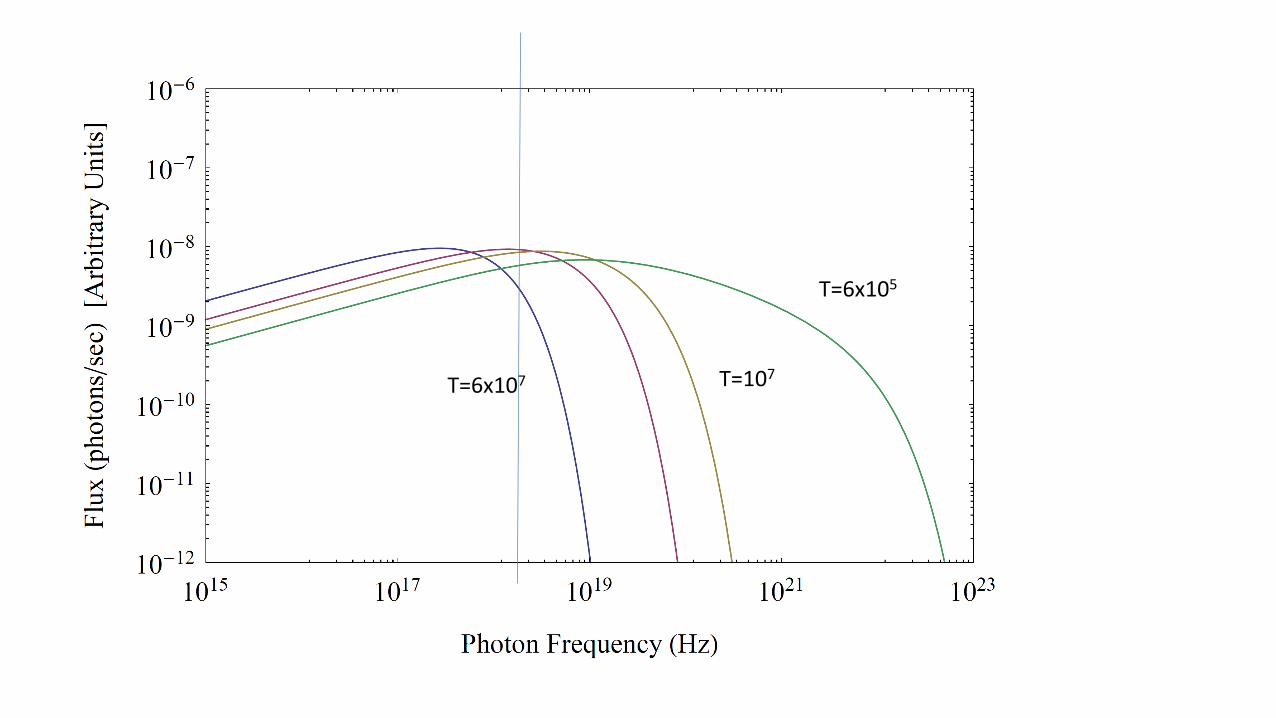
T=6x105

T=107T=6x107

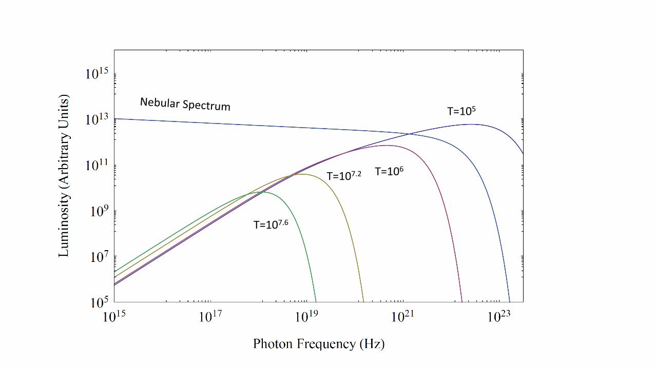
T=105

T=106T=107.2

T=107.6

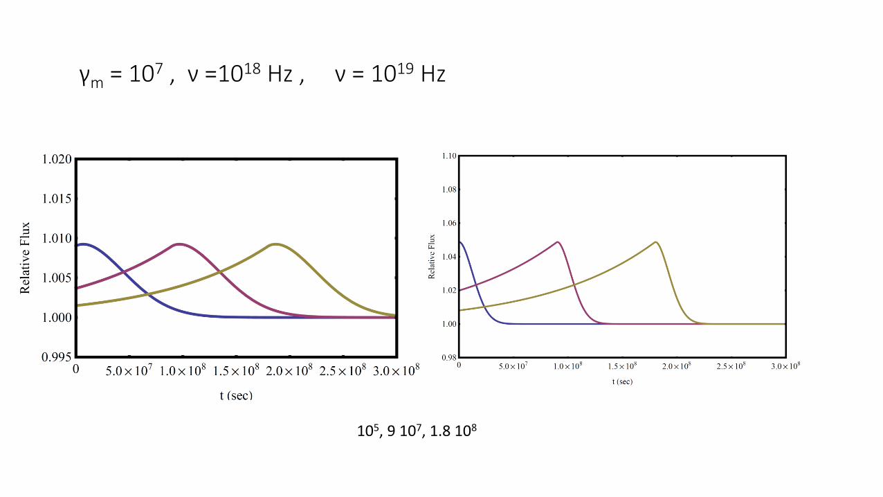
γm = 107 , ν =1018 Hz , ν = 1019 Hz

105, 9 107, 1.8 108

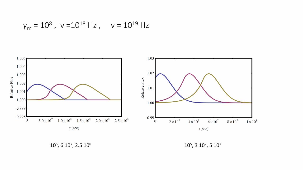
γm = 108 , ν =1018 Hz , ν = 1019 Hz

105, 6 107, 2.5 108 105, 3 107, 5 107

Conclusions

• There are indications that the Crab flares give rise to the Crab Nebula fluctuations (of relative amplitude ~<4%) observed by a number of spacecraft.

• The long variation periods (~ 1001 days), seen at Swift – BAT, INTEGRAL, Fermi-GBM, along with their observed relative amplitude of the oscillations can constraint significantly the properties of the injected particles, assuming injection at the Crab flares and subsequent cooling.

• There are caveats in the oscillation interpretation which have not been considered so far (e.g. cooling in a B-field much weaker than that of particle injection; injection with a sufficiently flat particle spectrum i.e. ~ γ-2), which may help the reconcile observed X-ray oscillation amplitudes and time scales with those of flare occurrences.

• Thank you!