Embed Size (px)
Citation preview

CRANFIELD INSTITUTE OF TECHNOLOGY
P. J. MODENESI
Statistical Modelling of the Narrow GapGas Metal Arc Welding Process
School of Industrial Science
PhD Thesis
CRANFIELD INSTITUTE OF TECHNOLOGY
SCHOOL OF INDUSTRIAL SCIENCE
PhD THESIS
Academic year 1989-90
P. J. MODENESI
Statistical Modelling of the Narrow GapGas Metal Arc Welding Process
Supervisor: R. L. Apps
April 1990
This thesis is submitted in partial submission for the degree ofPhD

ABSTRACT
The J-laying technique for the construction of offshore pipelines requires a fast weldingprocess that can produce sound welds in the horizontal-vertical position. The suitability ofnarrow gap gas metal arc welding (NG-GMAW) process for this application was previouslydemonstrated.
The present programme studied the influence of process parameters on the fusioncharacteristics of NG-GMA welding in a range of different shielding gas compositions andwelding positions. Statistical techniques were employed for both designing the experimentalprogramme and to process the data generated. A partial factorial design scheme was used toinvestigate the influence of input variables and their interaction in determining weld beadshape. Modelling equations were developed by multiple linear regression to representdifferent characteristics of the weld bead. Transformation of the response variable based onthe Cox-Box method was commonly used to simplify the model format. Modelling resultswere analysed by graphical techniques including surface plots and a multiplot approach wasdeveloped in order to graphically assess the influence of up to four input variables on thebead shape.
Conditions for acceptable bead formation were determined and the process sensitivity tominor changes in input parameters assessed. Asymmetrical base metal fusion in horizontal-vertical welding is discussed and techniques to improve fusion presented.
At the same time, the interaction between the power supply output characteristic and the beadgeometry was studied for narrow gap joints and the effect of shielding gas composition onboth process stability and fusion of the base metal was assessed. An arc instability mode thatis strongly influenced by arc length, power supply characteristic and shielding gascomposition was demonstrated and its properties investigated. An optimized shielding gascomposition for narrow gap process was suggested.

ACKNOWLEDGMENTS
I would like to express my gratitude to Mr. J. H. Nixon for his guidance and assistanceduring this project and to Prof. R. L. Apps for his initial guidance.
I would also like to thank all my friends and colleagues in the Welding Group, speciallyCelso and Sadek, for their support and encouragement.
The financial support of CAPES and Universidade Federal de Minas Gerais, Brazil, isacknowledged.
Finally, I wish to dedicate this work to Giovana whose support made it possible.
CONTENTS
LIST OF FIGURES (i)
NOTATION (viii)
1 - CHAPTER 1: Introduction 1
2 - CHAPTER 2: Literature survey 3
2.1 - Construction of submarine pipelines 4
2.2 - Gas metal arc welding 62.2.1 - Introduction 62.2.2 - The welding arc 72.2.3 - Metal transfer 102.2.4 - Wire melting rate 122.2.5 - Shielding gases 152.2.6 - Equipment and process control 17
2.2.6.1 - Power supplies 172.2.6.2 - Control aspects in GMAW 18
2.3 - Narrow gap welding 202.3.1 - Introduction 202.3.2 - Narrow gap GMAW 22
2.4 - Modelling of the weld bead shape 262.4.1 - Introduction 262.4.2 - Mathematical modelling 27
2.4.2.1 - Theoretical approach 282.4.2.2 - Empirical approach 30
2.4.3 - Statistical design of experiments 322.4.3.1 - Introduction 322.4.3.2 - Factorial design 342.4.3.3 - Regression analysis 36
Tables 41Figures 47
3 - CHAPTER 3: Equipment and materials 61
3.1 - Power supplies 623.1.1 - Transarc Fronius 500 623.1.2 - GEC (AWP) M500 62

3.2 - Wire feed unit 62
3.3 - Welding torch 62
3.4 - Test rig 63
3.5 - Gas mixer and analyser 63
3.6 - Photograph 64
3.7 - Current and voltage measurement 64
3.8 - Metallographic equipment 64
3.9 - Weld bead measurement 64
3.10 - Data analysis 65
3.11 - Materials 653.11.1 - Filler wire 653.11.2 - Base material 653.11.3 - Shielding gases 65
3.12 - Narrow gap welding specimen 66
Tables 67Figures 69
4 - CHAPTER 4: Research programme 72Figure 74
5 - CHAPTER 5: Process modelling 75
5.1 - Experimental procedure 765.1.1 - Design of the experiments 765.1.2 - Initial welding trials 775.1.3 - Modelling steps 775.1.4 - Complementary trials 78
5.2 - Experimental results 785.2.1 - Pulsed current parameters 785.2.2 - Arc length 795.2.3 - Weld bead characteristics 805.2.4 - Complementary trials 82
5.3 - Modelling procedure 82
5.4 - Modelling results 85
Tables 87Figures 116
6 - CHAPTER 6: Analysis of results and discussion 132
6.1 - Assessment of experimental and modelling techniques 1336.1.1 - Experimental design 1336.1.2 - Data analysis 135
6.2 - Bead characteristics 1366.2.1 - Bead parameters related with wire fusion 1376.2.2 - Bead parameters related with plate fusion 139
6.2.2.1 - Introduction 1396.2.2.2 - Modelling results 140
6.2.3 - Bead parameters related with both plate and wire fusion 141
6.3 - Graphical representation of process behaviour 142
6.4 - Horizontal-vertical welding 146
6.5 - Summary 148
Tables 149Figures 151
7 - CHAPTER 7: Shielding gas/process optimization 171
7.1 - Introduction 172
7.2 - Arc length dependent process instability 1727.2.1 - Initial experiments 1737.2.2 - Tests with constant voltage 1737.2.3 - Tests with constant current 1747.2.4 - Tests with pulsed current 175
7.3 - Fusion characteristics 176
7.4 - Power supply characteristics 177
7.5 - Discussion 1797.5.1 - Arc length dependent stability 179
7.5.1.1 - Introduction 1797.5.1.2 - Phenomenological aspects 180

7.5.1.3 - Tentative mechanism 1847.5.2 - Shielding gas/process optimization 187
7.5.2.1 - Shielding gas 1877.5.2.2 - Power supply characteristics 1887.5.2.3 - Steady and pulsed current 189
Tables 190Figures 200
8 - CHAPTER 8: Conclusions 233
9 - CHAPTER 9: Recommendations for further work 236
10 - REFERENCES 238
Appendix A 252
Appendix B 255
Appendix C 271
i
LIST OF FIGURES:
Chapter 2:
2.1 Illustration of the S curve pipelaying system (Fennel 1986).
2.2 Illustration of the J curve pipelaying system (Fennel 1986).
2.3 Schematic representation of the GMAW process.
2.4 Schematic representation of the voltage distribution along an arc.
2.5 Common metal transfer modes in GMAW.
2.6 Idealised representation of the effect of current and voltage on metal transfermode (based on Matumoto 1982).
2.7 Conditions for one pulse-one drop obtained from different authors: (1)Ueguri(1985), (2) Allum (1983), (3) Foote (1986) and (4) Smati (1986).
2.8 Classification of NGW processes in Japan (Nomura and Sugitani 1984).
2.9 Classification of NGW processes (Malin 1987).
2.10 Welding costs as a function of joint thickness for different welding processes:(1)Single wire SAW, (2)single wire SAW-NG, two passes per layer, (3)sametechnique but with tandem wires, (4)tandem wires SAW-NG, one pass per layer,(5)single wire SAW-NG, one pass per layer, (6)GMAW-NG, and (7) ESW(Manzoli and Caccia 1989).
2.11 Effect of gas flow rate and plate thickness on blow hole formation (Kurokawa etal.).
2.12 Effect of voltage on process stability and bead formation (Malin 1987).
2.13 Classification of models (Gordon 1978).
2.14 Two dimensional model of the weld pool (Nishiguchi et al. 1975).
2.15 Generalised representation of fusion characteristics in pulsed GMAW (Quintino1986).
2.16 Outline of experimental method for tolerance box technique: (a)Initial factoriallattice; (b)focused experimental lattice (acceptable welds: dark circles);(c)experimentally determined boudary positions; (d)boundary lines andassociated defects (McGlone 1980).
2.17 Squematic representation of an experiment.

ii
2.18 Geometric representation of a two-level factorial design for k = 3.
2.19 Example of application of the normal distribution plot to access the significantfactors in a 25-1 factorial experiment. Data from Raveendra and Parmar (1987).X1, voltage, X2, current, X3, welding speed, X4, groove angle, and X5, standoff.Response: bead width in SAW.
Chapter 3
3.1 Calibration curve for the ESAB A10-MEC44 wire feeder.
3.2 Welding rig (used with the GEC (AWP) M500 power supply).
3.3 Calibration curve for the welding table.
3.4 Schematic diagram of the welding rig.
3.5 Gas mixer.
3.6 Diagram of narrow gap welding specimen.
Chapter 4
4.1 Flowchart of the experimental programme.
Chapter 5
5.1 Effect of the software filtering routine on the welding current trace. Top: originaldata. Bottom: filtered data.
5.2 Procedure used in the software to calculate current peak and base parameters.
5.3 Definition of bead, deposited, lateral penetration and axial penetration areas.
5.4 The definition of maximum arc action height (hmax) for weld beads with (a) andwithout (b) undercutting. Undercutting area (Au) is also shown in (b).
5.5 Schematic representation of the dificulty in using undercutting area to model theundercutting tendency in a weld process.
5.6 Convention adopted to define and measure lateral lack of fusion. (a)Transversesection of a welded specimen. Magnified views of the region enclosed by thecircle in (a), with the estimated values of lf, are shown in (b) and (c), for weldbeads with positive and negative lack of fusion respectively.
5.7 Weld bead macrosections of horizontal-vertical welds performed with weldingspeeds of (a)6mm/s and (b)10mm/s. Magnification: 6X.
iii
5.8 Definitions of upper and lower side lateral penetration areas (a), and upper andlower axial penetration area (b).
5.9 Variabillity of bead area (At), deposited area (Ad) and lateral penetration area(Ap) along the bead length for narrow gap specimens welded with Ar-5 (a) andHe-1 (b), experimental step S0.
5.10 Macrosections of multipass downhand (a) and horizontal-vertical (b) welds. 5X.
5.11 Schematic representation of a linear model being used to represent locally amore complex relationship E(y) between a response y and the predictors x1 andx2.
5.12 Graphical procedure to determine the confidence interval on t.
5.13 Variation of the F ratio, R2 and MSet statistics with the transformation factor tfor bead area models.
5.14 Variation of the F ratio, R2 and MSet statistics with the transformation factor tfor lateral penetration area models.
5.15 Variation of the F ratio, R2 and MSet statistics with the transformation factor tfor mean bead height models.
5.16 Variation of the F ratio, R2 and MSet statistics with the transformation factor tfor H/W ratio models.
5.17 Predicted value plots of MODEL A equations for some responses of S1-B1.
5.18 Predicted value plots of MODEL A equations for some responses of S1-B2.
5.19 Predicted value plots of MODEL A equations for some responses of S2-B1.
5.20 Surface plots for predicted production time in experimental blocks (a)S1-B1,(b)S1-B2 and (C)S2-B1.
5.21 Surface plots for lateral penetration area in experimental blocks (a)S1-B1,(b)S1-B2 and (C)S2-B1. Gap: 7mm, welding speed: 7mm/s.
5.22 Surface plots for predicted (a)voltage and (b)arc length in experimental blocks(a)S1-B1.
5.23 Surface plots for predicted lack of fusion in experimental blocks (a)S1-B1,(b)S1-B3 and (C)S2-B1. Gap: 7mm, welding speed: 7mm/s.
5.24 Surface plots for axial penetration area in experimental blocks (a)S1-B1,(b)S1-B2 and (C)S2-B1. Wire feed rate: 12m/min.
5.25 Surface plots for predicted bead area in experimental blocks (a)S1-B1, (b)S1-B2and (C)S2-B1. Gap: 7mm, wire feed rate: 12m/min.
iv
5.26 Surface plots for predicted H/W ratio in experimental blocks (a)S1-B1, (b)S1-B2and (C)S2-B1. Welding speed: 7mm/s
5.27 Surface plots for Fu factor in experimental blocks (a)S1-B1, (b)S1-B2 and(C)S2-B1. Gap width: 7mm, welding speed: 7mm/s
5.28 Principle of the multiplot representation of process behaviour. (a)Grid of pointsbased on external axes x1 and x2. (b)Definition of internal axes on x3 and x4 ata grid point.
5.29 Relationship between cracking formation and H/W ratio.
5.30 Relationship between undercutting presence and Fu factor. Undercutting levelwas arbitrarily considered severe for Aund over 0.5mm2.
5.31 Lines for critical values of (a)lf and (b)fu. Experimental block S1-B1.
5.32 Lines for critical value of fu. Block: S1-B2.
5.33 Lines for critical values of lf. Block: S2-B1.
5.34 Multiplot representation of process operation for experimental block S1-B1.
5.35 Multiplot representation of process operation for experimental block S2-B1.
5.36 Surface plots for (a)lateral and (b)axial penetration areas in block S3-B1.
5.37 Variation of Apu and Apl with welding speed. Block: S3-B1.
5.38 Variation of Ralu with welding speed. Block: S3-B1.
5.39 Schematic representation of gravity and arc force interactions in (a)plane and(b)horizontal-vertical NGW.
5.40 Variation of Ap and Aa with gap width in block S3-B1.
5.41 Variation of maximum axial penetration with gap width in block S3-B1.
5.42 Variation of lfu and lfl with gap width in block S3-B1.
5.43 Schematic diagram of tapered joint preparation.
v
Chapter 6
6.1 Welding current variation associated with a continuous variation in wire feedrate. Trial performed with constant voltage. Shielding gas: Helisield 101. Opencircuit voltage: 35V. Abrupt alterations in process stability occurred at points t1and t2.
6.2 Schematic representation of the stable (a) and unstable operation mode.
6.3 Sloped welding specimen.
6.4 Constant voltage stability test result. Iun - current level at unstable mode, Ist -current level at stable mode, and tus time necessary for process to change fromunstable to stable mode.
6.5 Effect of oxygen content and voltage on the time necessary for processstabilization.
6.6 Schematic drawing from the IMACON photographs of the arc for the CVstability trials. (a)Spay transfer, (b)repulsive drop transfer.
6.7 Voltage traces for different standoff distances (h) in CC stability trials. Shieldinggas: argon. Current: 260A.
6.8 Voltage traces for different standoff distances (h) in CC stability trials. Shieldinggas: argon. Current: 300A.
6.9 Voltage traces for different standoff distances (h) in CC stability trials. Shieldinggas: Ar-75%He. Current: 260A.
6.10 Voltage traces for different standoff distances (h) in CC stability trials. Shieldinggas: Ar-75%He. Current: 300A.
6.11 Stable spray arc operation with a 26 mm standoff distance. Shielding gas: argon.Current: 260A.
6.12 Schematic representation of the voltage trace in CC stability trials. V0: Shortcircuit voltage. Vst: Intermediate arc voltage level. Vuns: High voltage arc level.
6.13 Stable(a) and unstable(b) operations observed during the same welding trial witha standoff of 20mm. Shielding gas: argon. Current: 260A.
6.14 Frequency polygon plot of the voltage trace from CC stability trials withdifferent standoff distances. Gas: argon. Current: 260A.
6.15 Frequency polygon plot of the voltage trace from CC stability trials withdifferent standoff distances. Gas: Ar-25%He. Current: 260A.
vi
6.16 Frequency polygon plot of the voltage trace from CC stability trials withdifferent standoff distances. Gas: Ar-75%He. Current: 260A.
6.17 Frequency polygon plot of the voltage trace from CC stability trials withdifferent standoff distances. Gas: He. Current: 260A.
6.18 Frequency polygon plot of the voltage trace from CC stability trials withdifferent standoff distances. Gas: Ar-2%O2. Current: 260A.
6.19 Frequency polygon plot of the voltage trace from CC stability trials withdifferent standoff distances. Gas: argon. Current: 300A.
6.20 Frequency polygon plot of the voltage trace from CC stability trials withdifferent standoff distances. Gas: Ar-25%He. Current: 300A.
6.21 Frequency polygon plot of the voltage trace from CC stability trials withdifferent standoff distances. Gas: Ar-75%He. Current: 300A.
6.22 Frequency polygon plot of the voltage trace from CC stability trials withdifferent standoff distances. Gas: He. Current: 300A.
6.23 Mean voltage, Vst and Vuns levels for welding trials with I = 260A and w =8m/min.
6.24 Mean voltage, Vst and Vuns levels for welding trials with I = 300A and w =10m/min.
6.25 Effect of current level and gas composition on the difference between Vuns andVst levels.
6.26 Effect of oxygen content and wire feed rate on arc stability in pulsed GMAwelding.
6.27 Effect of He content on arc stability in pulsed current welding. Arc stabilitymeasured by the standard deviation of peak current.
6.28 Transverse section of bead-on-plate welds performed with different He/Ar ratios.Magnification: 3.5X. Pulsed current welding. Mean current:250A.
6.29 Transverse section of narrow gap specimens performed with different He/Arratios. Magnification: 6X.
6.30 Some geometric parameters considered for bead-on-plate specimens. (a)Aa:axial penetration area, Ad: deposited area, w: bead width and pmax: maximunaxial penetration. In (b), the marginal penetrations p1 and p2 are measured half-distance between the maximun penetration and the bead edges.
6.31 Effect of He content in the shielding gas on bead characteristics of narrow gapwelds.
vii
6.32 Effect of He content in the shielding gas on bead characteristics of bead-on-platewelds. (a)Ad, Aa and At, (b)_ and fp.
6.33 Limit geometric configurations of the arc in a very narrow arc. (a)Short arc,(b)long arc.
6.34 Voltage drop along the welding circuit.
6.35 Difference in current level for stable (spray) and unstable (repulsive) modes inconstant voltage. Shielding gas: He-101 + oxygem.
6.36 Schematic diagram presenting relationship between power supply characteristicand transition from unstable (1) to stable (4) operation. l: arc length, l1 < l2.
6.37 Slope of the V x standoff lines, with its 95% confidence interval, for differentshielding gas composition. I=260A.
6.38 Schematic representation of the GMAW arc region.
6.39 Proposed mechanism for arc length dependent instability.
6.40 Effect of arc voltage on plate fusion in BOP and NG welding trials.
6.41 Idealised power supply characteristic for narrow gap welding.

viii
NOTATION
Aa Axial penetration area
Aal Lower axial penetration area
Aau Upper axial penetration area
Ad Deposited area
Ap Lateral penetration area
Apl Lower side lateral penetration area
Apu Upper side lateral penetration area
At Bead area
Aund Undercutting area
Aw Wire cross section.
AC Alternating current
Ar-20 Argoshield 20
Ar-5 Argoshield 5
b Vector of regression estimates.
B Magnetic flux density.
c Specific heat,composition.
CC Constant current
CV Constant voltage
DC Direct current
DC+ Reverse polarity (positive electrode polarity)
DC- Straight polarity (negative eletrode polarity)
e Electronic charge (1.602 x 10⁻¹⁹ C),residual.

ix
E Electric field strength in the arc column.
E(x) Espected value of x.
f Wire feed speed,gas flow rate.
fp Penetration factor.
fu Undercutting factor
fv Fraction of material vaporized.
F Frequency
FCAW Flux cored arc welding
g Gravity acceleration (9.8 m/s2).
GMAW Gas metal arc welding
H,h Thickness.
h Standoff distance
hmean Mean height
Hm Energy necessary for heating and fusion.
Hv Latent heat of vaporization.
He-1 Helishield 1
He-101 Helishield 101
I Current.
Ib Background current.
Ieff Effective current.
Imean Mean current.
Ip Peak current.
Ist Current level at stable operation mode
Ius Current level at unstable operation mode

x
J Current density.
k Thermal conductivity,Boltzmann's constant (1.38 x 10⁻²³ J/K).
la Arc length.
lf lack of fusion length
MIG Metal inert gas
MSx Mean square sum of x.
NGW Narrow gap welding
p Pressure.
pa Maximum axial penetration
q Arc heat.
Q Heat.
R,r Radius.
R Height/width factor,Electric resistance.
Ralu Aal/Aau ratio.
Rplu Apl/Apu ratio.
s Electrode stickout.
sp Standard deviation of Ip.
SAW Submerged arc welding.
SMAW Shielded metal arc welding.
SSe Residual sum of squares.
SSx Sum of squares of x
t Time,power transformation coeficient.
tb Background time.
xi
tp Peak time.
tprod Production time
tus Time of unstable arc operation.
T Temperature.
Td Droplet temperature just before detachment from the wire tip.
Tm Melting point.
TIG Tungsten inert gas
v welding speed,velocity.
V Voltage.
V(y) Variance of y.
Va Anodic drop voltage.
Varc Arc voltage.
Vc Cathodic drop voltage.
Vs Voltage drop along the electrode stickout.
Vst Intermediate arc voltage level
Vuns High arc voltage level
V0 Short circuit voltage
w Wire melting speed.
X Matrix of input variables.
xi Input variable.
y Response.
yfi Filtered data point.
ygm Geometric mean of y.
ymean Mean of y.

xii
_ Arc burnoff coeficient,thermal difusibility.
ß Resistence burnoff coeficient,parameters vector.
_ Experimental error.
_ Density,standard deviation of a population.
n Arc efficiency,Dynamic viscosity coeficient.
_ Work function.
_ Surface tension,Electric resistivity.

CHAPTER 1
2
1. INTRODUCTION
The J-laying technique for the construction of offshore pipelines requires a fast weldingprocess that can produce sound welds in the horizontal-vertical position. The suitability ofnarrow gap gas metal arc welding (NG-GMAW) process for this application was previouslydemonstrated (Fennel 1986). NGW-II technique (i. e., narrow gap welding where the controlof sidewall penetration is performed through manipulation of welding parameters and not byarc oscillation) was adopted together with a reduced gap width (under 9 mm) in order tominimize the welding time and to prevent the weld pool from sagging when working in thehorizontal-vertical position. This study indicated that a multihead NG-GMAW system couldperform pipe welding in a time similar to that obtained with sophisticated and expensiveprocesses such as electron beam and laser welding. However, an extensive study which couldprovide a better understanding of the relationship between process variables and the physicalprocesses involved in the formation of the weld bead in NG-GMA welding had not beencarried out.
Traditionally an "one-variable-at-a-time" strategy has been used to study the influence ofwelding parameters on bead shape. Although this strategy has been useful in many situations,it can fail to detect important inter-relationships amongst the predictors and, when thenumber of possible predictor variables is high, it can require a very high number ofexperimental trials. Pure theoretical modelling of the weld bead shape has greatly advancedin the last few years but it is still limited to very simple situations. An alternative approachbased on statistical experimental modelling, mainly factorial design, has already been used inthe study of welding problems (see §2.4.2.2). Particularly, factorial experimental design hasbeen recently used to model a NGW-II SAW process (Alfaro 1989).
The present work makes considerable use of techniques based on statistical experimentalmodelling. A step-by-step approach was used throughout the experimental programme todetermine the large number of variables that could affect the process. Each step consisted ofone or more blocks of welding trials based on the results of previous tests. The blocks wereinitially designed as 2k factorial experiments with central points. However, the strong inter-relationship amongst variables observed in the GMA process forced the introduction of acertain degree of collinearity into the experiment in order to generate stable weldingconditions for all experimental points. The results of the first experimental blocks suggestedthat shielding gas composition played a major factor in controlling weld bead shape.Consequently, an extensive study was performed to optimize the gas mixture composition interms of process stability and weld bead characteristics in narrow gap welding.

CHAPTER 2

4
2. LITERATURE SURVEY
2.1. CONSTRUCTION OF SUBMARINE PIPELINES
The girth welding of pipelines in the field has been performed since the 1920's and is one ofthe longest established applications of fusion welding (Salter et al. 1981). Submarinepipelines have been laid for almost the same period of time. However, up to mid 1960's, theywere restricted to shallow waters near the coast line. From this time on, the trend of new oilfield discoveries has been that they are located in more environmentally hostile and deeperwater areas. To face the new requirements, successive generations of specially designedpipelaying barges of increasing capacity have been built (Brown 1977a). It is foreseen that,by the 1990's, around 40% of the world's oil and gas production will come from offshorefields, most of which will be in very deep waters located off the continental shelf. Therefore,pipelines will have to be built for 1000-2000 meters water depth rather than depths of 200mmet in the continental shelf (Palla et al. 1985).
To date, the most common method used for submarine pipeline installation is based on a laybarge from which the pipe is lowered to the sea bottom in the shape of an S curve (figure2.1). The pipe is constructed in a production line arranged along the deck of the barge andcomposed of work areas designed for special purposes. Most lay barges have six to eightproduction work stations (Culbertson and Gumm 1979). The pipe segments are aligned, andwelding is performed in a number of work stations (3-5) simultaneously. The welding can bemanual, generally with basic or cellulosic electrodes, semi-automatic, or automatic. Non-destructive testing and the application of a protective coating are carried out in thesucceeding stations. Each time the pipeline moves along the production line, the laybargemoves ahead and the completed pipeline moves down one joint length.
To limit its curvature and to prevent buckling, the pipe is supported by a stinger in the upperpart of the S curve while the curvature in the lower part of the curve is controlled by applyingtension to the pipe on the deck of the laybarge. The curvature near the sea bottom tends toincrease as the water depth increases. To counteract this, the pipe tension must be raisedand/or the length of the stinger increased (Timmermans 1979). There are, however, limits forboth tension level and stinger size. Too high tension can damage the pipe surface or coatingand create practical problems for positioning the laybarge, specially under severe weatherconditions. On the other hand, the size of the stinger is limited by the likelihood of it beingdamaged by waves and marine currents. So the S-curve pipelaying method is not verysuitable for deep-water operation and its practical limit of application seems to be around1000m depth (Langer and Ayers 1985).
Another method, the reel method, uses a continuous pipe coiled onto a reel at a shore station.The pipe is transported on a laybarge to the location where it is connected to the end of thepreviously laid pipeline and uncoiled while the barge moves forward. Its main advantage isits high speed of laying the pipeline. Disadvantages include the limitations on pipe diameter

5
and wall thickness, and limitations in the use of protective coating (Lochridge 1979, Brown1979). An offshore pipeline can also be built by towing a length of pipe from the shore oneither the surface or the bottom of the sea. Both towing methods present some limitationswhen considered for very deep-water operation. The surface towing method is very sensitiveto environmental and traffic conditions on the surface while pipeline positioning andconnection can become very expensive for the bottom towing method (Brown 1977b).
The J-curve pipelaying technique has been proposed as an alternative method to theconventional S-curve method. The laying takes place from a laybarge equipped with avertical or inclined ramp where the pipeline is welded. After welding, the barge movesforward and the pipe is submerged in a J-curve configuration (figure 2.2). The techniquegreatly reduces horizontal tension by eliminating the pipe overbending. As a result, therequirements for positioning the laybarge in ultra-deep water operation are greatly reducedand the stinger can be eliminated (Timmermans 1979). The process is considered to befeasible for water depths from 300 to 3000m and pipe diameters up to 910mm (Fennel 1986).However, the production space available in the vertical ramp is rather short, restricting thearea for welding to a single station. As a result, the low pipe-laying speeds when usingconventional welding techniques have been a major factor in holding back the practicalapplication of the J-curve method. Different feasibility studies have suggested that somejoining methods can be fast enough to be used in J-pipelaying and result in laying speedssimilar to the ones obtained in the S-curve method:
. Electron beam welding (Levert and Hamon 1986, Cottrill 1982, Sayegh andCazes 1979, Sivry and Bonnet 1979).
. Laser welding.
. Cold forging (Dopyera 1979).
. Flash butt welding (Turner 1985, Koening and Muesch 1980, Off-shore Engineer1983).
. Radial friction welding (Johansen 1984).
. Magnetically impelled arc butt welding (Edson 1983).
. Multihead orbital gas tungsten arc welding (Palla et al. 1985).
. Multihead orbital narrow gap gas metal arc welding (Fennel 1986).
The time for a complete production cycle, comprising the joining and necessary auxiliaryoperations, ranges from 15 to 45 minutes for the different processes. The gas metal arcwelding study (Fennel 1986) indicated that, by using multihead equipment and narrow gapjoints, the pipe joining operation could be performed in a time similar to that obtained with
6
sophisticated and expensive processes such as electron beam and laser welding. Gas metalarc welding is already commonly used in the pipeline industry and procedures for its controland inspection are also well established. One clear economic advantage of this process overmore sophisticated ones is the equipment cost. Fennel (1986) indicates a 10:1 relationshipbetween the costs of a laser and a GMAW machine.
2.2. GAS METAL ARC WELDING
2.2.1. Introduction
Gas-shielded arc welding techniques comprise a group of welding processes where the arc,the molten metal and the surrounding area are protected from atmospheric contamination bya stream of gas or a mixture of gases that is fed through the welding torch. The first of theseprocesses was developed in the United States, in the 1940's, for the welding of aluminum. Itutilizes a non-consumable electrode of tungsten and is known as gas tungsten arc welding(GTAW or TIG). A few years later, the gas metal arc welding process (GMAW or MIG,metal inert gas) was introduced in an attempt to overcome limitations in the GTAW processfor welding of thicker pieces of aluminum. In the GMAW process, the electrode is acontinuous wire that also provides filler metal. Only pure helium or argon were used forshielding at that time.
Initially, the high cost of both equipment and shielding gases together with a poor arcstability and the difficulty in garanteeing an adequate fusion level for the weld, deterred theuse of the GMAW process for steels. Since then, many factors have contributed to anincreasing use and acceptance of GMA welding for steel and non-ferrous alloys:
- Carbon dioxide was introduced as a much cheaper shielding medium for steelwelding in the 1950's. Due to the active nature of CO2, the process is termedMAG (metal active gas). The use of short circuit arc (or dip transfer) techniquesallowed reasonably good control in GMAW welding (Smith 1962).
- The increasing demand for inert shielding gases was met by a reduction in theirprices. At the same time, gas mixtures containing oxygen or CO2 additions toargon were used in welding of steel providing good weld quality and processstability (Green and Krieger 1952).
- The pulsed GMAW process emerged in the 1960's, enabling a spray-like transferover a range of welding current below the transition current (Boughton andLuncey 1965, Needhan 1962).
- Developments in power supply design, together with the application of newcontrol ideas, particularly the so-called synergic or "one-knob" control, made it
7
easier to reliably set suitable welding conditions (Amin and Naseer-Ahmed1986a).
Currently the GMAW process is widely used for both ferrous and non-ferrous alloys.Variations of the process have been developed, and one, flux cored arc welding (FCAW), hasbeen applied widely in fabrication. Some typical applications are the CO2 welding of thinsteel plates in the automotive industry, pipe welding, ship building, nuclear and aerospacewelding, etc. Several basic reviews of the GMAW process can be located in the literature (forinstance, Weld. Des. & Fab. 1988, Sekiguchi 1984).A schematic diagram of the GMAW process is shown in figure 2.2. Filler wire iscontinuously fed through a contact tip, where an electrical connection is made to the powersupply. An electric arc is sustained between the wire and the workpiece and melts both. Inorder to have the process operating stably, at least two basic requirements are to be satisfied:(i) The mean wire melting speed (w) has to be equal to the speed at which the wire is beingfed (f), i. e.:
f = w [2.1]
(ii) The molten metal from the wire has to be transferred to the weld pool causing minimalprocess disturbances. Some of the main factors that can affect these basic requirements willbe discussed in the sections below.
2.2.2.The Welding Arc
The arc is an electrical discharge sustained by a relatively high current (typically from 1 to2000 A, for welding applications) flowing between two electrodes. To be useful for welding,the arc should operate under stable and controllable conditions and provide enough energy tomelt the workpiece and, in consumable electrode welding, the electrode itself.
There are many technical applications that involve arcs (e.g., welding, switchgear, arcfurnaces, arc heaters, fusion reactors, etc) but, in spite of the large volume of experimentaland theoretical study connected to arc phenomena, many of its processes are still ratherunclear. As far as the use of the arc in welding is concerned, one of the first reviews of thesubject was presented by Spraragen and Lengyel (1943). Jackson (1960) extended thematerial which was revised to include new welding processes, i.e., gas shielded arc andsubmerged arc welding. Papers by Gilette and Breymeier (1951) and Quigley (1977)discussed experimental techniques for studying the welding arc. Recent reviews of weldingphysics that include extensive discussions of arc processes have been published by Lancaster(1986, 1987a, 1987b). Not directly related to welding but of interest are the reviews by Guile(1971, 1984) on electrode processes and engineering applications, and by Jones and Fang(1980) on the arc column.
8
The voltage distribution in the arc is well established (Spraragen and Lengyel 1943) and isschematically shown in figure 2.3. There is a sharp drop of voltage close to the surface ofeach electrode (cathode and anode drops) and a gradual and ideally linear fall along the arccolumn.
The cathode drop is a very thin region (approx. 10-8 m) characterized by a positive spacecharge which causes a steep voltage difference (Vc) of around 5 V for thermionic cathodes or10-20 V for non-thermionic cathodes (Lancaster 1986), and, consequently, very strongelectric fields. The stability of the arc depends to a large extent on the cathode drop regionbehaviour because it is the primary source of electrons to the arc. The mechanisms ofelectron emission by the cathode can be separated in two basic groups: thermionic and non-thermionic emission. Thermionic emission requires a very high temperature in order togenerate a current density high enough to be used in welding, and is commonly the operativeprocess in GTAW welding.
In the GMA welding of steel, aluminium and other refractory metals, the cathodetemperature is not enough to sustain the process by thermionic emission of electrons. Othermechanisms that are generically grouped under the designation of non-thermionic or coldemission have to operate. Experimental study, mainly by high speed cinematography andobservation of the arc marks on the cathode surface by electron scanning microscopy (Guileand Jüttner 1980, Jüttner 1987), indicates that non-thermionic cathodes are characterized bythe formation and very rapid decay (lifetimes from 4.5 to 200 ns) of numerous small emittingsites. Current density in the sites is estimated to range from 2x10¹¹ A/m2 to 1014 A/m2,much higher than the values associated with thermionic emission (106 to 108 A/m2)(Lancaster 1986). The emitting sites tend to group together in mobile bright spots at thesurface of the cathode. Oxide layers are removed from the surface by the action of thecathode spots as is well known in the gas-shielded welding of aluminum. There is strongevidence that, in electrodes covered by oxide layers, non-thermionic emission is provoked byoxides being turned conductive by very strong electric fields (Lancaster 1986). Differentmechanisms, not completely understood yet, should operate on the arc in vacuum a withclean cathode (Rakhovsky 1987). When the cathode surface of an arc in the vacuum is notvery homogeneous, the arc will tend to deflect in order to reach cathode regions covered byoxide (Guile 1971). If the arc cannot root in an oxided region, its voltage may changeabruptly reflecting changes in cathode emission mechanism (Fu 1989).
In electrode positive GMA welding, the cathode spots are often not immediately below thewire tip, but are situated on the solid workpiece at the edge of the weld pool (Essers and vanGospel 1984). When welding steel with a completely inert gas, the cathode spots consumethe oxide layer and move outwards away from arc axis in a continuous search for freshsurface oxide. If no oxide can be reached, a single vapour cathode is formed on the weld poolsurface (Bougthon and Amin Mian 1972). Vapour dominated cathodes are generally relatedto vacuum arcs (Guile 1982). When the electrode is negative, the cathode spots moveerratically on the drop and wire surface, vapour reaction can develop and deflect the metal
9
drop from the workpiece. Arc root wander can be inhibited by emissive material coating theelectrode or by high pressure (Lancaster 1986).
The anode region, although essential for preserving the arc continuity, is not as important asthe cathode for the maintenance of the arc and, consequently, it has been far less studied.Measured values of the anode voltage drop (Va) range from 1 to 10 V (Guiles 1971) and, forwelding conditions, values from 1 to 4 V have been reported.
The arc column is formed by a mixture of neutral particles, ions and free electrons, and ischaracterized by high temperatures and intensive mass flow. The temperature distributionand values are determined by the balance between joule heating and losses due to thermalconduction, convection and radiation. Measurements for both GTAW and GMAW arcsperformed by different investigatorss indicate temperatures around 104 K in the arc core withthe higher values close to the electrode. The presence of iron and other metal ions, however,can reduce the joule heating in the arc and cause a drop in temperature to around 6000 K(Lancaster 1987a). Key (1983) found that the peak temperatures were about the same in theGTAW arc for different Ar/He and Ar/H2 mixtures, although the radial temperaturedistribution was flatter when either He or H2 was present. This result agrees with theexpected increase in radial heat loss by the arc column due to the presence of higher thermalconductivity gases such as He, H2 and CO2.
The gas flow in the column is generally directed from the electrode to the workpiece. Itsmain driving force has been established as the pressure gradient magnetically induced by thesmaller arc diameter close to the electrode. This gas flow results in the plasma exerting apressure over the weld pool. When the arc is moving, this pressure distribution will blow theliquid from the front to the rear of the weld pool and can be one of the mechanismsresponsible for penetration (Halmoy 1979b). Distortion in the expected flow pattern can becaused by vapour or gas jets or the formation of single spots at the workpiece. Under thesecircumstances, the welding operation is, generally, more difficult because the liquid dropletsat the tip of the electrode tend to be repelled from the workpiece.
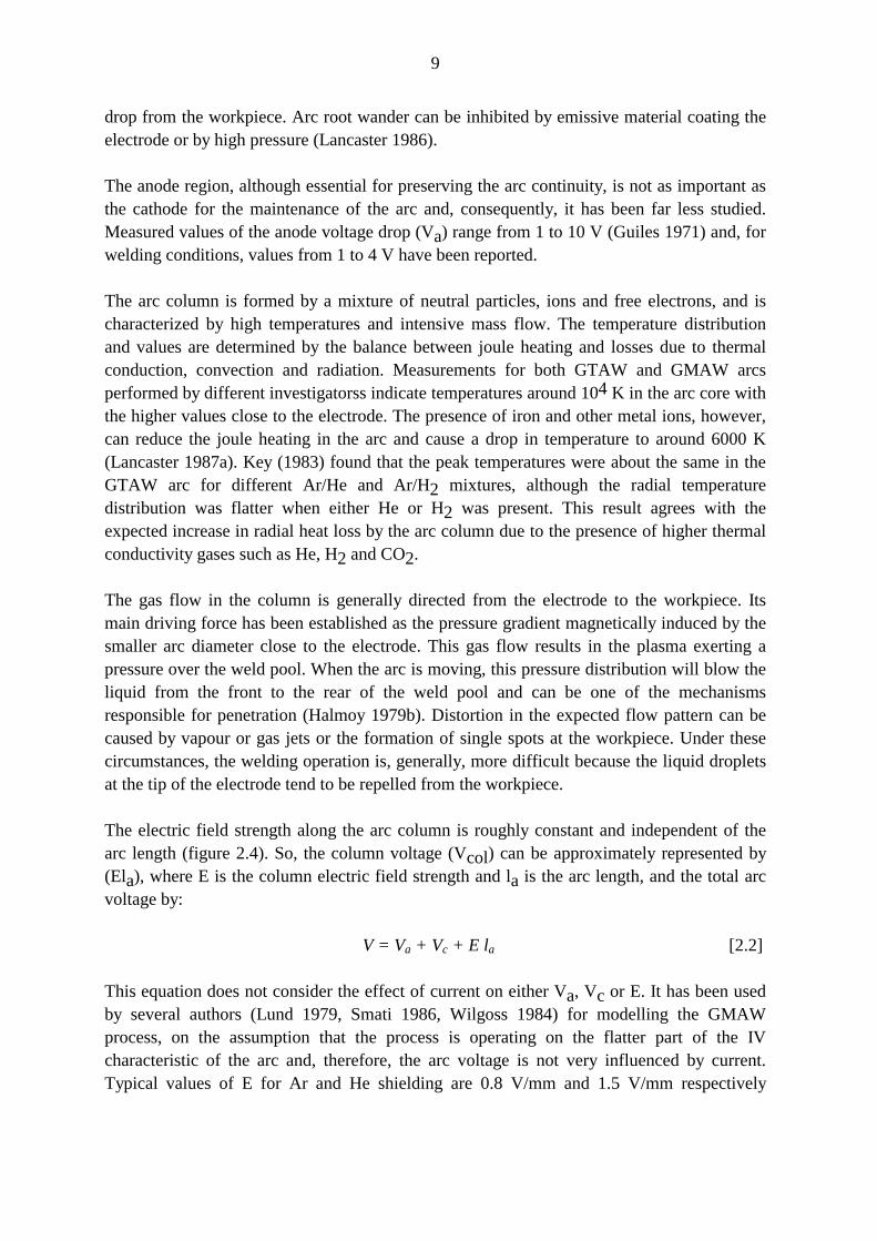
The electric field strength along the arc column is roughly constant and independent of thearc length (figure 2.4). So, the column voltage (Vcol) can be approximately represented by(Ela), where E is the column electric field strength and la is the arc length, and the total arcvoltage by:
V = Va + Vc + E la [2.2]
This equation does not consider the effect of current on either Va, Vc or E. It has been usedby several authors (Lund 1979, Smati 1986, Wilgoss 1984) for modelling the GMAWprocess, on the assumption that the process is operating on the flatter part of the IVcharacteristic of the arc and, therefore, the arc voltage is not very influenced by current.Typical values of E for Ar and He shielding are 0.8 V/mm and 1.5 V/mm respectively
10
(Allum 1986). A different equation which considers the rising part of the arc characteristicwas employed by Oshida et al.(1982):
V = α la + β + (γ la + δ) I [2.3]
where α, β, γ and δ are constants characterizing the arc. Finally, Ayrton's equation developedin the beginning of the century for low current carbon arcs is still commonly used inrepresenting the overall arc characteristic curve:
V = a + b la + (c + d la) / I [2.4]
2.2.3.Metal Transfer
The way in which the molten metal is transferred from the electrode tip to the weld poolaffects spatter and fume levels, positional capabilities, bead characteristics, and processstability and performance. The study of metal transfer has been of interest since consumablearc welding was introduced. The work in this area, done up to the early forties and relatedmainly to manual metal arc welding, was reviewed by Spraragen and Lengyel (1943). Afterthe development of the GMAW process, most of the investigations shifted to the new processpartially because of its ideal characteristics for studying metal transfer. During the late fiftiesand early sixties, the phenomena of metal transfer and its governing mechanism receivedconsiderable attention (see, for instance, Cooksey and Milner 1962, Amson and Salter 1962,and Smith 1962). In the seventies and eighties, the area of study has changed to include theeffect of arc current pulsing on metal transfer, flux cored wires, plasma-MIG welding and thedevelopment of theoretical models. A practical review on the subject has been recentlypresented by Norrish and Richardson (1988) and more fundamental ones by Lancaster (1986,1987b).
There have been several attempts to classify, on a phenomenological basis, the numeroustransfer modes observed in welding. Unfortunately, the many facets of metal transfertogether with the overlapping and, sometimes, confusing terminology, make it difficult topresent a standard classification for metal transfer modes (Killing 1984). The classificationsystem developed by the International Institute of Welding is reproduced in table 2.1. Someof the transfer modes more relevant to GMAW are briefly described in table 2.2 andillustrated in figure 2.5.
The transfer mode is determined by several factors, such as, welding current and voltage,polarity, wire diameter and material, shielding gas composition, arc length and electrodestickout.
A simplified representation of the relationship between welding current and voltage, andmetal transfer mode is shown in figure 2.6. In the welding of some metals (includingaluminum and steel) with electrode positive and argon based shielding, a well defined current
11
level above which the transfer mode changes from globular to spray (transition current, lineA-A' in figure 2.5) is observed. Lesnewich (1958b) performed an extensive study of theeffect of several factors on the transition current. Chilung et al. (1982) associated thetransition current with alterations in the arc root in the electrode and showed that oxygenadditions to argon first decrease and, when more than 5% O2 is present in the shieldingmixture, increase the transition current. CO2 additions to argon based shielding alwaysincrease the transition current.
Odd arc instabilities and disordered metal transfer have been observed under spray-transferconditions, and ascribed to variations in material composition (Hutt and Lucas 1982). Stronggas or vapour evolution and droplet explosions were observed with the aid of high speedcinematography for both aluminum alloys (Woods 1980) and steel (Lucas and Amin 1975).Rodwell (1985) observed arc instabilities and changes in metal transfer, weld bead profileand wire melting rate when welding with mild and stainless steel wires. These conditionswere attributed to the composition or surface condition of the wire, rather than to any featureof the welding technique.
Spray transfer is not commonly observed in negative electrode GMAW because reactionforces created by the cathode spots on the wire surface prevent the metal drops fromdetaching. However, spray transfer can be induced by wire activation (Lesnewich 1958a), byhigher ambient pressure (Nishiguchi and Matsunawa 1976), or by running the arc inside anarrow gap or groove (Ono et al. 1981).
Several models have been proposed for the qualitative and quantitative interpretation ofmetal transfer. Most of these models are based on the supposition that several different forcesact in the molten metal at the wire tip, and that the transfer process is governed by the staticbalance of these forces. Some of the forces that can participate in metal transfer are (Norrishand Richardson 1988):
- Gravitational force.- Gas flow induced force.- Electric magnetic forces.- Vapour/gas jet forces.- Surface tension.
General expressions for these forces were reviewed by Jilong Ma (1982) and Norrish andRichardson (1988). Jilong Ma (1982) also reviewed the models for metal transfer based onthe balance of forces assumption. A different modelling approach for metal transfer, based onthe instability of a current-carrying cylinder, has been adopted by Lancaster (1979) andextended by Allum (1985a). These models are far more complicated than static models andhave had a limited use so far.
Pulsed GMA welding was introduced to extend spray-type transfer to current ranges belowthe spray transition current where metal transfer is generally less controllable. It is based onthe use of a low background current to pre-melt the wire tip in combination with a peak
12
current above the transition current level to detach the molten material as a small droplet(Needham and Carter 1965). If the peak duration is too long or its intensity is too high, anumber of drops transfer, generally by stream spray transfer, during one peak period. Lowpeak current or short peak duration results in one drop transferring over several peaks. Acondition of one pulse-one drop transfer can be achieved by a proper selection of peakintensity and duration, and better transfer characteristics are obtained under this condition(Jilong Ma 1982, Maruo and Hirata 1982).
Several authors have determined conditions for one pulse-one drop transfer for different wirecompositions and diameters, and different shielding gases (Matsuda et al. 1983, Ueguri et al.1984, 1985, Amin 1983, Trindade and Allum 1984, Smati 1986, Foote 1986 and OliveiraSantos 1986). In most of these studies the conditions for one pulse-one drop transfer could berelated to peak current and duration by a simple empirical relationship:
Ipn tp
n = D [2.5]
where D is the detachment parameter and n has a value close to 2. Using the instabilitytheory and a simplified pulse structure, Allum (1985a) found n = 1.556. The conditions forone pulse-one drop transfer found by different authors for 1.2 mild steel wire are showntogether in figure 2.7. The results generally agree rather well considering the differentexperimental conditions that were used.
2.2.4.Wire Melting Rate
It is generally accepted that the wire melting rate in GMA welding can be calculated from theenergy balance at the wire tip (Lancaster 1986):
Qout = Qin [2.6]
Qout is the power necessary to heat a wire being fed at a speed w, up to its melting point,fuse it, overheat the molten metal up to its temperature just before detachment, and, finally,vaporize a fraction of the molten metal. This can be summarized by the equation below:
Qout = σwAw[Hm + (Td - Tm)cp + fvHv] [2.7]
where σ is the wire density,w is its melting rate,Aw is the wire cross section,Hm is the energy for wire heating and fusion,Tm is the material's melting point,cp is the material's thermal capacity,Td is the molten metal temperature just before its detachment from the wire tip,fv is the fraction of material vaporized, and
13
Hv is the material's latent heat of vaporization.
Assigning a value to Qout can be difficult because of the uncertainties related withexperimental measurement of Td and fv and the effect of welding parameters on them.According to Lancaster (1987b), results from different authors suggest, for steel wires,temperatures well above 2000°C. However Halmoy (1979) has found evidences oftemperatures close to the melting point.
Several factors, such as joule heating of the wire, heating generated at the anode (electrodepositive) or the cathode (electrode negative), radiation and convection from the arc column,radiation from the weld pool, heat generated by chemical reactions at the drop, etc, can becandidates to contribute to the formation of Qin. However, it is well established in theliterature that most of Qin is made up of the two first factors (Lesnewich 1958a, Lancaster1986):
Qin = Qjoule + Qa (for DC+) [2.8]
The anode heating (Qa) is generated by electrons entering the anode from the arc. It isformed by the thermal energy of the electrons ((3/2)kTI/e), the kinetic energy they receivecrossing the anodic fall (VaI) and the energy they release being absorbed by the metalstructure (φ I):
Qa = [(3/2)kT/e + φ + Va ].I [2.9a]
If the terms inside the brackets are considered constant, the anode heating will beproportional to the welding current:
Qa = k1.I [2.9b]
When welding with electrode negative, Qa should be replaced by the cathode heating (Qc)(Lancaster 1986):
Qc = [Vc - (φ + (3/2)kT/e)].I [2.9c]
Where Vc is the cathode fall voltage.
The importance of joule heating for wire melting was recognized by Wilson et al. (1956).This heating term cannot be calculated directly because the temperature of the wire in thestickout changes from room temperature, close to the contact tip, up to the material's meltingor boiling point in the arc root, and, consequently, electrical resistivity is not constant alongthe stickout. The temperature distribution and voltage drop in the electrode stickout havebeen theoretically calculated by Villeminot (1967), Amson (1972), Waszink and Heuvel(1979), Halmoy (1979) and Wilgoss (1984). Waszink and Heuvel (1979) also measured thevoltage drop along the stickout using a tungsten probe. Villeminot (1967), Lund (1979),
14
Waszink and Heuvel (1979) and Halmoy (1979) concluded that the electrical resistivity ofthe wire stickout can be considered approximately independent of welding current and,therefore, the joule heating term can be represented as:
Qjoule = k2.s.I2/Aw [2.10]
where k2 is a constant, and s is the stickout. Using equations [2.6] to [2.10] it can be shownthat, for electrode positive:
w = (k1I + k2sI2/Aw)/σAw[Hm + (Td - Tm)cp + fvHv] [2.11a]
or
w = α.I + ß.s.I2 [2.11b]
and
α = k1/σAw[Hm + (Td - Tm)cp + fv.Hv] [2.12a]
β = k2/σAw2[Hm + (Td - Tm)cp + fv.Hv] [2.12b]
Similar equations can be developed for electrode negative.
Quintino (1986) and Oliveira Santos (1986), working with mild and stainless steels,suggested that the α and ß coefficients are roughly proportional to the inverse of Aw and ofAw squared, respectively, as expected from equations [2.12a] and [2.12b]. Lesnewich(1958a) obtained similar empirical relationships but with a different power of Aw.
Equation [2.11b] was first proposed by Lesnewich (1958a) and, later, by Halmoy (1979).This expression is the most accepted in the literature and has been extensively used inmodelling the GMAW process (Lund 1979, Smati 1986), process control (Fujimura et al.1988), and extended to pulsed welding (Quintino and Allum 1984, Smati 1986, Foote 1986).Different equations based on regression analysis of experimental data have been proposed byThorn et al. (1982) and Chandel (1988). Chandel's equations included a VI and a constantterm in addition to the terms of equation [2.11b]. However, he used in his model the standoffdistance instead of the electrode stickout. Therefore, his s term included also the arc lengthand was sensitive to changes in voltage. Thorn obtained, for experiments with constantstickout, a simple linear relationship between current and melting rate and argued that theinclusion of a I2 term did not contribute significantly to the model. However, his results canalso be described well by equation [2.11b], even when coefficients from other authors areused.
The ß coefficient represents the mean resistivity of the electrode stickout and depends on theelectrode composition. It is negligible for high conductivity metals such as aluminum but can
15
have considerable importance for steel wires and its value depends on steel composition(Foote 1986). The joule heating of the electrode tends to be higher in pulsed GMAW than innon-pulsed welding. This can be shown by integrating equation [2.11b] over a pulse period(Quintino and Allum 1984, Smati 1986):
w = αImean + ßsIeff2 [2.13a]
or (Richardson and Nixon 1985), assuming a square shaped pulse current:
w = wnp + ßs(Ip - Ib)2tptb/(tp + tb)2 [2.13b]
Where Imean is mean welding current, Ieff is effective current, wnp is the melting rate fornon-pulsed welding with I = Imean, t is time and the subscripts p and b refer respectively topeak and base levels. As effective current increases, for the same mean current, when peakcurrent is increased, the wire melting rate should also increase as confirmed by differentauthors (see, for instance, Takeuchi 1984, Allum 1983).
The anodic heating coefficient (positive electrode welding) depends mainly on the electrodecomposition (Lancaster 1986). Several studies have shown it to be roughly independent ofthe welding current, shielding gas composition (Lesnewich 1958a, Quintino and Allum 1984,Ono et al. 1981), arc length and voltage (Lesnewich 1958a, Nunes 1982), electrode surfacecondition, joint gap width (Matumoto et al. 1980) and pressure.
Kyohara et al. (1977 and 1979) observed an increase in the melting rate of aluminum alloyswhen the arc length was less than 8mm and explained such behaviour by changes in anodicheating and droplet temperature due to alterations in arc shape. Similar results were found byTrindade (1984). Kinks or "discontinuities" in the melting rate when plotted against currentwere found by Nunes (1982) and Jilong Ma and Apps (1982). These irregularities were closeto the spray transition and were also associated with changes in anode heating and droplettemperature.
The cathodic melting coefficient is generally higher than the anodic coefficient in GMAW.The difference varies from around 75% in aluminum to 30% in copper (Lancaster 1986). Thecathodic melting coefficient is significantly affected by current level, electrode surfacecondition (Lesnewich 1958a), shielding gas composition (Yamauchi and Jackson 1976, Ono1981), joint gap width (Matumoto 1980), arc length and pressure. The cathode burnoff canbecome lower than the anodic burnoff under the influence of electrode surface treatments orhigh pressure (Lancaster 1987).
2.2.5.Shielding Gases
The primary reason for using any sort of shielding medium in welding is to protect the arc,wire tip, molten pool and surrounding base material from atmospheric contamination.
16
Furthermore, many other factors, such as metal transfer mode, spatter and fume generation,weld bead geometry and composition, etc are affected by shielding gas composition.
Some of the first attempts to weld with consumable electrodes under both inert and activegas protection were performed by Doan and co-workers (1938, 1940) who alreadyrecognized, at that time, the greater difficulty in welding mild steel with pure inert gas. Whenthe process was commercially introduced in the forties for welding aluminium alloys, onlypure argon and helium were used for shielding. Eventually, mixtures containing oxygen weredeveloped for stainless and mild steel. In the mid fifties, carbon dioxide was introduced as acheaper alternative for mild steel welding. Since then, different Ar-O2-CO2 mixtures havebeen developed commercially for the welding of steel in an effort to obtain the best balanceamongst the many conflicting factors that are influenced by gas shielding. The same basicmixtures have been used for pulsed GMAW. Quintino and Allum (1984), and Cuny (1988)recommend mixtures containing >90% Ar, plus oxygen and carbon dioxide, for pulsedGMAW of mild and low alloy steels. The selection and basic characteristics of shieldinggases and mixtures have been revised many times since the introduction of gas shieldedprocesses: Helmbrecht and Oyler (1957), Salter and Dye (1971), Cresswell (1972), Brosilow(1978), Weld. Design & Fab. (1988), Hilton and Norrish (1988), for instance. Table 2.3summarises the gas mixtures available and their applications. This section will be concludedby a discussion about the influence of additions of He on the argon shielded welding arc.
In GTAW, the argon arc is bell-shaped and whitish-grey (Hiraoka et al. 1986) and has anelectric field strength of approximately 0.7-0.9 V/mm. When helium is gradually added tothe shielding, the arc is altered by a progressive change to a spherical light-green form. At thesame time, arc voltage increases (Helmbrecht and Oyler 1957, Hiraoka et al. 1986) while arcpressure and radial temperature gradient decrease. Its electric field strength, however,remains approximately constant up to 75% He and then increases sharply to around 1.3-2.0V/mm (Ludwig 1959, Hiraoka et al. 1986). When welding aluminum with alternatingcurrent, the use of helium results in poor arc stability and poor cleaning action (Helmbrechtand Oyler 1957). Such changes in arc behaviour have been ascribed to the difference inphysical properties of the two gases, namely, their ionization potential and thermalconductivity (table 2.4). However, a clear mechanism for such differences is not yetavailable.
Trends similar to those described above are present in GMAW. Moreover, helium additionstend to make it more difficult to obtain spray transfer and, above 80% He, only globulartransfer and a consequent loss in arc stability are obtained (Kennedy 1970). When studyingthe arc shape and metal transfer for different shielding gases, Hazlett and Gordon (1957)observed that, in helium shielded welding, the arc was mainly confined to the region betweenthe bottom of the drop and the workpiece. Periodically the arc seemed to extend up the wire.When argon was used for shielding, the metal transferred mainly by spray but somedisturbances in metal transfer were also observed. In pulsed welding, Hilton and Norrish(1988) suggested a limit of 85% He above which the process stability deteriorates.

17
Studies of the effectiveness of shielding gas cover using Schlieren techniques (Cunninghamand Cook, 1953) indicate that, due to its lower density (table 2.4), helium requires a flow twoto three times that of argon for equivalent shielding. As a rule of thumb, Hilton and Norrish(1988) suggested that adequate shielding will be obtained with helium containing mixtures,by using an argon flowmeter and setting the flow reading to that of an argon/carbon dioxidemixture.
The total bead area is increased by additions of helium and other gases that increase the arcvoltage (at a fixed current). The bead width and the secondary penetration tend to increasewith the helium content while the finger penetration is less affected in aluminum GMAwelding (Kennedy 1970).
2.2.6.Equipment and Process Control
The primary equipment for GMA welding comprises a power supply, a wire feeder, weldingcables, a welding gun, flowmeter, regulator and hose for shielding gas supply, and,optionally, a water cooling system. Basic information concerning this equipment can befound elsewhere (Houldcroft and John 1988). Only a brief introduction on power suppliesand control in conventional GMAW and a review of some recent advances will be presentedhere.
2.2.6.1.Power Supplies
With regard to the electrical design and operative principle, the most widely used powersupplies for GMA welding can be broadly categorized into the following groups (Kolasa etal. 1985):
(1) Conventional transformer-rectifiers with magnetic flux control,(2) Solid state AC phase controlled rectifiers (thyristor control),(3) DC controlled power transistors (transistor series regulator and secondary chopper powersupplies), and(4) Primary inverters.
Conventional transformer-rectifiers rely mainly on mechanical or electrical systems foroutput adjustment and have changed little since the introduction of GMAW. The operationalprinciples and construction of conventional power supplies have been thoroughly discussedby Manz (1973).
The common feature of the latter three groups is the use of semiconductor devices for directcontrol of output current and/or voltage. When compared with conventional power supplies,the electronic based ones are characterized by (Yamamoto 1984, IIW Commission XII 1982):
18
- Higher performance: Dynamic response and reproducibility far superior toconventional power supplies.
- Multiple functions: The possibility of controlling the output by a small currentand the use of feedback control allowed the development of power supplies withmultiple VI characteristics.
- Easier connection with peripheral equipment and programmability: The use ofelectronic circuitry allows the power supply to receive input signals from sensors,internal microprocessors, external computers, etc. Pre-programmed "optimal"welding conditions or a set of pre-established rules (logic) for parameter selectioncan be stored in electronic memory and used to define the power supplyoperation. Such capability permitted the development of power supplies that canbe prepared for operation through a single switch, the so-called "one-knob"machines.
- Reduction of weight and cost: The introduction in the 1980's of inverter typepower supplies have resulted in massive reduction in transformer size due to itsuse of high frequency alternating current. Consequently, the weight, size and costof electronic power supplies has decreased appreciably.
In spite of their increasing popularity and decreasing price, electronic power supplies are stillmuch more expensive than conventional ones. Their more complicated design is anotherlimitation. Basic constitutive aspects and characteristics of the different power supply typeshave been revised by the IIW Commission XII (1982), Kolasa et al. (1985), Norrish (1985)and Bréat (1987).
2.2.6.2.Control aspects in GMAW
Conventional GMAW operates with a power supply with a constant voltage (CV)characteristic and a constant wire feed speed which is generally set at the wire feeder. Underthese conditions, voltage (and consequently arc length) and wire speed remain approximatelyunchanged during welding while current and electrode stickout values result from those andthe standoff distance. Any perturbations in welding conditions (for instance, variations instandoff distance by the welder) are mainly absorbed by changes in current and stickout. Thecapability of keeping the arc length relatively constant (self-adjusting arc) is one of the mainreasons for the high popularity of constant-voltage equipment in GMAW until today (Weld.Metal & Fab. 1988). Another advantage of a CV system is ease of arc ignition due to therapid increase in current in the instant the electrode touches the workpiece.
In dip transfer welding, too fast an increase in current during the short circuit can lead to anexplosive rupture of the liquid bridge between the wire and the weld pool, which results inspatter. Conventionally the current rise rate has been controlled by either sloping the VIcharacteristic or regulating the dynamic response of the power supply.
19
One problem with CV operation is that the system achieves equilibrium through variations incurrent which is one of the most important variables affecting formation of the weld bead. Inpulsed GMAW, metal transfer stability depends strongly on the pulse current and duration.The use of conventional CV power supplies with voltage pulses when pulsed GMAW wasfirst introduced made it difficult to determine favourable conditions for stable metal transfer(Nixon and Norrish 1988). Pulsed GMAW welding is often performed under CCcharacteristics nowadays although some alternative systems do exist (see below).
The development of electronically controlled power supplies in recent years brought about arevolution in terms of control methods (Allum et al. 1985). It has been particularly importantfor pulsed transfer where the selection of welding parameters is complicated by the need forspecifying the pulse structure for stable transfer. Some of the control techniques proposed forGMAW welding are described below:
. Synergic MIG: This term embraces a group of control techniques in which thecurrent structure is determined by the wire feed rate or vice-versa. Generally, atachogenerator signal from the wire feed system provides a control signal for thepower supply. The idea was originally developed in the Welding Institute for one-knob pulsed GMAW but the concept has also been applied to short-circuittransfer (Norrish 1988). The relationship between power supply output and wirespeed is determined by a set of rules called synergic algorithms (Quintino 1986).Several algorithms have been presented in the literature for both pulsed (Amin1981, Allum 1983) and short-circuit transfer (Amin 1986b). Synergic MIGcontrol has been achieving an increasing acceptance over the last few years and ithas been considered for use, together with real time seam tracking, in futureadaptive control systems for production welding (NMAB 1987).
. Voltage/arc length control: An alternative approach to synergic MIG has beensuggested in which a control signal from the arc voltage is used to drive thepower supply output (Ditschun et al. 1985, Essers and van Gompel 1984, Allum1985b). This type of control system mimics, by different mechanisms, the self-adjusting arc of CV systems and, therefore, suffers from similar limitations.
. CVCC operation: This technique has been implemented to improve arc self-adjustment in pulsed GMA welding without disturbing metal transfer (Nixon andNorrish 1988). It uses a constant voltage characteristic during the pulse phase anda constant current characteristic in the background period. By using high peakcurrents of short duration the system operates in a region in which the one pulse-one drop transfer is not sensitive to peak current (see figure 2.7).
. Adaptive control: This technique involves feedback plus allowance forinteraction between varying factors (i.e., arc length, travel speed, torchorientation, wire feed speed, track guidance, fusion control, joint fill, defect
20
formation, etc) measured, fed back, and compared with original set points andthen perhaps modified by a complex interpretation of the process dynamics(Emerson 1988). A few systems have been suggested in which real timemonitoring is used to control welding conditions and joint tracking, and performany necessary correction. Different monitoring techniques have been proposedsuch as through-the-arc monitoring (Thompson 1986, Nomura et al. 1986),inductive sensoring (Blume et al. 1988) and weld pool imaging (Oshima 1988).
The recent advances in welding power supplies and process control have revolutionized theapplication of the GMAW process. However, they have not been able to solve one of themajor limitations of the process, namely the likelihood of fusion problems. A more profoundunderstanding of the basic mechanisms in GMAW in conjunction with the tightercontrollability available nowadays can be a possible approach to alleviate such problems.
2.3.NARROW GAP WELDING
2.3.1.Introduction
Although narrow gap welding (NGW) has generated great interest in the welding industryand has been the subject of much investigation in the last twenty years, there is still somecontroversy around a proper definition for the technique. Most authors agree that narrow gapwelding is performed in thick joints using an essentially square butt joint preparation withsmall gaps (Henderson 1978, Baxter 1979, Nazarchuk and Sterenbogen 1984). Bicknell andPatchett (1985) suggested that a joint aspect ratio (plate thickness to gap width) of 5 or moredefined a welding process as "narrow gap". Electro-slag welding and even electron beamwelding have been included as narrow gap processes by some authors, whereas others haverestricted the term to arc welding only. In an attempt to systematize the concept of narrowgap welding, Malin (1983, 1987) distinguished the following features of NGW:
- NGW is not a welding process, it is a special bead deposition technique,- NGW is associated only with an arc welding process, for instance, gas metal arc
welding (GMAW-NG) or submerged arc welding (SAW-NG),- NGW features a fixed bead deposition layout that is characterized by a constant
number of beads per layer (1-3) deposited one on top of the other,- NGW requires a square groove only. When a groove angle is used, it is intended
for distortion compensation rather than for better access to the joint. When used,the groove angle is generally around 2-3 degrees only.
- NGW requires low or medium heat input.
and, based on those features, defined narrow gap welding as:
21
"NGW is a property-oriented bead-deposition technique associated with an arcwelding process characterized by a constant number of beads per layer that aredeposited one on top of the other in a deep, narrow square groove."
A very similar definition is given by Manzoli and Caccia (1989).
The development of NGW was intended to reduce weld metal volume in thick plate weldingand hence reducing welding cost, time and distortion level. The technique was first describedin the USSR (Dudko et al. 1957) and in the United States (Meister and Martin 1966), and itwas developed and used mainly in Japan, where several different approaches have beenproposed in order to overcome its limitations. A classification of the NGW processescommonly used in Japan is shown in figure 2.8 (Nomura and Sugitani 1984). A more recentand comprehensive classification is given by Malin (1987), figure 2.9. This classification isbased on the criteria below:
- Welding processes associated with NGW.- NGW technique, including electrode feeding technique, bead deposition layout
and number of electrodes used simultaneously.
The main welding processes associated with NGW are gas metal arc welding, submerged arcwelding (SAW), gas tungsten arc welding (GTAW) and flux cored arc welding (FCAW).According to Lucas (1984), NGW is basically applied to GMAW (78%), SAW (18%) andGTAW (4%) in Japan. In the western countries, NGW is much less common and more usedwith SAW (Malin 1987, Lucas 1984, Bicknell and Patchett 1985). Recent developments infiller metal and flux formulation, and the greater tolerance of SAW-NG to welding parametervariation (when compared with GMAW-NG) have increased the interest in narrow gaptechniques based on SAW (Malin 1989). However such applications are basically confined tothe flat position.
NGW processes can be separated into two groups based on the electrode feeding techniqueused to ensure adequate sidewall penetration. The first group (NGW-I) achieves sidewallpenetration through electrode/arc manipulation, including directing fixed electrodes towardsthe sidewall (NGW-Ia), oscillating (NGW-Ib) or rotating (NGW-Ic) the arc. The secondgroup (NGW-II) attempts to control sidewall penetration through manipulation of weldingparameters (Malin 1987).
NGW is more frequently performed with one or two passes per layer (monopass or bi-passdeposition layouts). A tri-pass layout is less common. Finally, according to the electrodearrangement, NGW torches can be single or double-electrode.
Some of the advantages attributed to NGW processes, when compared with other weldingprocesses for thick joints, are listed below:
- reduction in welding time,
22
- lower consumable costs,- reduction in slag removal time,- reduction in preparation cost,- reduction in post-weld heat treatment,- improved toughness, and- reduction in angular distortion.
These advantages, which are directly related to the lower weld metal volume and heat inputof NGW, are expected to result in lower costs for welding thick material when comparedwith conventional processes such as SAW and ESW (figure 2.10).
The main problems with narrow gap techniques are associated with the high sensitivity ofNGW to the formation of defects such as lack of fusion, undercutting and centre linecracking as a result of minor variations in welding conditions. Pore formation due toimproper gas shielding and magnetic arc blow are also frequent problems associated withGMAW-NG, whereas entrapped slag can occur in SAW-NG. These problems, together withthe difficulty in repairing welding defects in thick joints, have led to the development ofcomplicated and expensive welding equipment for NGW (Malin 1987) that requires a veryexperienced and well trained operator in order to achieve reliable operation (Hunt 1985).Results obtained with the industrial implementation of both GMAW-NG and SAW-NGsuggested that the likelihood of defect formation in the former was higher than in the latter(Hunt 1985).
Several reviews of narrow gap welding have been published since its introduction in thesixties, for instance, Henderson (1978), Baxter (1979), Malin (1983 and 1987) and Ellis(1988).
2.3.2.Narrow gap GMAW
Gas metal arc welding was the first process to be used in NGW and it is still the one mostcommonly associated with the technique. This preference is related to the easily observablearc, relatively narrow groove, high welding quality, productivity and cost effectiveness(Malin 1987). However, GMAW-NG is rather prone to defect formation in the sidewalls,spattering and shielding gas deficiencies. These problems, which are associated with thedifficulty in feeding the electrode and supplying a proper shielding gas coverage into a verynarrow and deep groove, and in obtaining well balanced arc heating between the side wallsand the bottom of the joint, have been the major obstacles to a greater acceptance of GMAW-NG. In order to overcome these limitations, several wire deposition strategies and torchdesigns have been proposed, developed and some of them used in industrial applicationssince the introduction of narrow gap welding.
NGW-I techniques for GMAW have been developed mainly in Japan and comprise severalprocess variations including:
23
- Pre-casting the wire and depositing alternating stringer beads (Meister and Martin1966), NGW-Ia.
- Oscillating the wire inside the groove using a straight long contact tube that isswung across or along the groove (Nakayama et al. 1976, Futamura et al. 1978),NGW-Ib.
- Rotating alternately a bent contact tip about its axis inside the groove (Innyi et al.1975), NGW-Ib.
- Plastically deforming the wire into some wavy shape before its entrance in thecontact tube in order to oscillate the arc across the groove (Sawada et al. 1979,Probst and Hartung 1988), NGW-Ib.
- Rotating the arc by feeding the wire through an eccentric contact tube that rotates(Nomura and Sugitani 1984), NGW-Ic.
- Rotating the arc by using a special "twist" electrode wire (Kimura et al. 1979),NGW-Ic.
Thin wires (less than 2.0mm) are typically employed with NGW-I techniques. This isexplained by the necessity of bending or plastically deforming the wire in almost all theprocesses. One exception is the twist wire technique that employs two 2.0mm interwinedwires with an equivalent diameter of 2.8mm. The heat input in some of the processes is lowenough to allow their use in positional welding. Gap width depends on the specific techniqueemployed and wire diameter, and values between 6mm and 20mm have been reported in theliterature. Mechanical wear of contact tube and other parts, fluctuations in the current pick-uppoint and inconsistencies in wire feeding are potential problems associated with most ofNGW-I processes (Render 1984, Allum and Foote 1984). Making the arc oscillate across thejoint, however, has the positive effect of increasing the process tolerance to groove widthvariations, reducing side wall defects and, consequently, enlarging the process operationalenvelope when compared with NGW-II techniques.
The main general characteristics of NGW-II techniques are the following (Malin 1987): arelatively large electrode diameter is used, ranging from 1.6mm to 5mm, a long electrodestickout is maintained in the centre of the groove with the contact tip located out of the jointgap, the heat input and the deposition rate are higher, and the gap opening is generally wider(11-16mm) than those employed in NGW-I. The high heat input generally limits use to theflat position only. Overheating and softening of the electrode wire by joule effect heatinglimit the maximum thickness (around 150mm) that can be welded to a much lower valuethan that achieved by NGW-I techniques. The equipment for NGW-II is basically the same asthat used in conventional GMAW apart from slight modifications. Sidewall penetration iscontrolled by careful selection of welding parameters, including electrode polarity and
24
shielding gas composition (Kurokawa et al. 1966, Jackson and Sargent 1967, Lebedev 1977).A different approach for NGW-II has been recently considered by Fennel (1986) who, basedon an earlier analysis of Allum and Foote (1984), used relatively thinner wires (1.2mm),narrower gaps (around 7mm) and pulsed current for high speed horizontal welding ofpipelines in the horizontal-vertical position.
A comprehensive review of most of the GMAW-NG processes was presented by Malin(1987) and a summary of Japanese NGW techniques can be found in a paper by Jones(1984).
Argon plus 10-25% CO2 is the most commonly used shielding gas mixture for welding mildand low alloy steel with NGW. Mixtures containing higher levels of CO2 (Belchuk and Titov1970, Kurokawa et al. 1966, Jackson and Sargent 1967), Ar-5%CO2 (Matsunawa andNishiguchi 1979), Ar-5%CO2-2%O2 (Fennel 1986) and ternary mixtures containing Ar, Heand CO2 (Jackson and Sargent 1967, Lebedev 1977, Fennel 1986) have also beenconsidered. Carbon dioxide additions to argon affect both arc stability and bead shape. Ar-10%CO2 is considered the most acceptable mixture in terms of arc stability in NGW (Malin1987). Working with the "twist" wire process, Kimura et al. (1979b) found a maximum ofpenetration depth at the bottom of the joint for around 10%CO2, and a steady growth insidewall penetration with the CO2 content (up to 40%) in the mixture. A similarimprovement on sidewall penetration is associated with the helium content in the mixture,specially when it is more than 50%. However, helium additions also impair the processstability, particularly when helium content is over 75% (Lebedev 1977). Working withNGW-II, thin wires and pulsed current, Fennel (1986) also observed an improved lateralfusion when a helium based commercial mixture (Helishield 1, Ar-85%He-1.5%CO2-250Vmp O2) was compared with an argon based mixture (Argoshield 5, Ar-5%CO2-up to2%O2).
A major difficulty in GMAW-NG is to ensure an effective shielding gas coverage for the arcand weld pool inside the gap. The geometric configuration of the joint can promote air beingentrained by the shielding gas column inside the groove while the relatively long distancethat sometimes separates the gas nozzles from the arc, renders the process very sensitive todraughts (Kender 1984). As a result, porosity can be formed. A number of techniques havebeen proposed to improve the shielding conditions in GMAW-NG. The most commonly usedpractice is to increase simply the gas flow rate proportionally to the thickness of the joint(Probst and Hartung 1988). Using a NGW-II process, Kurokawa (1966) observed that, above100mm of joint thickness, the gas flow rate required to produce porosity free weld increasessharply from its initial value of 25 l/min (figure 2.11). Gas boxes seating directly over thejoint and fitted with protective shrouds to prevent air from being entrained, and flat nozzlesinserted into the joint to shield the arc area are generally used together for welding thickplates with the NGW-I technique.
Voltage, or perhaps arc length, is a key factor in providing adequate lateral penetration(Belchuk and Titov 1970, Kurosawa et all. 1966, Baxter 1979, Malin 1987) and process
25
stability (Lebedev 1977, Matsunawa and Nishiguchi 1979). When the arc voltage is too low,the side walls receive insufficient heat and lack of fusion is likely to develop. At the sametime, short circuiting conditions, spattering and an unstable arc can be observed. Increasingarc voltage improves lateral fusion but, if the arc length becomes too long relative to the gapwidth, the arc tends to jump to the side walls. Undercutting, slag entrapment and lack offusion at the bottom of the joint are then likely to develop. Under high voltage conditions andin a very narrow I groove, the arc can climb up rapidly along the side walls and render theprocess inoperative. Matsunawa and Nishiguchi (1979) associated such behaviour with thedistribution of cathode spots on the joint and reduced the problem by increasing the CO2content in the shielding gas. The effect of voltage on bead formation and process stability issummarised in figure 2.12.
Current affects deposition rates, arc stability and bead geometry. Penetration at the bottom ofthe joint and deposition rate increase when the current rises whereas lateral penetration is lessaffected in both NGW-I (Kurokawa 1966, Belchuk and Titov 1970) and NGW-II (Kimura etal. 1979). Therefore, height/width ratio and sensitivity to centre line cracking also tend toincrease. Current is generally kept above the spray transition level and pulsed current can beused to further stabilize the arc.
Unlike conventional GMA welding, which is performed almost exclusively with electrodepositive, most of the work related to NGW-II indicates a preference for electrode negative(Jackson and Sargent 1967, Kurokawa et al. 1966, Belchuk and Titov 1970, Lebedev 1977).The following beneficial aspects have been associated with welding with electrode negativeinside a narrow gap: higher productivity, greater sidewall penetration, lower height/widthratio and, therefore, lower sensitivity to centre line cracking. In electrode negative GMAW-NG, the confining walls of the groove affect the arc shape, resulting in an increase in arcstability, a change in metal transfer mode from repulsive globular to spray and a reduction inmelting rate, whereas in reverse polarity no significant alteration was observed (Matumoto etal. 1980). However, electrode negative GMAW-NG still presents arc stability problemsduring the final passes when the groove influence over the arc becomes unimportant.
Welding speed influences the tendency of the weld pool to flow under the arc, the lateralpenetration and the heat input. At low speed, the weld pool is likely to flow under the arc,preventing it reaching the lower corners of the groove and causing incomplete fusion(Kurokawa et al. 1966, Belchuk and Titov 1970). Increasing speed lowers the heat input inthe weld. However, excessive speeds can cause incomplete fusion into the sidewall, due toinsufficient heating of the wall (Malin 1987).
GMAW-NG is still the most used of the narrow gap processes. However, many problems,such as the tendency to lack of fusion, porosity and spatter generation, still remain basicallyunsolved. As a result, SAW has been increasingly used in narrow gap applications in thedownhand position. There are, however, positional welding situations, such as the J-layingwelding of pipelines, where neither SAW nor GMAW-NG with arc oscillation can beapplied.

26
2.4. MODELLING OF THE WELD BEAD SHAPE
2.4.1. Introduction
Modelling is an activity constantly performed by man in both scientific and non-scientificsituations. It involves creating an idealized representation of a real-world situation or systemto promote a better understanding of its behaviour, i. e., a model (Cross and Moscardini1985). A model, far from being an exact replica of the system, is a simplification of it andcontains only those elements or features that the modeller considered important and was ableto implement. At the same time, different approaches can be used for developing a model.Therefore, there is not a unique model for a system. Several different models can bedeveloped for a given system by considering different features of the system, by usingdifferent interpretations for the same features, or by considering different approaches formodel-building. Modelling is a fundamental tool for knowledge formation. However, amodel must never be confused with reality. Failure to distinguish model from reality hasfrequently happened and generally resulted in retarding the development of new ideas.
One the first steps in model-building is to clearly state the reason or objectives of the model.The objectives and the resources available (both material and intellectual) will greatlyinfluence the developing strategy, final form and applicability of the model. Cross andMoscardini (1985) suggested five main categories for models based on their objectives:
. system understanding,
. design,
. optimization with respect to prescribed constraints,
. control, and
. training.
Models can be classified in many ways. A classification system presented by Gordon (1978)first separated them into physical and mathematical models (figure 2.13).
Physical models are based on some analogy between such systems as mechanical andelectrical or electrical and hydraulic, or between the behaviour of different materials insimilar situations (for instance, plasticine has been used for studying the forming of metals,Awano and Danno 1972).
Mathematical models use symbolic notation and mathematical equations to represent thesystem. Both mathematical and physical models can be either static or dynamic according tothe influence of time on the model. Finally, Gordon classified mathematical models asanalytical or numerical based on the technique used to solve them. Mathematical models canbe further separated into theoretical or empirical, mechanistic or stochastic (statistical), and

27
discrete or continuous. Many other classifications for models are possible. It must beemphasized, however, that any classification system is rather artificial and should be usedonly as a reference. Models often present characteristics that do not allow them to be placedinto only one class.
2.4.2. Mathematical modelling
There is a strong motivation for modelling the formation of a weld bead. A weldingprocedure is specified by parameters such as welding current, voltage, speed, gascomposition, etc, but, as far as the weld applicability is concerned, the really importantfactors are the output variables (welding geometry, fusion characteristics, mechanicalproperties, etc). The inter-relationship between input and output variables in arc weldingprocesses is rather complex and is traditionally obtained by a trial-and-error approach, basedon previous experience and subjective judgement. This approach has, however, somedrawbacks. It is subject to human error; it is not of universal application; it contributes littleto the understanding of the problem and yields a solution which, while being acceptable, isnot necessarily optimum in terms of cost or quality (Galopin and Boridy 1986).
A considerable amount of work has being undertaken to model the relationship between weldbead shape and welding parameters. However, the large number of complex and interactingvariables and, until recently, the relatively poor precision and controllability of weldingequipment, particularly power supplies, have created some scepticism regarding the use ofmathematical models in procedure specification and process control. This trend seems to bereversing in the last 10 years. Several factors have contributed to this change, for instance:
. Computers have become cheaper and more powerful.
. The use of electronic power supplies and other modern welding equipment haveincreased the reproducibility and precision of welding, and made it possible todirectly inter-connect welding equipment, computer and sensing devices.
. There has been a trend to switch from manual and semi-automatic welding,where the welder subjectively adjusts welding parameters in order to control beadformation, to automatic welding, where the scope for such intervention is muchreduced and may never be considered.
The work related to mathematical modelling of weld bead geometry has been reviewed byShinoda and Doherty (1978), and McGlone (1982). In both papers the different models aredivided into two main categories: theoretical and empirical approaches. Although thiscriterion is rather artificial, it is as good as any other criterion used to organise the differenttrends for modelling the weld bead shape and will also be used in the present work.

28
2.4.2.1. Theoretical approach
Theoretical studies of the weld bead formation have been mainly based on the work byRosenthal (1946) who solved analytically the heat flow equation:
( ) ( ) ( ) sTkcTvcTt
+∇⋅∇=∇⋅+∂∂ rρρ [2.14]
where v is the welding velocity, k is the thermal conductivity of the workpiece, _ is the density, c is the specific heat, and s is the heat created or absorbed,
for welding conditions using the following assumptions:
. the physical characteristics of the metal are independent of the temperature andphysical state of the metal,
. quasi-equilibrium of thermal conditions,
. the heat source is reduced to either a point, a line or a plane,
. the workpiece has a very simple geometric shape in which one, two or all threedimensions are infinite.
For the case where a point heat source is moving on the surface of a very thick plate,Rosenthal's solution is:
( )
+−+= Rxv
kRqTT
απ 2exp
20 [2.15a]
for a linear heat source moving in a plate of thickness h the solution is:
−+=
ααπ 22exp
2 00vrKvx
kqTT [2.15b]
where T is the temperature at point (x,y,z), T0 is the plate initial temperature, α = k/σc is the thermal diffusivity, q = nVI is the arc effective heat input, R = (x2 + y2 + z2)1/2, r = (x2 + y2)1/2, and K0 is the modified Bessel function of zero order.
Rosenthal's model has been modified and extended by several workers. For instance, Wells(1952) simplified equation [2.15b] in order to obtain the bead width, Adams (1958)
29
calculated the peak temperature distribution in the workpiece, Cline and Anthony (1977)considered the effect of a gaussian heat source, and Nunes (1983) introduced the concept ofthermal dipoles to account for the heat liberated by phase transformations. The validity ofRosenthal's model was investigated by Christensen et al (1965) by transforming [2.15a] and[2.15b] into dimensionless equations and comparing the theoretical bead area, width andpenetration with a large number of experimental results. Moore et al. (1985) compared thecooling times from Rosenthal's model against the results of a finite elements model. It hasbeen shown that the model predicts adequately well temperatures and cooling rates at somedistance from the weld pool, and the cross-sectional areas of the fusion zone (autogenouswelding) and the heat affected zone, provided the welding speed is sufficiently slow (Kovityaet al 1986). Equation [2.14] has also been solved numerically by different authors in anattempt to reduce the simplifications necessary for an analytical solution, for instance, Ushioet all (1977), Kou and Lee (1983), Kovitya et al (1986), and Tekrival and Mazumder (1986).
Rosenthal's model and the work following his approach have ignored fluid flow in the weldpool completely. This flow can be an important factor in the formation of the weld bead,determining, for instance, the occurrence of finger type penetration in spray-GMA welding(Halmoy 1979b). It is also associated with cast-to-cast variations of penetration in GTAwelding (Heiper and Roper 1982). Convective motion is caused by electromagnetic,buoyancy and surface tension forces. In order to obtain the convective profile in the weldpool, the equation of continuity:
⋅∇ v = 0 [2.16]
the momentum equation:
BJgvnpvv ×++∇∇−−∇=∇⋅ σσ [2.17]
and thermal balance equation [2.14] have to be solved. Different boundary conditions may beconsidered (Szekely 1986):
. heat and current flux distribution in the free surface,
. latent heat to be supplied or released at the solid-liquid interface,
. surface tension value and gradient at the free surface,
. free surface profile,
Several solutions for this problem have recently been presented in the literature. Atthey(1980) studied convection due to electromagnetic forces in a hemispherical weld pool.Oreper and Szekely (1984) and Craine (1987) analyzed the formation of the weld pool instationary GTAW considering the effect of surface tension gradients on weld pool convectionand bead shape. Kou and Wang (1986) modelled continuous operation GTA welding.Finally, Zacharia et al. (1988 a,b) studied bead formation in both non-autogenous andautogenous GTA welding considering the influence of a non-planar free surface, and Tsao
30
and Wu (1988) modelled stationary GMA weld pool. Similar models were also proposed forelectron beam (Wei and Giedt 1985) and laser welding (Davis et al. 1986).
The static pressure balance of surface tension and gravity forces was used by Nishiguchi etal. (1975, 1977) to model the weld reinforcement profile in overlay and horizontal filletwelding. To simplify the model solution, the theoretical analysis is made under the followingassumptions:
. The weld pool is considered infinitely long in the direction of welding (twodimensional model),
. The digging action by the arc is negligibly small, and
. The surface tension is constant all over the pool surface.
For bead-on-plate welding, and taking the origin at the vertex of the bead (figure 2.14), thepressure balance is given by:
τ/R = τ/R0 - σgy, 1/R = y''/(1 + y'2)3/2 [2.18]
Where τ is the surface tension, 1/R0 is the curvature at origin, and 1/R is the curvature at point (x,y).
From equation [2.18] the weld surface profile can be derived as function of elliptic integrals.
A similar approach has been used by Andrews et al. (1980) to model both face and rootprofiles for the horizontal welding of thin plates, by Berezovskii et al. (1983) to study theface profile in horizontal welding, and by Richardson (1986) to analyze weld pool sagging innarrow-gap horizontal welding.
2.4.2.2.Empirical approach
Empirical modelling, often used together with simple theoretical ideas based on Rosenthal'smodel and applied to a specific situation, has been the most commonly adopted modellingtechnique employed to study the relationship between process variables and weld bead shape.Submerged arc welding has been the process most frequently associated with these studies.This preference can be explained by the relative facility with which the levels of the weldingparameters in this process can be made sufficiently distinct from one another to permit ageneral understanding of the relationship between input and output variables (McGlone1982). The majority of the analysis has been carried out on downhand, bead-on-platewelding. Shinoda and Doherty reviewed the empirical modelling work performed up to 1978.
Thorn et al. (1982) obtained simple regression models for the dimensions of GMA welds.These results were compared with values predicted by theoretical models obtained by Wells
31
(1952), and Christensen et al. (1965). The empirical model by Jackson and Shrubsall (1953)for penetration in SAW was also compared:
p = k.[I4/ (v.V2)] [2.19]
where k is a constant that depends on the welding process.
As expected, the regression models were considered the most appropriate to describe theexperimental data from which they were created.
Quintino (1986) studied the fusion characteristics of pulsed GMAW in mild steel plates and,based on Wells' model, related dilution to the factor Imeanv. The semi-empirical relationshipobtained was:
1/δ = 1/δmax + k/(Imean.v) [2.20]
where k is a constant, δ is dilution, and δmax is the maximum dilution.
and a chart for the generalised representation of fusion characteristics was prepared (figure2.15). A very similar approach was followed by Allum and Oliveira Santos (1986) instudying pulsed GMAW of stainless steel.
Chandel et al. (1987) extended Jackson's model for penetration (equation 2.19) in order toinclude the influence of electrode polarity and groove angle.
In the seventies, many investigations (Jones et al. 1977, McGlone 1980) were conducted atthe Welding Institute to collect and present data in a suitable format for SAW procedureoptimisation. This led to the so-called "tolerance box" procedure. This approach (figure 2.16)starts with a widely spaced factorial experiment and, based on some weld bead acceptancecriteria, delineates the area of acceptable welding by further trials. The tolerance boxtechnique is basically a graphical one. Its main limitations are the difficulty of representingthe results when more than two input variables are used, and the lack of any quantitativeinformation regarding the accuracy of the model. It is also an expensive and time consumingtechnique (Harris and Smith 1983). To overcame this limitations, an alternative approachwas developed (McGlone 1980, Salter and Doherty 1981) based on factorial experimentationand multiple regression analysis. The predictive equations for the output variables, in theform:
ln(output variable) = a0 + a1lnI + a2lnV + ... [2.21]
where a0, a1, a2, ... are the regression coefficients,
32
were used to create tolerance boxes and procedure optimisation computer programmes.
The application of statistics is not something new in welding research. However, itsapplication has been limited mainly to the final analysis of the experimental results.Regression analysis is probably the most common technique used, and sometimes misused,for data analysis. The use of statistics for planning and designing welding experiments hasbeen much less frequent. Response surface techniques were employed in ultrasonic weldingin the early sixties (Ross 1961). As already mentioned, SAW procedure techniques based onfactorial experiment were developed at the Welding Institute in the seventies. A similartechnique was used by Chandel and Bala (1986) to study centerline cracking in SAW.Factorial experimental design has been used more frequently in the eighties, for instance, tostudy plasma cladding (Harris and Smith 1983), submerged arc welding (Brunmstrom andHarris 1985, and Chandel and Bala 1986), pulsed GMAW (Kumar and Parmar 1986), andflux cored arc welding (Raveendra and Parmar 1987).
2.4.3.Statistical design of experiments
2.4.3.1.Introduction
There are two aspects of an experimental programme that can be tackled by statistics: thedesign of the experimental procedure and the analysis of data obtained. Of these two aspectsdesign is the most important. If the experimental design is poorly chosen, so that the resultantdata do not contain much information, any data analysis technique, no matter how thoroughand sophisticated it is, will not be able to extract much from the data (Box et al. 1978).
Figure 2.17 shows a schematic representation of an experiment. It consists of n experimentaltrials in which k input variables or factors (X1, X2, X3, ... Xk) are set to specific values and aresponse Y (or responses) is obtained, i. e.:
nknn
k
k
xxx
xxxxxx
X
...:...::
...
...
21
22221
11211
= ,
ny
yy
Y:2
1
= [2.22]
where the different values of the factors and response are given by the columns of X and Yrespectively, and a specific trial is made up by a row of X and Y.
Unknown or not completely controlled factors, and fluctuations either inherent to the systemor occuring during measurement introduce a certain variability in the response that can maskpartially or completely the influence of some of the input variables. At the same time, if twoor more input variables (i. e., two or more columns of X) are closely related, it will be almostimpossible to draw any conclusion about the individual effects of these variables. Such

33
considerations become more important, as the complexity of the experiment increases, thecontrol that the researcher has over the system decreases or the effects of interest becomerelatively smaller. Statistical design of experiments consists of planning, based on somestatistical criteria, not only the matrix X but also a strategy to perform the experiment andcollect data, in order to maximize the amount of useful information that can be obtained witha fixed resource. A model of the form below is usually assumed for data analysis:
response = model + error [2.23]
where model states the effect of the input variables on the response and error describes thegeneral form of departures from the model.
From a historical point of view, most of the developments in statistical experimental designhave been in biological disciplines, in particular, agriculture, medicine and psychology. Inengineering it has been mostly applied to chemical engineering problems. Most of theimportant principles of experimental design were developed in the twenties and thirties bySir R. A. Fisher. His work and that of other researchers in the following years were greatlyinfluenced by the calculating capacity available at that time. In the last three decades,however, the development of computer hardware and software has allowed majorinnovations in both experimental design and data analysis (Mead 1988, and Steinberg andHunter 1984).
The three basic principles for the statistical design of experiments are replication,randomization and blocking. Replication (i. e., the repetition of trials) allows an estimate ofthe experimental error to be obtained. It can also increase the precision of the estimates ofeffects. Randomization implies that the allocation of resources and the sequence in which theexperiment is performed are randomly determined. Randomization is essential because itusually validates the assumptions made by the statistical methods. A block is a portion of theexperimental material (eg., a plate of steel) that is expected to be more homogeneous than aset of the material (eg., several plates of similar steel grade). By keeping the comparisonsamong different factors inside a block (blocking), the precision of the experiment can beincreased. The application of these basic principles to practical situations has led to thedevelopment a large number of different experimental designs. There are several booksdiscussing experimental design (for instance, Cochran and Cox 1957, Box et al. 1978,Montgomery 1984, and Mead 1988).
The simple application of a "statistical design" is not a guarantee that an experiment will besuccessfully performed. Each new problem should be treated carefully, and the initial stepsof any experimental work (i. e., recognition of the problem, definition of objectives, analysisof possible factors, etc) must never be underestimated. Montgomery (1984) presents thefollowing procedure to tackle an experiment:
- Recognition and statement of the problem.- Choice of factors and level.

34
- Selection of response variable.- Choice of experimental design.- Data analysis.- Conclusions and recommendations.
Finally, an interesting presentation of real-world difficulties that can be found inexperimental design is given by Hahn 1984.
In the present review, only one experimental design technique (2k factorial experiment) andone data analysis technique (linear regression analysis) will be considered.
2.4.3.2.Factorial design
Only a summary of the main points in 2k factorial design will be covered by this review. Thesubject is a standard part of any textbook on experimental design (see, for instance, Daniel1976, and Box et al. 1978) and was reviewed by Steinberg and Hunter (1984). A briefintroduction to factorial design and its application to welding problems is presented byBrunnstrom and Harris (1985).
Factorial design is commonly used in experiments involving several factors where thecumulative effect of these factors on the response is to be studied. The simplest of thefactorial designs is that in which each of the k factors is used at only two levels, i. e., a "high"and a "low" level. A complete experiment of this kind requires 2k trials and is called 2kfactorial design.
The 2k design is particularly useful in the early stages of an experimental program when thenumber of factors being investigated is likely to be large. This design, particularly in afractional form, provides a way to investigate a large number of factors with a relativelysmall number of trials. It is also useful to investigate the behaviour of a response in a smallregion of the factor space, where a linear relationship among the factors can describe theresponse reasonably well. A factorial design can also be augmented to form compositedesigns (Box et al., 1978) or be used as building blocks to create more sophisticated models.Some desirable properties of factorial designs are (Box and Draper 1987, and Chatfield1983):
- They allow multitudes of comparisons to be made and so facilitate modelcreation and criticism.
- They provide highly efficient estimates of the effects of the factors.- They give rise to simple calculations.- They provide a very good visualisation of the response behaviour.
Once the low (-) and high (+) levels of the k factors have been decided, the factors aretransformed into a normalised form in which each factor has -1 and +1 values. The
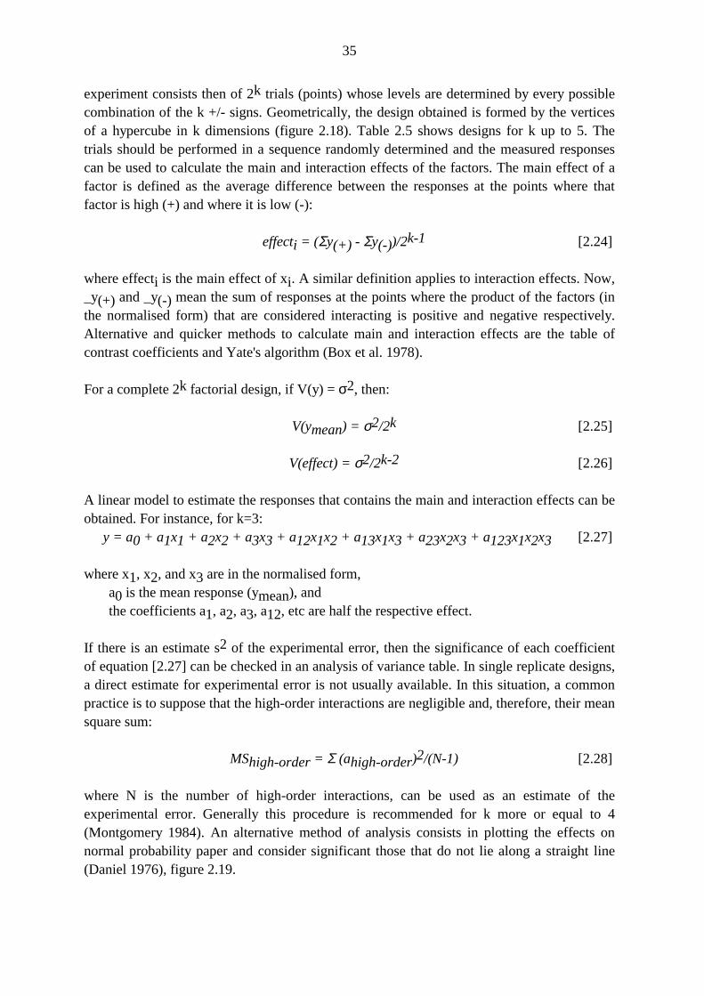
35
experiment consists then of 2k trials (points) whose levels are determined by every possiblecombination of the k +/- signs. Geometrically, the design obtained is formed by the verticesof a hypercube in k dimensions (figure 2.18). Table 2.5 shows designs for k up to 5. Thetrials should be performed in a sequence randomly determined and the measured responsescan be used to calculate the main and interaction effects of the factors. The main effect of afactor is defined as the average difference between the responses at the points where thatfactor is high (+) and where it is low (-):
effecti = (Σy(+) - Σy(-))/2k-1 [2.24]
where effecti is the main effect of xi. A similar definition applies to interaction effects. Now,_y(+) and _y(-) mean the sum of responses at the points where the product of the factors (inthe normalised form) that are considered interacting is positive and negative respectively.Alternative and quicker methods to calculate main and interaction effects are the table ofcontrast coefficients and Yate's algorithm (Box et al. 1978).
For a complete 2k factorial design, if V(y) = σ2, then:
V(ymean) = σ2/2k [2.25]
V(effect) = σ2/2k-2 [2.26]
A linear model to estimate the responses that contains the main and interaction effects can beobtained. For instance, for k=3:
y = a0 + a1x1 + a2x2 + a3x3 + a12x1x2 + a13x1x3 + a23x2x3 + a123x1x2x3 [2.27]
where x1, x2, and x3 are in the normalised form, a0 is the mean response (ymean), and the coefficients a1, a2, a3, a12, etc are half the respective effect.
If there is an estimate s2 of the experimental error, then the significance of each coefficientof equation [2.27] can be checked in an analysis of variance table. In single replicate designs,a direct estimate for experimental error is not usually available. In this situation, a commonpractice is to suppose that the high-order interactions are negligible and, therefore, their meansquare sum:
MShigh-order = Σ (ahigh-order)2/(N-1) [2.28]
where N is the number of high-order interactions, can be used as an estimate of theexperimental error. Generally this procedure is recommended for k more or equal to 4(Montgomery 1984). An alternative method of analysis consists in plotting the effects onnormal probability paper and consider significant those that do not lie along a straight line(Daniel 1976), figure 2.19.

36
There are many circumstances in which it is impossible to perform a complete 2k factorialdesign in one block, where a block may be a plate of steel, a laboratory or welding machine,etc. If the effect of the blocks can be assumed to be additive, it can be confounded with high-order interactions without affecting low-order interactions and main effects by using atechnique called confounding.The same approach can be used to obtain fractional factorial designs. These designs allow theexperimenter to study main effects and low-order interactions in fewer runs than required ina complete factorial design by sacrificing the high-order interactions. Fractional factorials areimportant when the number of factors is high and the high-order interactions are negligiblebecause they can offer a great economy of time and resources. Confounding and fractionatingof factorial experiments are thoroughly discussed in the literature (for instance, Box et al.1978, Montgomery 1984, and Box and Draper 1987).
2.4.3.3.Regression analysis
Linear regression analysis is a statistical technique for investigating and modelling therelationship between variables. Gauss, in about 1809, is usually considered to havedeveloped the method which changed very little until late 1950's, probably because of thelack of high-speed computing (Hocking 1983). Since then, the situation has dramaticallychanged and, nowadays, regression analysis is widely employed in almost every field and isone of the most commonly used statistical techniques. Regression models are used forseveral purposes, including (Montgomery and Peck 1982):
. data description,
. parameter estimation,
. prediction and estimation, and
. control.
The literature on regression analysis is enormous, including many textbooks (Draper andSmith 1981, Montgomery and Peck 1982, Weisberg 1985 and Rawlings 1988, for instance).The subject is also part of almost any textbook on applied statistics. The developments ofregression analysis were recently discussed by Hocking (1983). The present review will onlyintroduce the basic concepts and techniques associated with the method.
Regression analysis starts by postulating that a certain response y is adequately described bythe linear model with k input variables or predictors (xi):
∑=
+=k
iii xy
1εβ [2.29]
where ßi are unknown parameters and _ is the experimental error. For simplicity, the presentdiscussion considers that the response and predictors are centred, i. e., they were transformedby subtracting the mean from each variable. Consequently, y and xi (i= 1..k) have means
37
equal to zero and a b0 term (a constant) is not included in [2.29]. In order to examine thismodel a random sample of size n of predictors and response has to be obtained. The data andthe model are summarized in matrix notation as:
y = Xββββ + εεεε [2.30]
where y is a (nx1) vector of responses (see [2.22]), X is a (nxk) matrix of predictors (see [2.22]), ββββ is a (kx1) vector of unknown parameters, and εεεε is a (nx1) vector of errors.
It is assumed that the experimental error is independent and has constant variance, i. e.:
E(εεεε) = 0 and V(εεεε) = Iσσσσ2 [2.31a]
so:
E(y) = Xββββ [2.31b]
Accepting that the model adequately represents the data, estimates for the parameters in ββββhave to be obtained. In linear regression, the criterion used for parameter estimation is thatthe sum of the squared differences between the observed responses and the model predictionsshould be minimized. It can be shown that, if X'X is not singular, the linear regressionestimates are given by:
b = (X'X)-1X'Y [2.32]
and the fitted model and the residuals are respectively:
y) = Xb [2.33]
e = y - y) [2.34]
The linear regression vector of estimates (b) has the following properties (Draper and Smith1981):
. it is an estimate of ββββ that minimizes _'_ irrespective of any distribution propertiesof the errors,
. the elements of b provide unbiased estimates of the elements of ββββ which haveminimum variances irrespective of distribution properties of the errors, and
. if the errors follow a normal distribution, b is also the maximum likelihoodestimate of ββββ.
38
If it can be further assumed that the errors follow a normal distribution, the regression modelcan be tested by an analysis of variance table to check if the coefficients b can be consideredequal to a certain vector b0. If b0 is the null vector, the test is called a test for significance ofregression. This test determines if it is reasonable to assume a linear relationship between theresponse and any regressor (table 2.6). If replicated runs are available, the model can also betested for lack of fit (table 2.7).
The coefficient of multiple determination R2 is frequently used as a measure of the fractionof variation of y that is explained by the regressor variables. However R2 will alwaysapproach one when a predictor is added to the model. So, model with large number ofpredictors will tend to have high values of R2 without any guarantee of performing well inprediction.
Analysis of the residuals plays an important role in judging model adequacy. It is basically agraphical method with several types of plot being used:
. histogram of residuals,
. normal probability plot,
. time sequence plot,
. residuals versus fitted values ( y) i),
. residuals versus each regressor, and
. residuals versus regressors not included in the model.
Plotting residuals can help to detect outliers and violations of the assumptions about theerrors. Several numerical tests also exist for regression diagnostics (see, for instance,Weisberg 1985, chapter 5).Transformations of the response or predictors can be used for reducing either nonconstantvariance or nonlinearity (lack of fit). Also, errors in the transformed regression may be morenormally distributed than the errors in the untransformed case. A transformation may alsoallow the use of a simpler model to describe the data. Transformations can be selected eitherempirically or theoretically (Box and Draper 1987). A power transformation is commonlyused for the response:
ytrans = yt [2.35]
A best value for t can be interactively determined by maximizing the likelihood function(Box and Cox 1964):
L(t) = -(n/2)ln(SSet) + n(t - 1)ln(ygm) [2.36]
or minimizing the mean square error for regression models using the transformation below:
(yt – 1) / (t ygmt-1) t ≠ 0
zt = [2.37] ygm ln(y) t = 0

39
where L(t) is the log-likelihood function, n is the number of data points, SSet is the residual sum of squares, and ygm is the geometric mean of the y's.
The method discussed above should be used cautiously because it can be highly inefficient ifthe distribution of errors has heavier tails than the normal distribution and it is very sensitiveto outliers (Carrol and Ruppert 1985).
An approximate 100(1 - α) percent confidence interval on t can be calculated by(Montgomery and Peck 1982):
SS* = SSet.[1 + (t / 2,v2)/v] [2.38]
Where v = n - k - 1 is the number of residual degrees of freedom, and t_/2,v is the upper α/2 percentage point of the t distribution with v degrees offreedom. The confidence interval is then obtained by finding the points where the horizontalline SS* intercepts the curve of SSet against t.
Predictor variables can be transformed to describe maxima and minima in the response (forinstance, by including powers of predictors to model the response) or to accommodatenonlinearity.
In many applications, there are a number of candidate variables that may or may not beimportant for the model. The problem of finding an appropriate subset of regressors is called"variable selection" or "selection of the best regression equation". Two important aspects ofvariable selection are generating candidate models and selecting which candidate is betterthan others. Some possible criteria for model selection are:
. Coefficient of multiple determination.
. Adjusted R2.
. Residual mean square (MSr).
. Mallows' Cp statistic.
. Partial F ratio
The main computational techniques for variable selection can be grouped as (Montgomeryand Peck 1981, and Nie et al. 1975):
. All possible regressions: All possible combinations containing the predictors arefitted and the best model is selected by some statistical criteria.
. Forward inclusion: The procedure begins with the assumption that there are nopredictors in the model. Variables are, then, entered in the model only if they
40
meet certain criteria. The order of inclusion is determined by the respectivecontribution of each variable to improve the model.
. Backward elimination: The procedure starts with a model including all possiblepredictors. Those predictors that do not meet some criteria are eliminated one byone from the model.
. Stepwise selection: This process is a modification of forward elimination inwhich at each step all predictors already in the model are checked by their partialF ratio. A regressor is dropped from the model if their partial F ratio is less than acritical value (FOUT). The process finishes when no variable can be either addedor dropped from the model.
The primary limitations of variable selection techniques are that (a) the procedure implies anorder of importance to the variables, an order that may be misleading or confusing, (b) incase of early termination or the presence of collinearity, the procedure may fail to detectimportant variables, and (c) different selection techniques and criteria can result in different"best" models for the same set of data (Hocking 1983).
When all the predictors variables are orthogonal or independent, i. e., any two columns Xiand Xj (i # j) of the data matrix X has inner product nought (Xi.Xj = 0), the use andinterpretation of linear regression is relatively easy. In many cases the regressors are notorthogonal. When there is a nearly perfect linear relation among the predictor variables, theproblem called "collinearity" exists. The consequences of collinearity are: (a) coefficientestimates tend to inflate and may have incorrect sign, (b) predicted values may beunreasonable, and (c) the stepwise, backward and forward variable selection methods can failto detect important combinations of variables. Some techniques to deal with collinearity are(Montgomery and Peck 1984, Hocking 1983):
. Collection of additional data,
. model respecification,
. elimination of some variables when the collinearity is inherent to the system, and
. use some alternative estimation technique, such as Ridge regression, capable ofprovide some alternative estimator that is biased but could have a lower variancethan the linear regression estimator.
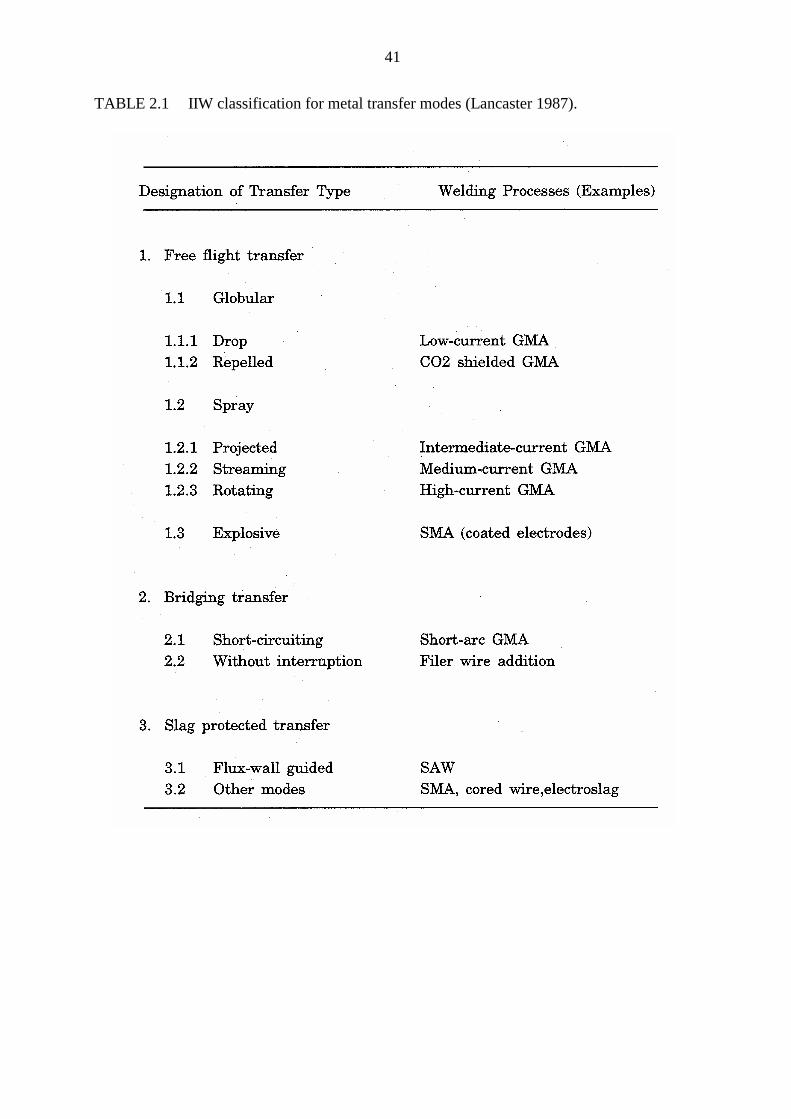
41
TABLE 2.1 IIW classification for metal transfer modes (Lancaster 1987).
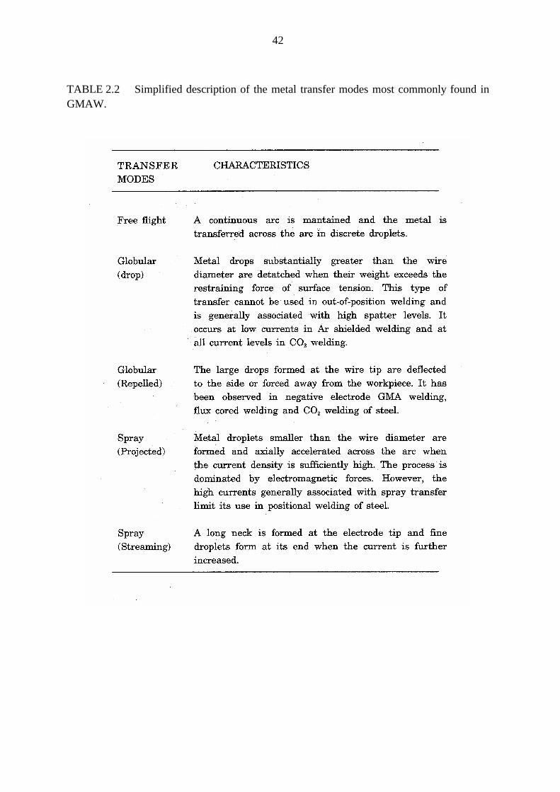
42
TABLE 2.2 Simplified description of the metal transfer modes most commonly found inGMAW.

43
TABLE 2.2(con) Simplified description of the metal transfer modes mostcommonly found in GMAW.
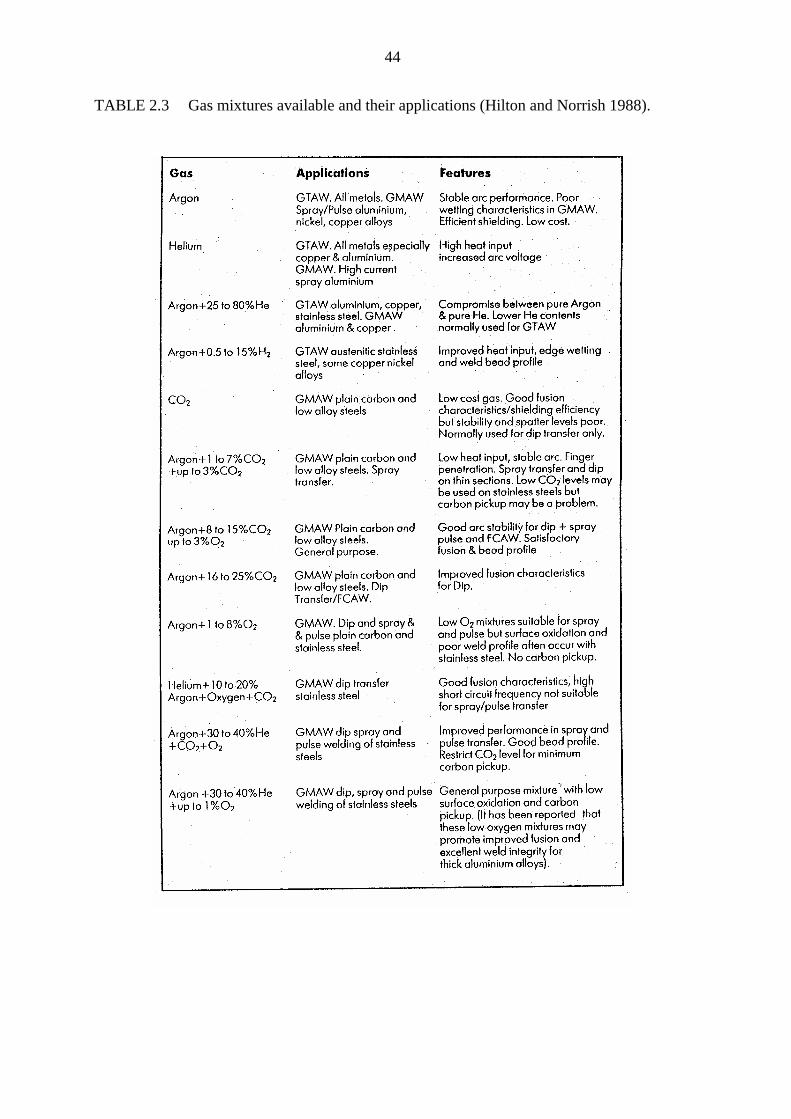
44
TABLE 2.3 Gas mixtures available and their applications (Hilton and Norrish 1988).
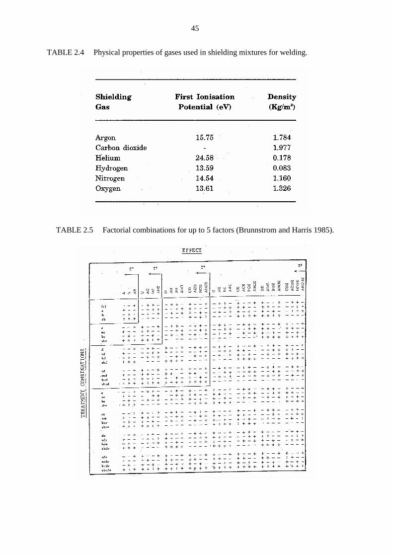
45
TABLE 2.4 Physical properties of gases used in shielding mixtures for welding.
TABLE 2.5 Factorial combinations for up to 5 factors (Brunnstrom and Harris 1985).
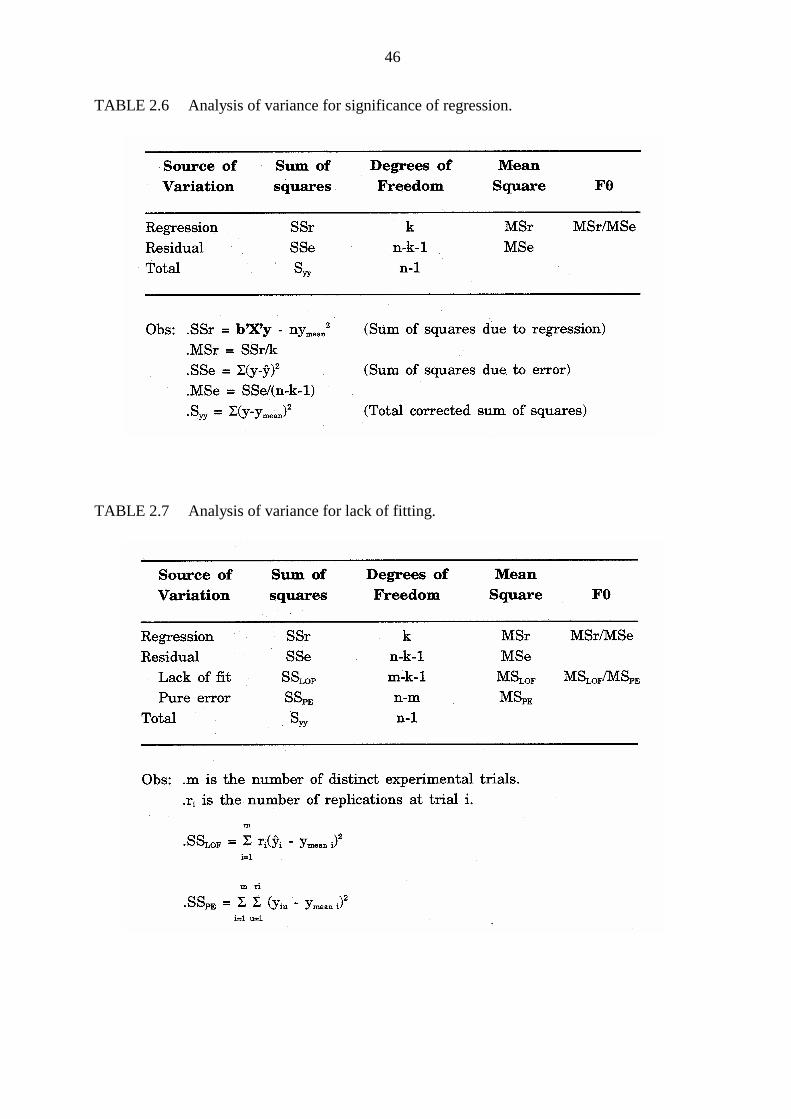
46
TABLE 2.6 Analysis of variance for significance of regression.
TABLE 2.7 Analysis of variance for lack of fitting.
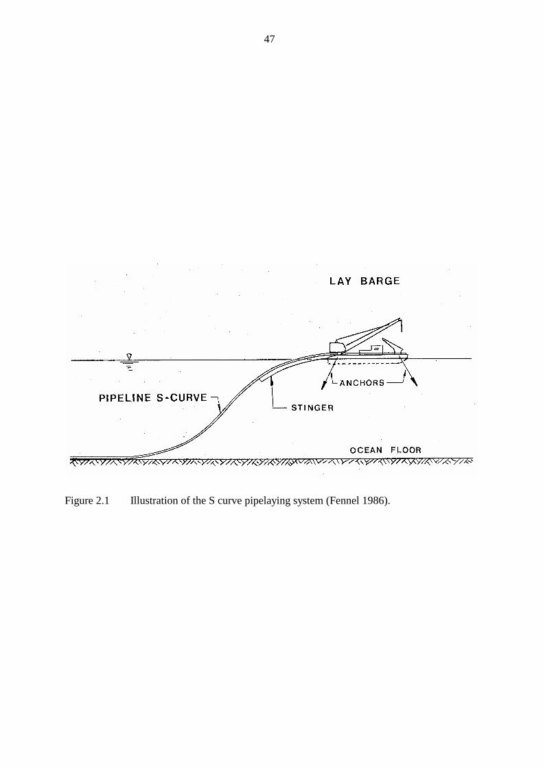
47
Figure 2.1 Illustration of the S curve pipelaying system (Fennel 1986).
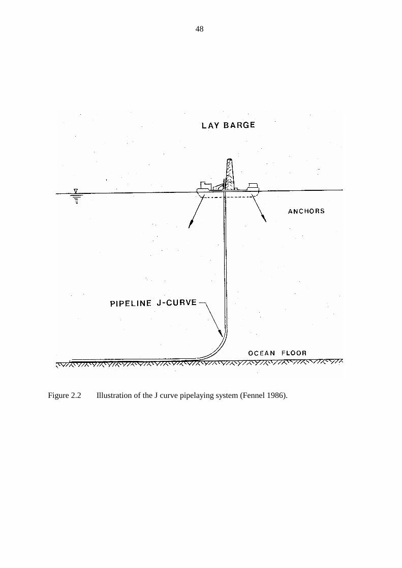
48
Figure 2.2 Illustration of the J curve pipelaying system (Fennel 1986).
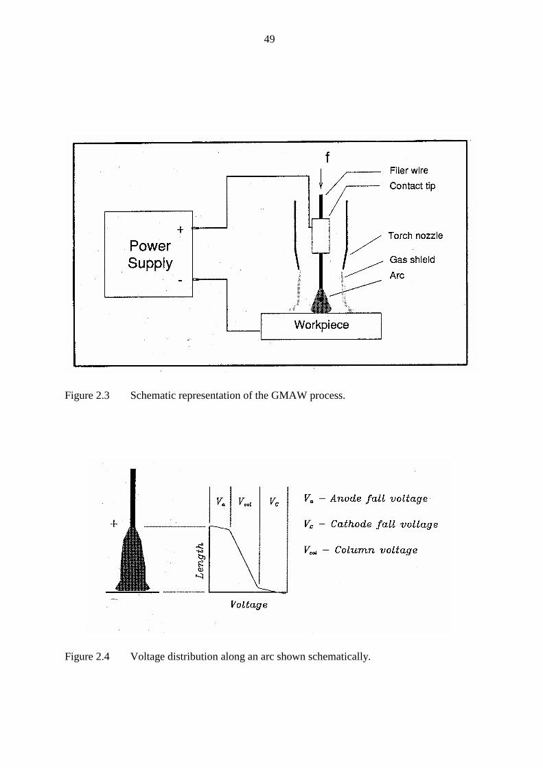
49
Figure 2.3 Schematic representation of the GMAW process.
Figure 2.4 Voltage distribution along an arc shown schematically.
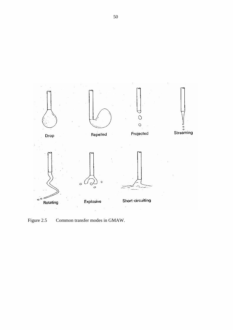
50
Figure 2.5 Common transfer modes in GMAW.
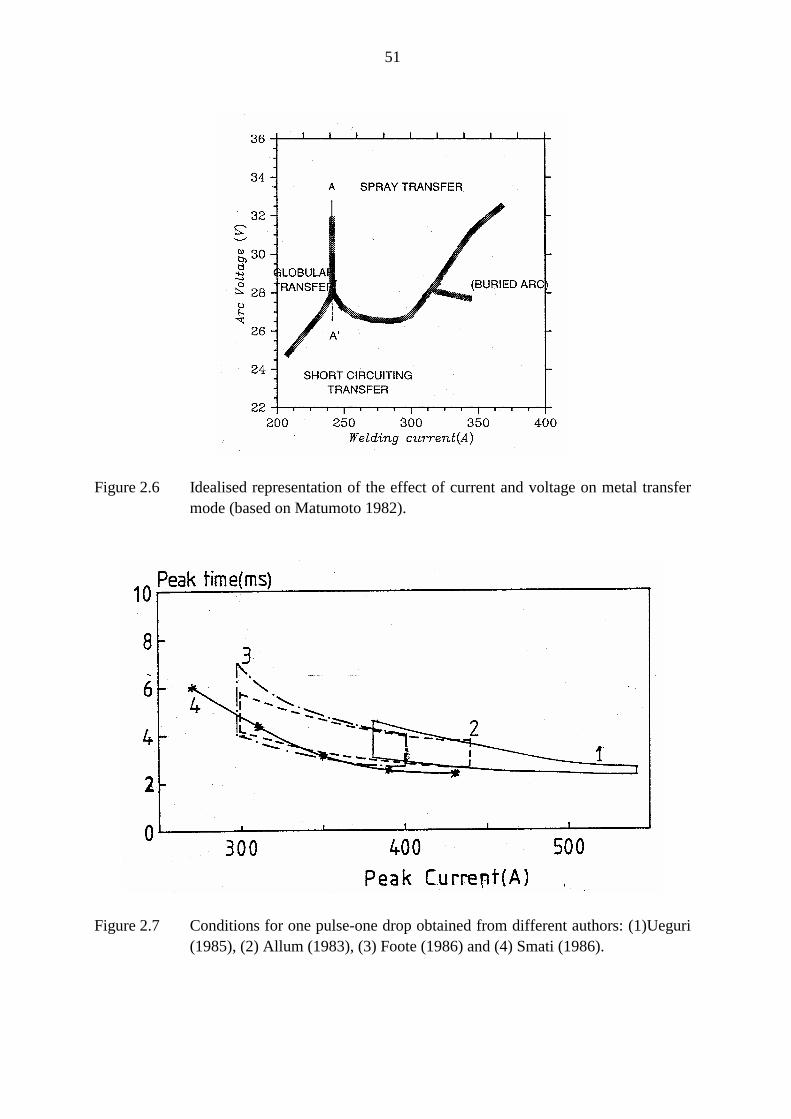
51
Figure 2.6 Idealised representation of the effect of current and voltage on metal transfermode (based on Matumoto 1982).
Figure 2.7 Conditions for one pulse-one drop obtained from different authors: (1)Ueguri(1985), (2) Allum (1983), (3) Foote (1986) and (4) Smati (1986).
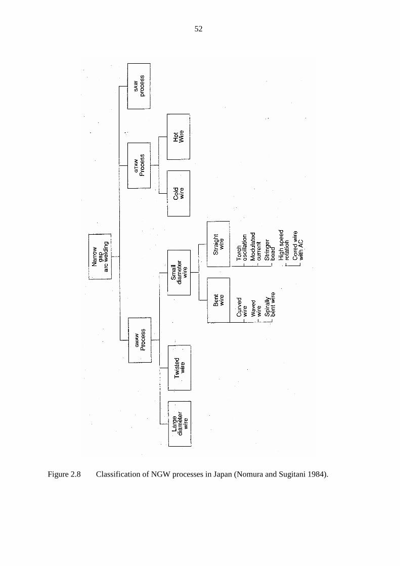
52
Figure 2.8 Classification of NGW processes in Japan (Nomura and Sugitani 1984).
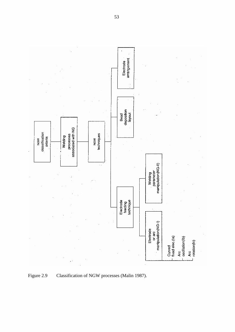
53
Figure 2.9 Classification of NGW processes (Malin 1987).
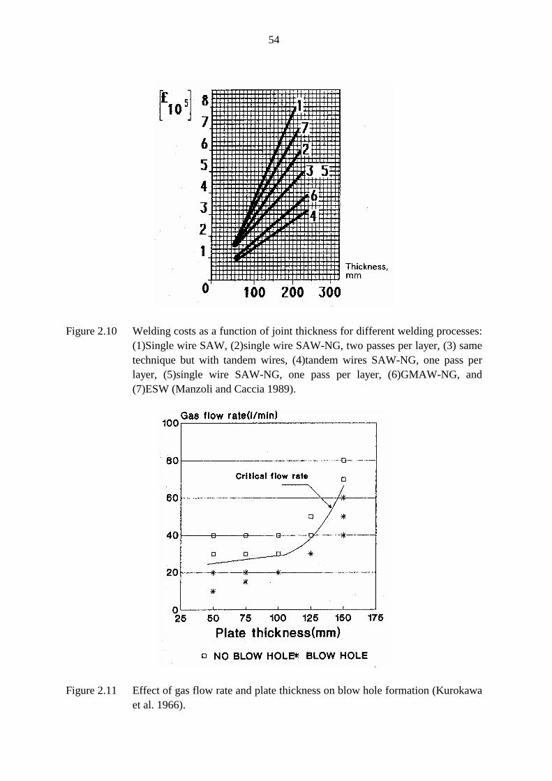
54
Figure 2.10 Welding costs as a function of joint thickness for different welding processes:(1)Single wire SAW, (2)single wire SAW-NG, two passes per layer, (3) sametechnique but with tandem wires, (4)tandem wires SAW-NG, one pass perlayer, (5)single wire SAW-NG, one pass per layer, (6)GMAW-NG, and(7)ESW (Manzoli and Caccia 1989).
Figure 2.11 Effect of gas flow rate and plate thickness on blow hole formation (Kurokawaet al. 1966).
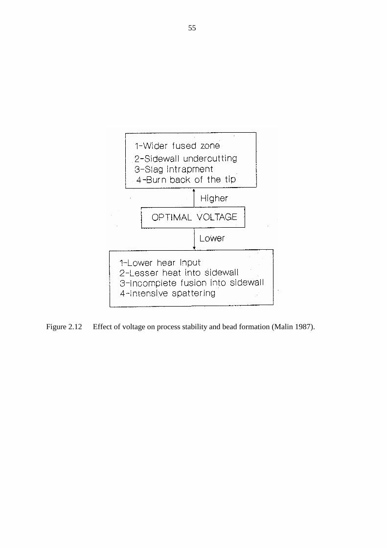
55
Figure 2.12 Effect of voltage on process stability and bead formation (Malin 1987).
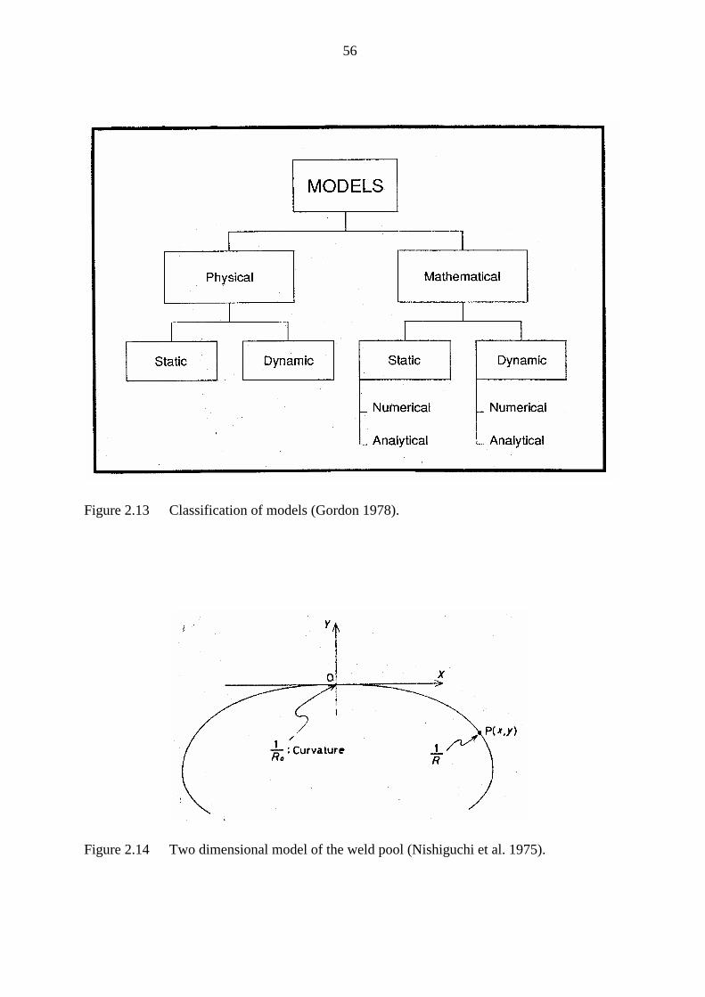
56
Figure 2.13 Classification of models (Gordon 1978).
Figure 2.14 Two dimensional model of the weld pool (Nishiguchi et al. 1975).
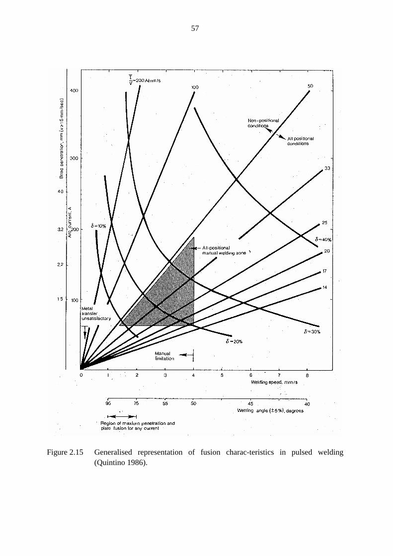
57
Figure 2.15 Generalised representation of fusion charac-teristics in pulsed welding(Quintino 1986).
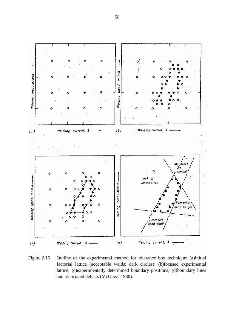
58
Figure 2.16 Outline of the experimental method for tolerance box technique: (a)Initialfactorial lattice (acceptable welds: dark circles); (b)focused experimentallattice; (c)experimentally determined boundary positions; (d)boundary linesand associated defects (McGlove 1980).
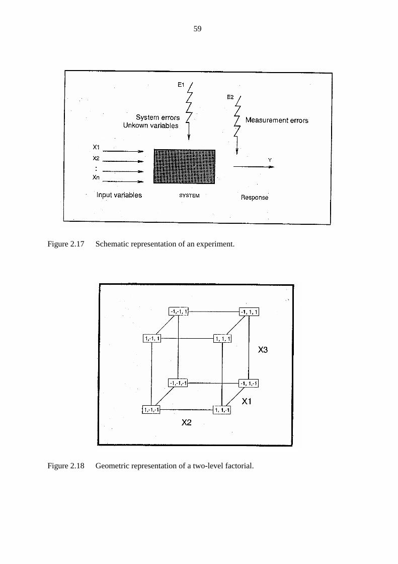
59
Figure 2.17 Schematic representation of an experiment.
Figure 2.18 Geometric representation of a two-level factorial.
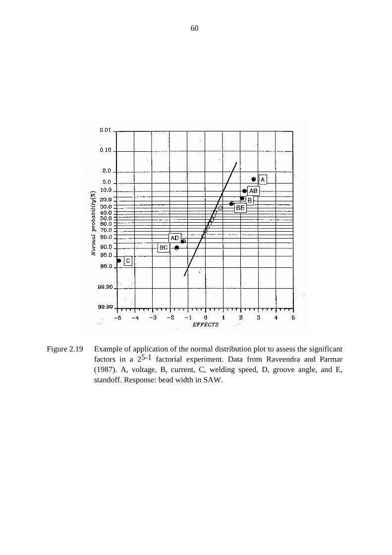
60
Figure 2.19 Example of application of the normal distribution plot to assess the significantfactors in a 25-1 factorial experiment. Data from Raveendra and Parmar(1987). A, voltage, B, current, C, welding speed, D, groove angle, and E,standoff. Response: bead width in SAW.

CHAPTER 3

62
3. EQUIPMENT AND MATERIALS
3.1.Power supplies
Two electronic power supplies were used during most of the experimental work: a TPSFronius 500 and a GEC (AWP) M500. A special GEC series regulator power supplycommissioned by the Cranfield Institute of Technology was used for a few trials in thehyperbaric chamber.
3.1.1.TPS Fronius 500
The TPS Fronius 500 is a high frequency (25 KHz) primary inverter power supply. It is ahighly flexible machine that uses microprocessor control and is based on a modular systemstructure. Different control boxes provide different operation modes including severalsynergic GMAW programmes and CVCC operation. In the present work, the Tr-17 controlbox which allows independent control of all pulse parameters was used. This power supplywas used for pulsed current welding.
3.1.2.GEC (AWP) M500
This is a series regulator type power supply. Its main technical characteristics are listed intable 3.1. This power supply was used for constant current (non-pulsing) welding.
3.2.Wire feed unit
A Fronius Vr 130 wire feeder was used in conjunction with the TPS Fronius 500 powersupply. It provides a wire feed speed continuously adjustable between 0-18 m/min. A digitaldisplay with a resolution of 0.1 m/min indicates the selected wire feed speed.
An ESAB A10-MEC44 feeder was used in conjunction with the GEC (AMP) M500 powersupply. Originally, the wire speed was selected and indicated by a low resolution andunreliable marked dial. This was improved by using the voltage signal from the speed controlpotentiometer of the wire feeder to indicate the wire speed. For both wire feeders, the actualwire speeds were calibrated against the selected values (figure 3.1).
3.3.Welding torch
An AW 500 torch was used with the Fronius power supply. Approximately 3 mm wasmachined from the gas shroud to expose the contact tip for narrow gap welding. A UnionCarbide ST12 water cooled torch was used with the GEC (AWP) M500 power supply.
63
3.4.Test rig
The welding rig consisted of a table that could be moved in the horizontal direction while thetorch was kept fixed. A simple support was built and attached to the table for positionalwelding (figure 3.2). The horizontal position and height of the torch were controlled bymeans of manually adjustable lead screws. The welding position was changed by rotating thetorch along an axis parallel to the welding direction. The travel speed of the welding tablewas calibrated before its use (figure 3.3). A schematic diagram of the welding rig andmeasuring equipment is shown in figure 3.4. The video equipment shown in this figure wasused for measuring the arc length in some welding trials.
3.5.Gas mixer and analyser
Two gas mixing devices were used throughout the project to add different proportions ofoxygen to commercial shielding gases: a Witt gas mixer was used in the initial stages of theproject (shielding gas optimization) and a Cranfield built mixer (figure 3.5) was employed inthe modelling of narrow gap welding with the optimized mixture. Both mixers operatedusing similar principles, i. e., the gases are supplied from high pressure cylinders with acontrolled flow and mixed in a chamber before being fed into the welding torch. Thecomposition of the output mixture was defined by the composition and relative flow of the ninput gases:
∑∑==
=n
jj
n
jijji fcfc
11
/)( [3.1]
where ci is the content of component i in the output mixture, fj is the flow of the input mixture j, and cij is the content of i in the input mixture j.
The flow of the input gases was monitored and controlled by tapered tube and float devicesplaced at the entrances of the mixing chamber. As different commercial gas mixtures wereused with flowmeters calibrated for either argon or helium, the actual gas flow (fact) wascalculated from the measured flow (fmeas) by:
fact = fmeas.(σref / σact)0.5 [3.2]
where σref and σact are the densities of the reference and actual gases respectively. Thedensities of gases relevant to the present work are shown in table 2.4.
A Servomex 1420 oxygen analyser (Servomex 1987) was used with the Witt mixer to checkthe oxygen concentration in the output gas mixture. The same analyser was utilized tocalibrate the Cranfield built mixer.

64
3.6.Photography
The equipment and some weld beads were photographed with ordinary 35 mm black andwhite film. Weld bead macro-photographs were taken using a Vickers microscope using100x120 mm negatives. Metal transfer and arc shape were photographed using both an"Imacon" image converter camera (time between exposures of 0.100 msec) with back flashillumination and Polaroid film, and an ordinary reflex 35 mm camera with 1/2000 shutterspeed, 210 mm lens and extension tube. Neutral density filters were used to reduce the arcglare.
3.7.Current and voltage measurement
Mean current and voltage were measured using the built-in digital meters in the powersupplies. These meters presented a resolution of 1A and 0.1 V in both power supplies andtheir calibration was checked against other meters previously calibrated with a precisionpower supply.
For the analysis of the pulse structure in pulsed current welding and the study of weldingcurrent and voltage transient phenomena, a digital data logger (VELA) was used to registersignals from these parameters. The VELA is a simple to operate and flexible 8-bit datalogger with 4k of RAM memory and 1 or 4 channels manufactured by Data Harvest. The datastored in the VELA can be transferred to a BBC microcomputer by a programme supplied byData Harvest and called Vela Analysis which can also plot graphs, measure instantaneousvalues and store the data on disk for further analysis.
3.8.Metallographic equipment
Macrographic specimens were sectioned on a band saw and prepared using rotating siliconcarbide papers up to 1200 mesh. Nital 10% (nitric acid in alcohol) was used as etchant. AVickers projection microscope was used to produce magnified tracings (4-7X) of thespecimens.
3.9.Weld bead measurement
Two methods were used to determine the weld bead dimensions:
- A planimeter and a ruler were used to measure areas and linear dimensionsrespectively in magnified tracings of the weld bead.
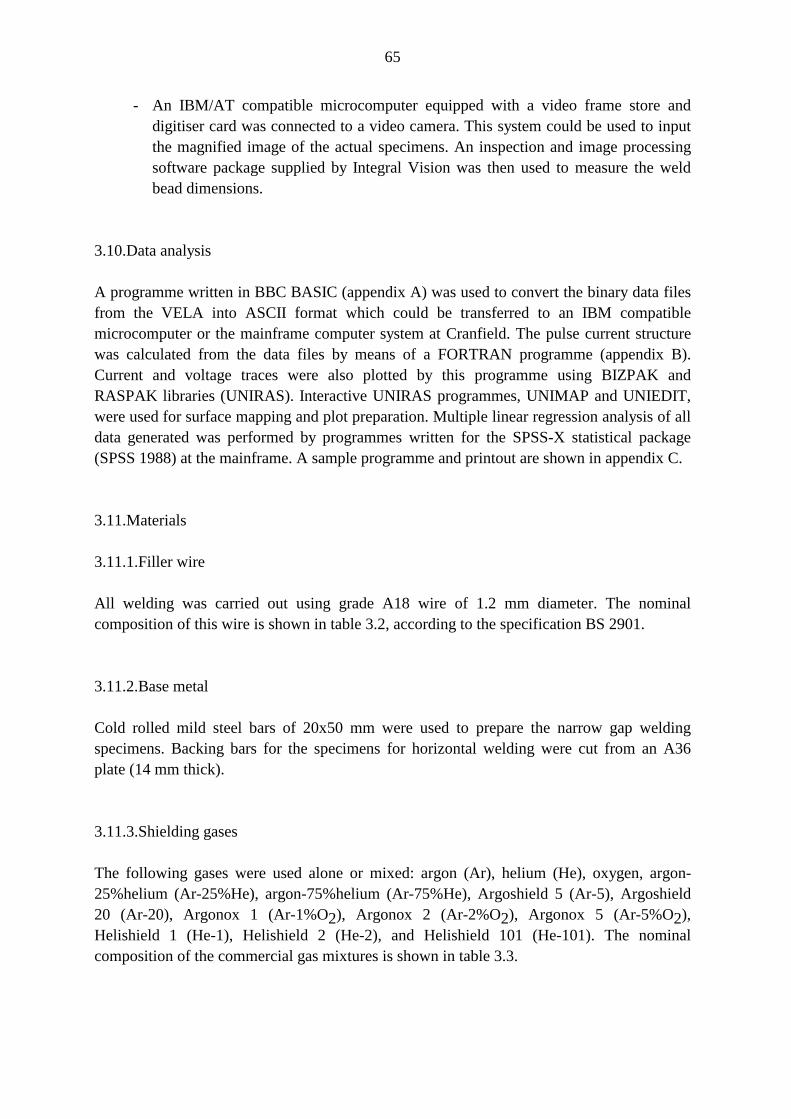
65
- An IBM/AT compatible microcomputer equipped with a video frame store anddigitiser card was connected to a video camera. This system could be used to inputthe magnified image of the actual specimens. An inspection and image processingsoftware package supplied by Integral Vision was then used to measure the weldbead dimensions.
3.10.Data analysis
A programme written in BBC BASIC (appendix A) was used to convert the binary data filesfrom the VELA into ASCII format which could be transferred to an IBM compatiblemicrocomputer or the mainframe computer system at Cranfield. The pulse current structurewas calculated from the data files by means of a FORTRAN programme (appendix B).Current and voltage traces were also plotted by this programme using BIZPAK andRASPAK libraries (UNIRAS). Interactive UNIRAS programmes, UNIMAP and UNIEDIT,were used for surface mapping and plot preparation. Multiple linear regression analysis of alldata generated was performed by programmes written for the SPSS-X statistical package(SPSS 1988) at the mainframe. A sample programme and printout are shown in appendix C.
3.11.Materials
3.11.1.Filler wire
All welding was carried out using grade A18 wire of 1.2 mm diameter. The nominalcomposition of this wire is shown in table 3.2, according to the specification BS 2901.
3.11.2.Base metal
Cold rolled mild steel bars of 20x50 mm were used to prepare the narrow gap weldingspecimens. Backing bars for the specimens for horizontal welding were cut from an A36plate (14 mm thick).
3.11.3.Shielding gases
The following gases were used alone or mixed: argon (Ar), helium (He), oxygen, argon-25%helium (Ar-25%He), argon-75%helium (Ar-75%He), Argoshield 5 (Ar-5), Argoshield20 (Ar-20), Argonox 1 (Ar-1%O2), Argonox 2 (Ar-2%O2), Argonox 5 (Ar-5%O2),Helishield 1 (He-1), Helishield 2 (He-2), and Helishield 101 (He-101). The nominalcomposition of the commercial gas mixtures is shown in table 3.3.

66
3.12.Narrow gap welding specimen preparation
Linear specimens were used throughout the experimental programme since they are cheaperand easier to prepare, and simulate closely a short length of a tubular joint. Additionally,positioning of the welding torch in the joint and controlling its position during welding aresimpler when using a linear specimen.
The mild steel bars were degreased, cut into pieces approximately 250 mm and 280 mm long(for the specimen's sides and backing bar respectively), and bright ground. A diagram of thespecimen is presented in figure 3.6. Machined spacers were placed into the groove duringspecimen assembly in order to ensure the correct gap width required for each specimen.Thinner backing bars (15 mm) with holes drilled at its extremities were used in specimensfor the horizontal-vertical welding trials.

67
Table 3.1 Technical specifications of the M500 power supply (Foote 1986).
__________________________________________________________________________
Input:Voltage: 380/400 V - 3 phaseFrequency: 50 Hz
Output:Open circuit voltage: 55 V
Characteristics:
- Output current/voltage relationship infinitely variable between constant current andconstant voltage.
- Current level variable between 0 - 500 A in 1A steps.
- Current rise time variable between 0.1 - 10 ms in 0.1 ms steps.
- Short circuit current variable between 0 - 499 A with variable short circuit detectvoltage.
- Peak and background levels between 0 - 500 A in 1 A steps.
- Accuracy ±0.5%.
- Peak and background duration between 0 - 999.9 ms in 0.1 ms steps.
- Reproducibility and accuracy:current: ±1% at full scale setting,timing: ±0.5% for each control.
__________________________________________________________________________

68
Table 3.2 Chemical composition of the filler wire (nominal).
C Mn Si S P
0.12 max 0.60-0.90 0.70-1.20 0.04max 0.040max
Table 3.3 Composition of commercial gas mixtures.
Mixture Nominal composition
Argoshield 5Argoshield 20Argonox 1Argonox 2Argonox 5Helishield 1Helishield 2Helishield 101
Ar-5% CO2-up to 2% O2Ar-20% CO2-up to 2% O2Ar-1% O2Ar-2% O2Ar-5% O2Ar-85% He-1.5% CO2-250Vpm O2Ar-75% HeAr-38% He-2% CO2
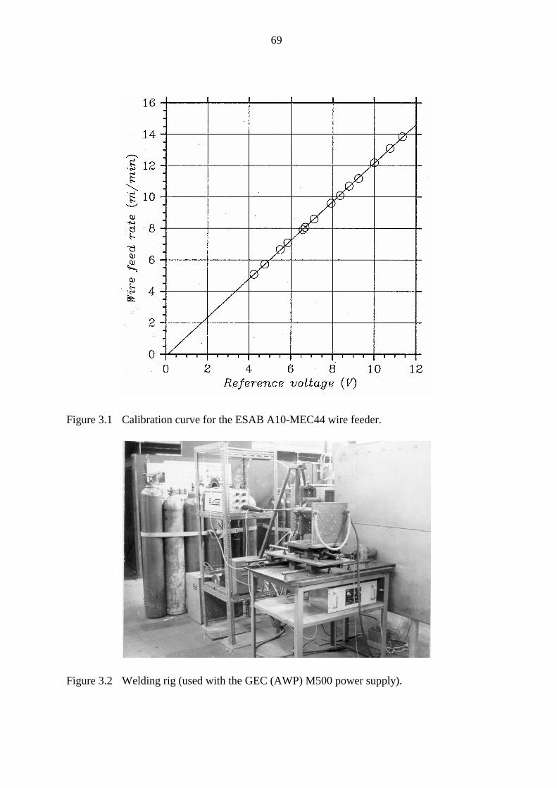
69
Figure 3.1 Calibration curve for the ESAB A10-MEC44 wire feeder.
Figure 3.2 Welding rig (used with the GEC (AWP) M500 power supply).
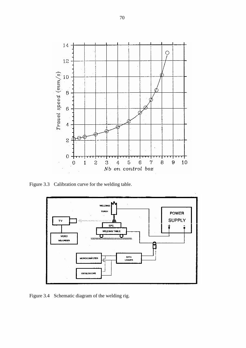
70
Figure 3.3 Calibration curve for the welding table.
Figure 3.4 Schematic diagram of the welding rig.
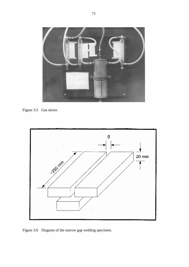
71
Figure 3.5 Gas mixer.
Figure 3.6 Diagram of the narrow gap welding specimen.

CHAPTER 4

73
4. RESEARCH PROGRAMME
The J-laying technique for the construction of offshore pipelines requires a fast weldingprocess that can produce sound welds in the horizontal-vertical position. A previous projectat the Cranfield Institute of Technology (Fennel 1986) demonstrated for that application thesuitability of a NG-GMAW process with the following characteristics:
- NGW II technique (§2.31),- reduced gap width (under 9mm),- thin wire diameter,- DC+ pulsed current operation, and- high welding speed.
However, an extensive study which could provide a better understanding of the relationshipbetween process variables and the physical processes involved in the formation of the weldbead in this process had not been carried out. Previous work in narrow gap welding isgenerally associated with the NGW I technique or with wire diameters and current levelsmuch higher than those which can be used in the horizontal-vertical position. This studyshould provide valuable information to help establishing improved welding conditions forthe process in terms of minimizing the likelihood of defect formation and optimizing thewelding time.
As a result, the basic aims of the experimental programme were as:
- to investigate the influence of welding parameters on bead characteristics in anarrow gap GMAW process to be applied to the welding of pipelines in the J-curvepipelaying technique,
- to establish a set of optimal welding conditions for this process based on somecriteria and to determine the sensitivity of these conditions to small variations inprocess parameters, and
- to determine the most significant parameters that control bead shape in a narrow gapprocess.
Statistical modelling of the welding process was used throughout the programme in order toaccomplish these aims. Statistical principles were used for both design of the experimentalwork, data analysis and modelling. This approach was considered more efficient than eitherthe classical "one-variable-at-a-time" experimental approach or purely theoretical modellingto cope with the complexity and large number of variables of the process.
Results from initial experimental work indicated arc instability problems associated with thecommercial helium based shielding mixture. These problems tended to occur only for the
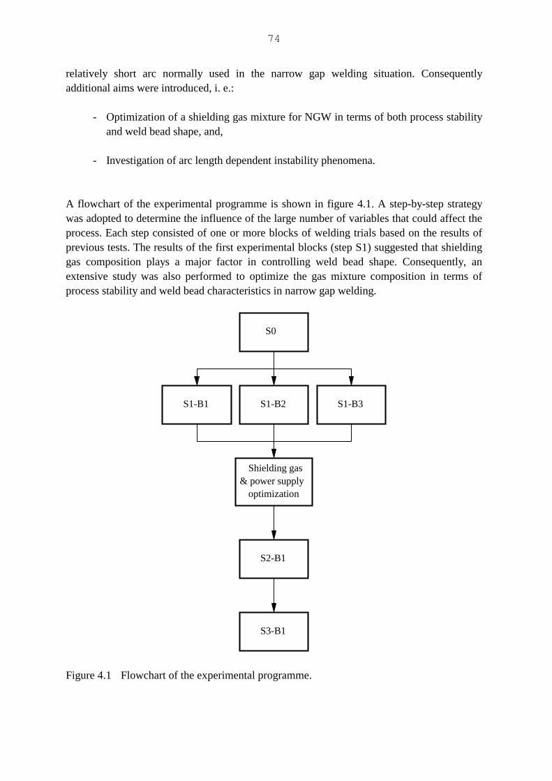
74
relatively short arc normally used in the narrow gap welding situation. Consequentlyadditional aims were introduced, i. e.:
- Optimization of a shielding gas mixture for NGW in terms of both process stabilityand weld bead shape, and,
- Investigation of arc length dependent instability phenomena.
A flowchart of the experimental programme is shown in figure 4.1. A step-by-step strategywas adopted to determine the influence of the large number of variables that could affect theprocess. Each step consisted of one or more blocks of welding trials based on the results ofprevious tests. The results of the first experimental blocks (step S1) suggested that shieldinggas composition plays a major factor in controlling weld bead shape. Consequently, anextensive study was also performed to optimize the gas mixture composition in terms ofprocess stability and weld bead characteristics in narrow gap welding.
Shielding gas& power supply
optimization
S0
S1-B1 S1-B2 S1-B3
S2-B1
S3-B1
Figure 4.1 Flowchart of the experimental programme.

CHAPTER 5
76
5. PROCESS MODELLING
5.1.Experimental procedure
5.1.1.Design of the experiments
The experimental programme was intended to produce data for statistical modelling of thenarrow gap GMAW process. Whereas theoretical model building is based mainly onconsiderations about basic physical or chemical principles, statistical modelling dependssolely on information contained in the experimental data it is being applied to. Therefore aproperly designed and conducted experiment is crucial for the modelling exercise to succeed.Definition and statement of the problem, gathering of expertise and the execution ofexploratory trials to define system behaviour are an essential initial stage.
The present programme was run as a set of experimental steps. Each step was formed by oneor more experimental blocks which, in turn, were constituted by a number of welding trials.A sequential approach was used so that the results from one step could influence the designof the following step. A certain bias between experimental steps can result from thisapproach, but it was considered the most flexible to cope with the large number of variablesinvolved in the study and with the exploratory nature of the optimization process.
An extensive list of factors that can have some influence on bead shape in a narrow gap IIprocess is shown in table 5.1. Not all of the factors listed there are independent of each otherand different relationships may exist between two or more of them. Some relationships arequite obvious, such as (table 5.1):
h = s + la [5.1]
or
Imean = (Iptp + Ibtb)/(tp + tb) [5.2]
Others, however, can be much less obvious and more difficult to detect. Several weldingparameters, such as wire feed rate, welding current, voltage and shielding gas composition,must be inter-related in order to guarantee an acceptably stable operation for the process.Such constraint restricts the combinations of independent variable levels that can be possiblyused for studying the process and tend to introduce a certain level of dependency amongstpredictors. The division of the modelling and optimization problem into smaller units (steps
77
and blocks), as adopted in the present work, can reduce the problem by allowing fewerparameters to be analysed in each step and, therefore, reducing the quantity of constraints onthe experiment.
It was initially intended to design the experimental blocks as 2k factorial experiments withcentral points. This design was selected because it provides an efficient way to investigatethe effects and interactions of many variables with a relatively small number of experimentaltrials. A limitation of 2k factorial design is that no second or higher order effect can beobtained from it. However, as the experimental blocks were performed on a small region ofthe predictors space (i. e., only relatively small changes in the predictor variables were usedin each experimental block), an approximately linear relationship between predictors andresponse may be expected. Furthermore, if, after processing the data, the necessity of a morecomplicated model becomes apparent, the factorial experiment can be easily augmented tomore sophisticated designs.
However, results from the first experimental blocks indicated that, due to the strong inter-relationship amongst process variables, stable welding conditions were difficult to achievefor all experimental points when a factorial approach was used. Therefore the experimentaldesign was modified and a certain dependency between some of the predictor variablesallowed in the last two experimental steps.
5.1.2.Initial welding trials
An initial experimental step (figure 4.1, step S0) was performed to study the consistency ofweld bead shape along the length of a pass and amongst welds executed under similarconditions. The welding parameters used in this step were based on results from a previouswork (Fennel 1986) and are shown in table 5.2. A two pass weld was deposited on eachspecimen: the root pass extended along the entire length of the joint whereas the second passwas restricted to the first half of the joint. The welded specimen was cut into severaltransverse slices which were prepared for macrographic examination and measurement ofweld bead characteristics. The thickness of each slice was measured so that its position alongthe joint could be calculated approximately.
5.1.3.Modelling steps
The main body of the experimental part of the modelling work comprised three experimentalsteps (S1, S2 and S3, figure 4.1). The primary goal of step S1 was to study the process
78
response to changes in welding conditions around the initial points used in step S0 for threecommercial shielding gas mixtures (Ar-5, He-1 and Ar-20). Consequently, threeexperimental blocks were designed as 2k factorial experiments with central points. Wire feedrate, welding speed, gap width and a pulse parameter (either pulse frequency or backgroundcurrent level) were used as input factors (tables 5.3, 5.4 and 5.5).
A "customised factorial" experiment was adopted in step S2 in order to allow somecorrelation between wire feed rate and welding current. Based on results of experimental stepS1 and the shielding gas/process optimization step (chapter 7), step S2 used an experimentalshielding mixture together with a constant current (DC+) power supply. The predictorvariables in this step were welding current, wire feed rate, welding speed and gap width(table 5.6). When unmodulated arc current was used in this experimental block, its value wasalways kept above the globular-spray transition (230-250A for a 1.2mm mild steel wire).
The same shielding mixture and power supply characteristic were employed in step S3 (table5.7) in which the effect of the force of gravity (horizontal-vertical welding) was considered.
5.1.4.Complementary trials
A number of trials were performed after completion of blocks S2-B1 and S3-B1 in order toeither study the effect of some variables not included in the blocks, or to obtain multipassspecimens (table 5.8).
5.2.Experimental results
Many different dependent variables were considered at some stage of this programme inorder to explore different characteristics of the welding process (table 5.9).
5.2.1.Pulsed current parameters
In experimental steps S0 and S1, the current structure was calculated from data files recordedby VELA (§3.7) using a specially designed FORTRAN programme (appendix b). In somecases the current trace could include a significantly high noise level due to the current controlmechanism of the power supply, and the data was filtered in the software before being used
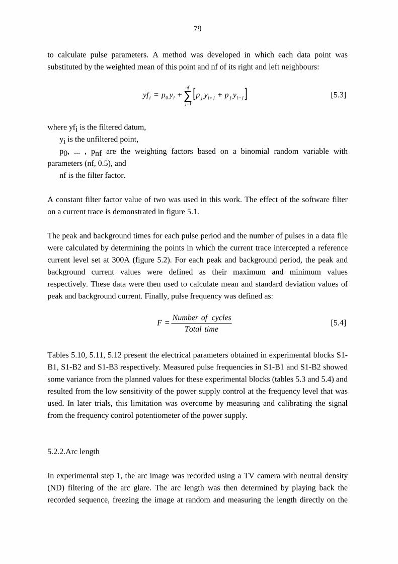
79
to calculate pulse parameters. A method was developed in which each data point wassubstituted by the weighted mean of this point and nf of its right and left neighbours:
[ ]∑=
−+ ++=nf
jjijjijii ypypypyf
10 [5.3]
where yfi is the filtered datum, yi is the unfiltered point, p0, ... , pnf are the weighting factors based on a binomial random variable withparameters (nf, 0.5), and nf is the filter factor.
A constant filter factor value of two was used in this work. The effect of the software filteron a current trace is demonstrated in figure 5.1.
The peak and background times for each pulse period and the number of pulses in a data filewere calculated by determining the points in which the current trace intercepted a referencecurrent level set at 300A (figure 5.2). For each peak and background period, the peak andbackground current values were defined as their maximum and minimum valuesrespectively. These data were then used to calculate mean and standard deviation values ofpeak and background current. Finally, pulse frequency was defined as:
timeTotalcyclesofNumberF = [5.4]
Tables 5.10, 5.11, 5.12 present the electrical parameters obtained in experimental blocks S1-B1, S1-B2 and S1-B3 respectively. Measured pulse frequencies in S1-B1 and S1-B2 showedsome variance from the planned values for these experimental blocks (tables 5.3 and 5.4) andresulted from the low sensitivity of the power supply control at the frequency level that wasused. In later trials, this limitation was overcome by measuring and calibrating the signalfrom the frequency control potentiometer of the power supply.
5.2.2.Arc length
In experimental step 1, the arc image was recorded using a TV camera with neutral density(ND) filtering of the arc glare. The arc length was then determined by playing back therecorded sequence, freezing the image at random and measuring the length directly on the
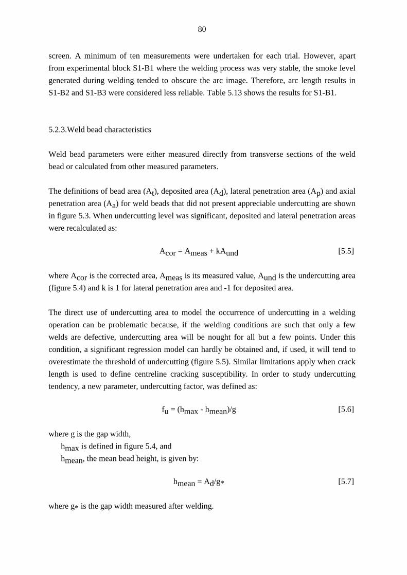
80
screen. A minimum of ten measurements were undertaken for each trial. However, apartfrom experimental block S1-B1 where the welding process was very stable, the smoke levelgenerated during welding tended to obscure the arc image. Therefore, arc length results inS1-B2 and S1-B3 were considered less reliable. Table 5.13 shows the results for S1-B1.
5.2.3.Weld bead characteristics
Weld bead parameters were either measured directly from transverse sections of the weldbead or calculated from other measured parameters.
The definitions of bead area (At), deposited area (Ad), lateral penetration area (Ap) and axialpenetration area (Aa) for weld beads that did not present appreciable undercutting are shownin figure 5.3. When undercutting level was significant, deposited and lateral penetration areaswere recalculated as:
Acor = Ameas + kAund [5.5]
where Acor is the corrected area, Ameas is its measured value, Aund is the undercutting area(figure 5.4) and k is 1 for lateral penetration area and -1 for deposited area.
The direct use of undercutting area to model the occurrence of undercutting in a weldingoperation can be problematic because, if the welding conditions are such that only a fewwelds are defective, undercutting area will be nought for all but a few points. Under thiscondition, a significant regression model can hardly be obtained and, if used, it will tend tooverestimate the threshold of undercutting (figure 5.5). Similar limitations apply when cracklength is used to define centreline cracking susceptibility. In order to study undercuttingtendency, a new parameter, undercutting factor, was defined as:
fu = (hmax - hmean)/g [5.6]
where g is the gap width, hmax is defined in figure 5.4, and hmean, the mean bead height, is given by:
hmean = Ad/g* [5.7]
where g* is the gap width measured after welding.
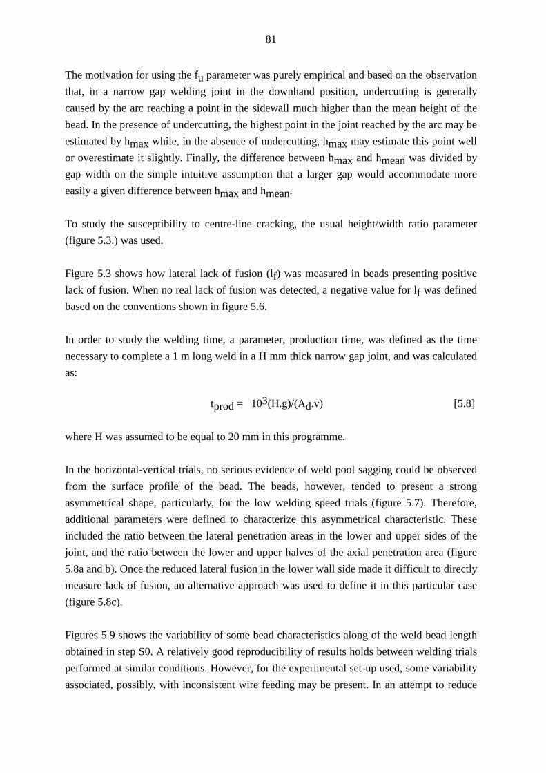
81
The motivation for using the fu parameter was purely empirical and based on the observationthat, in a narrow gap welding joint in the downhand position, undercutting is generallycaused by the arc reaching a point in the sidewall much higher than the mean height of thebead. In the presence of undercutting, the highest point in the joint reached by the arc may beestimated by hmax while, in the absence of undercutting, hmax may estimate this point wellor overestimate it slightly. Finally, the difference between hmax and hmean was divided bygap width on the simple intuitive assumption that a larger gap would accommodate moreeasily a given difference between hmax and hmean.
To study the susceptibility to centre-line cracking, the usual height/width ratio parameter(figure 5.3.) was used.
Figure 5.3 shows how lateral lack of fusion (lf) was measured in beads presenting positivelack of fusion. When no real lack of fusion was detected, a negative value for lf was definedbased on the conventions shown in figure 5.6.
In order to study the welding time, a parameter, production time, was defined as the timenecessary to complete a 1 m long weld in a H mm thick narrow gap joint, and was calculatedas:
tprod = 103(H.g)/(Ad.v) [5.8]
where H was assumed to be equal to 20 mm in this programme.
In the horizontal-vertical trials, no serious evidence of weld pool sagging could be observedfrom the surface profile of the bead. The beads, however, tended to present a strongasymmetrical shape, particularly, for the low welding speed trials (figure 5.7). Therefore,additional parameters were defined to characterize this asymmetrical characteristic. Theseincluded the ratio between the lateral penetration areas in the lower and upper sides of thejoint, and the ratio between the lower and upper halves of the axial penetration area (figure5.8a and b). Once the reduced lateral fusion in the lower wall side made it difficult to directlymeasure lack of fusion, an alternative approach was used to define it in this particular case(figure 5.8c).
Figures 5.9 shows the variability of some bead characteristics along of the weld bead lengthobtained in step S0. A relatively good reproducibility of results holds between welding trialsperformed at similar conditions. However, for the experimental set-up used, some variabilityassociated, possibly, with inconsistent wire feeding may be present. In an attempt to reduce
82
variability effects, bead parameters for each experimental trial were measured on threedifferent sections of the welded specimen.
The measured bead characteristics for all modelling experimental steps are shown in tables5.14-5.18.
5.2.4.Complementary trials
Table 5.19 presents the welding bead parameters of complementary trials of block S3-B1.The macrosection of the multipass downhand and horizontal-vertical specimens are shown infigure 5.10.
5.3.Modelling procedure
The experimental results of the previous sections were used for developing modellingequations for different aspects of the welding process, particularly, those related to the weldgeometry. The basic objective of modelling was to extract the useful part of the informationcontained in the experimental data and to summarize it in mathematical expressions foreasier interpretation and handling.
The basic tool used in this programme of data analysis and model building was multiplelinear regression. Different modelling formulations were attempted. The most commonlyused form was (MODEL A):
∑=
+=p
iiitrans xaay
10 [5.9]
where ytrans = yt (equation [2.35]) is a power transformation of the response y, xi's are p predictor variables from a initial set of k predictor candidates (k_p) that wereincluded in the model based on some criteria, and a0 and ai's are coefficients to be determined by multiple linear regression.
Transformation of the dependent variable was used to improve nonnormality, to reduceheterogeneous variance of errors and to accommodate non-linear trends in the model. Thisprocedure was preferred over adding second or higher order predictor interactions because itcan result in simpler models of easier interpretation. As these equations were to be used not
83
only for mapping the welding process response but also to provide a base for a betterunderstanding of its behaviour, simpler models were considered more desirable.
Adopting a model format such as equation [5.9] implies accepting that a linear relationshipexists between the predictor variables and some transformed form yt of the response. Such anassumption is obviously an oversimplification of the complex processes taking place inwelding. However, by investigating a relatively restricted region in the process operationalspace, one can expect that a linear model can provide a reasonably close description of thetrue unknown, and possibly not linear, relationship (figure 5.11).
The modelling procedure included the following steps:
. Transformation of the response using equation [2.35]. Values between -1 and 2,with intervals of 0.5, were generally used for the exponent t. For a nought value of t,a logarithmic transformation, ytrans = ln(y), was employed.
. Selection of the "best" set of predictors for ytrans. Usually, the initial set ofpredictor candidates included welding current, wire feed speed, welding speed andgap width. The selection of predictors was performed by backward elimination(§2.4.3.3). A significance level higher than 0.1 (the default value taken by theSPSSx programme) for the partial F ratios was used as the criterion to dropvariables from the model.
. Selection of the best transformation factor t for a given response y. Following theprocedure devised by Box and Cox (1964), the optimum t was considered thatwhich provided the minimum value for the mean square error (MSet) in the familyof transformations [2.37] (see §2.4.3.3). The 95% confidence interval on thetransformation factor t was obtained by calculating MSe* (equation [2.38]) andfinding the interception points between the MSe* horizontal line and the MSetcurve (figure 5.12). Residual plots and predicted value plots were carefullyexamined at this stage and possible outliers considered for exclusion from the datamatrix before a final value of t was accepted.
. Model diagnosis. In order to assess the model adequacy, residuals plot, predictedvalues plot and the statistics R2 and F ratio were considered. No rigid criteria wereset to define model adequacy. Generally, significance of F lower than about 0.001coupled with reasonable residual plots were considered sufficient. However, evenwhen the statistics of a given equation were not favourable, it could be considered
84
satisfactory for comparative analysis, when it showed a similar trend with similarequations of other experimental blocks.
Other alternative model forms that were also considered, included: (a)linear model withsecond order interactions (MODEL B)
∑∑−
>==
++=pp
ijijiij
p
iiitrans xxaxaay
,1
,110 [5.10]
and (b)logarithmic model (MODEL C):
( )∑=
+=p
iii xaay
10 ln)ln( [5.11]
Equation [5.10] was considered and used only when no satisfactory form of the basic model(equation [5.9]) could be fitted to a particular response.
Meanwhile, equation [5.11] was used as an alternative model form in those cases in which asimilar theoretical model could be developed based on the balance of mass between the metalfed by the wire and the resulting bead volume. If metal losses can be considered negligible,this relationship can be expressed as:
π (dw2/4)w = Ad.v [5.12]
or
Ad = [k'π (dw2/4)].w/v [5.13]
where k' can be a factor that depends on the units of measuring used. The theoreticalexpressions for mean bead height and production time can be easily derived from equations[5.7], [5.8] and [5.13]:
hmean = Ad/g* ≈ k'.w/(v.g), and [5.14]
tp = (103H/k').(g/w) [5.15]
Equations [5.13], [5.14] and [5.15] are readily transformed into the equation [5.11] format bytaking logarithms of both sides of each expression.
85
5.4.Modelling results
Graphs of R2, F ratio and corrected mean square error (MSet) against transformation factor(t) are presented in figures 5.13 to 5.16 for some of the studied responses. In most cases, the"best" transformation factor, which corresponded to a minimum for MSet, could be foundinside the (-1,2) interval. When it was located outside this interval, the outmost t value thatcorresponded to the smallest MSet was considered to be the "best" t. An "optimum"transformation factor that was common to as many experimental blocks as possible wasselected by comparing the 95% confidence intervals on t. Table 5.20 summarizes theinformation regarding transformation factors that was used to develop MODEL A typeequations (tables 5.21 and 5.22).
Predicted value plots for some responses of blocks S1-B1, S1-B2 and S2-B1 are shown infigures 5.17 to 5.19 for model A type equations. The points that were considered outliers andwere not included in the linear regression process are marked by the number of theirexperimental trial. Most of these points could be associated with some operational problemor with an welding condition that strongly affected the response considered. For instance,trials #1 and #14 in block S1-B2 presented serious control problems, probably associatedwith inconsistent wire feeding. Consequently, only a fraction of the resulting beads turnedout to be satisfactory and the validity of measurement could not be guaranteed. Hence, datafrom these trials were excluded from model building whenever the diagnosis stage providedan indication for that. Points #3 in S1-B1 and #2 in S1-B2 presented abnormally small axialpenetration areas in comparison with other trials and tended to influence strongly the Aaequation. Analysis of their macrosections and welding parameters indicated that, in one case,an excessively high wire feed rate associated with low current and welding speed in a verynarrow gap resulted in a thick liquid layer between the arc and base metal which may haveimpaired axial fusion. In the other trial, the arc seems to have deflected almost completely tothe sidewalls not reaching the bottom of the joint. These beads showed evidence of eitherhigh undercutting or lack of fusion levels and these would certainly prevent their use forproduction welding, and so it was decided to exclude their Aa values from modelling.Finally, many measured values from trial #18 of S2-B1 tended to stand clearly as an outlierin residuals plots. Although no apparent abnormality could be associated with this trial, thesedata were excluded from regression analysis based only on the results of model diagnosis.
Tables 5.23 and 5.24 present those cases in which a MODEL B type equation resulted insome improvement, in terms of R2 and significance of F ratio, when compared with previousequations.

86
MODEL C type equations do not appear to improve significantly on the previous results forAd, hmean, and tp (tables 5.25 and 5.26). However, their theoretical background is animportant advantage. These equations can be used, for instance, to check the validity of theexperimental conditions against the theoretical model.

87
Table 5.1 List of independent variable candidates without considering possiblerelationships among some of them.
Independent variable candidates
Welding current (I) Polarity (DC+/DC-) Current structure (if pulsed):
Peak current (Ip)Peak time (tp)Base current (Ib)Frequency (F)
Arc voltage (V) Power supply characteristics Wire feed speed (w) Wire diameter (dw) Wire composition Standoff distance (h) Electrode stickout (s) Arc length (la) Welding speed (v) Gap width (g)/other joint details Shielding gas composition Shielding gas flow rate (f) Welding position Torch/joint angle
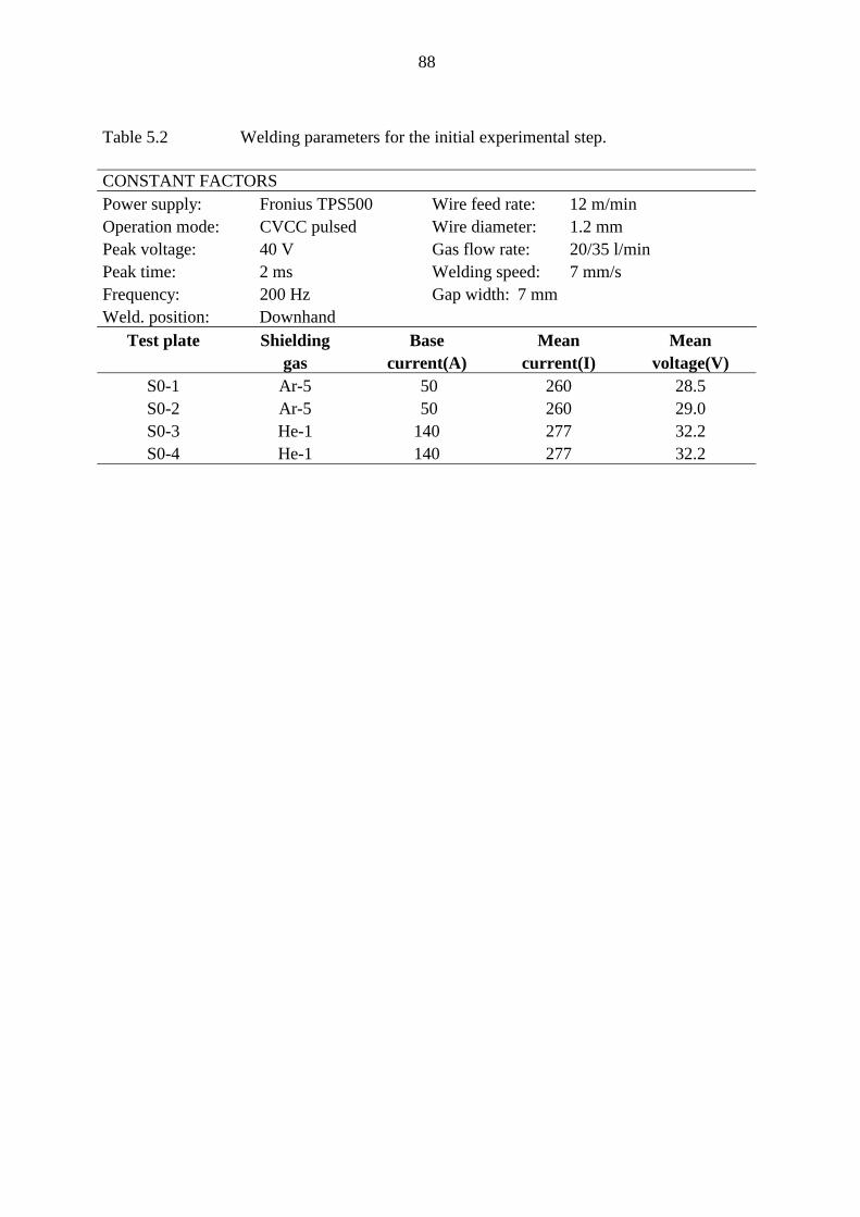
88
Table 5.2 Welding parameters for the initial experimental step.
CONSTANT FACTORSPower supply: Fronius TPS500Operation mode: CVCC pulsedPeak voltage: 40 VPeak time: 2 msFrequency: 200 HzWeld. position: Downhand
Wire feed rate: 12 m/minWire diameter: 1.2 mmGas flow rate: 20/35 l/minWelding speed: 7 mm/sGap width: 7 mm
Test plate Shieldinggas
Basecurrent(A)
Meancurrent(I)
Meanvoltage(V)
S0-1S0-2S0-3S0-4
Ar-5Ar-5He-1He-1
50 50140140
260260277277
28.529.032.232.2
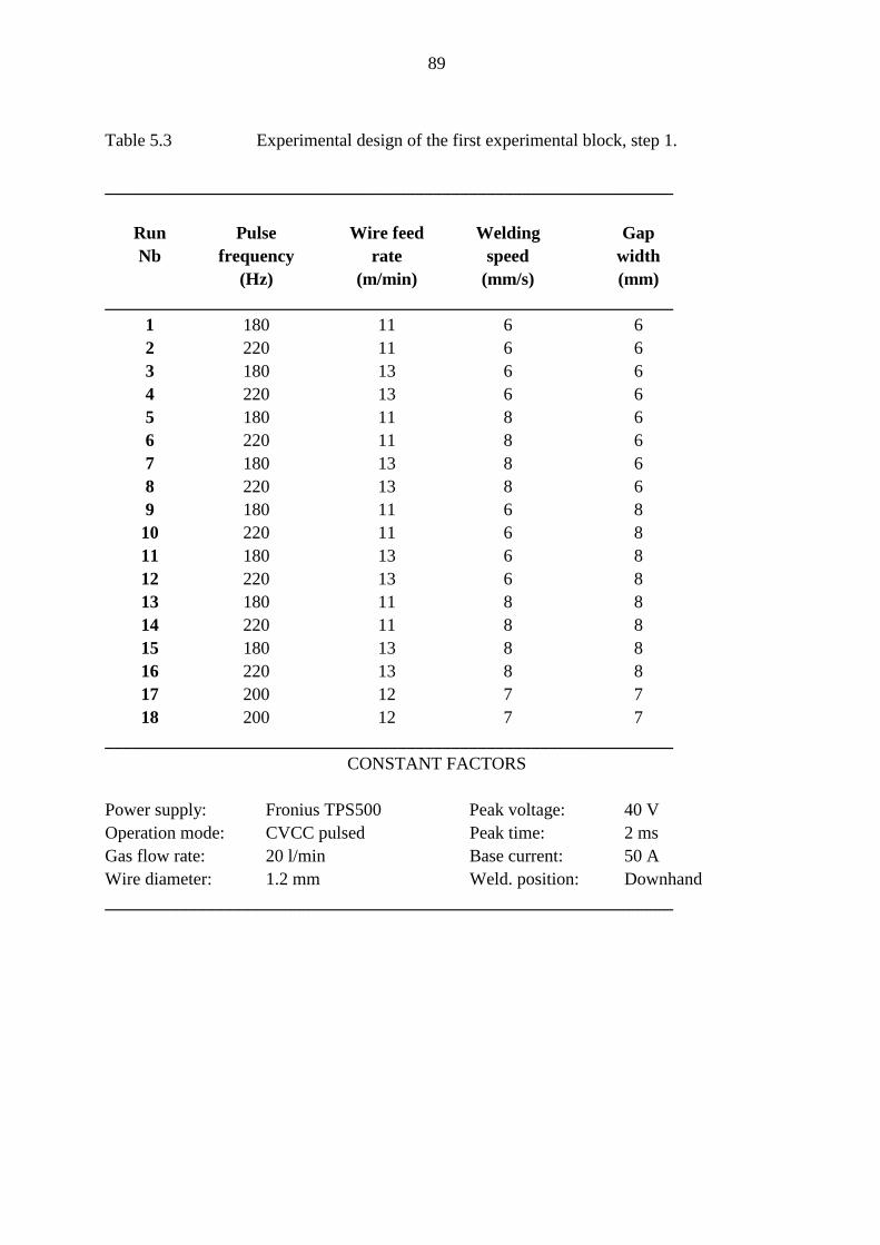
89
Table 5.3 Experimental design of the first experimental block, step 1.
________________________________________________________________
Run Pulse Wire feed Welding GapNb frequency rate speed width
(Hz) (m/min) (mm/s) (mm)________________________________________________________________
1 180 11 6 62 220 11 6 63 180 13 6 64 220 13 6 65 180 11 8 66 220 11 8 67 180 13 8 68 220 13 8 69 180 11 6 810 220 11 6 811 180 13 6 812 220 13 6 813 180 11 8 814 220 11 8 815 180 13 8 816 220 13 8 817 200 12 7 718 200 12 7 7
________________________________________________________________CONSTANT FACTORS
Power supply: Fronius TPS500 Peak voltage: 40 VOperation mode: CVCC pulsed Peak time: 2 msGas flow rate: 20 l/min Base current: 50 AWire diameter: 1.2 mm Weld. position: Downhand________________________________________________________________
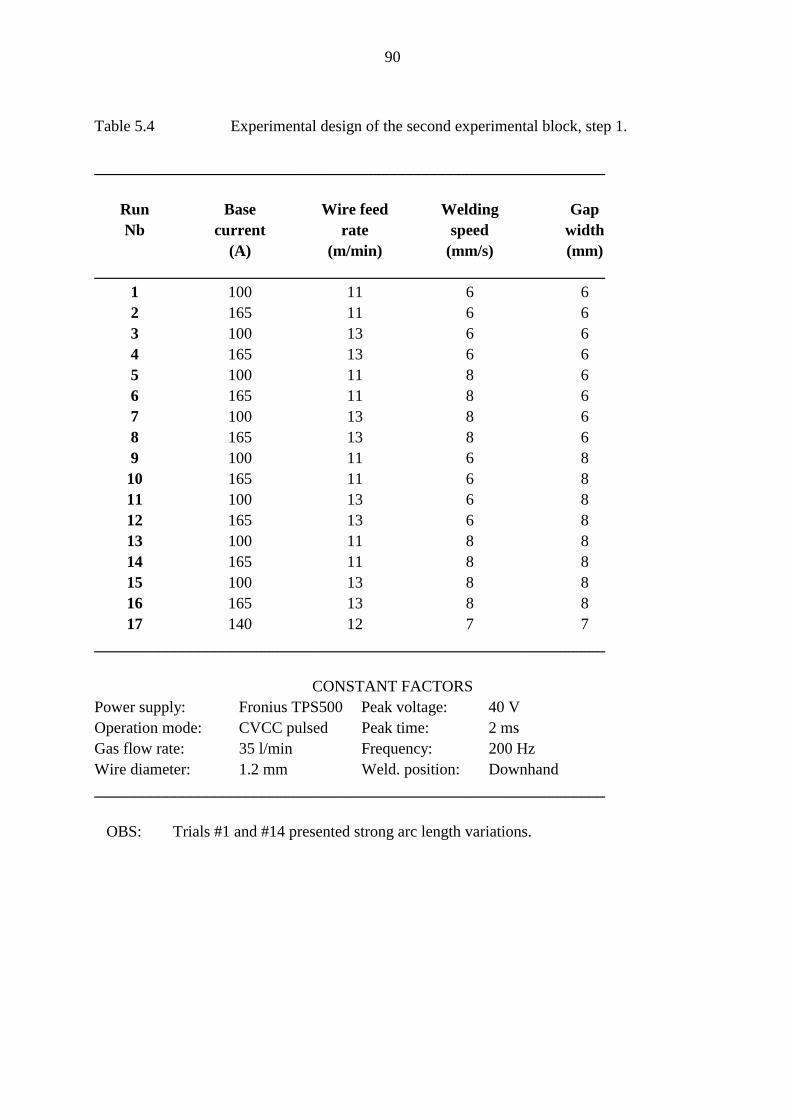
90
Table 5.4 Experimental design of the second experimental block, step 1.
________________________________________________________________
Run Base Wire feed Welding GapNb current rate speed width
(A) (m/min) (mm/s) (mm)________________________________________________________________
1 100 11 6 62 165 11 6 63 100 13 6 64 165 13 6 65 100 11 8 66 165 11 8 67 100 13 8 68 165 13 8 69 100 11 6 810 165 11 6 811 100 13 6 812 165 13 6 813 100 11 8 814 165 11 8 815 100 13 8 816 165 13 8 817 140 12 7 7
________________________________________________________________
CONSTANT FACTORSPower supply: Fronius TPS500 Peak voltage: 40 VOperation mode: CVCC pulsed Peak time: 2 msGas flow rate: 35 l/min Frequency: 200 HzWire diameter: 1.2 mm Weld. position: Downhand________________________________________________________________
OBS: Trials #1 and #14 presented strong arc length variations.
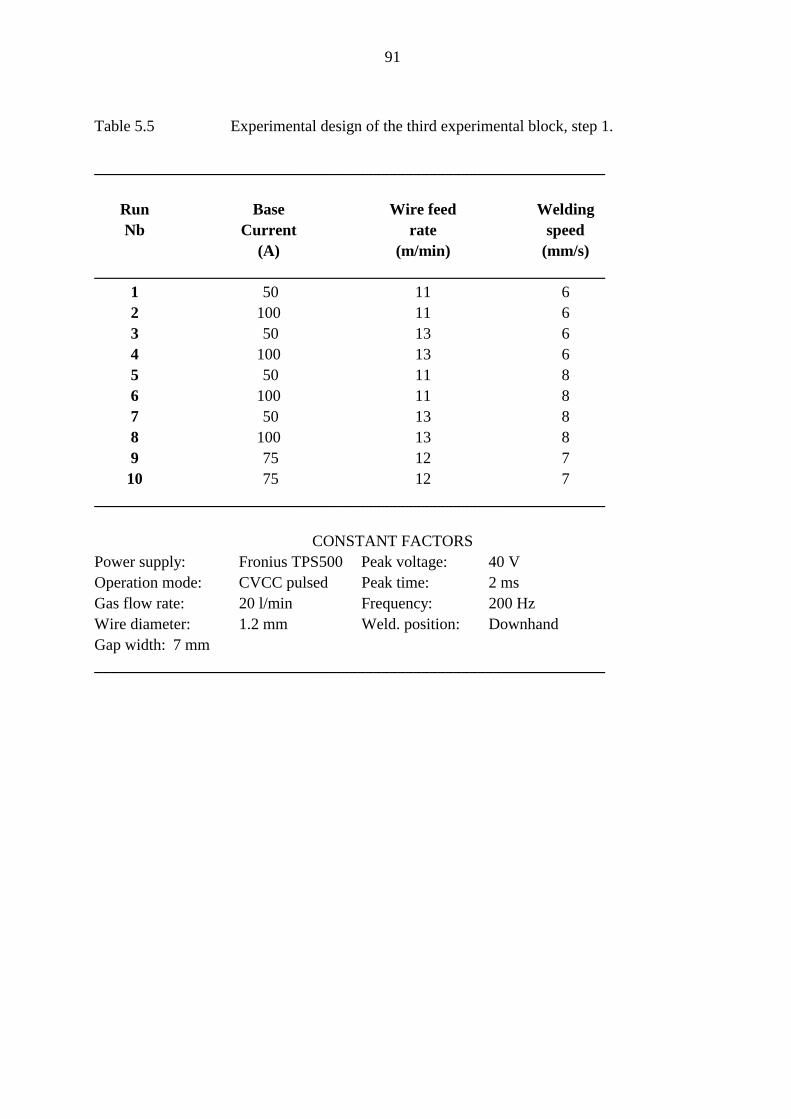
91
Table 5.5 Experimental design of the third experimental block, step 1.
________________________________________________________________
Run Base Wire feed WeldingNb Current rate speed
(A) (m/min) (mm/s)________________________________________________________________
1 50 11 62 100 11 63 50 13 64 100 13 65 50 11 86 100 11 87 50 13 88 100 13 89 75 12 710 75 12 7
________________________________________________________________
CONSTANT FACTORSPower supply: Fronius TPS500 Peak voltage: 40 VOperation mode: CVCC pulsed Peak time: 2 msGas flow rate: 20 l/min Frequency: 200 HzWire diameter: 1.2 mm Weld. position: DownhandGap width: 7 mm________________________________________________________________
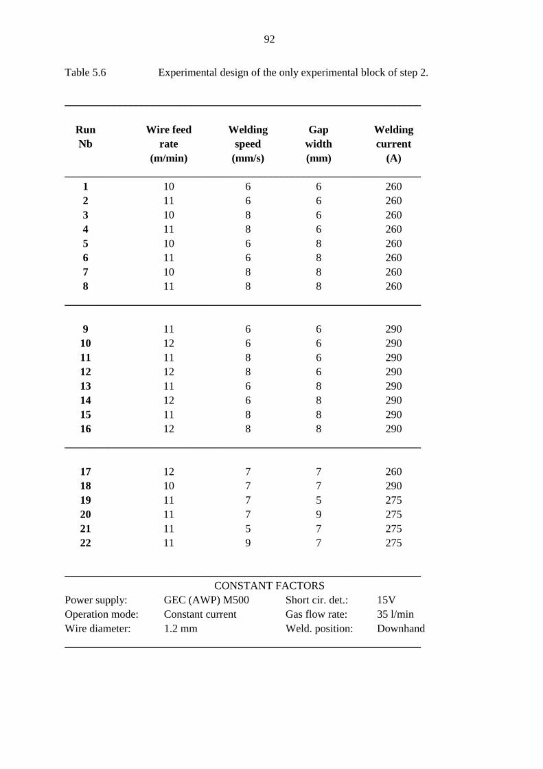
92
Table 5.6 Experimental design of the only experimental block of step 2.
_________________________________________________________________
Run Wire feed Welding Gap WeldingNb rate speed width current
(m/min) (mm/s) (mm) (A)_________________________________________________________________
1 10 6 6 2602 11 6 6 2603 10 8 6 2604 11 8 6 2605 10 6 8 2606 11 6 8 2607 10 8 8 2608 11 8 8 260
_________________________________________________________________
9 11 6 6 29010 12 6 6 29011 11 8 6 29012 12 8 6 29013 11 6 8 29014 12 6 8 29015 11 8 8 29016 12 8 8 290
_________________________________________________________________
17 12 7 7 26018 10 7 7 29019 11 7 5 27520 11 7 9 27521 11 5 7 27522 11 9 7 275
_________________________________________________________________CONSTANT FACTORS
Power supply: GEC (AWP) M500 Short cir. det.: 15VOperation mode: Constant current Gas flow rate: 35 l/minWire diameter: 1.2 mm Weld. position: Downhand_________________________________________________________________
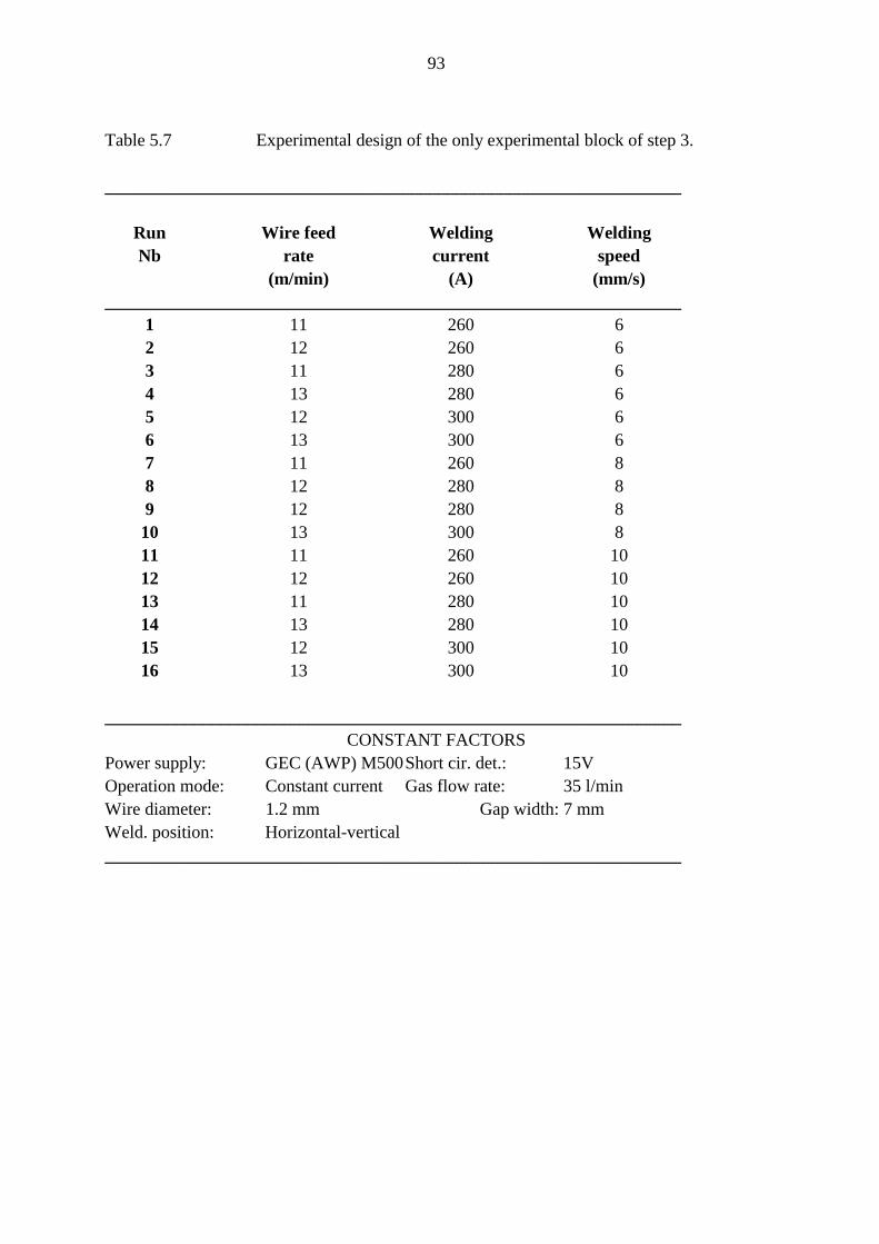
93
Table 5.7 Experimental design of the only experimental block of step 3.
_________________________________________________________________
Run Wire feed Welding WeldingNb rate current speed
(m/min) (A) (mm/s)_________________________________________________________________
1 11 260 62 12 260 63 11 280 64 13 280 65 12 300 66 13 300 67 11 260 88 12 280 89 12 280 810 13 300 811 11 260 1012 12 260 1013 11 280 1014 13 280 1015 12 300 1016 13 300 10
_________________________________________________________________CONSTANT FACTORS
Power supply: GEC (AWP) M500Short cir. det.: 15VOperation mode: Constant current Gas flow rate: 35 l/minWire diameter: 1.2 mm Gap width: 7 mmWeld. position: Horizontal-vertical_________________________________________________________________
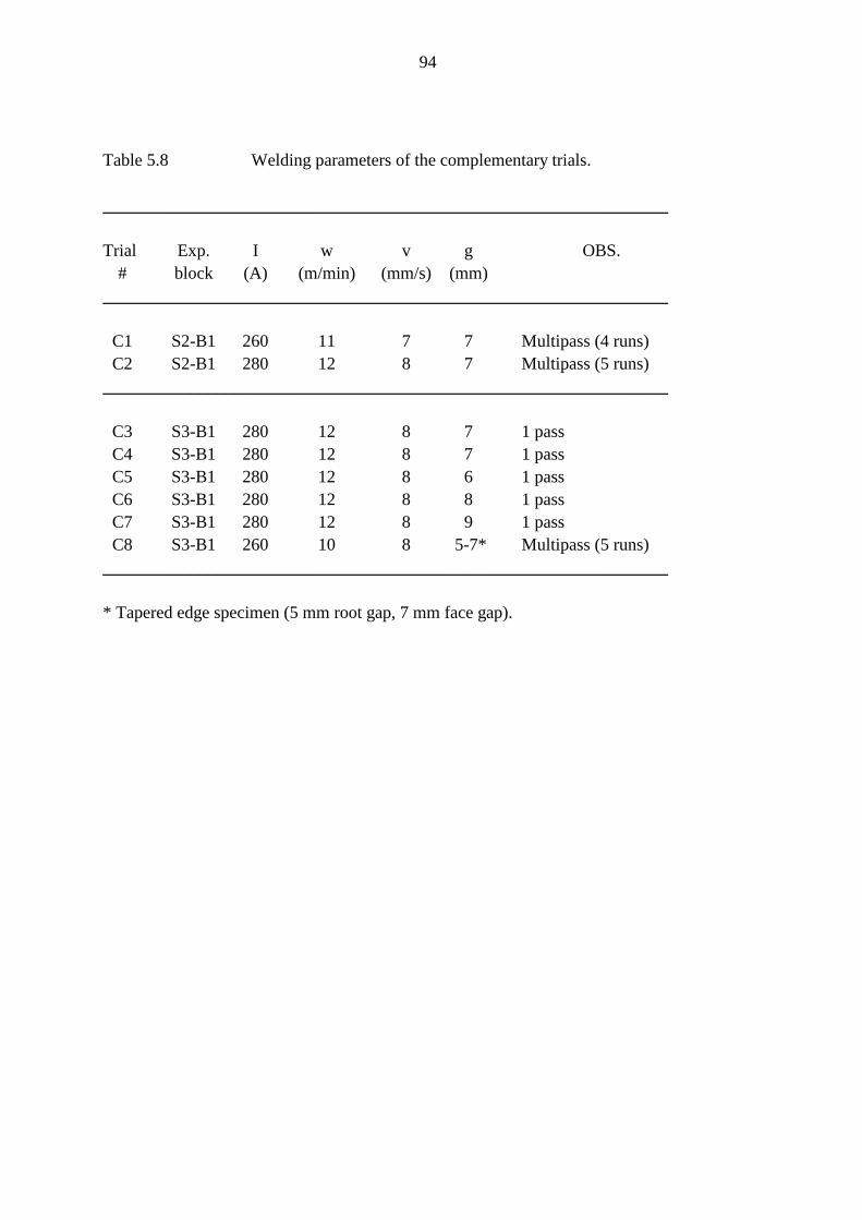
94
Table 5.8 Welding parameters of the complementary trials.
_________________________________________________________________
Trial Exp. I w v g OBS.# block (A) (m/min) (mm/s) (mm)
_________________________________________________________________
C1 S2-B1 260 11 7 7 Multipass (4 runs)C2 S2-B1 280 12 8 7 Multipass (5 runs)
_________________________________________________________________
C3 S3-B1 280 12 8 7 1 passC4 S3-B1 280 12 8 7 1 passC5 S3-B1 280 12 8 6 1 passC6 S3-B1 280 12 8 8 1 passC7 S3-B1 280 12 8 9 1 passC8 S3-B1 260 10 8 5-7* Multipass (5 runs)
_________________________________________________________________
* Tapered edge specimen (5 mm root gap, 7 mm face gap).

95
Table 5.9 List of measured parameters.
_________________________________________________________________
Dependent variables_________________________________________________________________
(a)Electrical parameters:. Mean current (I). Mean voltage (V). Pulse structure (pulsed welding):
. Peak current (Ip)
. Standard deviation of Ip (sp)
. Peak time (tp)
. Base current (Ib)
. Frequency (F)
(b)Arc parameters:. Arc length (la)
(c)Bead parameters:. Bead area (At). Deposited area (Ad). Lateral penetration area (Ap). Axial penetration area (Aa). Undercutting area (Aund). Lateral lack of fusion (lf). Maximum axial penetration (pa). Mean bead height (hmean). Centre-line crack length (lck). Gap contraction (dg). Height/width ratio (R). Undercutting factor (fu). Production time (tprod)
(d)Bead parameters (horizontal-vertical welding):. Upper side lateral penetration area (Apu). Lower side lateral penetration area (Apl). Apl/Apu ratio (Rplu). Upper axial penetration area (Aau). Lower axial penetration area (Aal). Aal/Aau ratio (Ralu)
_________________________________________________________________
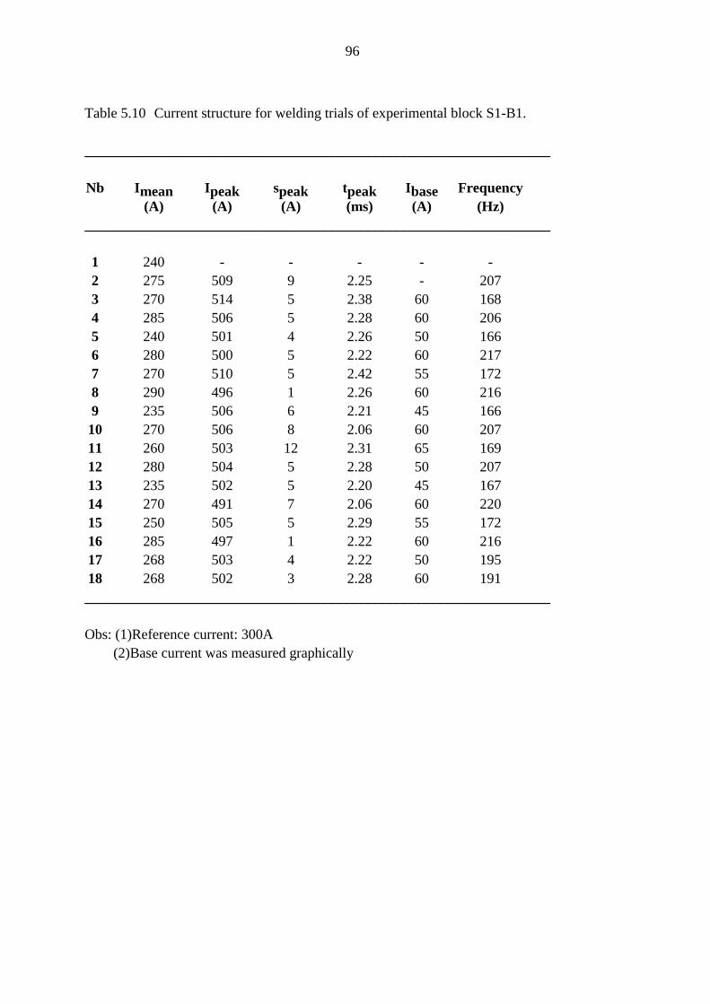
96
Table 5.10 Current structure for welding trials of experimental block S1-B1.
_________________________________________________________________
Nb Imean Ipeak speak tpeak Ibase Frequency(A) (A) (A) (ms) (A) (Hz)
_________________________________________________________________
1 240 - - - - -2 275 509 9 2.25 - 2073 270 514 5 2.38 60 1684 285 506 5 2.28 60 2065 240 501 4 2.26 50 1666 280 500 5 2.22 60 2177 270 510 5 2.42 55 1728 290 496 1 2.26 60 216
9 235 506 6 2.21 45 16610 270 506 8 2.06 60 20711 260 503 12 2.31 65 16912 280 504 5 2.28 50 20713 235 502 5 2.20 45 16714 270 491 7 2.06 60 22015 250 505 5 2.29 55 17216 285 497 1 2.22 60 21617 268 503 4 2.22 50 19518 268 502 3 2.28 60 191_________________________________________________________________
Obs: (1)Reference current: 300A (2)Base current was measured graphically
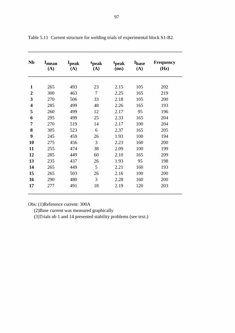
97
Table 5.11 Current structure for welding trials of experimental block S1-B2.
_________________________________________________________________
Nb Imean Ipeak speak tpeak Ibase Frequency(A) (A) (A) (ms) (A) (Hz)
_________________________________________________________________
1 265 493 23 2.15 105 2022 300 463 7 2.25 165 2193 270 506 33 2.18 105 2004 285 499 48 2.26 165 1935 260 499 12 2.17 95 1966 295 499 25 2.33 165 2047 270 519 14 2.17 100 2048 305 523 6 2.37 165 2059 245 459 26 1.93 100 19410 275 456 3 2.23 160 20011 255 474 38 2.09 100 19912 285 449 60 2.10 165 20913 235 437 26 1.93 95 19814 265 449 5 2.21 160 19315 265 503 26 2.16 100 20016 290 480 3 2.28 160 20017 277 491 18 2.19 120 203_________________________________________________________________
Obs: (1)Reference current: 300A (2)Base current was measured graphically (3)Trials nb 1 and 14 presented stability problems (see text.)
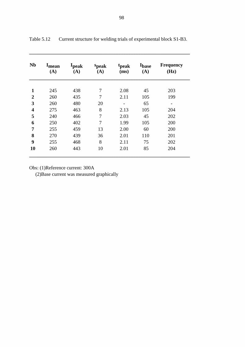
98
Table 5.12 Current structure for welding trials of experimental block S1-B3.
_________________________________________________________________
Nb Imean Ipeak speak tpeak Ibase Frequency(A) (A) (A) (ms) (A) (Hz)
_________________________________________________________________
1 245 438 7 2.08 45 2032 260 435 7 2.11 105 1993 260 480 20 - 65 -4 275 463 8 2.13 105 2045 240 466 7 2.03 45 2026 250 402 7 1.99 105 2007 255 459 13 2.00 60 2008 270 439 36 2.01 110 2019 255 468 8 2.11 75 20210 260 443 10 2.01 85 204_________________________________________________________________
Obs: (1)Reference current: 300A (2)Base current was measured graphically

99
Table 5.13 Arc length measurements for the experimental block S1-B1.
______________________________________________________________Nb Arc Standard Number of
length deviation measurements(mm) (mm)
______________________________________________________________
1 2.7 0.6 302 4.5 1.8 153 1.2 0.8 164 3.2 0.4 275 2.0 0.4 276 6.5 0.5 167 1.7 0.7 358 2.8 0.2 149 2.3 0.5 4310 3.2 0.3 2611 1.3 0.4 4112 1.9 0.2 2313 2.1 0.3 2814 4.0 0.3 2115 1.3 0.3 2416 2.1 0.2 1717 2.3 0.2 1918 2.1 0.3 16
______________________________________________________________
Mean: 2.6St. deviation: 1.3
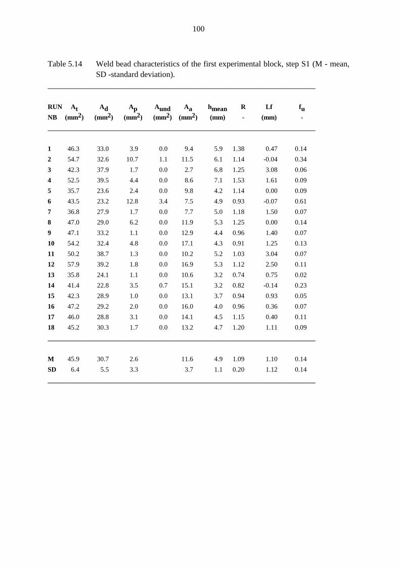
100
Table 5.14 Weld bead characteristics of the first experimental block, step S1 (M - mean,SD -standard deviation).
_______________________________________________________________________________
RUN At Ad Ap Aund Aa hmean R Lf fuNB (mm2) (mm2) (mm2) (mm2) (mm2) (mm) - (mm) -_______________________________________________________________________________
1 46.3 33.0 3.9 0.0 9.4 5.9 1.38 0.47 0.142 54.7 32.6 10.7 1.1 11.5 6.1 1.14 -0.04 0.343 42.3 37.9 1.7 0.0 2.7 6.8 1.25 3.08 0.064 52.5 39.5 4.4 0.0 8.6 7.1 1.53 1.61 0.095 35.7 23.6 2.4 0.0 9.8 4.2 1.14 0.00 0.096 43.5 23.2 12.8 3.4 7.5 4.9 0.93 -0.07 0.617 36.8 27.9 1.7 0.0 7.7 5.0 1.18 1.50 0.078 47.0 29.0 6.2 0.0 11.9 5.3 1.25 0.00 0.149 47.1 33.2 1.1 0.0 12.9 4.4 0.96 1.40 0.0710 54.2 32.4 4.8 0.0 17.1 4.3 0.91 1.25 0.1311 50.2 38.7 1.3 0.0 10.2 5.2 1.03 3.04 0.0712 57.9 39.2 1.8 0.0 16.9 5.3 1.12 2.50 0.1113 35.8 24.1 1.1 0.0 10.6 3.2 0.74 0.75 0.0214 41.4 22.8 3.5 0.7 15.1 3.2 0.82 -0.14 0.2315 42.3 28.9 1.0 0.0 13.1 3.7 0.94 0.93 0.0516 47.2 29.2 2.0 0.0 16.0 4.0 0.96 0.36 0.0717 46.0 28.8 3.1 0.0 14.1 4.5 1.15 0.40 0.1118 45.2 30.3 1.7 0.0 13.2 4.7 1.20 1.11 0.09_______________________________________________________________________________
M 45.9 30.7 2.6 11.6 4.9 1.09 1.10 0.14SD 6.4 5.5 3.3 3.7 1.1 0.20 1.12 0.14_______________________________________________________________________________
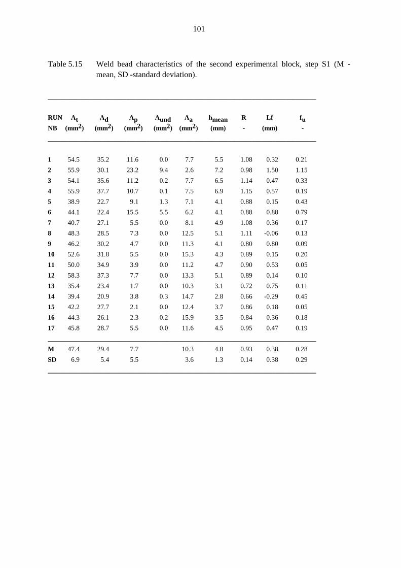
101
Table 5.15 Weld bead characteristics of the second experimental block, step S1 (M -mean, SD -standard deviation).
_______________________________________________________________________________
RUN At Ad Ap Aund Aa hmean R Lf fuNB (mm2) (mm2) (mm2) (mm2) (mm2) (mm) - (mm) -_______________________________________________________________________________
1 54.5 35.2 11.6 0.0 7.7 5.5 1.08 0.32 0.212 55.9 30.1 23.2 9.4 2.6 7.2 0.98 1.50 1.153 54.1 35.6 11.2 0.2 7.7 6.5 1.14 0.47 0.334 55.9 37.7 10.7 0.1 7.5 6.9 1.15 0.57 0.195 38.9 22.7 9.1 1.3 7.1 4.1 0.88 0.15 0.436 44.1 22.4 15.5 5.5 6.2 4.1 0.88 0.88 0.797 40.7 27.1 5.5 0.0 8.1 4.9 1.08 0.36 0.178 48.3 28.5 7.3 0.0 12.5 5.1 1.11 -0.06 0.139 46.2 30.2 4.7 0.0 11.3 4.1 0.80 0.80 0.0910 52.6 31.8 5.5 0.0 15.3 4.3 0.89 0.15 0.2011 50.0 34.9 3.9 0.0 11.2 4.7 0.90 0.53 0.0512 58.3 37.3 7.7 0.0 13.3 5.1 0.89 0.14 0.1013 35.4 23.4 1.7 0.0 10.3 3.1 0.72 0.75 0.1114 39.4 20.9 3.8 0.3 14.7 2.8 0.66 -0.29 0.4515 42.2 27.7 2.1 0.0 12.4 3.7 0.86 0.18 0.0516 44.3 26.1 2.3 0.2 15.9 3.5 0.84 0.36 0.1817 45.8 28.7 5.5 0.0 11.6 4.5 0.95 0.47 0.19_______________________________________________________________________________M 47.4 29.4 7.7 10.3 4.8 0.93 0.38 0.28SD 6.9 5.4 5.5 3.6 1.3 0.14 0.38 0.29_______________________________________________________________________________
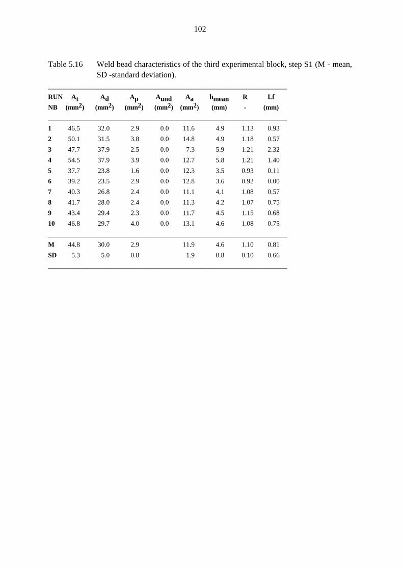
102
Table 5.16 Weld bead characteristics of the third experimental block, step S1 (M - mean,SD -standard deviation).
______________________________________________________________________RUN At Ad Ap Aund Aa hmean R LfNB (mm2) (mm2) (mm2) (mm2) (mm2) (mm) - (mm)______________________________________________________________________1 46.5 32.0 2.9 0.0 11.6 4.9 1.13 0.932 50.1 31.5 3.8 0.0 14.8 4.9 1.18 0.573 47.7 37.9 2.5 0.0 7.3 5.9 1.21 2.324 54.5 37.9 3.9 0.0 12.7 5.8 1.21 1.405 37.7 23.8 1.6 0.0 12.3 3.5 0.93 0.116 39.2 23.5 2.9 0.0 12.8 3.6 0.92 0.007 40.3 26.8 2.4 0.0 11.1 4.1 1.08 0.578 41.7 28.0 2.4 0.0 11.3 4.2 1.07 0.759 43.4 29.4 2.3 0.0 11.7 4.5 1.15 0.6810 46.8 29.7 4.0 0.0 13.1 4.6 1.08 0.75______________________________________________________________________M 44.8 30.0 2.9 11.9 4.6 1.10 0.81SD 5.3 5.0 0.8 1.9 0.8 0.10 0.66______________________________________________________________________
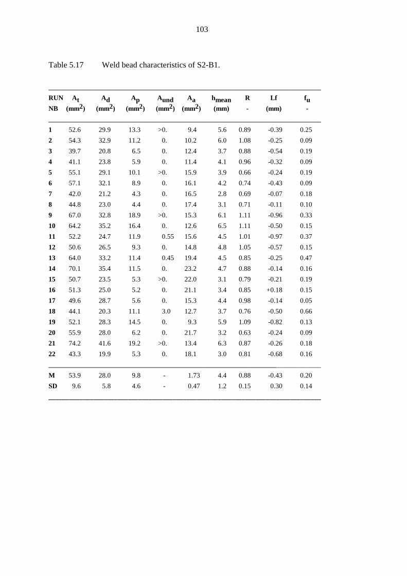
103
Table 5.17 Weld bead characteristics of S2-B1.
_______________________________________________________________________________RUN At Ad Ap Aund Aa hmean R Lf fuNB (mm2) (mm2) (mm2) (mm2) (mm2) (mm) - (mm) -_______________________________________________________________________________1 52.6 29.9 13.3 >0. 9.4 5.6 0.89 -0.39 0.252 54.3 32.9 11.2 0. 10.2 6.0 1.08 -0.25 0.093 39.7 20.8 6.5 0. 12.4 3.7 0.88 -0.54 0.194 41.1 23.8 5.9 0. 11.4 4.1 0.96 -0.32 0.095 55.1 29.1 10.1 >0. 15.9 3.9 0.66 -0.24 0.196 57.1 32.1 8.9 0. 16.1 4.2 0.74 -0.43 0.097 42.0 21.2 4.3 0. 16.5 2.8 0.69 -0.07 0.188 44.8 23.0 4.4 0. 17.4 3.1 0.71 -0.11 0.109 67.0 32.8 18.9 >0. 15.3 6.1 1.11 -0.96 0.3310 64.2 35.2 16.4 0. 12.6 6.5 1.11 -0.50 0.1511 52.2 24.7 11.9 0.55 15.6 4.5 1.01 -0.97 0.3712 50.6 26.5 9.3 0. 14.8 4.8 1.05 -0.57 0.1513 64.0 33.2 11.4 0.45 19.4 4.5 0.85 -0.25 0.4714 70.1 35.4 11.5 0. 23.2 4.7 0.88 -0.14 0.1615 50.7 23.5 5.3 >0. 22.0 3.1 0.79 -0.21 0.1916 51.3 25.0 5.2 0. 21.1 3.4 0.85 +0.18 0.1517 49.6 28.7 5.6 0. 15.3 4.4 0.98 -0.14 0.0518 44.1 20.3 11.1 3.0 12.7 3.7 0.76 -0.50 0.6619 52.1 28.3 14.5 0. 9.3 5.9 1.09 -0.82 0.1320 55.9 28.0 6.2 0. 21.7 3.2 0.63 -0.24 0.0921 74.2 41.6 19.2 >0. 13.4 6.3 0.87 -0.26 0.1822 43.3 19.9 5.3 0. 18.1 3.0 0.81 -0.68 0.16_______________________________________________________________________________M 53.9 28.0 9.8 - 1.73 4.4 0.88 -0.43 0.20SD 9.6 5.8 4.6 - 0.47 1.2 0.15 0.30 0.14_______________________________________________________________________________
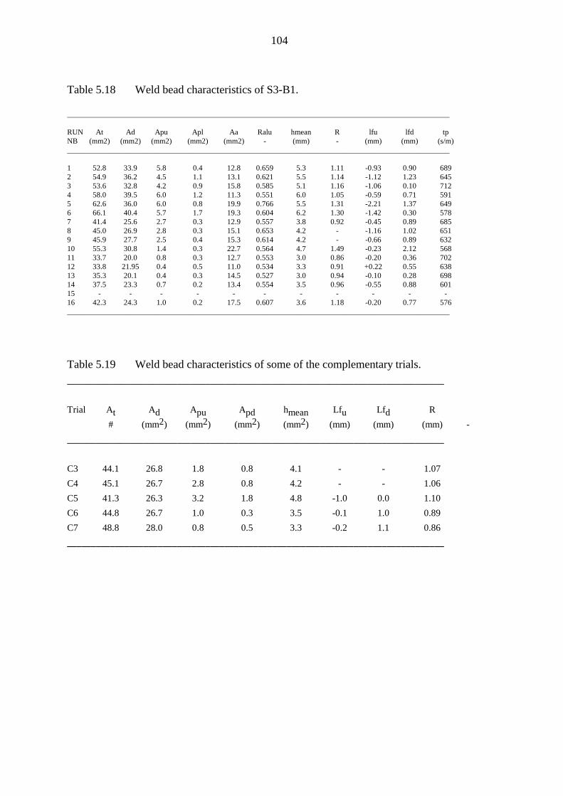
104
Table 5.18 Weld bead characteristics of S3-B1.
___________________________________________________________________________________________________
RUN At Ad Apu Apl Aa Ralu hmean R lfu lfd tpNB (mm2) (mm2) (mm2) (mm2) (mm2) - (mm) - (mm) (mm) (s/m)___________________________________________________________________________________________________
1 52.8 33.9 5.8 0.4 12.8 0.659 5.3 1.11 -0.93 0.90 6892 54.9 36.2 4.5 1.1 13.1 0.621 5.5 1.14 -1.12 1.23 6453 53.6 32.8 4.2 0.9 15.8 0.585 5.1 1.16 -1.06 0.10 7124 58.0 39.5 6.0 1.2 11.3 0.551 6.0 1.05 -0.59 0.71 5915 62.6 36.0 6.0 0.8 19.9 0.766 5.5 1.31 -2.21 1.37 6496 66.1 40.4 5.7 1.7 19.3 0.604 6.2 1.30 -1.42 0.30 5787 41.4 25.6 2.7 0.3 12.9 0.557 3.8 0.92 -0.45 0.89 6858 45.0 26.9 2.8 0.3 15.1 0.653 4.2 - -1.16 1.02 6519 45.9 27.7 2.5 0.4 15.3 0.614 4.2 - -0.66 0.89 63210 55.3 30.8 1.4 0.3 22.7 0.564 4.7 1.49 -0.23 2.12 56811 33.7 20.0 0.8 0.3 12.7 0.553 3.0 0.86 -0.20 0.36 70212 33.8 21.95 0.4 0.5 11.0 0.534 3.3 0.91 +0.22 0.55 63813 35.3 20.1 0.4 0.3 14.5 0.527 3.0 0.94 -0.10 0.28 69814 37.5 23.3 0.7 0.2 13.4 0.554 3.5 0.96 -0.55 0.88 60115 - - - - - - - - - - -16 42.3 24.3 1.0 0.2 17.5 0.607 3.6 1.18 -0.20 0.77 576___________________________________________________________________________________________________
Table 5.19 Weld bead characteristics of some of the complementary trials._______________________________________________________________________________
Trial At Ad Apu Apd hmean Lfu Lfd R# (mm2) (mm2) (mm2) (mm2) (mm) (mm) (mm) -
_______________________________________________________________________________
C3 44.1 26.8 1.8 0.8 4.1 - - 1.07C4 45.1 26.7 2.8 0.8 4.2 - - 1.06C5 41.3 26.3 3.2 1.8 4.8 -1.0 0.0 1.10C6 44.8 26.7 1.0 0.3 3.5 -0.1 1.0 0.89C7 48.8 28.0 0.8 0.5 3.3 -0.2 1.1 0.86_______________________________________________________________________________
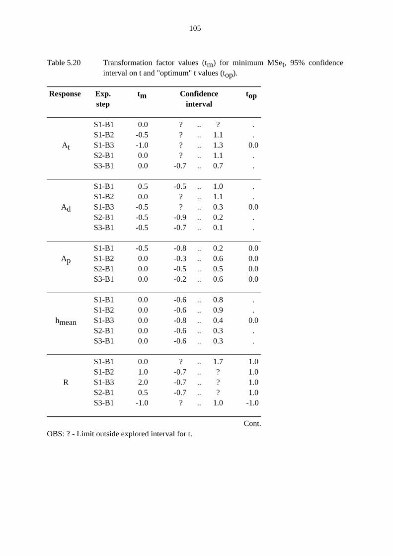
105
Table 5.20 Transformation factor values (tm) for minimum MSet, 95% confidenceinterval on t and "optimum" t values (top).
______________________________________________________Response Exp. tm Confidence top
step interval______________________________________________________
S1-B1 0.0 ? .. ? .S1-B2 -0.5 ? .. 1.1 .
At S1-B3 -1.0 ? .. 1.3 0.0S2-B1 0.0 ? .. 1.1 .S3-B1 0.0 -0.7 .. 0.7 .
______________________________________________________S1-B1 0.5 -0.5 .. 1.0 .S1-B2 0.0 ? .. 1.1 .
Ad S1-B3 -0.5 ? .. 0.3 0.0S2-B1 -0.5 -0.9 .. 0.2 .S3-B1 -0.5 -0.7 .. 0.1 .
______________________________________________________S1-B1 -0.5 -0.8 .. 0.2 0.0
Ap S1-B2 0.0 -0.3 .. 0.6 0.0S2-B1 0.0 -0.5 .. 0.5 0.0S3-B1 0.0 -0.2 .. 0.6 0.0
______________________________________________________S1-B1 0.0 -0.6 .. 0.8 .S1-B2 0.0 -0.6 .. 0.9 .
hmean S1-B3 0.0 -0.8 .. 0.4 0.0S2-B1 0.0 -0.6 .. 0.3 .S3-B1 0.0 -0.6 .. 0.3 .
______________________________________________________S1-B1 0.0 ? .. 1.7 1.0S1-B2 1.0 -0.7 .. ? 1.0
R S1-B3 2.0 -0.7 .. ? 1.0S2-B1 0.5 -0.7 .. ? 1.0S3-B1 -1.0 ? .. 1.0 -1.0
______________________________________________________Cont.
OBS: ? - Limit outside explored interval for t.
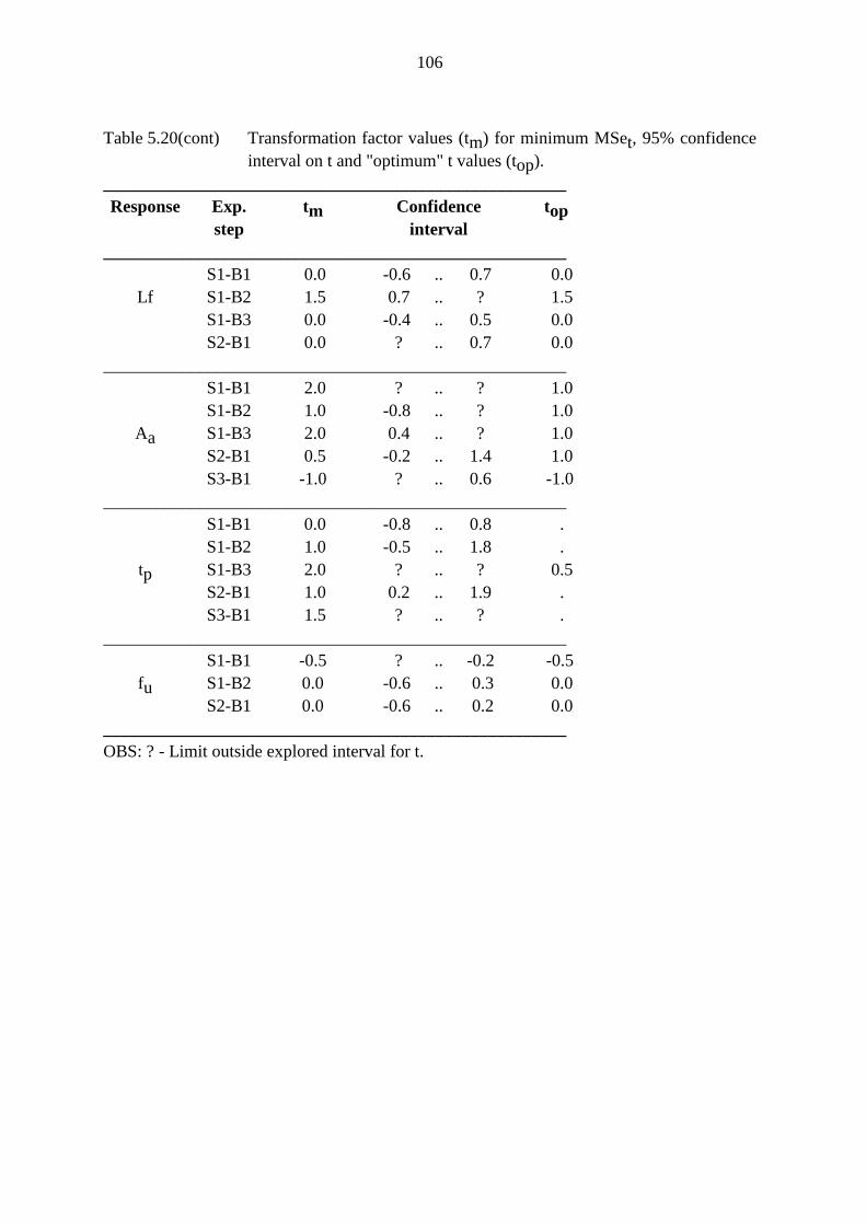
106
Table 5.20(cont) Transformation factor values (tm) for minimum MSet, 95% confidenceinterval on t and "optimum" t values (top).
_____________________________________________________Response Exp. tm Confidence top
step interval_____________________________________________________
S1-B1 0.0 -0.6 .. 0.7 0.0Lf S1-B2 1.5 0.7 .. ? 1.5
S1-B3 0.0 -0.4 .. 0.5 0.0S2-B1 0.0 ? .. 0.7 0.0
_____________________________________________________S1-B1 2.0 ? .. ? 1.0S1-B2 1.0 -0.8 .. ? 1.0
Aa S1-B3 2.0 0.4 .. ? 1.0S2-B1 0.5 -0.2 .. 1.4 1.0S3-B1 -1.0 ? .. 0.6 -1.0
_____________________________________________________S1-B1 0.0 -0.8 .. 0.8 .S1-B2 1.0 -0.5 .. 1.8 .
tp S1-B3 2.0 ? .. ? 0.5S2-B1 1.0 0.2 .. 1.9 .S3-B1 1.5 ? .. ? .
_____________________________________________________S1-B1 -0.5 ? .. -0.2 -0.5
fu S1-B2 0.0 -0.6 .. 0.3 0.0S2-B1 0.0 -0.6 .. 0.2 0.0
_____________________________________________________OBS: ? - Limit outside explored interval for t.
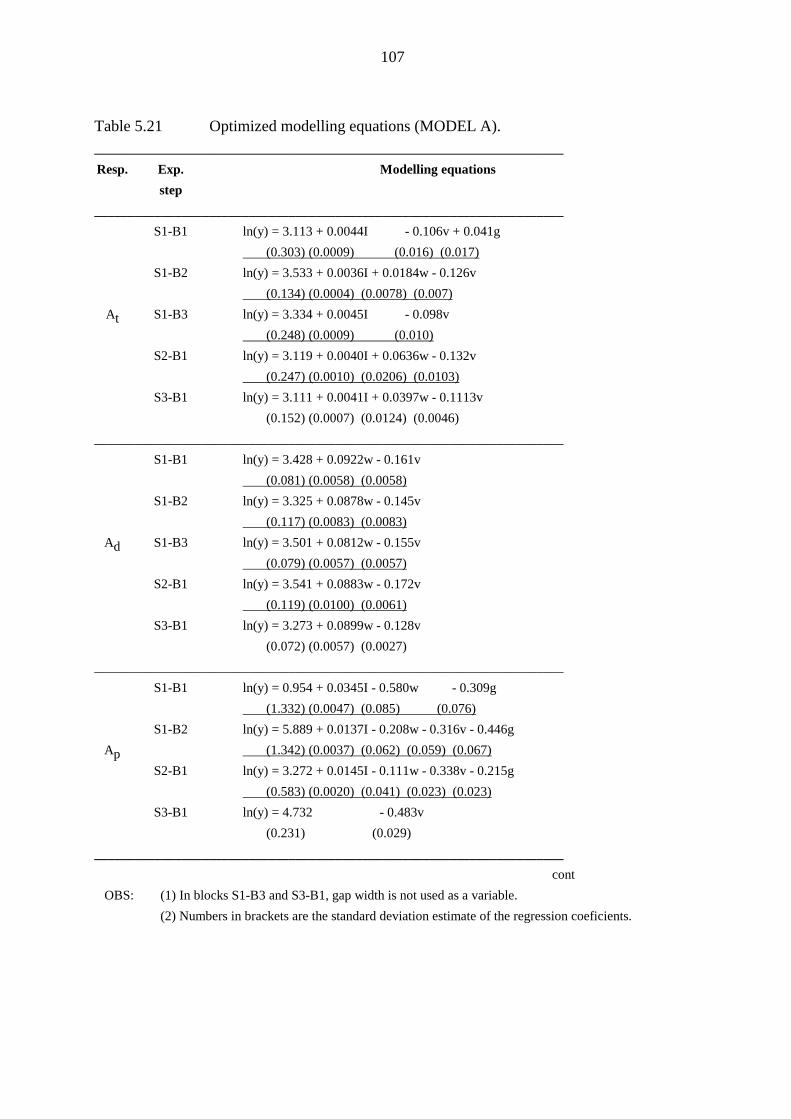
107
Table 5.21 Optimized modelling equations (MODEL A).______________________________________________________________________Resp. Exp. Modelling equations
step______________________________________________________________________
S1-B1 ln(y) = 3.113 + 0.0044I - 0.106v + 0.041g (0.303) (0.0009) (0.016) (0.017)
S1-B2 ln(y) = 3.533 + 0.0036I + 0.0184w - 0.126v (0.134) (0.0004) (0.0078) (0.007)
At S1-B3 ln(y) = 3.334 + 0.0045I - 0.098v (0.248) (0.0009) (0.010)
S2-B1 ln(y) = 3.119 + 0.0040I + 0.0636w - 0.132v (0.247) (0.0010) (0.0206) (0.0103)
S3-B1 ln(y) = 3.111 + 0.0041I + 0.0397w - 0.1113v (0.152) (0.0007) (0.0124) (0.0046)
______________________________________________________________________S1-B1 ln(y) = 3.428 + 0.0922w - 0.161v
(0.081) (0.0058) (0.0058)S1-B2 ln(y) = 3.325 + 0.0878w - 0.145v
(0.117) (0.0083) (0.0083)Ad S1-B3 ln(y) = 3.501 + 0.0812w - 0.155v
(0.079) (0.0057) (0.0057)S2-B1 ln(y) = 3.541 + 0.0883w - 0.172v
(0.119) (0.0100) (0.0061)S3-B1 ln(y) = 3.273 + 0.0899w - 0.128v
(0.072) (0.0057) (0.0027)______________________________________________________________________
S1-B1 ln(y) = 0.954 + 0.0345I - 0.580w - 0.309g (1.332) (0.0047) (0.085) (0.076)
S1-B2 ln(y) = 5.889 + 0.0137I - 0.208w - 0.316v - 0.446gAp (1.342) (0.0037) (0.062) (0.059) (0.067)
S2-B1 ln(y) = 3.272 + 0.0145I - 0.111w - 0.338v - 0.215g (0.583) (0.0020) (0.041) (0.023) (0.023)
S3-B1 ln(y) = 4.732 - 0.483v (0.231) (0.029)
______________________________________________________________________cont
OBS: (1) In blocks S1-B3 and S3-B1, gap width is not used as a variable.(2) Numbers in brackets are the standard deviation estimate of the regression coeficients.
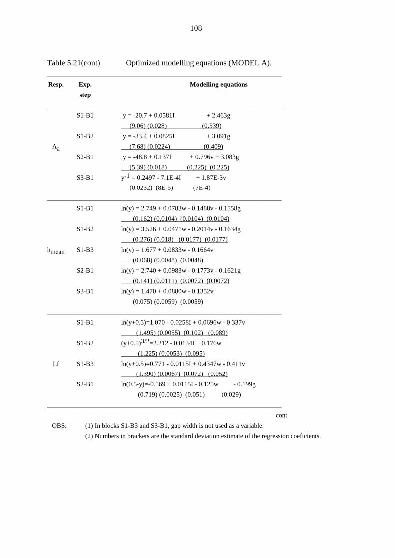
108
Table 5.21(cont) Optimized modelling equations (MODEL A).______________________________________________________________________Resp. Exp. Modelling equations
step______________________________________________________________________
S1-B1 y = -20.7 + 0.0581I + 2.463g (9.06) (0.028) (0.539)
S1-B2 y = -33.4 + 0.0825I + 3.091gAa (7.68) (0.0224) (0.409)
S2-B1 y = -48.8 + 0.137I + 0.796v + 3.083g (5.39) (0.018) (0.225) (0.225)
S3-B1 y-1 = 0.2497 - 7.1E-4I + 1.87E-3v (0.0232) (8E-5) (7E-4)
______________________________________________________________________S1-B1 ln(y) = 2.749 + 0.0783w - 0.1488v - 0.1558g
(0.162) (0.0104) (0.0104) (0.0104)S1-B2 ln(y) = 3.526 + 0.0471w - 0.2014v - 0.1634g
(0.276) (0.018) (0.0177) (0.0177)hmean S1-B3 ln(y) = 1.677 + 0.0833w - 0.1664v
(0.068) (0.0048) (0.0048)S2-B1 ln(y) = 2.740 + 0.0983w - 0.1773v - 0.1621g
(0.141) (0.0111) (0.0072) (0.0072)S3-B1 ln(y) = 1.470 + 0.0880w - 0.1352v
(0.075) (0.0059) (0.0059)______________________________________________________________________
S1-B1 ln(y+0.5)=1.070 - 0.0258I + 0.0696w - 0.337v (1.495) (0.0055) (0.102) (0.089)
S1-B2 (y+0.5)3/2=2.212 - 0.0134I + 0.176w (1.225) (0.0053) (0.095)
Lf S1-B3 ln(y+0.5)=0.771 - 0.0115I + 0.4347w - 0.411v (1.390) (0.0067) (0.072) (0.052)
S2-B1 ln(0.5-y)=-0.569 + 0.0115I - 0.125w - 0.199g (0.719) (0.0025) (0.051) (0.029)
______________________________________________________________________cont
OBS: (1) In blocks S1-B3 and S3-B1, gap width is not used as a variable.(2) Numbers in brackets are the standard deviation estimate of the regression coeficients.
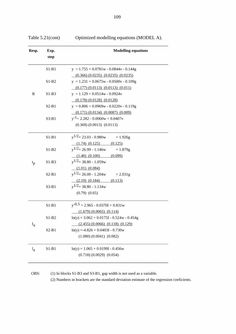
109
Table 5.21(cont) Optimized modelling equations (MODEL A).______________________________________________________________________Resp. Exp. Modelling equations
step______________________________________________________________________
S1-B1 y = 1.755 + 0.0781w - 0.0844v - 0.144g (0.366) (0.0235) (0.0235) (0.0235)
S1-B2 y = 1.231 + 0.0675w - 0.0500v - 0.109g (0.177) (0.0113) (0.0113) (0.011)
R S1-B3 y = 1.129 + 0.0514w - 0.0924v (0.178) (0.0128) (0.0128)
S2-B1 y = 0.806 + 0.0969w - 0.0220v - 0.119g (0.171) (0.0134) (0.0087) (0.009)
S3-B1 y-1= 2.282 - 0.0060w + 0.0407v (0.369) (0.0013) (0.0113)
______________________________________________________________________S1-B1 y1/2= 23.03 - 0.980w + 1.926g
(1.74) (0.125) (0.125)S1-B2 y1/2= 26.99 - 1.146w + 1.879g
(1.40) (0.100) (0.099)tp S1-B3 y1/2= 38.80 - 1.059w
(1.01) (0.084)S2-B1 y1/2= 26.00 - 1.204w + 2.031g
(2.19) (0.184) (0.113)S3-B1 y1/2= 38.80 - 1.134w
(0.79) (0.65)______________________________________________________________________
S1-B1 y-0.5 = 2.965 - 0.0370I + 0.831w (1.679) (0.0065) (0.114)
S1-B2 ln(y) = 3.062 + 0.0175I - 0.524w - 0.454gfu (2.455) (0.0066) (0.118) (0.129)
S2-B1 ln(y) =-4.826 + 0.0403I - 0.730w (1.080) (0.0041) (0.082)
______________________________________________________________________la S1-B1 ln(y) = 1.065 + 0.0199I - 0.456w
(0.718) (0.0029) (0.054)______________________________________________________________________
OBS: (1) In blocks S1-B3 and S3-B1, gap width is not used as a variable.(2) Numbers in brackets are the standard deviation estimate of the regression coeficients.
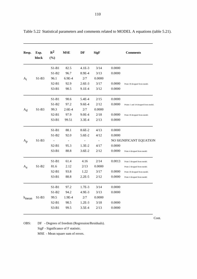
110
Table 5.22 Statistical parameters and comments related to MODEL A equations (table 5.21).
_________________________________________________________________
Resp. Exp. R2 MSE DF SigF Commentsblock (%)
_________________________________________________________________S1-B1 82.5 4.1E-3 3/14 0.0000S1-B2 96.7 8.9E-4 3/13 0.0000
At S1-B3 96.1 6.9E-4 2/7 0.0000S2-B1 92.9 2.6E-3 3/17 0.0000 Point 18 dropped from model.
S3-B1 98.5 9.1E-4 3/12 0.0000_________________________________________________________________
S1-B1 98.6 5.4E-4 2/15 0.0000S1-B2 97.2 9.6E-4 2/12 0.0000 Points 1 and 14 dropped from model.
Ad S1-B3 99.3 2.6E-4 2/7 0.0000S2-B1 97.9 9.0E-4 2/18 0.0000 Point 18 dropped from model.
S3-B1 99.51 3.3E-4 2/13 0.0000_________________________________________________________________
S1-B1 88.1 8.6E-2 4/13 0.0000S1-B2 92.0 5.6E-2 4/12 0.0000
Ap S1-B3 - - - - NO SIGNIFICANT EQUATIONS2-B1 95.3 1.3E-2 4/17 0.0000S3-B1 88.8 3.6E-2 2/12 0.0000 Point 4 dropped from model.
_________________________________________________________________S1-B1 61.4 4.16 2/14 0.0013 Point 3 dropped from model.
Aa S1-B2 81.6 2.12 2/13 0.0000 Point 2 dropped from model.
S2-B1 93.8 1.22 3/17 0.0000 Point 18 dropped from model.
S3-B1 88.8 2.2E-5 2/12 0.0000 Point 4 dropped from model.
_________________________________________________________________S1-B1 97.2 1.7E-3 3/14 0.0000S1-B2 94.2 4.9E-3 3/13 0.0000
hmean S1-B3 99.5 1.9E-4 2/7 0.0000S2-B1 98.5 1.2E-3 3/18 0.0000S3-B1 99.5 3.5E-4 2/13 0.0000
_________________________________________________________________Cont.
OBS: DF - Degrees of freedom (Regression/Residuals).SigF - Significance of F statistic.MSE - Mean square sum of errors.
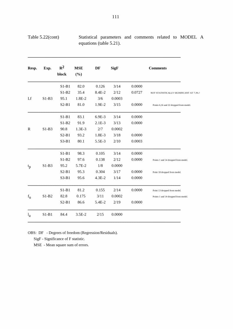
111
Table 5.22(cont) Statistical parameters and comments related to MODEL Aequations (table 5.21).
_________________________________________________________________
Resp. Exp. R2 MSE DF SigF Commentsblock (%)
_________________________________________________________________S1-B1 82.0 0.126 3/14 0.0000S1-B2 35.4 8.4E-2 2/12 0.0727 NOT STATISTICALLY SIGNIFICANT AT 7.3% !
Lf S1-B3 95.1 1.8E-2 3/6 0.0003S2-B1 81.0 1.9E-2 3/15 0.0000 Points 6,16 and 22 dropped from model.
_________________________________________________________________S1-B1 83.1 6.9E-3 3/14 0.0000S1-B2 91.9 2.1E-3 3/13 0.0000
R S1-B3 90.8 1.3E-3 2/7 0.0002S2-B1 93.2 1.8E-3 3/18 0.0000S3-B1 80.1 5.5E-3 2/10 0.0003
_________________________________________________________________S1-B1 98.3 0.105 3/14 0.0000S1-B2 97.6 0.138 2/12 0.0000 Points 1 and 14 dropped from model.
tp S1-B3 95.2 5.7E-2 1/8 0.0000S2-B1 95.3 0.304 3/17 0.0000 Point 18 dropped from model.
S3-B1 95.6 4.3E-2 1/14 0.0000_________________________________________________________________
S1-B1 81.2 0.155 2/14 0.0000 Point 13 dropped from model.
fu S1-B2 82.8 0.175 3/11 0.0002 Points 1 and 14 dropped from model.
S2-B1 86.6 5.4E-2 2/19 0.0000_________________________________________________________________la S1-B1 84.4 3.5E-2 2/15 0.0000_________________________________________________________________
OBS: DF - Degrees of freedom (Regression/Residuals). SigF - Significance of F statistic. MSE - Mean square sum of errors.

112
Table 5.23 MODEL B type equations.
____________________________________________________________________________________
RESP. EXP. MODELLING EQUATIONSSTEP
____________________________________________________________________________________
At S1-B1 ln(y) = 10.584 - 0.955w - 0.413v + 0.0016Iw - 0.0019Ig + 0.0255wv + 0.046wg (1.335) (0.188) (0.123) (0.0003) (0.0005) (0.0100) (0.012)
____________________________________________________________________________________
S1-B1 y = -2.87 + 0.701I - 14.28w - 0.0798Ig + 1.664wgAp (3.39) (0.078) (1.71) (0.0108) (0.238)
------------------------------------------------------------------------S2-B1 ln(y) = -7.413 + 0.0458I - 0.137w + 1.31g - 0.0043Ig - 0.0482vg
(2.745) (0.0100) (0.034) (0.39) (0.0014) (0.0025)____________________________________________________________________________________
S1-B2 y = 52.4 - 0.467I + 0.0194Iw + 0.0460Ig - 0.780wg (22.7) (0.166) (0.0070) (0.0120) (0.269)
Aa ------------------------------------------------------------------------S2-B1 y2 = -2609. + 22.4I - 256.w + 349.w - 2.67Iv + 29.0wv
(1973.) (5.3) (57.) (138.) (0.77) (8.3)____________________________________________________________________________________
R S1-B2 y = 2.049 - 0.277v + 0.0189wv - 0.0092wg (0.080) (0.018) (0.0013) (0.0007)
____________________________________________________________________________________
S1-B1 y = -37.9 + 4.30w + 3.85v - 0.0028Iw - 0.365wv (8.6) (0.74) (1.21) (0.0005) (0.100)-----------------------------------------------------------------------
Lf S1-B3 ln(y + 0.5) = 20.336 - 0.0873I - 2.464v + 0.0017Iw + 0.0080Iv (6.032) (0.0237) (0.841) (0.0002) (0.0033)------------------------------------------------------------------------
S2-B1 ln(0.5 - y) = -1.930 + 0.0165I - 0.126w - 0.00073Ig (0.662) (0.0025) (0.049) (0.00010)
____________________________________________________________________________________
S1-B1 y1/2= -3.43 + 0.0294I - 0.0012Iw + 0.0014Iv - 0.0028Ig - 0.0297wv + 0.0587wg (1.05) (0.0079) (0.0003) (0.0005) (0.0005) (0.0089) (0.0060)
fu ------------------------------------------------------------------------S1-B2 ln(y) = 8.996 + 1.598w - 4.906g - 0.0053Iw + 0.0117Ig - 0.110wv + 0.186vg
(1.080) (0.627) (1.086) (0.0021) (0.0035) (0.038) (0.067)____________________________________________________________________________________
OBS:Numbers in brackets are the standard deviation estimates of the regression coeficients.
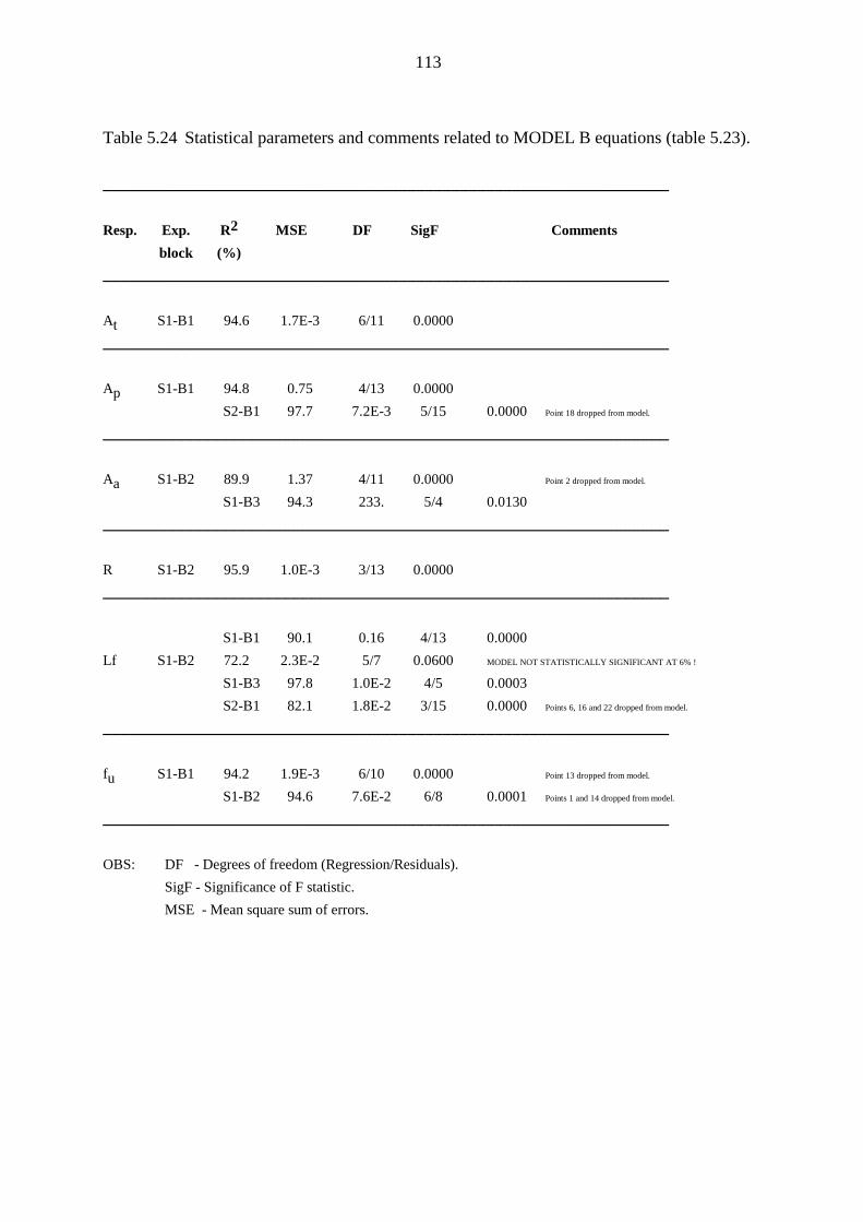
113
Table 5.24 Statistical parameters and comments related to MODEL B equations (table 5.23).
_________________________________________________________________
Resp. Exp. R2 MSE DF SigF Commentsblock (%)
_________________________________________________________________
At S1-B1 94.6 1.7E-3 6/11 0.0000_________________________________________________________________
Ap S1-B1 94.8 0.75 4/13 0.0000S2-B1 97.7 7.2E-3 5/15 0.0000 Point 18 dropped from model.
_________________________________________________________________
Aa S1-B2 89.9 1.37 4/11 0.0000 Point 2 dropped from model.
S1-B3 94.3 233. 5/4 0.0130_________________________________________________________________
R S1-B2 95.9 1.0E-3 3/13 0.0000_________________________________________________________________
S1-B1 90.1 0.16 4/13 0.0000Lf S1-B2 72.2 2.3E-2 5/7 0.0600 MODEL NOT STATISTICALLY SIGNIFICANT AT 6% !
S1-B3 97.8 1.0E-2 4/5 0.0003S2-B1 82.1 1.8E-2 3/15 0.0000 Points 6, 16 and 22 dropped from model.
_________________________________________________________________
fu S1-B1 94.2 1.9E-3 6/10 0.0000 Point 13 dropped from model.
S1-B2 94.6 7.6E-2 6/8 0.0001 Points 1 and 14 dropped from model.
_________________________________________________________________
OBS: DF - Degrees of freedom (Regression/Residuals).SigF - Significance of F statistic.MSE - Mean square sum of errors.
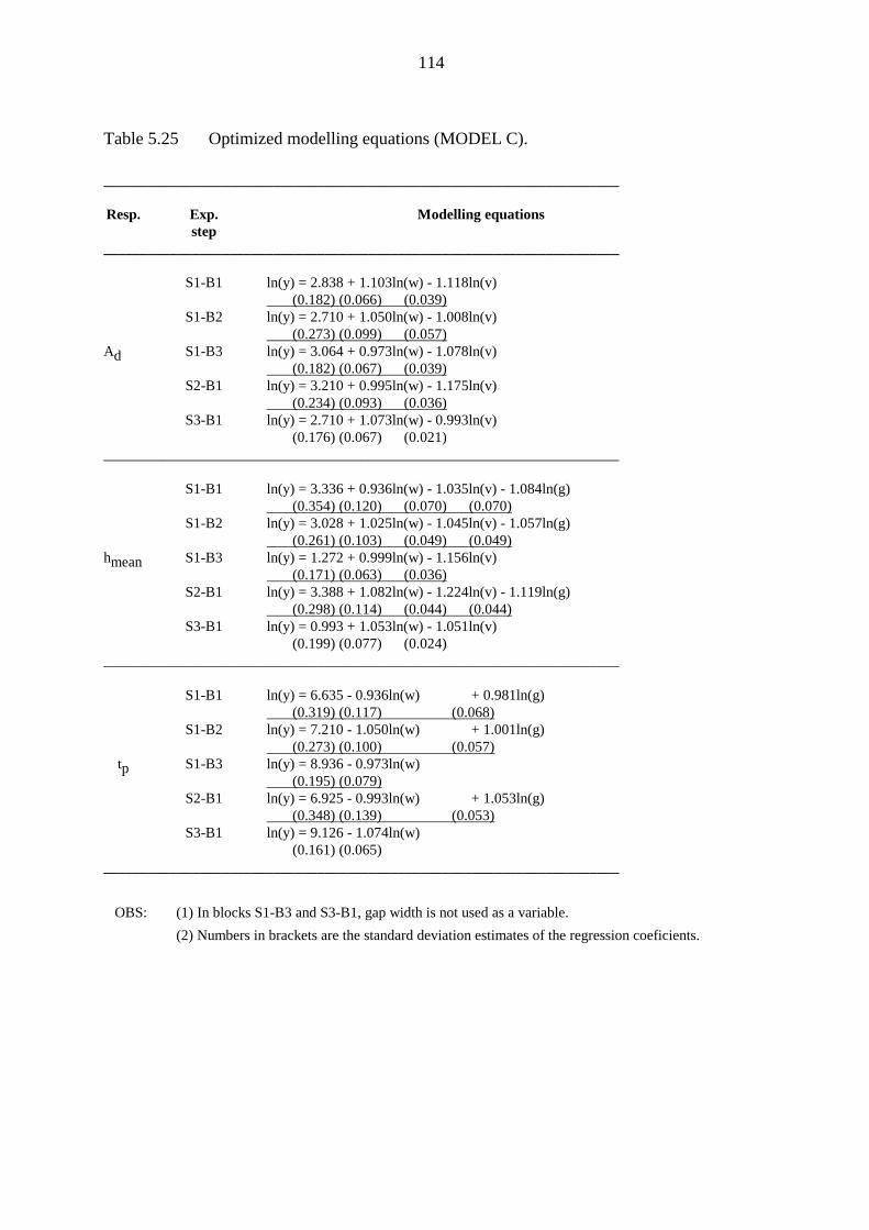
114
Table 5.25 Optimized modelling equations (MODEL C).
______________________________________________________________________
Resp. Exp. Modelling equationsstep
______________________________________________________________________
S1-B1 ln(y) = 2.838 + 1.103ln(w) - 1.118ln(v) (0.182) (0.066) (0.039)
S1-B2 ln(y) = 2.710 + 1.050ln(w) - 1.008ln(v) (0.273) (0.099) (0.057)
Ad S1-B3 ln(y) = 3.064 + 0.973ln(w) - 1.078ln(v) (0.182) (0.067) (0.039)
S2-B1 ln(y) = 3.210 + 0.995ln(w) - 1.175ln(v) (0.234) (0.093) (0.036)
S3-B1 ln(y) = 2.710 + 1.073ln(w) - 0.993ln(v) (0.176) (0.067) (0.021)
______________________________________________________________________
S1-B1 ln(y) = 3.336 + 0.936ln(w) - 1.035ln(v) - 1.084ln(g) (0.354) (0.120) (0.070) (0.070)
S1-B2 ln(y) = 3.028 + 1.025ln(w) - 1.045ln(v) - 1.057ln(g) (0.261) (0.103) (0.049) (0.049)
hmean S1-B3 ln(y) = 1.272 + 0.999ln(w) - 1.156ln(v) (0.171) (0.063) (0.036)
S2-B1 ln(y) = 3.388 + 1.082ln(w) - 1.224ln(v) - 1.119ln(g) (0.298) (0.114) (0.044) (0.044)
S3-B1 ln(y) = 0.993 + 1.053ln(w) - 1.051ln(v) (0.199) (0.077) (0.024)
______________________________________________________________________
S1-B1 ln(y) = 6.635 - 0.936ln(w) + 0.981ln(g) (0.319) (0.117) (0.068)
S1-B2 ln(y) = 7.210 - 1.050ln(w) + 1.001ln(g) (0.273) (0.100) (0.057)
tp S1-B3 ln(y) = 8.936 - 0.973ln(w) (0.195) (0.079)
S2-B1 ln(y) = 6.925 - 0.993ln(w) + 1.053ln(g) (0.348) (0.139) (0.053)
S3-B1 ln(y) = 9.126 - 1.074ln(w) (0.161) (0.065)
______________________________________________________________________
OBS: (1) In blocks S1-B3 and S3-B1, gap width is not used as a variable.(2) Numbers in brackets are the standard deviation estimates of the regression coeficients.
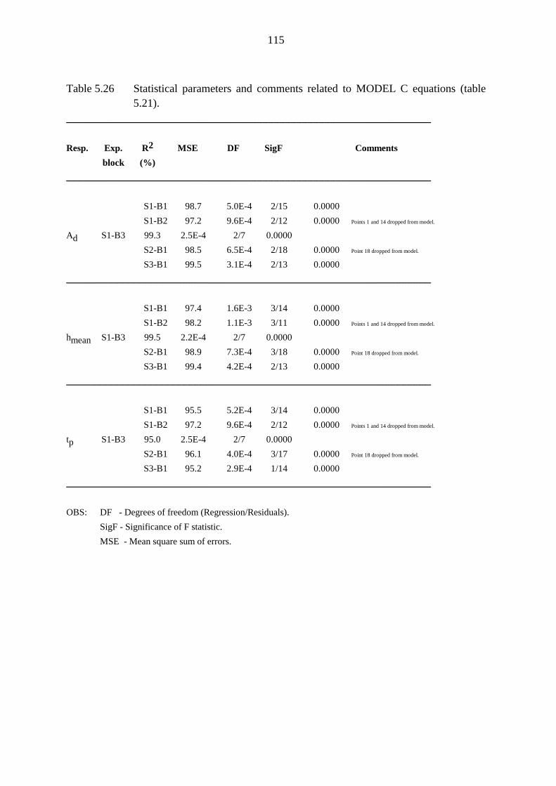
115
Table 5.26 Statistical parameters and comments related to MODEL C equations (table5.21).
_________________________________________________________________
Resp. Exp. R2 MSE DF SigF Commentsblock (%)
_________________________________________________________________
S1-B1 98.7 5.0E-4 2/15 0.0000S1-B2 97.2 9.6E-4 2/12 0.0000 Points 1 and 14 dropped from model.
Ad S1-B3 99.3 2.5E-4 2/7 0.0000S2-B1 98.5 6.5E-4 2/18 0.0000 Point 18 dropped from model.
S3-B1 99.5 3.1E-4 2/13 0.0000_________________________________________________________________
S1-B1 97.4 1.6E-3 3/14 0.0000S1-B2 98.2 1.1E-3 3/11 0.0000 Points 1 and 14 dropped from model.
hmean S1-B3 99.5 2.2E-4 2/7 0.0000S2-B1 98.9 7.3E-4 3/18 0.0000 Point 18 dropped from model.
S3-B1 99.4 4.2E-4 2/13 0.0000_________________________________________________________________
S1-B1 95.5 5.2E-4 3/14 0.0000S1-B2 97.2 9.6E-4 2/12 0.0000 Points 1 and 14 dropped from model.
tp S1-B3 95.0 2.5E-4 2/7 0.0000S2-B1 96.1 4.0E-4 3/17 0.0000 Point 18 dropped from model.
S3-B1 95.2 2.9E-4 1/14 0.0000_________________________________________________________________
OBS: DF - Degrees of freedom (Regression/Residuals).SigF - Significance of F statistic.MSE - Mean square sum of errors.
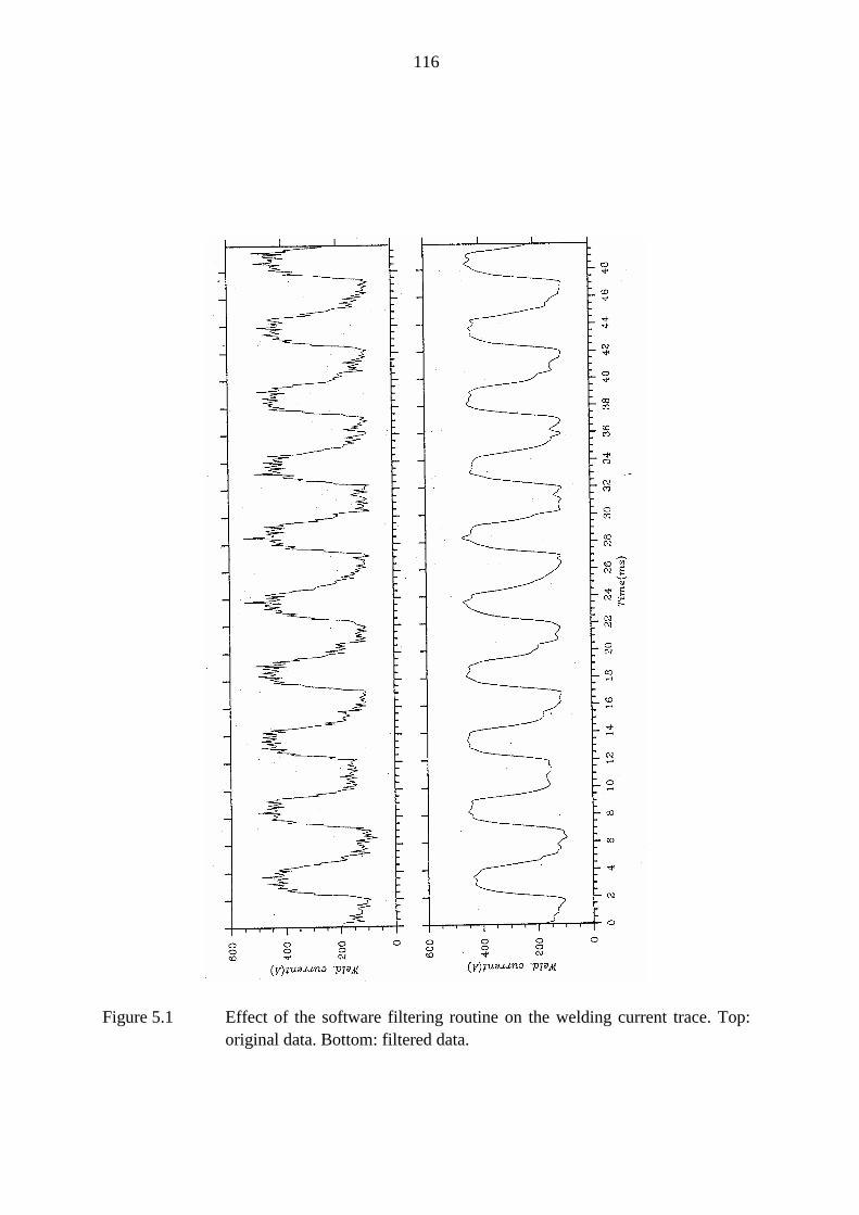
116
Figure 5.1 Effect of the software filtering routine on the welding current trace. Top:original data. Bottom: filtered data.
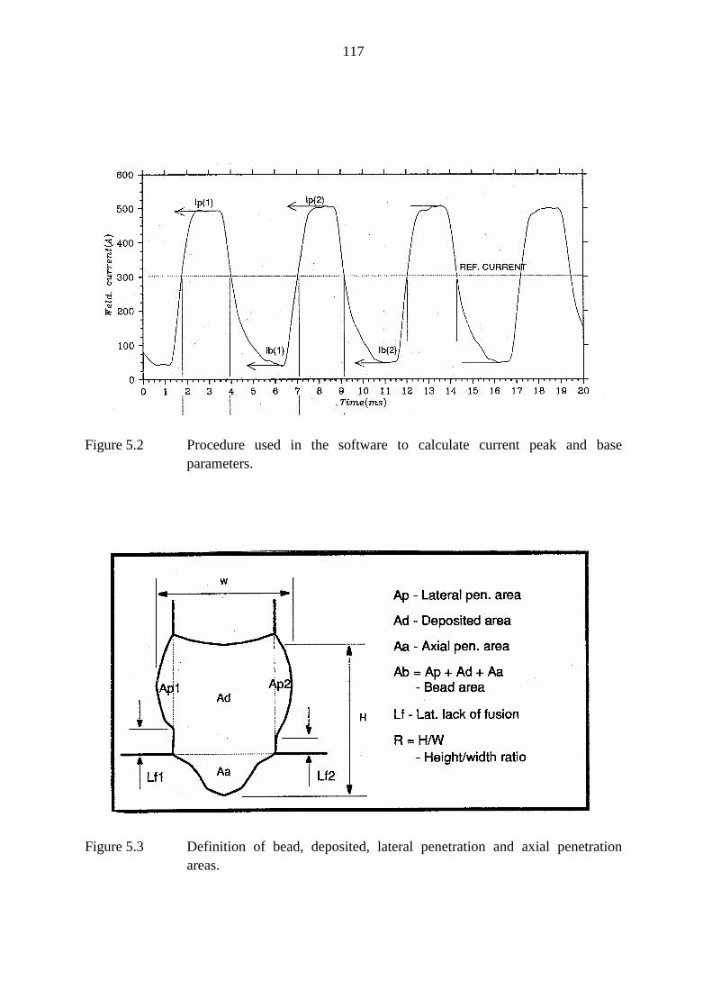
117
Figure 5.2 Procedure used in the software to calculate current peak and baseparameters.
Figure 5.3 Definition of bead, deposited, lateral penetration and axial penetrationareas.
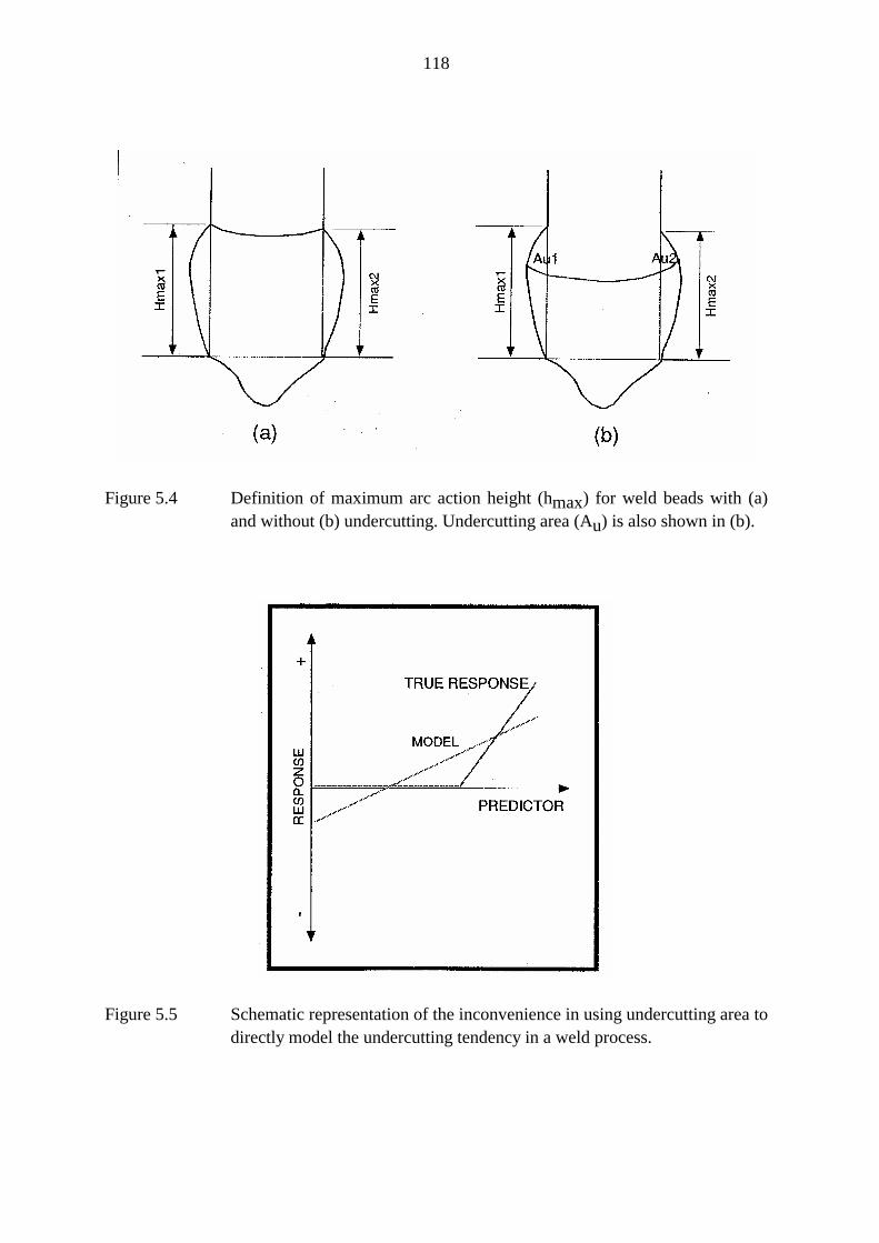
118
Figure 5.4 Definition of maximum arc action height (hmax) for weld beads with (a)and without (b) undercutting. Undercutting area (Au) is also shown in (b).
Figure 5.5 Schematic representation of the inconvenience in using undercutting area todirectly model the undercutting tendency in a weld process.
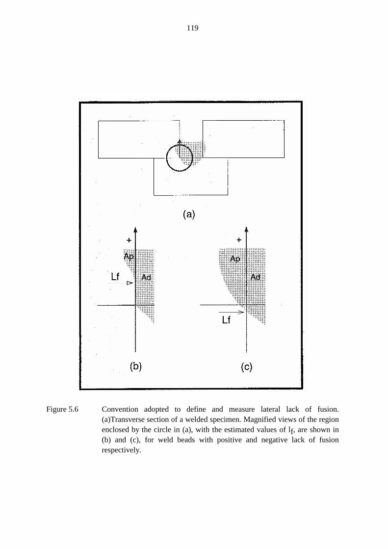
119
Figure 5.6 Convention adopted to define and measure lateral lack of fusion.(a)Transverse section of a welded specimen. Magnified views of the regionenclosed by the circle in (a), with the estimated values of lf, are shown in(b) and (c), for weld beads with positive and negative lack of fusionrespectively.
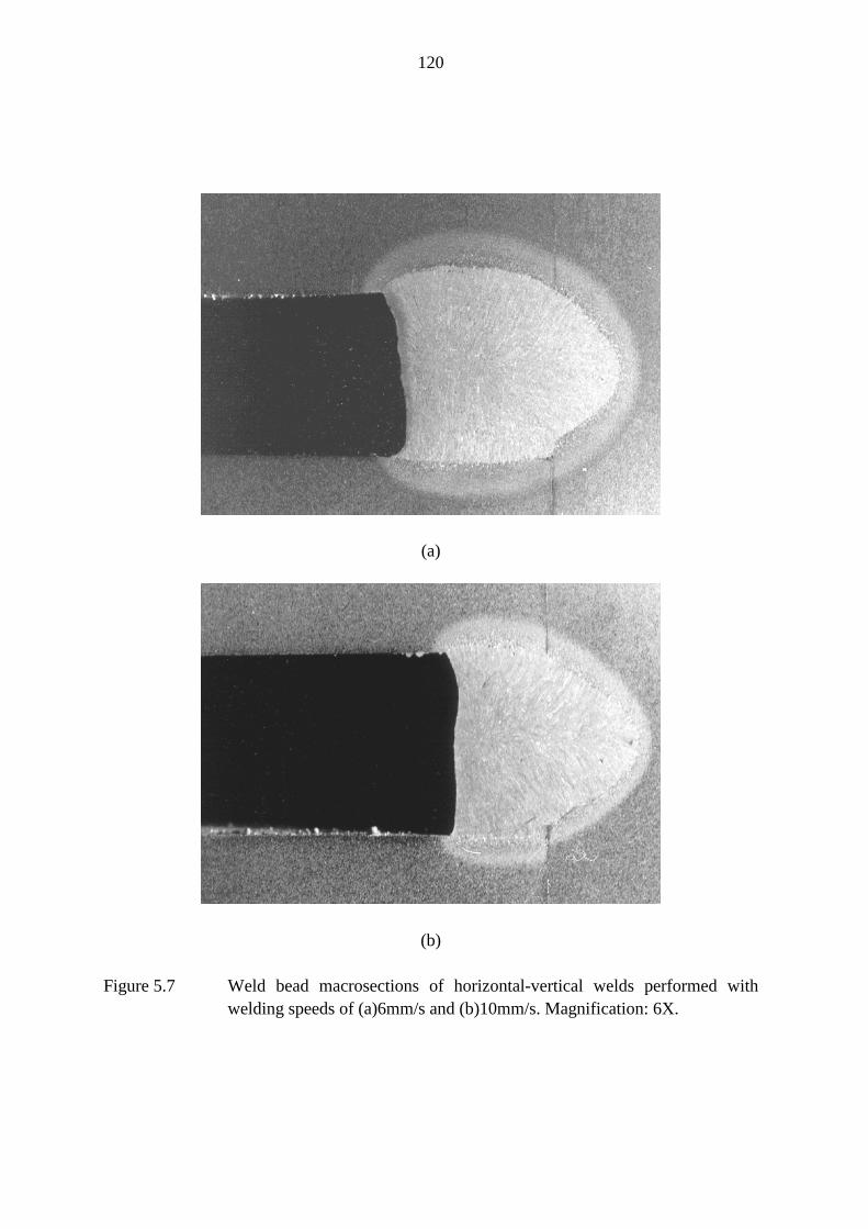
120
(a)
(b)
Figure 5.7 Weld bead macrosections of horizontal-vertical welds performed withwelding speeds of (a)6mm/s and (b)10mm/s. Magnification: 6X.
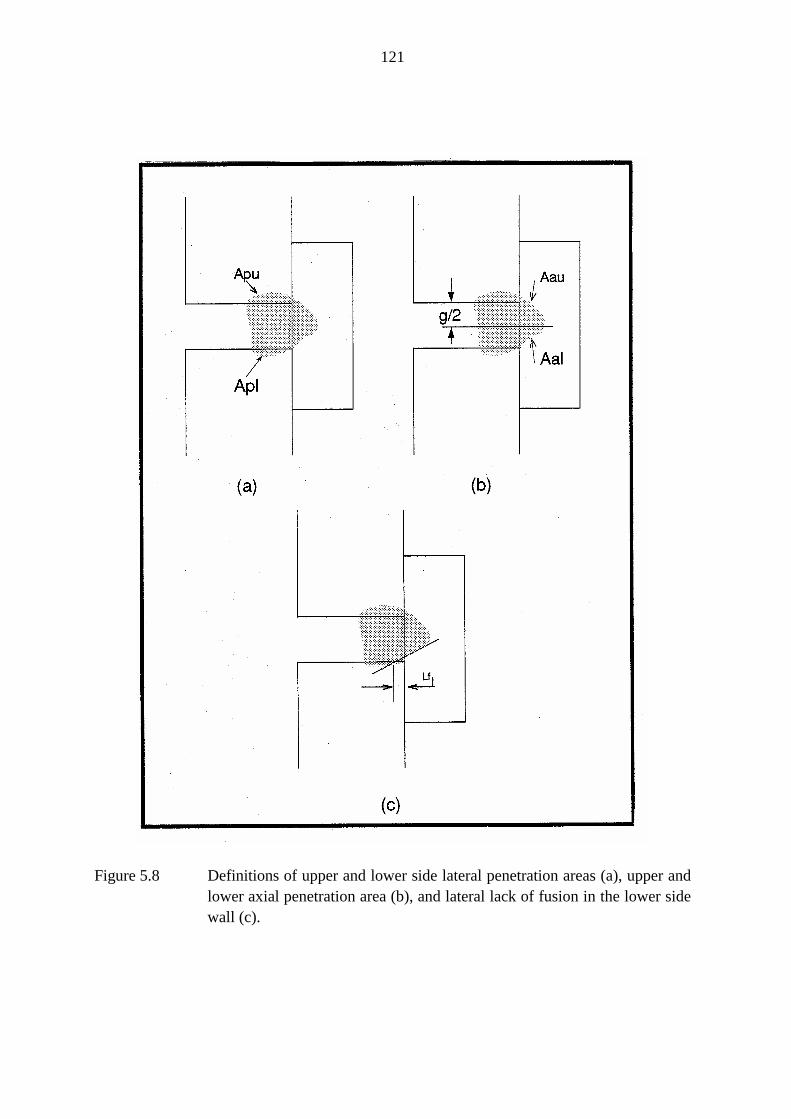
121
Figure 5.8 Definitions of upper and lower side lateral penetration areas (a), upper andlower axial penetration area (b), and lateral lack of fusion in the lower sidewall (c).
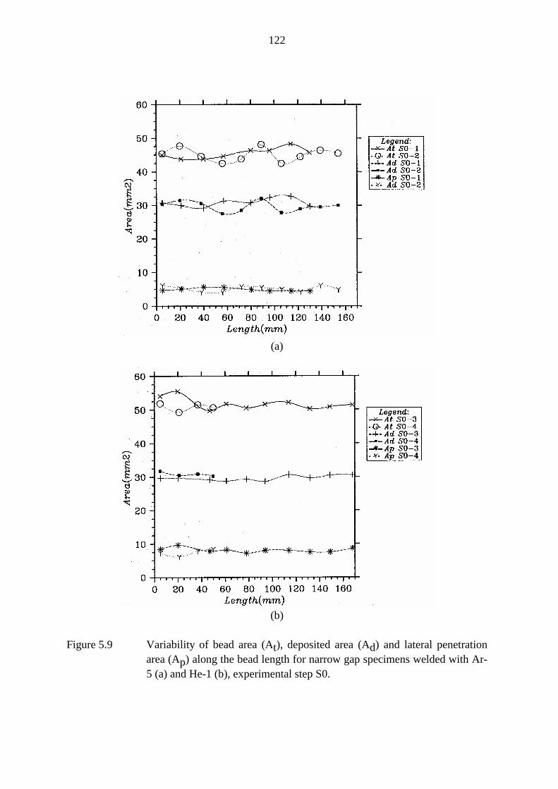
122
(a)
(b)
Figure 5.9 Variability of bead area (At), deposited area (Ad) and lateral penetrationarea (Ap) along the bead length for narrow gap specimens welded with Ar-5 (a) and He-1 (b), experimental step S0.
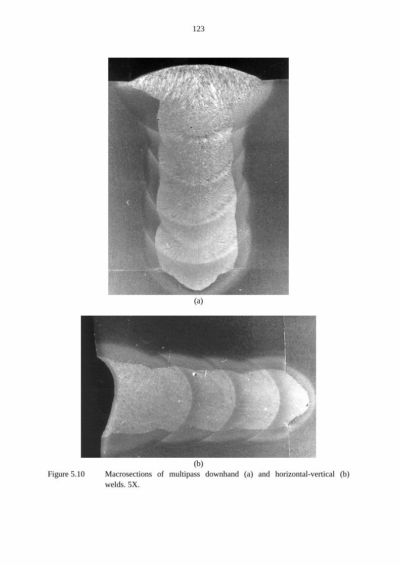
123
(a)
(b)Figure 5.10 Macrosections of multipass downhand (a) and horizontal-vertical (b)
welds. 5X.
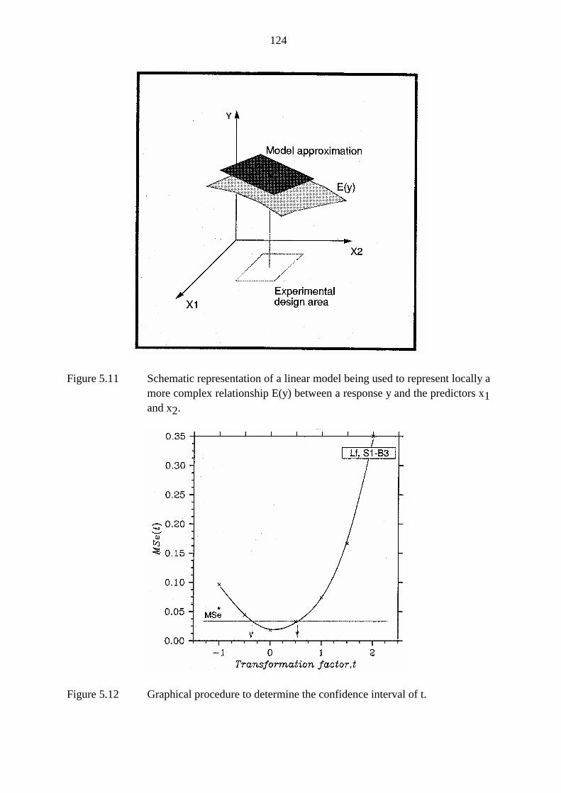
124
Figure 5.11 Schematic representation of a linear model being used to represent locally amore complex relationship E(y) between a response y and the predictors x1and x2.
Figure 5.12 Graphical procedure to determine the confidence interval of t.
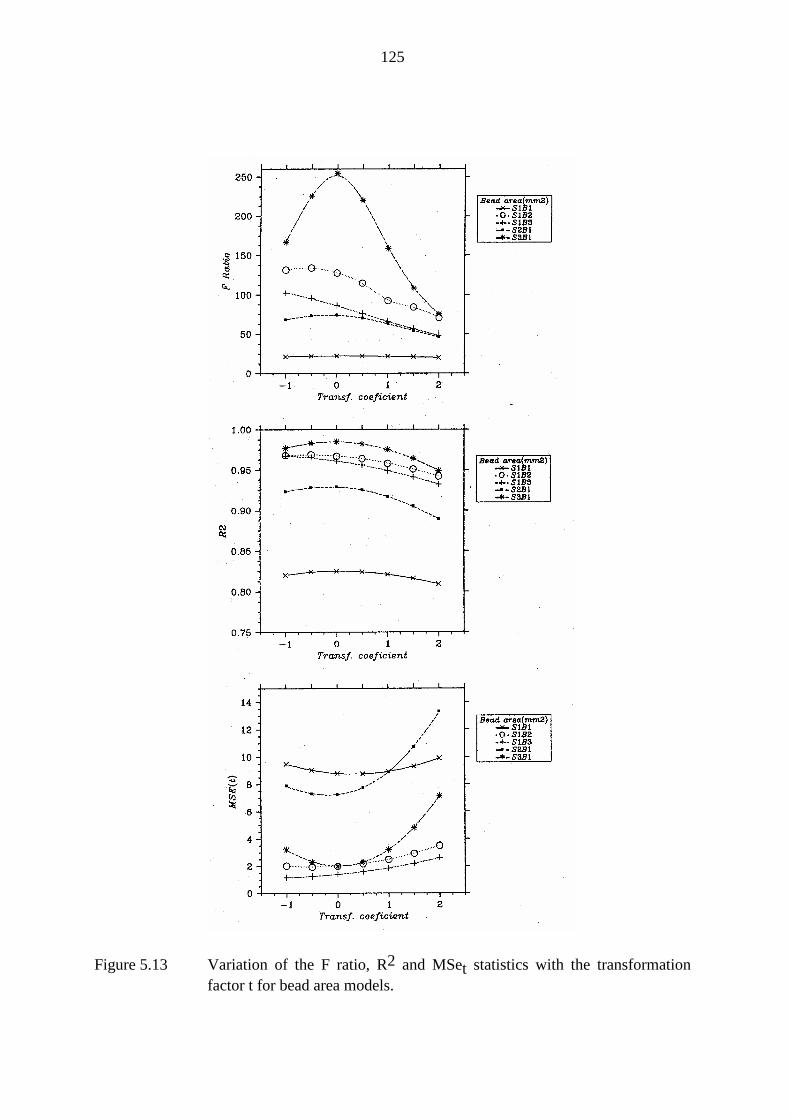
125
Figure 5.13 Variation of the F ratio, R2 and MSet statistics with the transformationfactor t for bead area models.
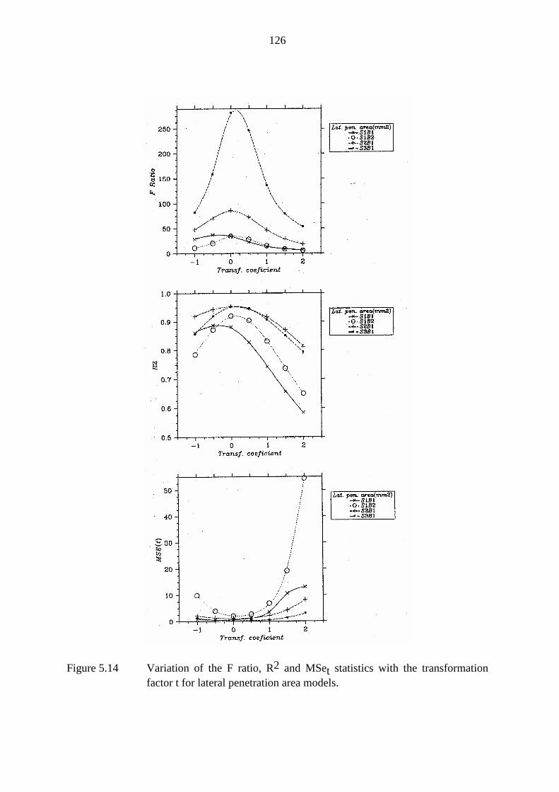
126
Figure 5.14 Variation of the F ratio, R2 and MSet statistics with the transformationfactor t for lateral penetration area models.
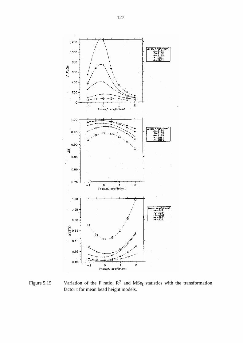
127
Figure 5.15 Variation of the F ratio, R2 and MSet statistics with the transformationfactor t for mean bead height models.
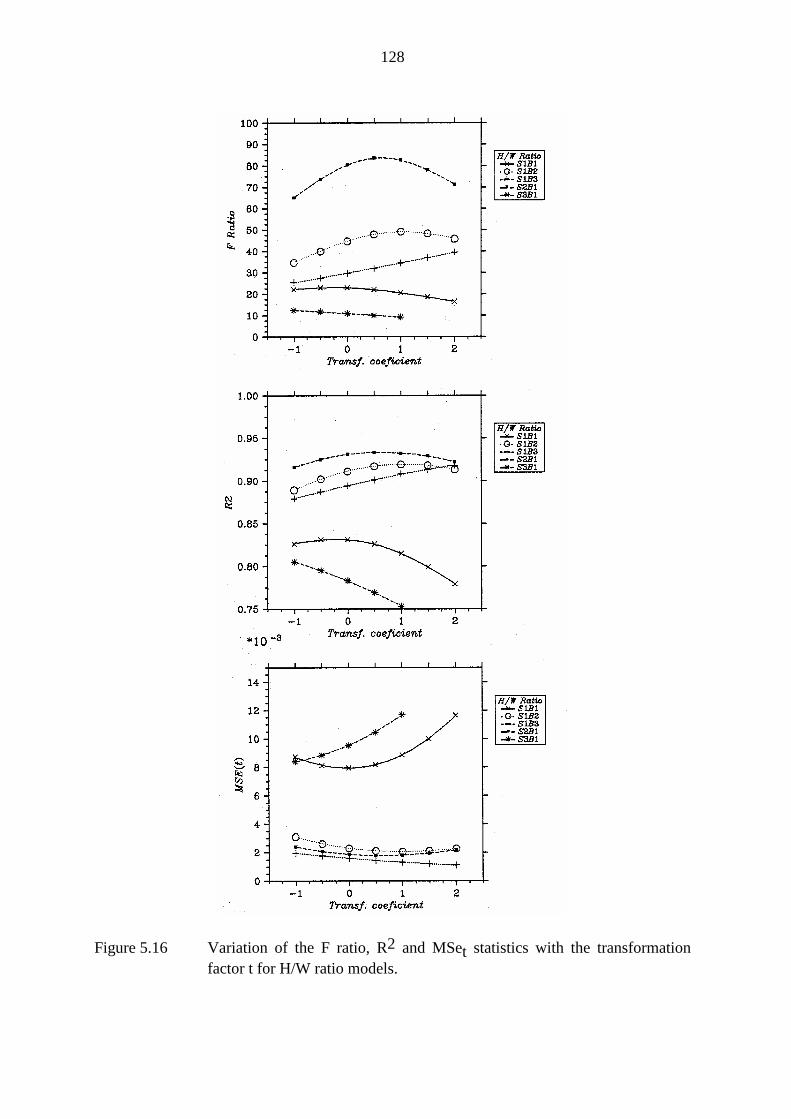
128
Figure 5.16 Variation of the F ratio, R2 and MSet statistics with the transformationfactor t for H/W ratio models.
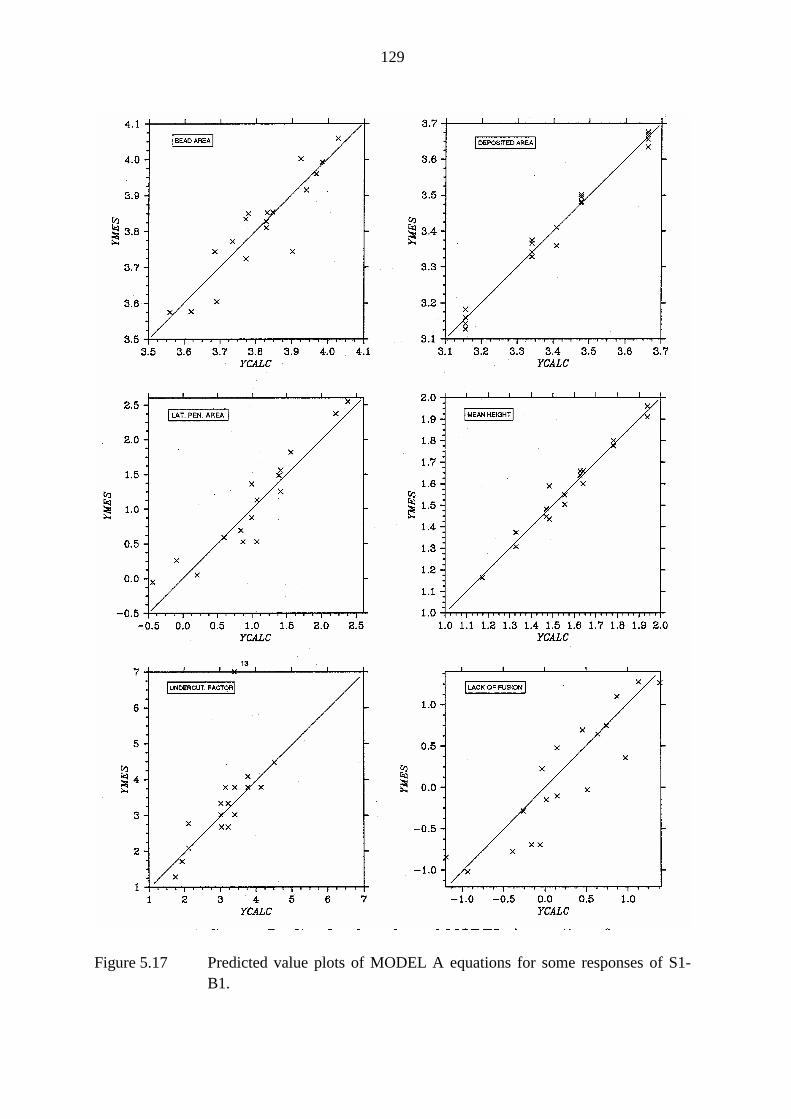
129
Figure 5.17 Predicted value plots of MODEL A equations for some responses of S1-B1.
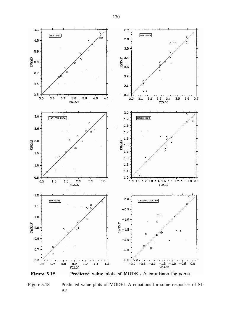
130
Figure 5.18 Predicted value plots of MODEL A equations for some responses of S1-B2.
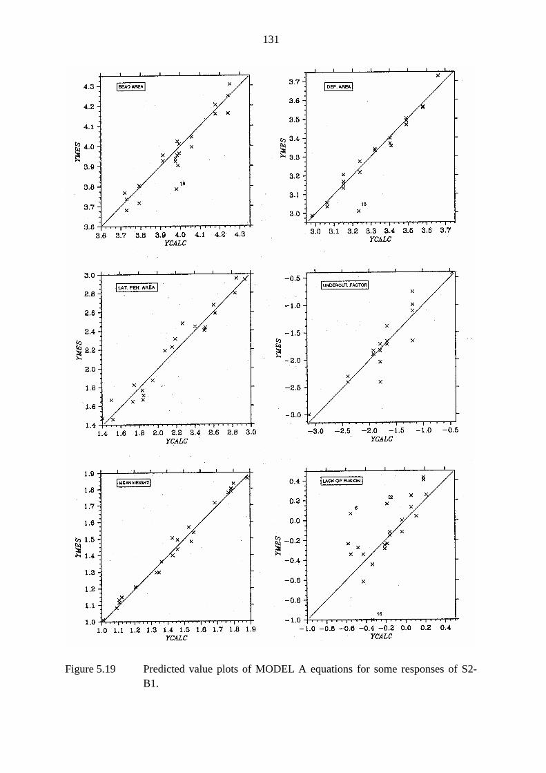
131
Figure 5.19 Predicted value plots of MODEL A equations for some responses of S2-B1.

CHAPTER 6
133
6. Analysis of results and discussion
6.1.Assessment of experimental and modelling techniques
6.1.1.Experimental design
In general, the expected value of a response considered of interest for welding or any otherprocess can be often described by some sort of function F that depends on a number of inputvariables or parameters:
y = F( x1, x2, . . . , xt) [6.1]
Where xi, i=1, t, is a subset of an ideal collection of "all possible parameters of the process".Unfortunately, both F and the subset xi are often partially or completely unknown and theirdetermination may not be simple, or even possible, in some cases. In order to find F, basicphysical principles should be applied to the situation encountered in the welding system anda solution found. However, developing such a model in a comprehensive way for a complexwelding process can be a rather difficult task. Compromise solutions can be frequentlyworked out by making simplifications of the initial assumptions. Although such approach hasgreatly helped the understanding of physical phenomena in welding processes and despiteenormous recent progress in this area, direct application of theoretical principles to a weldingsystem is still mainly limited to general aspects of the process and has found only partialsuccess in modelling a concrete welding application.
Empirical model building has been used as an alternative to the theoretical approach to studywelding processes, particularly if it is desired to approximate the response only over limitedranges of the input variables. By assuming that the corrected form of F is unknown, thisapproach attempts to developed a model of the form:
y = G( x1, x2, . . . , xp) [6.2]
Where G is an arbitrary function that is generally much simpler than F and xi, i=1, p, is a setof input variables not necessarily identical to the one associated with F. Often, the modelabove is based almost completely on information contained in data from actual weldingtrials. Consequently, an empirical model actually represents the data it is derived from, andadopting it to represent a system implies assuming that the available data represent thatsystem well.

134
Therefore, a close link should exist between data collection and model formulation. In thissense, statistical techniques provide a powerful tool for both model building and design ofthe experiment. The former use of statistics has been applied to welding problems for a longtime while the latter has only recently been more commonly applied. A properly designedexperiment can greatly help to reduce confusing effects from experimental error, detect thepresence of complex effects of input variables on the response and provide a more soundbasis for deducing cause-and-effect relationships from the experimental data. Factorialdesign is a statistical experimental technique that is extensively used in industrialexperimentation and has recently proven suitable to the study of welding problems(§2.4.3.2).
In the present programme, the experimental work was initially intended to be designed asfactorial experiments. However, due to the complex interaction that can exist between inputvariables, including joint geometry and power supply characteristics, this approach soonpresented difficulties in terms of guaranteeing stable welding conditions for all experimentaltrials within a factorial block. This represented a limitation of the technique because thewhole experiment is run as a block and the presence of one or more abnormal points canstrongly affect and distort the data analysis step. Therefore, a proper selection of inputvariable levels that provide representative welding conditions is extremely important but afrequently difficult or even impossible task. The knowledge necessary for this selection is notalways completely available at the moment of design and, in many situations, this is one ofthe goals of the experiment. Running an initial set of experimental trials can provide valuableguidance to establish the experimental area, however, this will inevitably add more steps tothe experimental programme and increase its cost.
Furthermore, stable welding conditions will often be naturally linked with a stronginterdependence between some of the input variables and that will complicate the applicationof factorials. For instance, if current and voltage are both to be set at "low" and "high" levelsin a factorial experiment, it may possibly happen that operational conditions will be adequatefor (Vlow,Ilow) and (Vhigh,Ihigh) trials but difficulties can be expected in running both(Vlow,Ihigh) and (Vhigh,Ilow) trials if the difference both in I and V between the "high" and"low" levels is sufficiently high. Reducing the difference between levels could increase thepossibility of generating stable operational conditions for most of the trials. Unfortunatelythis would also increase the relative participation of the experimental error in the data.Another alternative would be to run the factorial with some of the input variablestransformed into more suitable formats, for instance the use of the ratio (V/I) instead of I andV separated. This may, however, complicate interpretation of the final model.
135
In the present programme, a truly factorial scheme was substituted, in experimental steps S2and S3, by an experimental design where not all of the input variables were perfectlyorthogonal with some of the others in order to adjust the experiment to the naturalrequirements of the process. While this approach may complicate later data analysis byintroducing some collinearity into the model, distortion of the initial factorial experiment waslimited to those variables in which previous results had indicated the necessity of thisadjustment.
6.1.2.Data analysis
The selection of the initial set of candidate input variables to be included in model buildingmay have a profound influence in the final form of the model. For instance, in experimentalstep S1, a first modelling exercise was performed using pulse frequency (F), wire feed rate(w), welding speed (v) and gap width (g) as initial variable candidates. The resulting modelfor arc length in S1-B1 after variables selection was:
ln(la) = 2.210 + 0.015F - 0.29w - 0.11g [6.3a]
which detected a significant effect of gap width on arc length. Later work using slightlydifferent initial variable candidates (mean current, wire feed rate, welding speed and gapwidth) did not detect any influence of gap width. At least two hypotheses may be presentedin order to explain this apparent discrepancy. Firstly, the weld pool level can be considered tobe raised by the constraining effect of the joint side walls resulting in an apparent decrease instandoff distance. This effect would be inversely proportional to the gap width and, inassociation with the constant voltage operation of the power supply during peak period,would cause an increase in current and arc length. Alternatively and more probably, theinteraction between joint geometry and power supply characteristic (see §6.4) could explainan increase in both current level and arc length for the narrower gap operation. In both cases,the influence of gap in arc length would be associated with variations in welding current.
Therefore, when current was included as an initial variable candidate and selected as asignificant factor to describe arc length variation, it incorporated in the model most of theinformation that was associated in the previous equation with gap width which was then notconsidered significant by the variable selection routine. Compared with the initial equation,the latter one,
ln(la) = 1.065 + 0.0199I - 0.456w [6.3b]
136
does not apparently reflect the interaction between power supply characteristic and jointgeometry. The initial input variable set containing welding current and wire feed rate wasadopted and used in the present work for all response variables, even though this selection isnot the most commonly employed in welding research where current and voltage are moreoften preferred. Among the reasons for this choice, it can be mentioned the determination ofsimpler models for some responses and the fact that current and wire feed rate were thevariables directly controlled in the two last experimental blocks.
The selection of an initial set of predictor variables depends on many factors, some of themof a subjective nature such as motivation and the experience of the researcher. Manydifferent alternatives may be possible and equally suitable. One important consideration is toavoid whenever possible the situation in which collinearity problems are incorporated in thepredictors set with the result that they would greatly affect data analysis and result in a modelthat, although fitting the experimental data well, may have very little connection with the realsystem. The close link between final model form, initial predictors set and experimentaldesign is a basic characteristic of statistical modelling. The consequence is that results ofempirical models tend to be very specific and extrapolation to other systems should be donevery cautiously.
In the present programme, data analysis was made up of four inter-related steps: selection ofdependent variable transformation, selection of the "best" subset of input variables, modelfitting and model diagnosis (§5.3). Transformation was found to be an important measure toimprove modelling results with few of the final equations (Model A) being developed on theoriginal, untransformed responses (i. e., with a transformation factor of one). The resultantmodelling equations with transformed response tended to be simpler and easier to interpretthan alternative models with included interaction between input variables (model B). Ingeneral, the first three modelling steps can be fairly well automated by means of modernstatistical software packages. However, the forth step is, in its simpler and more usual formas employed here, strongly dependent on the visual interpretation of plots and, therefore, apackage that provides good interactive facilities at some stages of the process can result in amore efficient tool than a fully automated one.
6.2.Bead characteristics
A large number of parameters were defined and used to characterize weld bead geometry anddefect formation in the present work. A direct analysis of all these parameters across fivedifferent experimental blocks would result in a very lengthy and confusing process.Therefore, in an attempt to simplify the analysis of results, a three-step approach was
137
followed. In a first step (present section), general weld bead characteristics were grouped intothree classes before being analysed by studying the main features of their modellingequations. A graphical approach to represent process operation characteristics was developedand analysed in section §6.3. Finally, aspects relevant to horizontal-vertical welding will bediscussed in section §6.4.
The weld bead is formed by material provided from two sources: (a)filler metal (wire) and(b) melted portions of the workpiece. Now, most of the parameters introduced in the presentwork can related to one of these sources of material and, based on that, a classification can beworked out to systematize their analysis:
. Bead parameters related with wire fusion: Deposited area (Ad), mean bead height(hmean), and production time (tp).
. Bead parameters related with plate fusion: Lateral penetration area (Ap), axialpenetration area (Aa), and lateral lack of fusion (lf).
. Bead parameters related with both sources: Bead area (At), H/W ratio (R) andundercutting factor (fu).
6.2.1.Bead parameters related with wire fusion
All parameters included in this group can be alternatively represented by simple theoreticalexpressions based on mass balance between melting rate and deposited area (equation[5.12]). This predicted simple behaviour is reflected in the statistical models by a very goodfit of the experimental data and by the absence of a current term in the equations (table 5.21and 5.25) for a initial set of input variables that includes w, v and g. In particular, model Ctype equations for Ad and hmean approximate well to their theoretical counterparts. Forinstance, the mean value of the coefficients for w and v empirically obtained for depositedarea expressions in the five experimental steps are respectively 1.039 and 1.074, very close tothe expected value of one. Therefore, the assumptions of the mass balance model and theexperimental conditions appear to be both satisfactory as far as this class of bead parameter isconcerned.
By comparing the constant term of the theoretical expression for Ad (equation [5.13]) withits empirical values, the expected wire diameter (dwe) for each experimental step can becalculated by:
138
dwe = [(4/k'π)exp(a0)]1/2 [6.4]
where k' is a constant related with the measuring units and equal to 16.7(m.s)(mm.min)-1.Values for dwe calculated by this method are presented in table 6.1. The mean of theestimated values for all experimental steps agrees rather well with the measured wirediameter (1.18mm). However, individual results reveal a large scatter and, if they are used tocalculate metal losses (δm) of the process by:
δm = 100[1 - (dwe/dw)2], [6.5]
metal additions (i. e., δm<0) of over 20% are predicted. Such discrepancies are, however,explained by an inadequate use of the empirical model. Equation [6.4] was obtaining bysetting ln(w) and ln(v) to zero in the empirical model which corresponds to a very largeextrapolation from the conditions used in the experimental blocks. A more adequateexpression would be:
dwe = [(4/k'π)Adc.vc/wc]1/2 [6.6]
where vc and wc are values of v and w corresponding to the central point of the experimentaldesign, which is the point where a minimum in the variability of the predicted values of Ad isespected, and Adc is the calculated deposited area at this location. Calculated values of dweare shown in table 6.2. The individual results match rather well with the measured wirediameter and suggest metal losses under 10% for all experimental steps.
As expected from the mass balance equation, modelling expressions for production timedepend significantly only on wire feed rate and gap width. Figure 6.1 presents surface plotsof production time for experimental blocks S1-B1, S1-B2 and S2-B1. The results from thedifferent blocks are rather similar, the small differences being probably associated with metalloss levels (table 6.2). The results also agree well with those estimated by Fennel (1986) whoexpected a time of 145s to weld a 325mm diameter pipe with a 20mm thick wall using a fourhead GMAW system and a 6-8mm gap.
The simple format, good precision and uniformity amongst experimental blocks of themodelling equations of this section are closely related to the set of initial input variablesadopted and the simple underlying physical model that could be associated with Ad, hmeanand tp. Should a different set of initial input variables be selected so that more complexprocesses would have to be reflected in any model linking input and response, the finalmodels would probably be less uniform and precise.
139
6.2.2.Bead parameters related to plate fusion
6.2.2.1.Introduction
In opposition to the group of parameters discussed above, parameters that are related withplate fusion will more probably depend on how energy from the arc is transferred to theworkpiece and cannot be represented by a simple mass balance model. As this can beexpected to depend on complex interactions of different factors, many of them not wellunderstood, the resulting statistical models are likely to be more complicated and less precisethan the previous ones. Dissimilarities between statistical modelling equations for a givenresponse may provide an indication of differences in process characteristics.
Different mechanisms, such as heat conduction in the workpiece (Christensen et al. 1965,and Quintino 1986), fluid flow in the weld pool (Szekely 1986), impingement of liquid dropsof filler metal on the workpiece (Essers and Walter 1979) and arc pressure (Halmoy 1979)have been associated with and may play a role in plate fusion and penetration. In bead-on-plate GMA welding, plate fusion is characterized by two distinct overlapping regions: (a) amore or less central finger region, which is generally associated with one or both of the twolatter mechanisms, and (b) a shallower and approximately elliptic bath formed possibly byheat conduction in a liquid layer. Finger penetration generally dominates in argon shieldedGMAW, but the relative importance of the two regions varies with current, voltage, travelspeed, gas composition, etc (Gurev and Stout 1963).
In NGW, fusion of the workpiece is more complex because, unlike bead-on-plate or evengroove welding, it is necessary to provide penetration not in one only direction (under theweld pool), but in three different ones, including both sidewalls (Malin 1987). Sidewallfusion is more probably associated with radial heat diffusion from the arc column and may beaffected by arc length and voltage as confirmed by some authors (Kurakawa et al. 1966,Belchuk and Titov 1970, and Matsunawa and Nishiguchi 1979).
In bead-on-plate welding, it is well established that, at low travel speeds, the liquid volume inthe pool can be so high that it tends to flow under the arc cushioning the base metal andimpairing its fusion. A critical travel speed has be found by Quintino for pulsed GMAW ataround 1-3mm/s below which plate penetration is greatly reduced. A similar critical speedcan be expected for NGW conditions which should be displaced to higher travel speeds dueto the confining effect of the side wall on the weld pool (Matsunawa and Nishiguchi 1979).
140
6.2.2.2.Modelling results
Modelling equations for lateral penetration area (Ap) presented the same general form,including the same response transformation, in all experimental blocks that yielded asignificant model. However, important differences in terms of the final set of significantinput variables were found for experimental block S3-B1 which were performed in thehorizontal-vertical position. In the downhand position, Ap increased with current whiledecreasing with wire feed rate, welding speed and gap width as shown by the coefficients ofits modelling equations (table 5.21) and by its surface plots (figure 6.2). The direction ofmaximum increase for a response adequately represented by a model A type equation, in theplane defined by welding current and wire feed rate (I,w), is parallel to the vector mI,w:
[6.7]mI,w = ( 1, αI,w) [6.7]
where αI,w = aw/aI (in Am-1min) is the ratio between the regression coefficients for w and Iin the modelling equations. Calculated values of αI,w for Ap, voltage and arc length areshown in table 6.3. These values are relatively close indicating that a good correlationbetween Ap, V and la may be expected and this is further supported by the similarity ofsurface plots for Ap (figure 6.2), V and la (figure 6.3). Therefore, both V and la can beexpected to significantly influence lateral penetration as would be expected if lateral fusion isdetermined mainly by radial heat transfer for the arc.
In a manner similar to results from other authors (for instance, Foote 1986 and Jackson andSargent 1966), lateral penetration tended to be greater for those experimental blocks thatused a helium based shielding gas. No significant improvement in lateral fusion could beassociated with higher CO2 contents for argon based shielding mixture by comparingexperimental blocks S1-B1 and S1-B3. Results also suggest that, in argon based shielding,regression coefficients in the equation for Ap for both current and wire feed rate aresignificantly greater (in module) than those for helium based shielding. As a result, lateralfusion of the joint can be expected to be more sensitive to changes in current and wire feedrate in argon based shielding.
Although modelling results for lateral lack of fusion (lf) were generally poorer in terms ofstandard of fit than those for Ap, both parameters tended to be influenced by current and wire
141
feed rate in a comparable way but in an opposite direction (figure 6.4). Therefore similarcorrelations between lf, and V or la may also be expected.
For downhand position operation, welding current and gap width are the main input variablescontrolling axial penetration area, Aa (figure 6.5). Aa increases with g possibly by areduction in the confining effect of the side walls on the molten weld pool. In similaroperational conditions, argon based shielding gases tended to present greater Aa, and thismay be associated with a more intense finger action with this shielding gas composition.
An analysis of the general aspects of plate fusion indicates that, among the shielding gascompositions tested in the narrow gap experimental blocks, those employing high heliumcontent show improved lateral fusion of the workpiece as indicated in terms of both Ap andlf. Results also suggest that improved plate fusion characteristics can be associated withsteady direct current operation. In pulsed current operation (particularly with high peakcurrents), wire melting rate tended to be higher than in steady current operation due to thehigher joule heating of the wire (§2.2.4). This difference can be partially explained in termsof the effect of w on the volume of the molten pool. However, even if this effect isdiscounted by overlapping the areas of similar operational conditions in the surface plots offigures 6.2, 6.4 and 6.5, welds using steady current (block S2-B1) will still generate higherplate fusion in both lateral and axial directions than a similar block that operated with pulsedcurrent (S1-B2). This is a different behaviour from that commonly reported in the literaturefor bead-on-plate welding (Foote 1986, Quintino 1986, and Maruo and Hirata 1982) whichindicates only minor differences in plate fusion between pulsed and steady current. Besidescurrent operational mode, another difference between blocks S1-B2 and S2-B1 is related tominor differences in shielding gas composition which may have an important influence inprocess stability (Chapter 7). However, the influence of this effect on plate fusion was notassessed in the present programme.
6.2.3.Bead parameters related to both wire and plate fusion.
Bead area (At) directly results from the sum of Ad, Aa and Ap. Therefore, it can be assumedthat modelling equations for At should reflect the relative influence of the input variables ineach of the parameters above. Based on this assumption, one can expect positive regressioncoefficients for welding current due to its influence on plate fusion (both lateral and axial),and negative ones for welding speed due to its strong influence on deposited area and inlateral penetration. Based on the same assumption, other input variables should be expectedto present less clear influences on the weld bead area. Surface plots for At are shown in
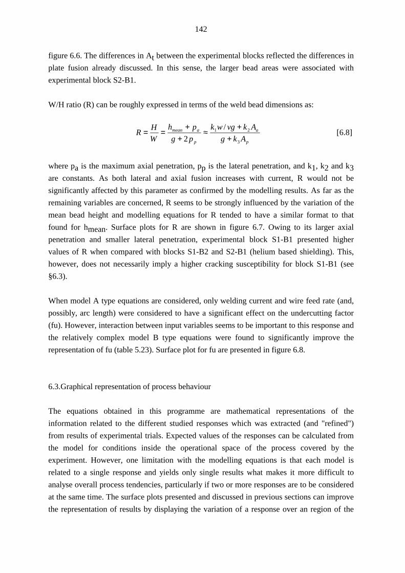
142
figure 6.6. The differences in At between the experimental blocks reflected the differences inplate fusion already discussed. In this sense, the larger bead areas were associated withexperimental block S2-B1.
W/H ratio (R) can be roughly expressed in terms of the weld bead dimensions as:
p
a
p
amean
AkgAkvgwk
pgph
WHR
3
21 /2 +
+≈
++
== [6.8]
where pa is the maximum axial penetration, pp is the lateral penetration, and k1, k2 and k3are constants. As both lateral and axial fusion increases with current, R would not besignificantly affected by this parameter as confirmed by the modelling results. As far as theremaining variables are concerned, R seems to be strongly influenced by the variation of themean bead height and modelling equations for R tended to have a similar format to thatfound for hmean. Surface plots for R are shown in figure 6.7. Owing to its larger axialpenetration and smaller lateral penetration, experimental block S1-B1 presented highervalues of R when compared with blocks S1-B2 and S2-B1 (helium based shielding). This,however, does not necessarily imply a higher cracking susceptibility for block S1-B1 (see§6.3).
When model A type equations are considered, only welding current and wire feed rate (and,possibly, arc length) were considered to have a significant effect on the undercutting factor(fu). However, interaction between input variables seems to be important to this response andthe relatively complex model B type equations were found to significantly improve therepresentation of fu (table 5.23). Surface plot for fu are presented in figure 6.8.
6.3.Graphical representation of process behaviour
The equations obtained in this programme are mathematical representations of theinformation related to the different studied responses which was extracted (and "refined")from results of experimental trials. Expected values of the responses can be calculated fromthe model for conditions inside the operational space of the process covered by theexperiment. However, one limitation with the modelling equations is that each model isrelated to a single response and yields only single results what makes it more difficult toanalyse overall process tendencies, particularly if two or more responses are to be consideredat the same time. The surface plots presented and discussed in previous sections can improvethe representation of results by displaying the variation of a response over an region of the
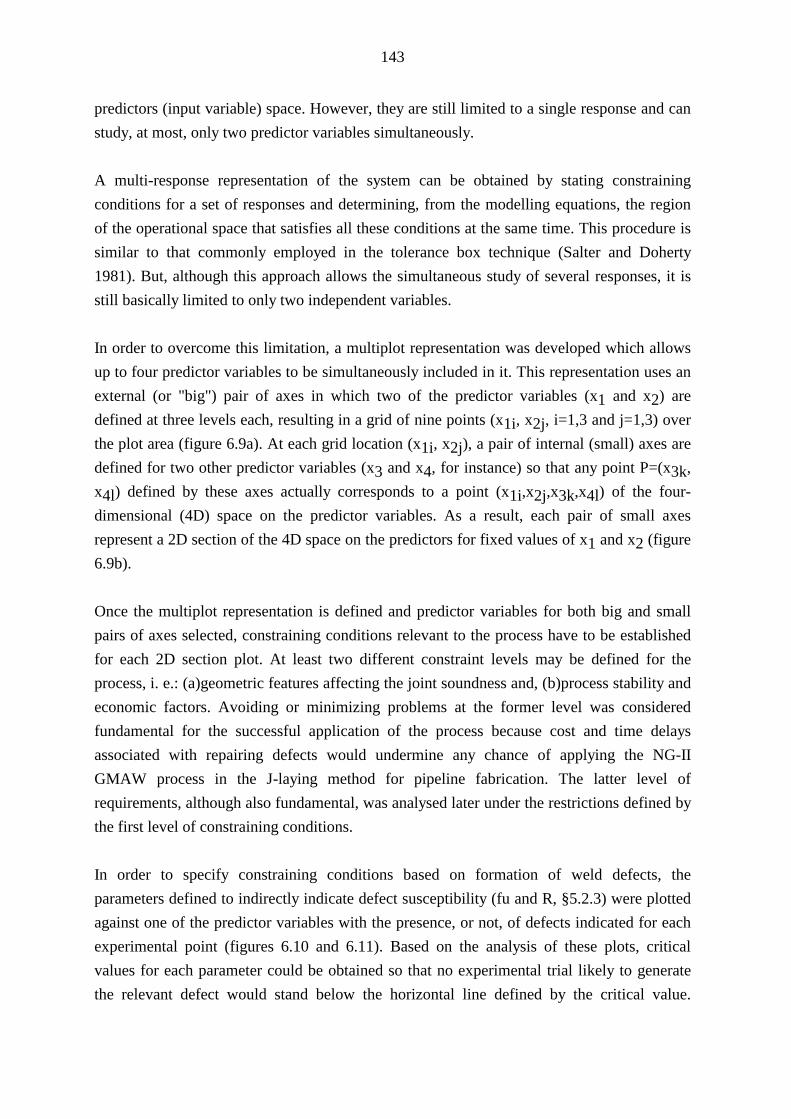
143
predictors (input variable) space. However, they are still limited to a single response and canstudy, at most, only two predictor variables simultaneously.
A multi-response representation of the system can be obtained by stating constrainingconditions for a set of responses and determining, from the modelling equations, the regionof the operational space that satisfies all these conditions at the same time. This procedure issimilar to that commonly employed in the tolerance box technique (Salter and Doherty1981). But, although this approach allows the simultaneous study of several responses, it isstill basically limited to only two independent variables.
In order to overcome this limitation, a multiplot representation was developed which allowsup to four predictor variables to be simultaneously included in it. This representation uses anexternal (or "big") pair of axes in which two of the predictor variables (x1 and x2) aredefined at three levels each, resulting in a grid of nine points (x1i, x2j, i=1,3 and j=1,3) overthe plot area (figure 6.9a). At each grid location (x1i, x2j), a pair of internal (small) axes aredefined for two other predictor variables (x3 and x4, for instance) so that any point P=(x3k,x4l) defined by these axes actually corresponds to a point (x1i,x2j,x3k,x4l) of the four-dimensional (4D) space on the predictor variables. As a result, each pair of small axesrepresent a 2D section of the 4D space on the predictors for fixed values of x1 and x2 (figure6.9b).
Once the multiplot representation is defined and predictor variables for both big and smallpairs of axes selected, constraining conditions relevant to the process have to be establishedfor each 2D section plot. At least two different constraint levels may be defined for theprocess, i. e.: (a)geometric features affecting the joint soundness and, (b)process stability andeconomic factors. Avoiding or minimizing problems at the former level was consideredfundamental for the successful application of the process because cost and time delaysassociated with repairing defects would undermine any chance of applying the NG-IIGMAW process in the J-laying method for pipeline fabrication. The latter level ofrequirements, although also fundamental, was analysed later under the restrictions defined bythe first level of constraining conditions.
In order to specify constraining conditions based on formation of weld defects, theparameters defined to indirectly indicate defect susceptibility (fu and R, §5.2.3) were plottedagainst one of the predictor variables with the presence, or not, of defects indicated for eachexperimental point (figures 6.10 and 6.11). Based on the analysis of these plots, criticalvalues for each parameter could be obtained so that no experimental trial likely to generatethe relevant defect would stand below the horizontal line defined by the critical value.
144
Critical values of 1.0 and 0.2 and valid for experimental blocks S1-B1, S1-B2 and S2-B1were defined by this criterion for R and fu respectively. This value for critical R issignificantly higher than values suggested for Kurokawa et al. (1966) who, however, workedwith much higher current levels and, consequently, a more massive weld pool. For lack offusion formation, the direct measured value of lack of fusion length in a bead cross sectionwas used to defined constraining levels. Negative values of lf, as defined in §5.2.3, were usedto indicate absence of fusion defects.
A nought value for lf could be an obvious initial candidate to critical value for fusion defectsensitivity. However, from a statistical point of view, this choice would actually imply that,although the expected value of lf was nought, there would be still a 50% chance that anexperimental trial, performed at that conditions, would generate a positive value of lf. Anapproach that is more conservative and also reproduces better the "pass-non-pass" criterionused for both cracking and undercutting determination would be:
yc = ytrans(lf = 0) - 2s [6.9]
where yc is the critical value for the transformed form of lf, ytrans (equation [2.35]), at lf = 0,and s is the estimated standard error of the transformed response.
This choice for the critical value corresponds approximately to a 4% chance that a positivevalue of lf would result from an experimental trial performed under conditions defined by yc.
Once critical levels for the responses considered relevant to the process are selected,estimated boundaries for adequate process operation can be obtained by setting the modellingequation for the given responses equal to their critical values, yc:
G( x1, x2, x3, x4) = yc [6.10]
Where G(...) is the modelling equation on predictors x1 to x4.
Using, for instance, x1 and x2 to define the two external axes, expression [6.10] can be easilysolved, if G is presented in the form of a model A or B type equation, for x3 and x4 in orderto define boundaries for expected defect formation at each location (x1i,x2j) of the externalgrid:
x4 = g(x1i,x2j, x3 , yc), i=1,3 and j=1,3 [6.11]
145
Lines for critical values of fu and lf considering wire feed rate and welding current as x3 andx4 respectively are shown in figures 6.12 to 6.14 for experimental steps S1-B1, S1-B2 andS2-B1. Each of these lines define a pair of values for x1 and x2, a boundary which dividesthe plotting area into two sub-regions of opposite characteristics regarding expectancy ofdefect presence. In one of the sub-regions, the restriction imposed by yc is not violated anddefect likelihood is small. On the other region, however, the restriction is not satisfied and itslikelihood is high. In figures 6.12 to 6.14, the former region for lf lies over its critical line (i.e., in the region of higher current and lower wire feed rate), while, for fu, it lies below itscritical line. In both cases, the critical lines tend to run diagonally with a positive slope closeto 45°.
Regions for expected defect-free operation are obtained by considering the critical lines forR, fu and lf together and finding, when it exists, the interception of the regions of acceptableoperation for each response. The resulting multiplots for experimental steps S1-B1 and S2-B1 are shown in figures 6.15 and 6.16. In these figures, the regions of expected defectabsence are represented by hatched areas.
A nought value for lf was used to define its critical boundary in figure 6.15 while a moreconservative limit, based on equation [6.9], was adopted in figure 6.16. The most extensiveregion of low defect likelihood was associated to experimental block S2-B1 (figure 6.16)with a 7mm gap width. This information was used to define operational conditions forhorizontal-vertical welding trials (block S3-B1). Results indicate that the process is highlysensitive to minor changes in input variables, including not only those used in the multiplotrepresentation but also other variables, such as wire positioning in the gap. Therefore,development of effective control systems may be a necessary requirement to the applicationof the process in production.
Finally, in both process representations, regions for adequate operation in terms of fusiondefects tend to extend diagonally in the (I,w) plane reflecting the role of arc length (orvoltage) in controlling lateral fusion. Mean slopes for these regions are approximately 0.05and 0.067 mA-1min-1 for S1-B1 and S2-B1 respectively. The reciprocals of the values areclose to (in absolute value) the parameter _I,w (table 6.3) for V and la indicating that, inthese regions, V and la should remain relatively constant. For instance, when the multiplotrepresentation for S1-B1 (figure 6.15) is compared with its surface plot for arc length (figure6.3a), a 3-4mm arc length seems to be associated with the region of adequate operation for an8mm gap and 8mm/s speed.
146
6.4.Horizontal-vertical welding
The weld beads of experimental block S3-B1 were basically free from undercutting andcentre line cracking problems. However, the conditions imposed on the weld pool byhorizontal-vertical (HV) position resulted in a non-uniform fusion of the workpiece, with itslower face presenting much less fusion than the upper face (figure 5.7).
Compared with previous results for the downhand position, the modelling equation for lateralpenetration area (including fusion in both upper and lower walls) indicated only weldingspeed to be significant (figure 6.17). Neither current nor wire feed rate seem to have asignificant effect for the experimental conditions employed. As a result, arc length alsoseems to have little effect. This result was rather unexpected when compared with previousexperimental blocks and may be partially linked to the short arc conditions that wereintentionally used in this experimental block once a high tendency to undercutting in theupper wall was initially expected. These conditions together with the gravity influence on theHV position may have forced the arc to burn almost completely under the joint bottom.
The non-uniform characteristic of the arc lateral fusion in the HV position is clearly shownwhen the individual values of upper and lower side wall fusion areas are compared (figure6.18). The ratio between fused area in the upper and lower walls:
RUL = Apu/Apl [6.12]
can be taken as a measure of the arc relative efficiency to melt the upper and lower walls.Mean values, at constant welding speed, for RUL are presented in table 6.4 together withother parameters related with bead asymmetry. Results indicate that, for welding speedsequal or below 8mm/s, a fivefold difference in fusion is commonly present. For higherwelding speeds, the relative advantage of upper side wall in melting efficiency is reducedmainly by a faster decrease in lateral fusion in this wall.
Lack of fusion behaviour in the HV position also indicates unequal arc melting efficiency(table 6.4). Under the welding conditions used in the experimental block, large negativevalues of lf were common for the upper side wall while, in the lower side, extensive lack offusion could be found. However, values indicated for lfl may be overestimated by somemargin due to the different methodology used to define lack of fusion in the lower wall(figure 5.8).
147
One further feature related with lateral fusion in the HV position is a tendency for hmax(figure 5.4) to be longer in the upper wall. As a result, the weld face tended to be inclined inrelation to the side walls and a sharp corner may be formed between the weld face and thelower side wall. If this sharp corner is formed, the likelihood of fusion defect formation inthis area is greatly increased for the next run. The difference between hmax in upper andlower walls respectively is commonly over 25% for welding speeds up to 8mm/s (table 6.4).
Higher fusion in the upper part of the joint is also demonstrated by the axial penetration areawhich has an asymmetrical character as shown by the values of the ratio between the upperand lower halves of Aa (RALU, figure 6.19). A surface plot for Aa in block S3-B1 ispresented in figure 6.17.
Hence, the most striking feature of the NGW process in the HV position is the asymmetricalcharacter of workpiece fusion, particularly in the side walls. Similar results were observed byFoote (1986) who related them to sagging of the weld pool which shielded the bottom face ofthe joint from direct heating by the arc. In order to study this effect and to analyse otheraspects of bead formation, Foote (1986) developed a simplified model for weld pool saggingin H-V position following closely the work of Berozovski et al. (1983) and Nishiguchi et al.(1978). In this model, the balance between gravity and surface tension forces was consideredon a two dimensional static pool where arc force was considered negligible (see §2.4.2.1).Areas of undercutting and sagging were defined and regions of adequate bead formationfound provided that the gap (bead) width was under about 12mm. However, this model doesnot consider the influence of the arc and can only be possibly applied to conditions found atthe rear part of the weld pool. It is, therefore, doubtful that this model could analysedifferential plate fusion in HV-NG welding which is probably more related to the interactionbetween gravity and arc force in the weld pool. In this situation, a layer of liquid metal wouldbe forced by the combined action of the plasma jet and gravity to the bottom side of the joint,shielding this area from a more direct arc action (figure 6.20).
Therefore, asymmetrical plate fusion should be controlled, or at least reduced, by forcing anincreased arc action on the lower side of the joint by, for instance, reducing gap width orwelding with the wire positioned below the joint centreline. Complementary welding trials(table 5.8) demonstrated the effect of gap width in both axial and lateral fusion and lack offusion tendency for H-V welding. Results indicate that a reduction of just 1mm in gap widthcan alter significantly fusion levels (figures 6.21 to 6.23). One further complementary trialwas performed employing reduced gap width and off-centre wire positioning in a taperedjoint preparation (figure 6.24). Figure 5.10b presents a macrograph of the multi-pass weldedspecimen. Improved bottom fusion can be observed with no indication of fusion defects.
148
Fusion characteristics may have been also improved by a lower wire feed rate which wouldtend to produce a longer arc.
Although experimental results have shown that plate fusion is significantly affected bywelding position, the modelling equation for bead area in block S3-B1 is quite similar tothose obtained for other experimental blocks.
6.5.Summary
Statistical modelling techniques such as those used in this programme provide powerful toolsfor designing and running a experimental programme of a industrial nature, analysing itsresults and building empirical models. These techniques do not, however, substitute a systemfor the expertise that may be available, and, if not employed effectively, misleading andconfusing results may be obtained.
The results of the experimental blocks welded in the downhand position are in good generalagreement with previous studies. In addition to traditional parameters, such as weldingcurrent, speed and, in special, gap width, the importance of other parameters, particularly theoptimisation of in shielding gas composition and power supply characteristics, wasdemonstrated. A multiplot representation of process operation was developed to study thesimultaneous effect of up to four input variables. It demonstrated that acceptable weldingconditions in terms of preventing fusion defects are linked to an approximately constant arclength.
Asymmetrical lateral fusion was the main characteristic of H-V welding operation. Thischaracteristic was related to the combined action of gravity and arc force and, in order tominimize its effects, a narrower gap width and off-centre wire positioning were used.
In general, the results suggested conditions for obtaining welded joints free from fusiondefects and with welding times compatible with the J-laying method. However, it alsodemonstrated that the process is rather sensitive to minor changes in welding parameters andthe development of adequate control system is expected to be a necessary step to itsapplication in a real production situation.
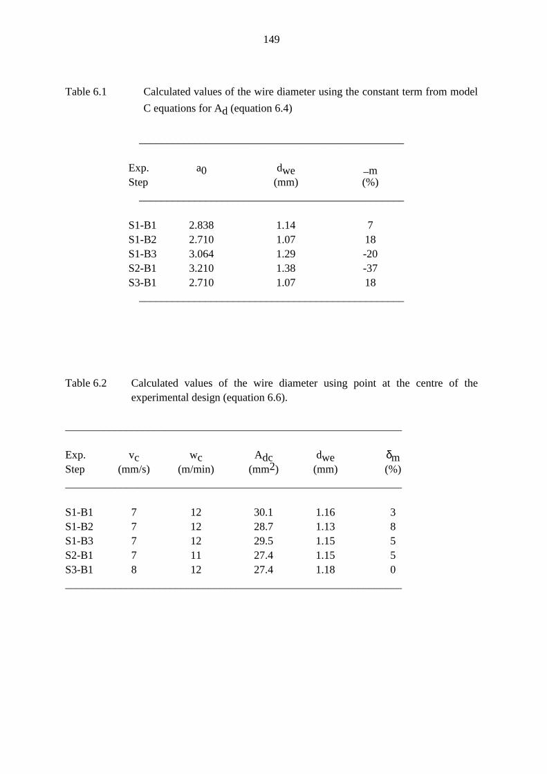
149
Table 6.1 Calculated values of the wire diameter using the constant term from modelC equations for Ad (equation 6.4)
________________________________________________
Exp. a0 dwe _mStep (mm) (%)
________________________________________________
S1-B1 2.838 1.14 7S1-B2 2.710 1.07 18S1-B3 3.064 1.29 -20S2-B1 3.210 1.38 -37S3-B1 2.710 1.07 18
________________________________________________
Table 6.2 Calculated values of the wire diameter using point at the centre of theexperimental design (equation 6.6).
_____________________________________________________________
Exp. vc wc Adc dwe δmStep (mm/s) (m/min) (mm2) (mm) (%)_____________________________________________________________
S1-B1 7 12 30.1 1.16 3S1-B2 7 12 28.7 1.13 8S1-B3 7 12 29.5 1.15 5S2-B1 7 11 27.4 1.15 5S3-B1 8 12 27.4 1.18 0_____________________________________________________________
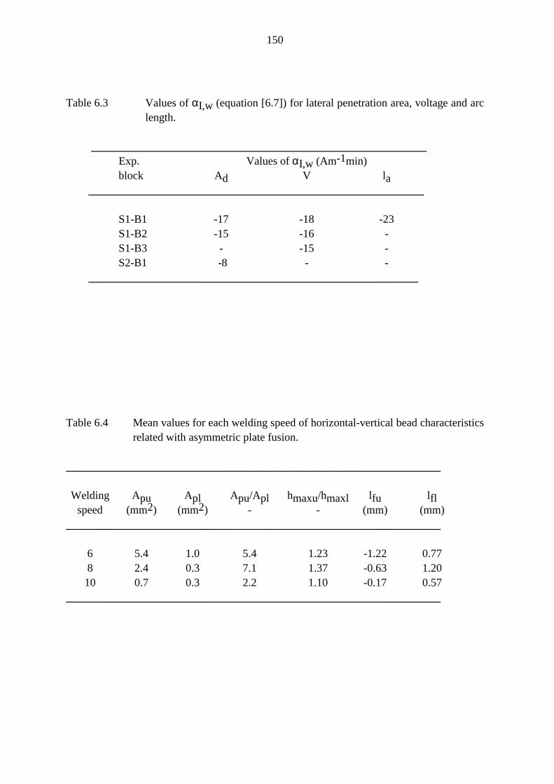
150
Table 6.3 Values of αI,w (equation [6.7]) for lateral penetration area, voltage and arclength.
____________________________________________________________Exp. Values of αI,w (Am-1min)block Ad V la
____________________________________________________________
S1-B1 -17 -18 -23S1-B2 -15 -16 -S1-B3 - -15 -S2-B1 -8 - -
___________________________________________________________
Table 6.4 Mean values for each welding speed of horizontal-vertical bead characteristicsrelated with asymmetric plate fusion.
___________________________________________________________________
Welding Apu Apl Apu/Apl hmaxu/hmaxl lfu lflspeed (mm2) (mm2) - - (mm) (mm)
___________________________________________________________________
6 5.4 1.0 5.4 1.23 -1.22 0.778 2.4 0.3 7.1 1.37 -0.63 1.2010 0.7 0.3 2.2 1.10 -0.17 0.57
___________________________________________________________________
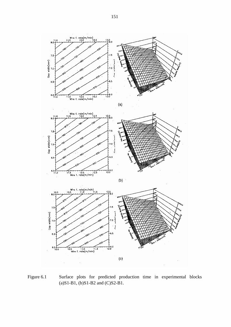
151
Figure 6.1 Surface plots for predicted production time in experimental blocks(a)S1-B1, (b)S1-B2 and (C)S2-B1.
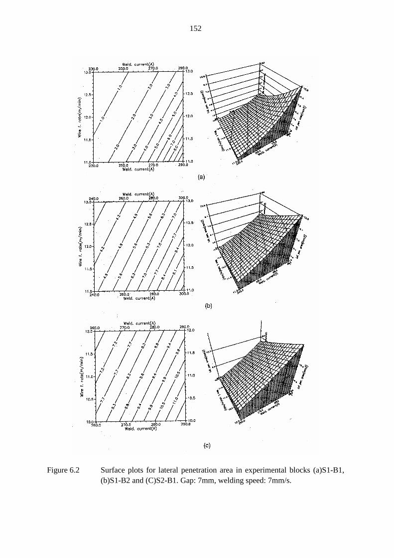
152
Figure 6.2 Surface plots for lateral penetration area in experimental blocks (a)S1-B1,(b)S1-B2 and (C)S2-B1. Gap: 7mm, welding speed: 7mm/s.
153
Figure 6.3 Surface plots for predicted (a)voltage and (b)arc length in experimentalblock S1-B1.
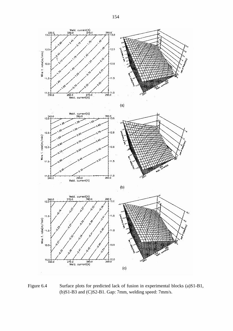
154
Figure 6.4 Surface plots for predicted lack of fusion in experimental blocks (a)S1-B1,(b)S1-B3 and (C)S2-B1. Gap: 7mm, welding speed: 7mm/s.
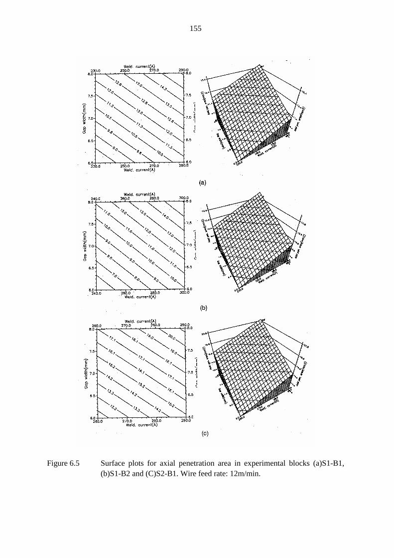
155
Figure 6.5 Surface plots for axial penetration area in experimental blocks (a)S1-B1,(b)S1-B2 and (C)S2-B1. Wire feed rate: 12m/min.
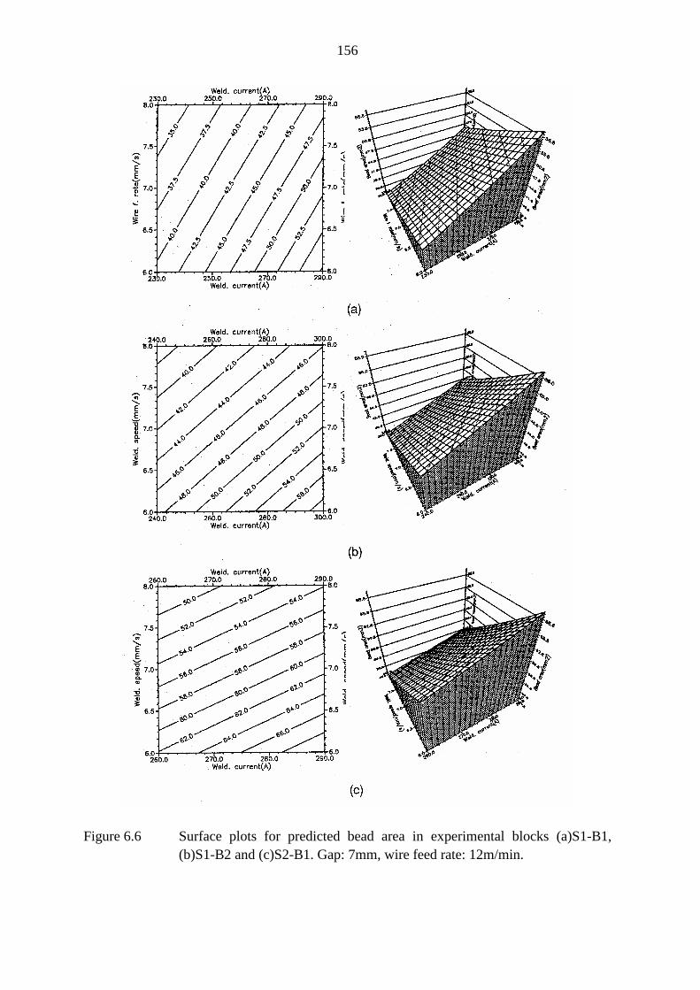
156
Figure 6.6 Surface plots for predicted bead area in experimental blocks (a)S1-B1,(b)S1-B2 and (c)S2-B1. Gap: 7mm, wire feed rate: 12m/min.
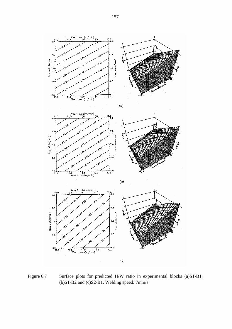
157
Figure 6.7 Surface plots for predicted H/W ratio in experimental blocks (a)S1-B1,(b)S1-B2 and (c)S2-B1. Welding speed: 7mm/s
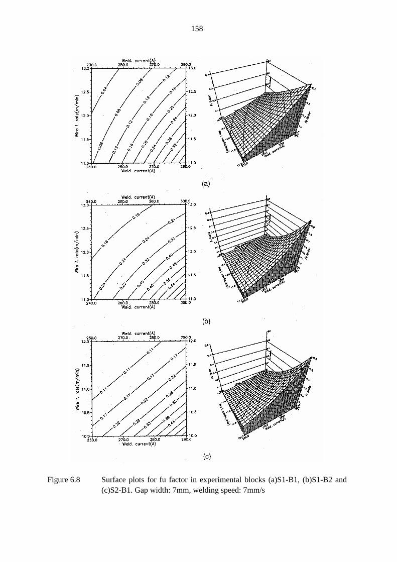
158
Figure 6.8 Surface plots for fu factor in experimental blocks (a)S1-B1, (b)S1-B2 and(c)S2-B1. Gap width: 7mm, welding speed: 7mm/s
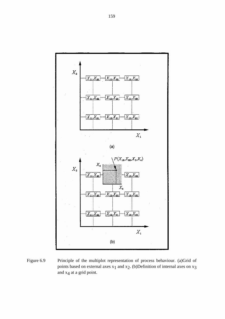
159
Figure 6.9 Principle of the multiplot representation of process behaviour. (a)Grid ofpoints based on external axes x1 and x2. (b)Definition of internal axes on x3and x4 at a grid point.
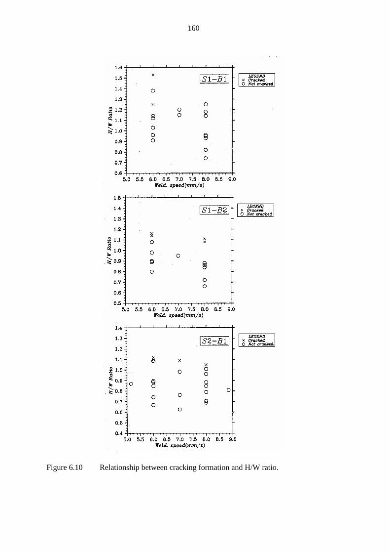
160
Figure 6.10 Relationship between cracking formation and H/W ratio.
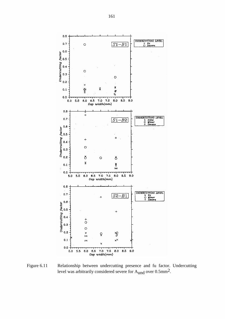
161
Figure 6.11 Relationship between undercutting presence and fu factor. Undercuttinglevel was arbitrarily considered severe for Aund over 0.5mm2.
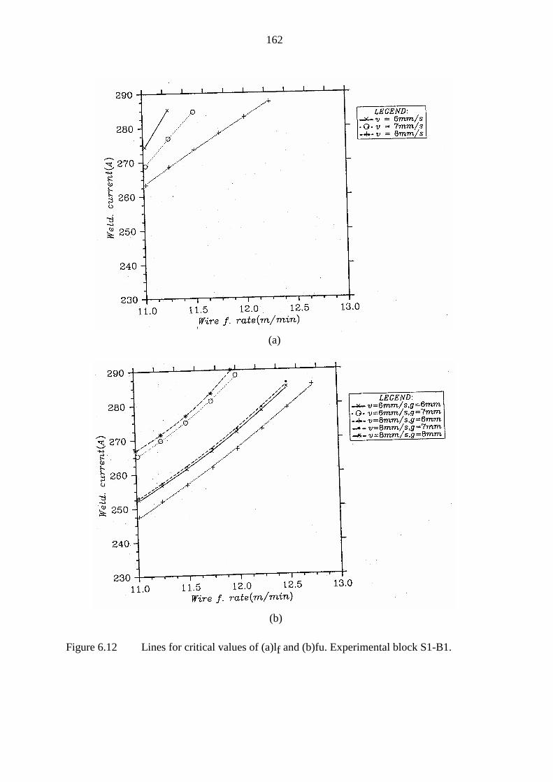
162
(a)
(b)
Figure 6.12 Lines for critical values of (a)lf and (b)fu. Experimental block S1-B1.
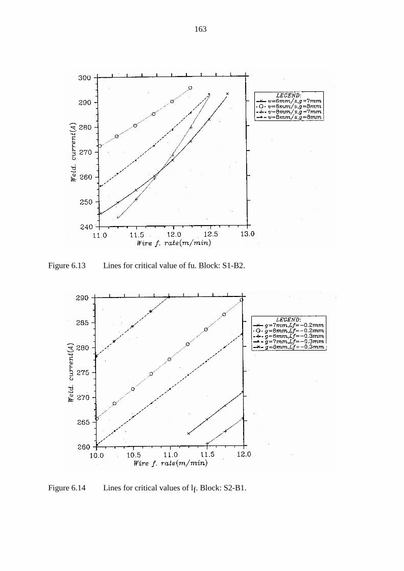
163
Figure 6.13 Lines for critical value of fu. Block: S1-B2.
Figure 6.14 Lines for critical values of lf. Block: S2-B1.
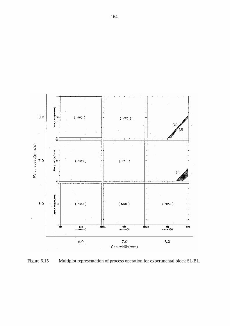
164
Figure 6.15 Multiplot representation of process operation for experimental block S1-B1.
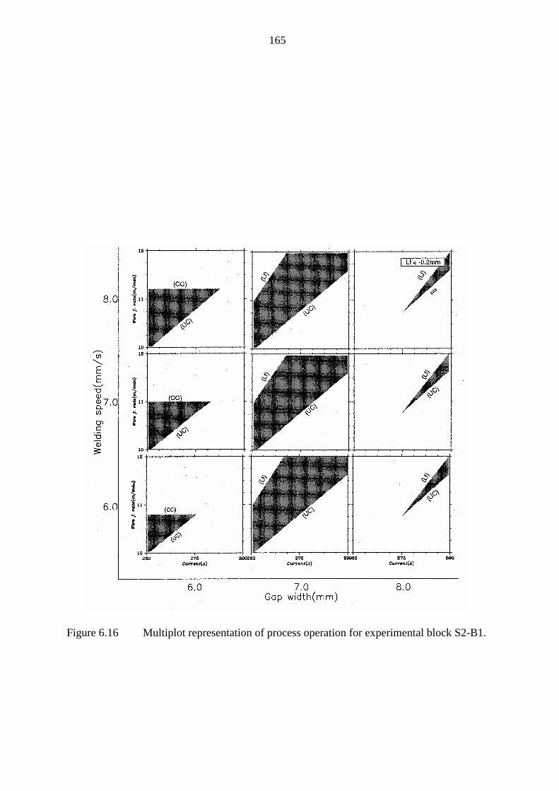
165
Figure 6.16 Multiplot representation of process operation for experimental block S2-B1.
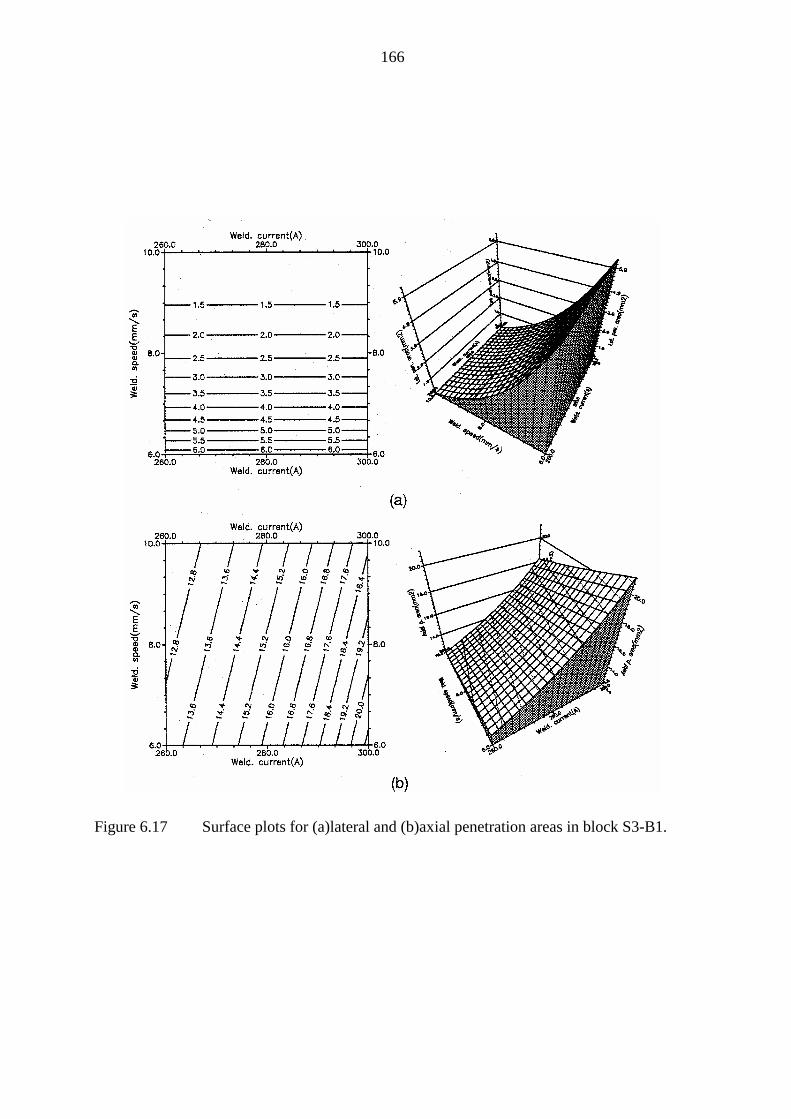
166
Figure 6.17 Surface plots for (a)lateral and (b)axial penetration areas in block S3-B1.
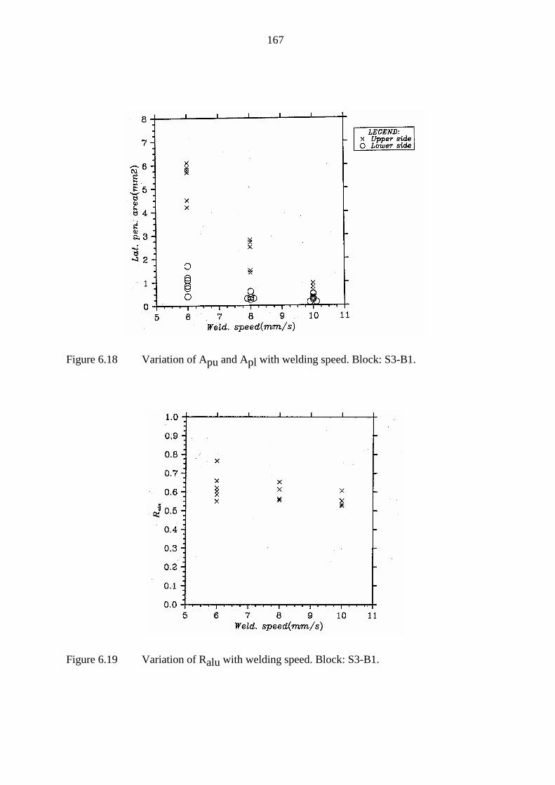
167
Figure 6.18 Variation of Apu and Apl with welding speed. Block: S3-B1.
Figure 6.19 Variation of Ralu with welding speed. Block: S3-B1.
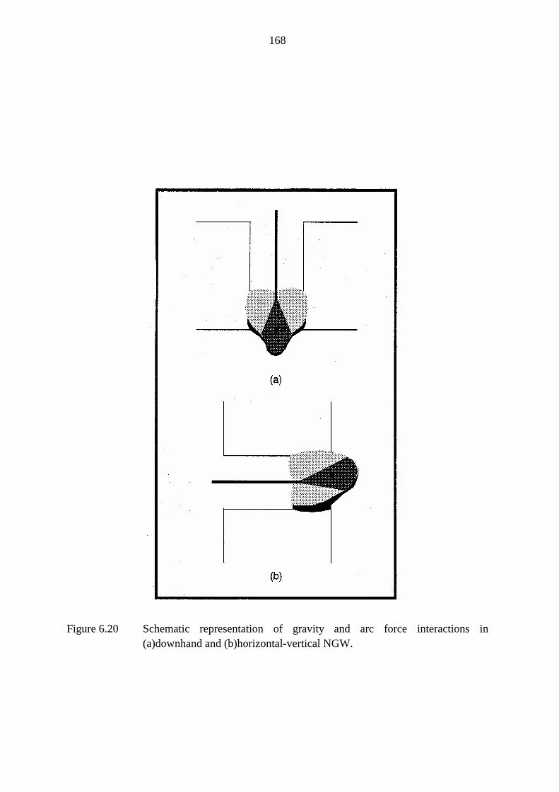
168
Figure 6.20 Schematic representation of gravity and arc force interactions in(a)downhand and (b)horizontal-vertical NGW.
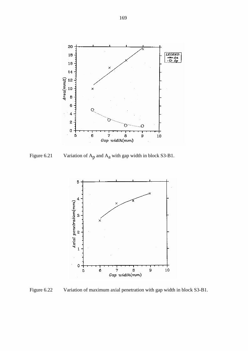
169
Figure 6.21 Variation of Ap and Aa with gap width in block S3-B1.
Figure 6.22 Variation of maximum axial penetration with gap width in block S3-B1.
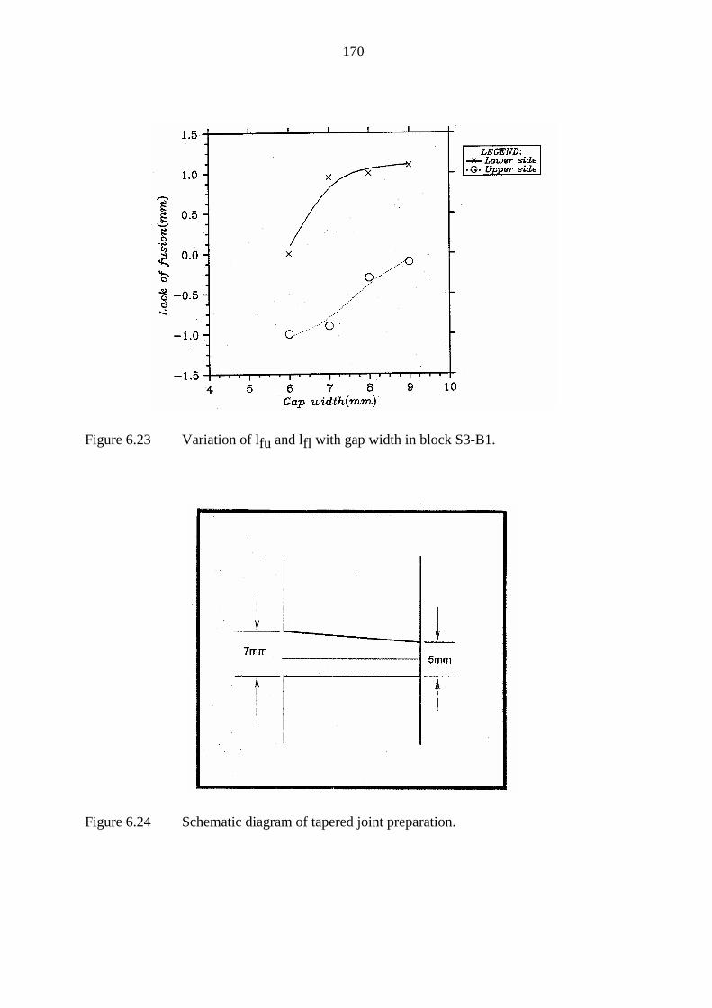
170
Figure 6.23 Variation of lfu and lfl with gap width in block S3-B1.
Figure 6.24 Schematic diagram of tapered joint preparation.

CHAPTER 7
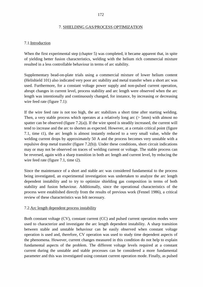
172
7. SHIELDING GAS/PROCESS OPTIMIZATION
7.1.Introduction
When the first experimental step (chapter 5) was completed, it became apparent that, in spiteof yielding better fusion characteristics, welding with the helium rich commercial mixtureresulted in a less controllable behaviour in terms of arc stability.
Supplementary bead-on-plate trials using a commercial mixture of lower helium content(Helishield 101) also indicated very poor arc stability and metal transfer when a short arc wasused. Furthermore, for a constant voltage power supply and non-pulsed current operation,abrupt changes in current level, process stability and arc length were observed when the arclength was intentionally and continuously changed, for instance, by increasing or decreasingwire feed rate (figure 7.1):
If the wire feed rate is not too high, the arc stabilizes a short time after starting welding.Then, a very stable process which operates at a relatively long arc (> 5mm) with almost nospatter can be observed (figure 7.2(a)). If the wire speed is steadily increased, the current willtend to increase and the arc to shorten as expected. However, at a certain critical point (figure7.1, time t1), the arc length is almost instantly reduced to a very small value, while thewelding current drops by approximately 50 A and the process becomes very unstable with arepulsive drop metal transfer (figure 7.2(b)). Under these conditions, short circuit indicationsmay or may not be observed on traces of welding current or voltage. The stable process canbe reversed, again with a sharp transition in both arc length and current level, by reducing thewire feed rate (figure 7.1, time t2).
Since the maintenance of a short and stable arc was considered fundamental to the processbeing investigated, an experimental investigation was undertaken to analyze the arc lengthdependent instability and to try to optimize shielding gas composition in terms of bothstability and fusion behaviour. Additionally, since the operational characteristics of theprocess were established directly from the results of previous work (Fennel 1986), a criticalreview of these characteristics was felt necessary.
7.2.Arc length dependent process instability
Both constant voltage (CV), constant current (CC) and pulsed current operation modes wereused to characterize and investigate the arc length dependent instability. A sharp transitionbetween stable and unstable behaviour can be easily observed when constant voltageoperation is used and, therefore, CV operation was used to study time dependent aspects ofthe phenomena. However, current changes measured in this condition do not help to explainfundamental aspects of the problem. The different voltage levels required at a constantcurrent during the unstable and stable processes can be considered a more fundamentalparameter and this was investigated using constant current operation mode. Finally, as pulsed
173
current was used in experimental step S1, some tests were performed to characterize theproblem in this operational mode.
7.2.1.Initial experiments
A preliminary series of bead-on-plate tests was carried out in order to determine some initialcharacteristics of the instability phenomena. Variable wire feed rate trials (see previoussection and figure 7.1) were performed with Helishield 101, argon and Argoshield 5. Resultsindicated that clear transition points could be observed when either He-101 or Ar were usedbut not with Ar-5.
In order to characterize the instability phenomena under constant current operation, a set oftrials was carried out using sloped specimens (figure 7.3) which resulted in a continuousreduction in standoff distance during the welding trial. Argon and Ar-1%O2 were used forshielding. Instead of presenting a sharp transition, as observed with constant voltage, theprocess stability tended to continuously deteriorate as the standoff was shortened. A largenumber of spikes appeared in the voltage trace at the same time as stability deteriorates.However, instead of presenting a definitive step from one state to the order, the voltage tracesseemed to indicate a continuous transition.
7.2.2.Tests with constant voltage
Bead-on-plate welding trials were performed with the Fronius TPS-500 power supply inconstant voltage operation. Each welding trial was started using a low voltage setting (=shortarc) in order to force the process to operate initially in the unstable mode. After a short while,the voltage was rapidly increased to its test value and the welding operation continued untilthe process behaviour changed. This transition in behaviour was marked in the weldingcurrent trace by a sudden current increase (figure 7.4). A logging time interval of between 20and 40 ms was used in the VELA to record the current trace. Logging times of thismagnitude provided a total measuring time of 20-40s which was long enough in most casesto detect the transition in behaviour while keeping a satisfactory resolution (in time) to detectthe instant of transition. The time necessary for the process to change its operationalcharacteristics (ts = t1-t0, figure 7.4) was measured from current and voltage traces. Pureargon, Helishield 101 and mixtures of either gas with oxygen were used as shielding gases.
The results of the process stability tests with CV operation are presented in table 7.1 andfigure 7.5. Despite a relatively large spread of the results, a clear tendency towards shortertransitions times for both higher oxygen content and arc voltage can be noticed.
The transition from unstable to stable operational mode (and vice versa) is quite remarkablefor CV operation. Abrupt changes in current level and arc length take place during thistransition. Current level differences of 40-90A were found while high-speed photographs by
174
the IMACON camera suggested a variation in arc length from 0-1mm during unstableoperation to 7-8mm in stable operation (figure 7.6). At the same time, metal transfer alsochanges from a repulsive globular mode to spray. For all shielding gases but pure argon, theprocess did not tend to revert back into unstable operation once it has changed into the stablemode. For pure argon shielding, the process occasionally reverted back to unstable operationwith the arc length shortening abruptly and apparently stubbing into the workpiece.
7.2.3.Tests with constant current
An extensive experimental programme was undertaken with constant current operation. Fiveshielding gas compositions were investigated: argon, Ar-25%He, Ar-75%He, helium andAr-2%O2. As the main objectives of these tests was to analyze the voltage levels associatedwith both the stable and unstable processes, most of the experimental trials were performedusing pure inert gas shielding which was expected to promote the unstable processoccurrence. The Ar-2%O2 mixture was used to study the effect of oxygen on the processbehaviour. Bead-on-plate welding trials with different standoff distances, wire feed rates andcurrent levels were performed (table 7.2). No arc length measurements were performed in theexperiment. However, considering the relative independence of wire melting rate from bothshielding gas composition and arc length (Lesnewich 1958a and Nunes 1982), anapproximately direct relationship between standoff distance and arc length can be assumed.In most of the trials, the ordinary experimental system with the GEC (AWP) M500 powersupply was used. A few trials, however, were performed inside a hyperbaric chamber whichwas previously evacuated and then filled with shielding gas (argon) at atmospheric pressure.As the transitions in process behaviour tended to be much faster under CC operation than CVoperation, a logging time of 1 ms was used to record the arc voltage traces.
In behaviour similar to the results reported in the previous section, process stability wasworse for shorter arc (or shorter standoff distance) welding operation. Voltage traces fordifferent gas compositions, current and standoff values are shown in figures 7.7 to 7.10. Ifthe shielding gas contained argon and the arc length was sufficiently long, a stable spray arccould be formed (figure 7.11) and the voltage trace was relatively featureless. Shorter arcoperation resulted in lower stability and a higher spatter level. Again, when the shielding gascontained argon, three characteristic voltage levels could be observed: (a)short circuitvoltage, V0, (b)intermediate arc voltage level, Vst, and (c)high voltage level, Vuns (figure7.12). Two very distinct metal transfer/arc modes seem to operate in this condition (figure7.13). These appear to be similar to those observed in the previous section apart from thechange in arc length that was associated with the CV characteristic and did not seem to takeplace in CC operation.
When pure helium was used for shielding, metal transfer tended always to be globularregardless of arc length. Although, no clearly distinct arc voltage levels could be observed,the voltage trace tended to be more irregular for short arc operation.
175
The voltage distribution from traces of different experimental conditions is shown byfrequency polygon plots in figures 7.14 to 7.22. These plots were prepared by dividing thevoltage range into an arbitrary number of intervals and counting the number of data pointsthat were included in each interval. The presence of more than one peak of voltage in someof these plots is due to the different voltage levels of the process. Table 7.3 presents themeasured values of Vuns and Vst.
Vuns and Vst tend to increase with standoff distance and helium content in the shielding gas(figures 7.23 and 7.24). The mean value of the difference between Vuns and Vst, however,decreased with helium content and also with welding current (figure 7.25). On the otherhand, oxygen addition caused an increase in (Vuns-Vst), mainly by dropping Vst (compareplots for pure Ar and Ar-2%O2, figure 7.23).
7.2.4.Tests with pulsed current
Bead-on-plate welds were deposited using He-1 or He-2 gas mixtures with different oxygenadditions and wire feed rates. The Fronius TPS500 power supply was used in pulsed CVCCmode. The current trace was recorded with a logging time of 0.100 ms, a few seconds afterthe stabilization of welding conditions. The resulting data files were processed and the pulsedcurrent parameters measured (table 7.4).
A trend similar to that of the previous sections was also detected with CVCC pulsed currentoperation. Particularly, a transition from a condition characterized by spray transfer and astable and quiet arc to one dominated by unstable repulsive metal transfer was observedwhen the arc was shortened. The arc length seemed to change during the transition but not asclearly as with CV operation. One initial difficulty was to define a parameter to characterizethe instability process in pulsed current. Both mean voltage and current tended to fluctuatemore strongly during unstable behaviour but a clear tendency was not observed. However,test results indicated that a good correlation between process behaviour and the standarddeviation of the peak current could be attained. Consequently, this parameter was selected toquantify the arc length dependent process instability under pulsed current (CVCC) operation.
The influence of wire feed rate and oxygen content in the gas on the process stabilitymeasured by the standard deviation of peak current (sp) is shown in figure 7.26. This figureindicates that the unstable operation, which is associated with a value of sp over 20A, tendsto predominate for short arc operation (i. e., for high wire feed rate) and a low oxidizingpotential of the shielding gas.
The current trace from bead-on-plate and narrow gap welding performed with differenthelium contents in the shielding gas (§7.3, table 7.5) was also studied to evaluate the effectof helium content in process stability (table 7.6 and figure 7.27).
176
7.3.Fusion characteristics
In order to study the effect of the helium content in Ar-He-2%O2 mixtures on weld beadcharacteristics, bead-on-plate and narrow gap specimens were welded with different gascompositions (table 7.5). The trials were carried out using pulsed current (CVCC mode). Thevalue of the welding current was recorded with a logging time magnitude of 0.100ms andused to calculate the pulse characteristics (table 7.6). Two transverse macrographs wereprepared from each welded specimen and the bead geometric parameters measured fromthem (figure 7.28 and 7.29). The weld bead geometric parameters defined in §5.2.3 weremeasured in the narrow gap specimens. Similar parameters were used for bead-on-platespecimens (figure 7.30). Furthermore, dilution (δ) and penetration factor (fp) were alsomeasured to indicate plate fusion tendencies. Dilution was defined as usual:
δ = Aa/(Aa + Ad) = Aa/At [7.1]
while fp was defined as:
fp = 100.(p1 + p2)/pmax [7.2]
where p1, p2 and pmax are shown in figure 7.30.
The measured bead parameters are presented in table 7.7. The influence of the heliumcontent in the shielding on some bead characteristics for both narrow gap and bead-on-plateis shown in figures 7.31 and 7.32. It was found that axial penetration area in both NG andBOP welding trials and lateral penetration area in NGW trials increased with %He in theshielding. This increase was mainly associated with the secondary penetration while thefinger penetration (pmax) remained approximately constant at around 3.5mm for the bead-on-plate trials performed with the shielding gases that contained helium. The increase infused area (Aa or Ap) results also in an improvement in dilution and penetration factor.There is a clear tendency for bead area to be greater in BOP than NG welding under similarconditions. A difference of around 10% between BOP and NG bead areas was found for theshielding gases containing He, independently of its actual content. Under Ar-O2 shielding, aslightly higher difference (15%) was obtained. This difference resulted mainly from areduction in Aa in NGW which was not entirely compensated by lateral fusion of the sidewalls. This may be explaining by the confining effect of the groove walls which wouldincrease the weld pool height and make it more difficult for the arc to reach the base metal atthe bottom of the joint. The results also indicated a tendency for deposited area be slightlysmaller in welding trials with higher helium contents for both BOP and NG welding. Finally,bead width in BOP welding and mean bead height and H/W ratio in NGW were notsignificantly affected by gas composition.
177
7.4.Power supply characteristics
In spite of the enormous recent progress in process control and power supply electronics,constant voltage operation is still quite popular mainly due to its simple and effective self-adjusting arc capability (§2.2.6.2). However, this characteristic is strictly operative only forbead-on-plate welding or a similar geometric arrangement. Under these conditions and if thestandoff distance is kept constant, any small variation in arc length is compensated by anopposite variation in stickout, i. e.:
h = s + la, and [5.1]
d(la) = -d(s) [7.3]
Inside a narrow gap joint, two extreme conditions can be defined:
. If the arc is short enough, it will root mainly on the bottom of the joint and the weldpool edges. The resulting system will respond to small perturbations similarly tobead-on-plate welding (figure 7.33a).
. If the arc becomes too long, it will tend to deflect to the joint sidewalls and notreach the bottom of the joint. In this situation, the arc length will remain essentiallyconstant and independent of the stickout (figure 7.33b):
d(la) = 0 [7.4]
Intermediate conditions should prevail for operative conditions between these two extremes.
To investigate the response of the GMAW system to small perturbations, the summation ofvoltage drops around the current loop is considered (figure 7.34):
V = Varc + Vs [7.5]
Where V is the mean voltage provided by the power supply and measured between theworkpiece and the torch contact tip, Varc is the arc voltage, and Vs is the voltage drop along the electrode stickout.
For small variations the arc voltage can be considered independent of current and berepresented approximately by equation [2.2]:
Varc = Va + Vc + Ela [2.2]
The voltage drop in the electrode stickout is difficult to quantify because of the complextemperature profile in the stickout. However, the effective wire resistivity (_) can be
178
considered approximately independent of the welding current (Lund 1979 and Waszink andvan den Heuvel 1979). This assumption can be considered valid particularly if the study isrestricted to only small perturbations of the system about an established operating point. Theresulting expression for the voltage drop in the stickout is therefore:
[7.6]Vs = (τ/Aw)sI [7.6]
Substituting [2.2] and [7.6] in equation [7.5] and taking the derivative results:
d(V) = (τ/Aw)s.d(I) + (τ/Aw)I.d(s) + Ed(la) [7.7]
In bead-on-plate welding, if the standoff distance is kept constant, relation [7.3] can beapplied. For constant voltage operation, the power supply characteristic can be representedby:
V = V0 - RI [7.8]
where V0 is the open circuit voltage, and R is a resistive term linked to the power supply slope. Therefore:
-Rd(I) ≈ (τ/Aw)s.d(I) - (τ/Aw)I.d(la) + Ed(la), or:
( )))(/(
/
aw
w
a lhAREIA
dldI
−+−
=ττ
[7.9a]
Where R [V/A] is the power supply slope.
Considering, for a 1.2mm mild steel wire and a welding current of 300A, τ/Aw ≈ 1 Ω/m,based on its electrical resistivity at approximately 800°C (ASM 1978), R = 1V/100A and E =800 V/m (Allum 1986), the derivative in [7.9a] will be equal to (in A/m):
)()21(500
aa lhEdldI
−+−= [7.9b]
The negative value for the derivative in [7.9] just expresses the arc self-regulating capabilityin CV operation, i. e., the opposite direction of change for welding current and arc length. InCC operation, d(I) = 0 and:
mVIAEsd
dVdldV
wa
/500)/( ≈−≈−= τ [7.10]
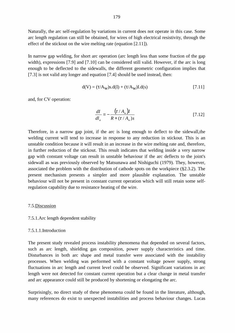
179
Naturally, the arc self-regulation by variations in current does not operate in this case. Somearc length regulation can still be obtained, for wires of high electrical resistivity, through theeffect of the stickout on the wire melting rate (equation [2.11]).
In narrow gap welding, for short arc operation (arc length less than some fraction of the gapwidth), expressions [7.9] and [7.10] can be considered still valid. However, if the arc is longenough to be deflected to the sidewalls, the different geometric configuration implies that[7.3] is not valid any longer and equation [7.4] should be used instead, then:
d(V) = (τ/Aw)s.d(I) + (τ/Aw)I.d(s) [7.11]
and, for CV operation:
( )sAR
IAdldI
w
w
a )/(/τ
τ+
−= [7.12]
Therefore, in a narrow gap joint, if the arc is long enough to deflect to the sidewall,thewelding current will tend to increase in response to any reduction in stickout. This is anunstable condition because it will result in an increase in the wire melting rate and, therefore,in further reduction of the stickout. This result indicates that welding inside a very narrowgap with constant voltage can result in unstable behaviour if the arc deflects to the joint'ssidewall as was previously observed by Matsunawa and Nishiguchi (1979). They, however,associated the problem with the distribution of cathode spots on the workpiece (§2.3.2). Thepresent mechanism presents a simpler and more plausible explanation. The unstablebehaviour will not be present in constant current operation which will still retain some self-regulation capability due to resistance heating of the wire.
7.5.Discussion
7.5.1.Arc length dependent stability
7.5.1.1.Introduction
The present study revealed process instability phenomena that depended on several factors,such as arc length, shielding gas composition, power supply characteristics and time.Disturbances in both arc shape and metal transfer were associated with the instabilityprocesses. When welding was performed with a constant voltage power supply, strongfluctuations in arc length and current level could be observed. Significant variations in arclength were not detected for constant current operation but a clear change in metal transferand arc appearance could still be produced by shortening or elongating the arc.
Surprisingly, no direct study of these phenomena could be found in the literature, although,many references do exist to unexpected instabilities and process behaviour changes. Lucas
180
and Amin (1975) assigned alterations in metal transfer to the deoxidation level of GMAWsteel wires of the same grade. Exploding drop transfer was associated with high oxygenlevels in the wire whilst stream spray transfer predominated for low oxygen levels. Noinfluence of shielding gas composition could, however, be found. In a paper studying arcstabilization by rare earth additions, Agusa et al. (1981) mention unstable operation withperiodic spray transfer and wire stubbing in the welding of mild steel under pure argonshielding. Scale on the plate surface could prevent wire stubbing. Kiyohara et al. (1977 and1979) linked changes in drop size and wire melting rate in the spray GMAW of aluminumwith arc length. Rodwell (1985) studied arc disturbances and variable weld bead shape in thespray GMAW of stainless and mild steels. Sudden and violent changes in arc length andcurrent level were associated with contamination on the wire surface and contact tip wear.Middleton (1988) observed an unexpected increase in voltage at short arc lengths duringdevelopment of an arc-voltage-control system for the GMA welding of Inconel with constantcurrent. Though this phenomenon resulted in the abandonment of the project, no furtherstudy of it was performed. Foote (1986) observed arc instability in bead-on-plate GMAWtrials with Helishield 1 and certain wire compositions. A paper from Hazlett and Gordon(1957) shows welding current traces that present abrupt and unexpected changes in currentlevel. However, no comment regarding this behaviour was made.
The present work has demonstrated the existence of an arc stability problem which waslinked to shielding gases of low oxidising potential and short arc operation. Although oxygenlevel in the shielding is generally kept high enough to prevent this instability problem duringthe welding of mild or low alloy steels, completely inert shielding is necessary for most ofthe nonferrous alloys and a low oxidizing one can be advantageous for the welding of highalloy steels. The unstable behaviour was first observed in narrow gap welding trials withHe-1 and, later, in bead-on-plate welding with He-101. Both of these commercial Ar-Heshielding mixtures are formulated with only a low CO2 content, sometimes with someresidual oxygen (table 3.2). They were originally developed for the welding of stainless steelsbut have been also considered appropriate for mild and low alloy steel welding (Hilton andMcKeown 1986). A stable spray operation could be obtained with these mixtures providedthat an arc longer than about 5mm was used. Such a long arc was considered inadequate forthe situation being analyzed in the present work even though it could be acceptable for otherapplications and is commonly used in experimental work with the GMAW process.
7.5.1.2.Phenomenological aspects
The following aspects have been disclosed by experimental results of §7.2:
. Time dependency: Generally, the results of the experimental work indicated that thepossibility of instability decreases with time. This was particularly evident for constantvoltage operation where two very distinct stages could often be noticed, the unstableone tending to occur first. A time scale for transition from unstable to stable process of100-101s was observed with CV operation. When the shielding mixture presented
181
some oxidizing potential, the stable process did not tend to revert back spontaneouslyinto the unstable one. For pure argon shielding, however, the process could return tounstable operation with the arc apparently collapsing towards the workpiece in afashion similar to that described by Agusa et al (1981). The relationship betweenoperating voltage and transition time (tus, figure 7.5) can be approximatelyrepresented, for tus < 14s, by a straight line. Extrapolating these lines to t=0, theexpected value of the minimum operating voltage to prevent initial instability can beestimated (table 7.8). In constant current operation, a faster rate of change (time scalebetween 10-3 and 10-1s) was observed.
. Effect of power supply characteristic: The results of the experimental work indicatedthat the power supply characteristic strongly affects the arc length dependent instabilitybehaviour. Under constant voltage conditions, the transition from unstable to stableoperation is marked by a clear change in current level and arc length (figure 7.35).Furthermore, each operating state, particularly the stable one, tends to last at least afew seconds.
In constant current operation, however, it is possible for stable and unstable processesto rapidly alternate with minor changes in arc length (§7.2.3). If the arc length is soshort that the unstable process is present, the welding voltage is generally characterizedby two distinct voltage levels and photographs indicate that both spray and repulsivetransfer occur (figure 7.13).
The differences in process behaviour for CV and CC operation can be explained byanalysing the inter-relationship between power supply and arc characteristics, andassuming that, in CC operation, the unstable process (dominated by repulsive droptransfer) is connected with the high voltage periods. This assumption seems to bereasonable as both unstable operation and high voltage periods tend to become lessfrequent for longer standoff distances. Figure 7.36 presents a diagram of an idealizedsequence of events that can be used to represent the transition from unstable (point 1)to stable (point 4) operation when using a power supply of arbitrary slope (dV/dI)ps. Ifthe welding process is initially operating at point 1 (unstable operation) when arcbehaviour changes into the stable mode, the voltage that it would require from thepower supply would drop by Vuns-Vst, (i. e., operation would be moved at point 2 ifthe power supply presented CC characteristic). Responding to the new operatingconditions, the process will tend to operate at point 3. However, once this results incurrent being increased from Iuns to Imax, the melting rate will exceed the wire feedrate and the arc length will tend to increase until equilibrium is restored again at somepoint 4. Both arc length and current variations will depend on the power supply slope.The flatter the power supply characteristic, the higher the variations will possibly be. Ifonly the voltage drop associated with the arc is considered, the variation in current dueto the change in process mode can be represented by:
Ist - Iuns = [Vuns(1) - Vst(4)]/(dV/dI)ps [7.13]
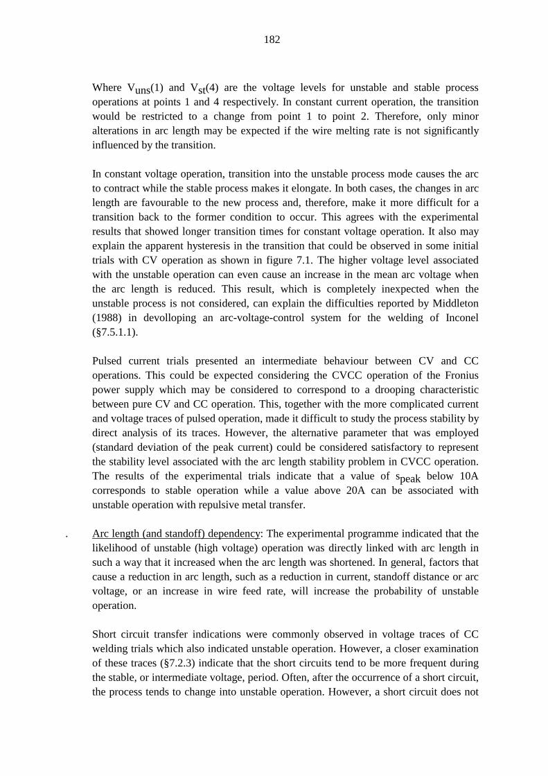
182
Where Vuns(1) and Vst(4) are the voltage levels for unstable and stable processoperations at points 1 and 4 respectively. In constant current operation, the transitionwould be restricted to a change from point 1 to point 2. Therefore, only minoralterations in arc length may be expected if the wire melting rate is not significantlyinfluenced by the transition.
In constant voltage operation, transition into the unstable process mode causes the arcto contract while the stable process makes it elongate. In both cases, the changes in arclength are favourable to the new process and, therefore, make it more difficult for atransition back to the former condition to occur. This agrees with the experimentalresults that showed longer transition times for constant voltage operation. It also mayexplain the apparent hysteresis in the transition that could be observed in some initialtrials with CV operation as shown in figure 7.1. The higher voltage level associatedwith the unstable operation can even cause an increase in the mean arc voltage whenthe arc length is reduced. This result, which is completely inexpected when theunstable process is not considered, can explain the difficulties reported by Middleton(1988) in devolloping an arc-voltage-control system for the welding of Inconel(§7.5.1.1).
Pulsed current trials presented an intermediate behaviour between CV and CCoperations. This could be expected considering the CVCC operation of the Froniuspower supply which may be considered to correspond to a drooping characteristicbetween pure CV and CC operation. This, together with the more complicated currentand voltage traces of pulsed operation, made it difficult to study the process stability bydirect analysis of its traces. However, the alternative parameter that was employed(standard deviation of the peak current) could be considered satisfactory to representthe stability level associated with the arc length stability problem in CVCC operation.The results of the experimental trials indicate that a value of speak below 10Acorresponds to stable operation while a value above 20A can be associated withunstable operation with repulsive metal transfer.
. Arc length (and standoff) dependency: The experimental programme indicated that thelikelihood of unstable (high voltage) operation was directly linked with arc length insuch a way that it increased when the arc length was shortened. In general, factors thatcause a reduction in arc length, such as a reduction in current, standoff distance or arcvoltage, or an increase in wire feed rate, will increase the probability of unstableoperation.
Short circuit transfer indications were commonly observed in voltage traces of CCwelding trials which also indicated unstable operation. However, a closer examinationof these traces (§7.2.3) indicate that the short circuits tend to be more frequent duringthe stable, or intermediate voltage, period. Often, after the occurrence of a short circuit,the process tends to change into unstable operation. However, a short circuit does not
183
seems to be essential for transition from Vst to Vuns which frequently takes placespontaneously.
In CC operation, both Vst and Vuns increase with the standoff distance and, in mostcases, the relationship between these parameters and the standoff distance is reasonablyrepresented by straight lines (figures 7.23 and 7.24 and table 7.9). On the other hand,the difference between Vuns and Vst seems to be less sensitive to the standoffdistance.
. Influence of shielding gas composition: Only two gas additions (helium and oxygen) toa base gas (argon) were studied in the present programme. Oxygen was considered thekey factor in controlling the arc length dependent instability problem while helium wasinvestigated because of its potential in terms of improving fusion in GMAW.
In all the shielding mixtures that contained argon which were evaluated, oxygenadditions tended to reduce the likelihood of the unstable process. No significant effectcould be detected in a few constant current trials made with He and He-O2 mixtures. InCV trials, additions of oxygen resulted in shorter tus and lower minimum voltagevalues to prevent initial instability (table 7.8). Although no arc length measurementswere performed, visual observation of the arc indicated that, when oxygen was present,stable operation could be achieved at shorter arc lengths.
In CC trials, the relative frequency of Vuns periods at any standoff distance was muchlower for Ar-2%O2 than pure Ar. For all standoff distances over 14mm, the Vunsperiods were reduced to sharp spikes when using Ar-2%O2. Oxygen additions causedan overall reduction in the voltage level for stable operation (Vst), although the Vunscurve seemed to be essentially unaffected. The mean voltage tended also to be lower inAr-2%O2 due to the reductions in both Vus and unstable operation frequency. Theslope of the Vst to standoff relationship for Ar-2%O2 welding is also significantlylower than the slope for welding in pure Ar (table 7.9 and figure 7.37). Assuming thatthe electrode stickout is approximately independent of the standoff distance forconstant current operation, the slope of the Vst to standoff curve can be used to obtaina rough estimate of the arc electric field strength, E. The value obtained in the presentprogramme for pure argon shielding (640 ± 120 V/m), although close to, can beconsidered smaller, with a 95% significance level, than the value commonly presentedin the literature (800 V/m). For Ar-2%O2 shielding, an even smaller value (310 ± 40V/m) was found.
Both CC and pulsed current experimental trials indicate that a helium content up toapproximately 75% does not significantly affect arc behaviour with regard to the arclength process instability problem. Oxygen additions to mixtures containing up to thislevel of helium are effective in terms of reducing arc instability/metal transferproblems. In pure helium shielding, metal transfer tended to be globular, independentof the arc length, for the current levels used. As the spray-globular transition current
184
for helium shielding is considered higher than for argon (Rimskii et al. 1979), it ispossible that, at current levels greater than those used here, spray transfer may beobserved with helium shielding. In the CC tests, pure He shielded welding wasapparently less unstable at longer standoff distances. This can be observed in thefrequency plots of figures 7.17 and 7.22, by the narrower voltage distribution forlonger standoff. As the standoff distance decreases, the stability of the helium shieldedtrials worsens considerably, abundant short circuiting happens and the mean processvoltage drops sharply to levels that are even below the mean voltage for Ar-75%Hewelding. The difference between Vuns and Vst was shown to decrease at a rate ofapproximately 5E-2 V/%He with the helium content in the shielding gas (figure 7.25).This reduction is associated with the tendency of Vst to increase faster than Vuns withthe content of He in the shielding (figures 7.23 and 7.24). The slope of both Vst andVuns against the standoff distance also increase with the helium content (figure 7.37and table 7.9).
. Effect of welding current: The results of CC trials indicated that an increase in thewelding current from 260A to 300A causes the difference between Vuns and Vst todrop by approximately 1.5V independent of the helium content in the mixture (figure7.25).
. Effect of joint type: Although no systematic study was performed to evaluate theinfluence of the joint type on the process stability, some results of pulsed current trialsseem to suggest that narrow gap welding presents a lower sensitivity to instabilitywhen compared with bead-on-plate welding (figure 7.27).
7.5.1.3.Tentative mechanism
The present experimental work revealed a clear association between arc length dependentinstability problems and oxygen levels in the shielding gas. The favourable influence ofoxygen in both arc stability, metal transfer and bead shape in GMAW welding of steel is wellestablished. In terms of arc stability, oxide films are considered essential to the formation andstabilization of cathode spots which are generally located on the workpiece and close to themolten pool (Essers and van Gospel 1984, §2.2.2). When welding with pure argon shieldingis performed on a relatively clean steel plate, the arc will quickly consume the oxide layerbeside the weld pool and move outwards erratically on the surface of the plate resulting in aprocess that is more difficult to control (Boughton and Amin 1972). In the presence of anoxidising medium, the oxide layer located close to weld pool can be continuouslyregenerated resulting in the arc root being fixed at this position.
Experimental results elsewhere indicate that the addition of up to 5% oxygen to argon canreduce the spray-globular transition current of steel consumables. This reduction has beenrelated to different factors such as increase in arc temperature (Brosilow 1978), magneticeffects associated with the paramagnetic nature of oxygen (Rimskii et all. 1979) and a
185
reduction in the surface tension of the molten electrode tip (Kennedy 1970, Norrish andHilton 1988).
Finally, the presence of an oxidising component in the shielding can smooth the weld beadprofile, reducing its wetting angle and reinforcement height, improve bead penetration andreduce undercutting tendency by decreasing the surface tension of the molten pool (Salterand Dye 1971, Norrish and Hilton 1988) or stabilizing the position of the arc root (Cresswell1972).
It is the view of the author of the present work that it has demonstrated the existence of afurther aspect of arc rooting problems that is closely related to arc length and the oxidisingpotential of the shielding gas. This particular phenomenon, although closely related torelatively well established aspects of the gas shielded welding of steel and resulting in strongchanges in process behaviour, does not seem to have been reported in the literature to date.Instabilities at the start of GMA welds on steel are commonly observed and often explainedby experienced welders by the low initial temperature of the workpiece. When working witha CV power supply, the arc tends to revert into stable operation a few seconds after itsinitiation, hence the problem has not been perceived as significant. In constant currentoperation, however, the transition in operating mode do not necessarily result in a longer arcand, if the shielding gas has a low oxidising potential (2% or less of oxygen or carbondioxide), the instable period can last longer, particularly, if a short arc is being used.
Although the experimental work in the present programme has not been planned to explorethe fine details of arc physics that would be necessary for a more complete understanding ofthis arc length dependent instability, a tentative descriptive model can be developed toexplain some aspects of the phenomenon.
Figure 7.38 presents a schematic representation of the GMAW arc region. Point C indicatesthe location of the cathode spots and the displacement r corresponds to their position inrelation to the electrode-arc axis (OA). Under a shielding gas relatively rich in oxygen, thecathode spots will be located just at the edge of the weld pool and r will be at its minimumvalue. However, if the oxidising potential of the shielding gas is not sufficiently high, thecathodic region may have to expand in order to reach fresh oxide areas and r will be greaterthan this minimum value. An estimate of r can be obtained by considering that the oxide areathat should be consumed by the arc per unit time in order to sustain the welding current (AI)results both from fresh oxide areas that are brought to the arc region by welding torchtranslation (Av) and surface oxide created in the arc region by any oxygen presented in theshielding (AO):
AI = Av + AO [7.14]
In a first approximation, AO can be considered proportional to the partial pressure of oxygen(pO2) in the shielding:
186
AO = k0.pO2 [7.15]
and:
Av = (2r).v [7.16]
where v is the welding speed. Therefore, by rearranging equations [7.14], [7.15] and [7.16]:
vpkAr OI
220−
= [7.17]
Boughton and Amin Mian (1972) estimate that a 0.2 to 0.5 µm thick oxide layer would beconsumed by the arc at a rate of 0.6 mm2/As. So, for a 250A arc, AI _ 150 mm2/s. If theshielding gas is pure argon (pO2=0) and the welding speed is 7mm/s, the calculateddisplacement r of the cathodic region would be equal to approximately 10mm. In thepresence of a small amount of oxygen in the shielding gas, r would be quickly reduced to itsminimum value.
The cathodic displacement will result in an increase in the real arc length of the process. Anestimate of this length can be given by (figure 7.38):
la(r) = (r2 + la2)1/2 [7.18]
Which forms an angle _ with the electrode-arc axis:
θ = tan-1(r/la) [7.19]
Both la(r) and θ will increase if r increases, for instance, by decreasing the oxygen potentialin the shielding. θ can also be increased by decreasing the arc length la. For very short arcoperation, θ can become so large that it would be very difficult for the arc to preserve itscontact with the cathodic region and the resulting system would be very unstable. In thiscondition the arc may either extinguish or change to a different operating condition. It isproposed here that the latter can take place by the development of a new cathode spotoperating under a different mechanism and located on the weld pool surface. Differentmechanisms have been proposed in the literature for cold cathode operation, althoughmainly, in relation to vacuum arc processes. Vapour dominated cathodes are reported todevelop in vacuum arcs on oxide free surfaces (Guile 1982) and their presence has also beensuggested in welding arcs (Bougthon and Amin Mian 1972). Changes in cathode operationmechanisms in vacuum arcs have been associated with abrupt variation in voltage (Fu 1989).
Based on the aspects discussed above, a descriptive model can be proposed for the arc lengthinstability process (figure 7.39). For a given welding condition, r is approximately constant ifthe process is operating only in "stable" mode and is given by equation [7.17]. In this case, ifthe arc is shortened for any reason, θ will tend to increase and the existence of a critical value
187
of θ (θc), can then be postulated above which maintenance of contact with the cathodicregion (point c, figure 7.39(a)) is so difficult that a new cathode spot (point c', figure 7.39(b))is formed at the centre of the weld pool. This new cathode spot would operate by amechanism possibly independent from surface contamination which, by being lessenergetically favourable than the previous condition, would result in a higher arc voltage(figure 7.39(c)). As the cathodic region would now be concentrated only one spot, a plasmajet directed from the weld pool to the electrode would be formed and would tend to blow themolten tip of the wire away from the pool, i. e., metal transfer would change into a repulsivemode. During single spot operation, oxide layers on the surface of the workpiece would notbe consumed and would be brought closer to the arc region by both translation of the torchand surface reoxidation. Consequently, for a fixed arc length θ would decrease and make iteasier for the process to operate again from the oxide sites, cathode spots would be formedback on the plate surface, the arc shape would change and spray operation would be restoredfor a period of time during which the oxide layer would be consumed. θ would increase againcreating conditions for the formation of a new single spot in the pool.
Therefore, the welding system would tend to alternate periods of multi- and single-spotoperation with different voltage levels as observed in the CC operation trials (figure 7.39(c)).In a shielding gas containing oxygen, r would tend to be smaller than in pure inert gaswelding (equation [7.17]). Consequently, a smaller value of la(r) could be expected whichwould partially explain the lower Vst values of welding trials with Ar-2%O2 compared withpure argon. Lower values of r and θ would also reduce the tendency to unstable periods. InCV welding, the transition from stable to unstable mode will shorten the arc as discussed in§7.5.1.2 causing a further increase in _ that would make it even more difficult for the processto return to stable operation. Similar but opposite changes in la and θ would apply to thetransition from unstable to stable operation.
The descriptive model presented above is obviously an oversimplification of the complexprocesses taking place in the arc during the changes in operation stability. Even so, itprovides reasonable explanations for many aspects of the phenomenon such as arc length andoxygen dependencies and the influence of the power supply. The model does not consider theinfluence of time and, therefore, cannot deal with the apparent greater likelihood of unstableoperation in the first moments of welding. Time dependency may be linked somehow withworkpiece temperature distribution but no explanation was found for it.
7.5.2.Shielding gas/process optimization
7.5.2.1.Shielding gas
According to different authors additions of helium to an argon based shielding gas result inseveral changes in arc shape and behaviour, metal transfer and weld bead characteristics(§2.2.5). Generally, the results obtained in the present programme seem to agree well with
188
previous works regarding the influence of the helium content in shielding on the weldingcharacteristics.
It has been found that fusion characteristics in both bead-on-plate and narrow gap weldingwas improved by increasing %He in the shielding. This improvement in fusion was mainlyassociated with an increase in secondary fusion in the workpiece whereas fusion related tofinger penetration was little affected. Gurev and Stout (1963) related plate fusion in GMAWwith two distinct mechanisms: (a)the finger-shaped region would be formed by the action ofarc pressure and superheated metal drops on the workpiece and (b)the approximatelyelliptical region out of the finger (secondary fusion region) that would be formed with timeby heat transport in the weld pool from the arc and the finger region. Regarding the fingerpenetration, the present results seem to indicate that the net arc action on the plate was littleaffected by gas composition under the pulsed welding conditions employed. The secondaryfusion was, however, positively influenced by the higher energy of the arc associated with thepresence of helium which resulted in a higher arc voltage (figure 7.40).
An unfavourable influence of helium content was found above 75% He when metal transferand arc stability deteriorate, probably due to a sharp increase in the spray-globular transitioncurrent. Furthermore, oxygen additions appear to reduce problems of arc length dependentinstability for all the gas compositions studied except pure helium.
Based on these results it was decided to implement in experimental steps S2-B1 and S3-B1(chapter 5) a gas mixture containing approximately 75%He, 2%O2 and argon. This gascomposition was considered to achieve a balance between good arc stability and improvedfusion in the ternary system Ar-He-O2.
7.5.2.2.Power supply characteristics
The analysis of the interactions between power supply characteristics and joint geometryperformed in section §7.4 indicated that, in a narrow gap joint two extremes situations cantake place:
(a) For a short arc operation (here "short" means an arc shorter than approximately half ofthe gap width) the process resembles bead-on-plate operation as far as its interactionswith the power supply are concerned. Therefore, in short arc operation some arc self-adjustment capability based on a constant voltage component in the power supplycharacteristic will be desirable to control and prevent wire stubbing on the plate.
(b) For long arc operation, however, such a constant voltage component would result inthe process presenting unstable behaviour in terms of arc length control.
In an attempt to optimize the power supply response to the gap geometry and based onequipment available a mixed characteristic operation was implemented in experimental steps

189
S2-B1 and S3-B1 (chapter 5). This proposed operational mode involved constant voltagecharacteristic below a certain limit and constant current above this limit (figure 7.41). Thisoperation with mixed characteristics allows control of arc length for short arc operation anddoes not generate a tendency for unstable arc wander along the joint side walls.
7.5.2.3.Steady and pulsed current
Based on the results of previous work (Fennel 1986), experimental blocks S0 and S1 (chapter5) were performed with pulsed CVCC operation. However, once the mean welding currentwas generally kept above the spray-globular transition for a 1.2mm wire, the use of simplercontinuous current operation could be considered. Even though it was considered thatprocess stability might be impaired by the move into steady current, it was expected that theuse of a current close to the transition level together with the optimized gas mixture wouldprevent a major worsening in process stability. Furthermore, steady current operation couldresult in a substantial reduction in wire melting rate by reducing the Joule heating of the wire.This reduction can be estimated through equation [2.13b]:
w - wnp = βs(Ip - Ib)2tptb/(tp + tb) [2.13b]
Taking ß = 5x10⁻⁵ A-2s-1 (Allum 1983), and supposing, for instance, s = 18mm, Ip= 500A,Ib= 100A, tp= 2ms and tb= 3ms as typical values for pulsed operation, the calculatedincrease in melting rate in pulsed current operation due to Joule effect would over 2m/min.As low dilution and, consequently, fusion defects were major problems associated with theprocess, the reduction in fusion was considered to have a potential beneficial effect in termsof reducing fusion problems and was, therefore, adopted in experimental steps S2 and S3.
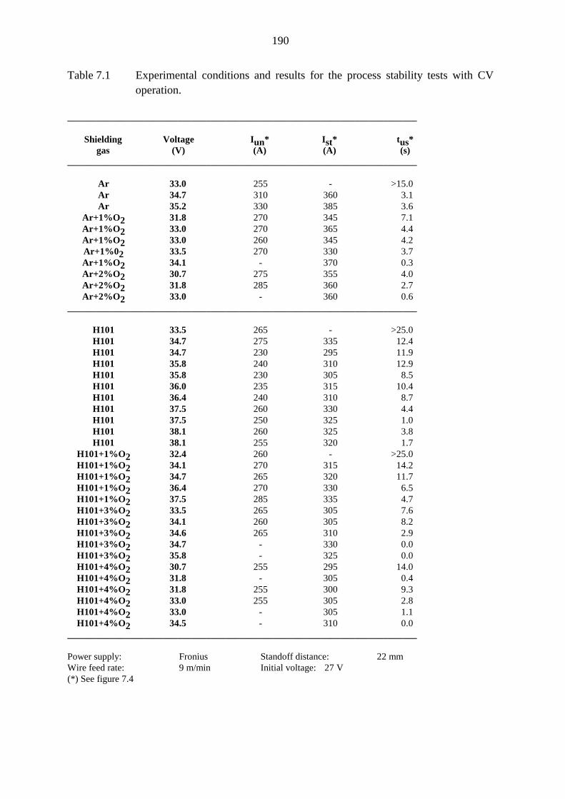
190
Table 7.1 Experimental conditions and results for the process stability tests with CVoperation.
_________________________________________________________________________
Shielding Voltage Iun* Ist* tus*gas (V) (A) (A) (s)
_________________________________________________________________________
Ar 33.0 255 - >15.0Ar 34.7 310 360 3.1Ar 35.2 330 385 3.6
Ar+1%O2 31.8 270 345 7.1Ar+1%O2 33.0 270 365 4.4Ar+1%O2 33.0 260 345 4.2Ar+1%02 33.5 270 330 3.7Ar+1%O2 34.1 - 370 0.3Ar+2%O2 30.7 275 355 4.0Ar+2%O2 31.8 285 360 2.7Ar+2%O2 33.0 - 360 0.6
_________________________________________________________________________
H101 33.5 265 - >25.0H101 34.7 275 335 12.4H101 34.7 230 295 11.9H101 35.8 240 310 12.9H101 35.8 230 305 8.5H101 36.0 235 315 10.4H101 36.4 240 310 8.7H101 37.5 260 330 4.4H101 37.5 250 325 1.0H101 38.1 260 325 3.8H101 38.1 255 320 1.7
H101+1%O2 32.4 260 - >25.0H101+1%O2 34.1 270 315 14.2H101+1%O2 34.7 265 320 11.7H101+1%O2 36.4 270 330 6.5H101+1%O2 37.5 285 335 4.7H101+3%O2 33.5 265 305 7.6H101+3%O2 34.1 260 305 8.2H101+3%O2 34.6 265 310 2.9H101+3%O2 34.7 - 330 0.0H101+3%O2 35.8 - 325 0.0H101+4%O2 30.7 255 295 14.0H101+4%O2 31.8 - 305 0.4H101+4%O2 31.8 255 300 9.3H101+4%O2 33.0 255 305 2.8H101+4%O2 33.0 - 305 1.1H101+4%O2 34.5 - 310 0.0
_________________________________________________________________________
Power supply: Fronius Standoff distance: 22 mmWire feed rate: 9 m/min Initial voltage: 27 V(*) See figure 7.4

191
Table 7.2 Experimental conditions used with the constant current process stabilitytrials.
______________________________________________________________________
Trial Shielding Welding Wire Standoff# gas current feed rate distance OBS
(A) (m/min) (mm)______________________________________________________________________
A1 Ar 260 8 14A2 Ar 260 8 17A3 Ar 260 8 17A4 Ar 260 8 20A5 Ar 260 8 20A6 Ar 260 8 20A7 Ar 260 8 23A8 Ar 260 8 23A9 Ar 260 8 26
A10 Ar 260 8 26 ChamberA11 Ar 260 8 29 ChamberA12 Ar 260 8 32 Chamber
______________________________________________________________________
A13 Ar 300 10 14A14 Ar 300 10 17A15 Ar 300 10 17A16 Ar 300 10 20A17 Ar 300 10 20A18 Ar 300 10 23
______________________________________________________________________
B1 Ar-25%He 260 8 14B2 Ar-25%He 260 8 17B3 Ar-25%He 260 8 20B4 Ar-25%He 260 8 23
______________________________________________________________________
B5 Ar-25%He 260 10 14B6 Ar-25%He 260 10 20B7 Ar-25%He 260 10 23B8 Ar-25%He 260 10 26
______________________________________________________________________
B9 Ar-25%He 300 10 14B10 Ar-25%He 300 10 17B11 Ar-25%He 300 10 20B12 Ar-25%He 300 10 23
______________________________________________________________________cont.
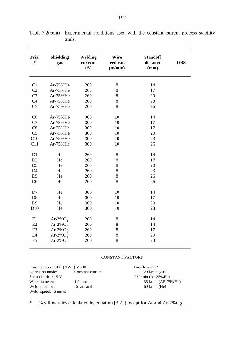
192
Table 7.2(cont) Experimental conditions used with the constant current process stabilitytrials.
_________________________________________________________________
Trial Shielding Welding Wire Standoff# gas current feed rate distance OBS
(A) (m/min) (mm)_________________________________________________________________
C1 Ar-75%He 260 8 14C2 Ar-75%He 260 8 17C3 Ar-75%He 260 8 20C4 Ar-75%He 260 8 23C5 Ar-75%He 260 8 26
C6 Ar-75%He 300 10 14C7 Ar-75%He 300 10 17C8 Ar-75%He 300 10 17C9 Ar-75%He 300 10 20
C10 Ar-75%He 300 10 23C11 Ar-75%He 300 10 26
D1 He 260 8 14D2 He 260 8 17D3 He 260 8 20D4 He 260 8 23D5 He 260 8 26D6 He 260 8 26
D7 He 300 10 14D8 He 300 10 17D9 He 300 10 20
D10 He 300 10 23
E1 Ar-2%O2 260 8 14E2 Ar-2%O2 260 8 14E3 Ar-2%O2 260 8 17E4 Ar-2%O2 260 8 20E5 Ar-2%O2 260 8 23
_________________________________________________________________
CONSTANT FACTORS
Power supply: GEC (AWP) M500 Gas flow rate*:Operation mode: Constant current 20 l/min (Ar)Short cir. det.: 15 V 23 l/min (Ar-25%He)Wire diameter: 1.2 mm 35 l/min (AR-75%He)Weld. position: Downhand 60 l/min (He)Weld. speed: 6 mm/s
* Gas flow rates calculated by equation [3.2] (except for Ar and Ar-2%O2).
193
Table 7.3 Results of the constant current process stability trials.
_________________________________________________________________
Trial Standoff Vmean Vst Vuns# distance (V) (V) (V)
(mm)_________________________________________________________________
A1 14 28.6 25.5 34.0A2 17 30.6 27.0 36.5A3 17 29.8 26.5 36.0A4 20 30.9 28.3 37.5A5 20 31.0 28.5 37.0A6 20 29.2 28.5 38.0A7 23 31.9 31.9 -A8 23 31.4 31.4 -A9 26 32.0 32.0 -A10 26 34.8 31.4 40.0A11 29 35.4 34.2 41.9A12 32 37.4 37.4 -A13 14 28.6 25.8 33.3A14 17 31.9 28.3 34.3A15 17 31.9 27.3 34.0A16 20 32.0 32.0 -A17 20 32.2 30.0 36.5A18 23 34.5 34.5 -B1 14 31.0 27.5 35.3B2 17 32.9 28.8 36.8B3 20 34.0 32.0 38.0B4 23 35.7 36.0 -B5 14 25.3 25.0 31.5B6 20 30.9 28.0 35.0B7 23 33.5 29.8 36.0B8 26 36.7 30.8 38.0B9 14 30.9 28.8 34.5B10 17 32.5 30.5 35.0B11 20 36.0 36.0 -B12 23 37.0 37.0 -
_________________________________________________________________
cont.
194
Table 7.3(cont) Results of the constant current process stability trials.
_________________________________________________________________
Trial Standoff Vmean Vst Vuns# distance (V) (V) (V)
(mm)_________________________________________________________________
C1 14 32.2 30.0 36.0C2 17 36.6 33.0 39.0C3 20 38.6 36.0 41.0C4 23 40.3 39.5 42.8C5 26 42.0 42.0 -C6 14 32.5 31.5 35.3C7 17 37.4 36.0 38.5C8 17 37.2 35.5 38.5C9 20 40.2 38.0 41.5C10 23 42.2 41.0 44.3C11 26 43.7 43.7 -D1 14 30.8 - -D2 17 33.6 - -D3 20 41.4 - -D4 23 43.9 - -D5 26 45.0 - -D6 26 44.6 - -D7 14 32.4 - -D8 17 34.9 - -D9 20 41.9 - -D10 23 43.3 - -E1 14 26.7 23.5 36.0E2 14 25.7 23.5 36.0E3 17 24.5 24.5 37.5E4 20 25.5 25.5 39.0E5 23 26.2 26.2 -
_________________________________________________________________
195
Table 7.4 Experimental conditions and measured current structure parameters in thepulsed current trials with He-1 and He-2 gases.
_____________________________________________________________________Gas Wire feed Imean Ipeak speak tpeak Frequency
rate(m/min) (A) (A) (A) (ms) (Hz)_____________________________________________________________________
He1 10 274 454 57 2.11 199He1 12 307 513 35 2.31 200
_____________________________________________________________________He1+3%O2 10 267 449 7 2.07 200He1+3%O2 10 270 453 8 2.09 200He1+3%O2 11 270 452 48 2.06 203He1+3%O2 11 270 460 53 2.10 200He1+3%O2 12 287 482 43 2.23 200_____________________________________________________________________He1+5%O2 10 269 447 7 2.10 200He1+5%O2 11 274 463 6 2.14 200He1+5%O2 11 279 468 7 2.16 200He1+5%O2 12 286 483 14 2.23 200He1+5%O2 12 287 485 18 2.24 199_____________________________________________________________________
He2 10 252 480 45 2.14 198He2 11 269 499 34 2.26 197He2 12 277 504 32 2.35 197He2 12 310 512 37 2.31 196
_____________________________________________________________________He2+3%O2 10 248 480 9 2.14 190He2+3%O2 11 249 481 55 2.12 190_____________________________________________________________________He2+5%O2 10 246 473 5 2.17 191He2+5%O2 11 257 497 9 2.19 191He2+5%O2 12 265 502 15 2.26 192_____________________________________________________________________
196
Table 7.5 Experimental conditions for bead-on-plate and narrow gap welding trialswith different Ar-He-2%O2 shielding mixtures.
__________________________________________________Trial Ar/He Specimen Ib
# ratio type* (A)__________________________________________________1 1/0 BP 502 1/0 BP 503 1/0 NG 504 1/0 NG 50
____________________________________________________5 7/3 BP 506 7/3 BP 507 7/3 NG 508 7/3 NG 50__________________________________________________9 3/7 BP 10010 3/7 BP 10011 3/7 BP 10012 3/7 NG 10013 3/7 NG 100__________________________________________________
14 0/1 BP 10015 0/1 BP 10016 0/1 NG 10017 0/1 NG 100__________________________________________________
CONSTANT FACTORS
Power supply: Fronius TPS500 Peak voltage: 40 VOperation mode: CVCC pulsed Peak time: 2 msGas flow rate: see table 4.9 Frequency: 200 HzWire diameter: 1.2 mm Weld. position: DownhandGap width: 7 mm Weld. speed: 7 mm/sWire feed rate: 12 m/min___________________________________________________________________________________* BP - Bead-on-plate welding NG - Narrow gap welding
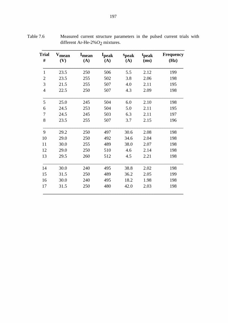
197
Table 7.6 Measured current structure parameters in the pulsed current trials withdifferent Ar-He-2%O2 mixtures.
______________________________________________________________Trial Vmean Imean Ipeak speak tpeak Frequency
# (V) (A) (A) (A) (ms) (Hz)_____________________________________________________________1 23.5 250 506 5.5 2.12 1992 23.5 255 502 3.8 2.06 1983 21.5 255 507 4.0 2.11 1954 22.5 250 507 4.3 2.09 198_____________________________________________________________5 25.0 245 504 6.0 2.10 1986 24.5 253 504 5.0 2.11 1957 24.5 245 503 6.3 2.11 1978 23.5 255 507 3.7 2.15 196_____________________________________________________________9 29.2 250 497 30.6 2.08 19810 29.0 250 492 34.6 2.04 19811 30.0 255 489 38.0 2.07 19812 29.0 250 510 4.6 2.14 19813 29.5 260 512 4.5 2.21 198_____________________________________________________________14 30.0 240 495 38.8 2.02 19815 31.5 250 489 36.2 2.05 19916 30.0 240 495 18.2 1.98 19817 31.5 250 480 42.0 2.03 198_____________________________________________________________
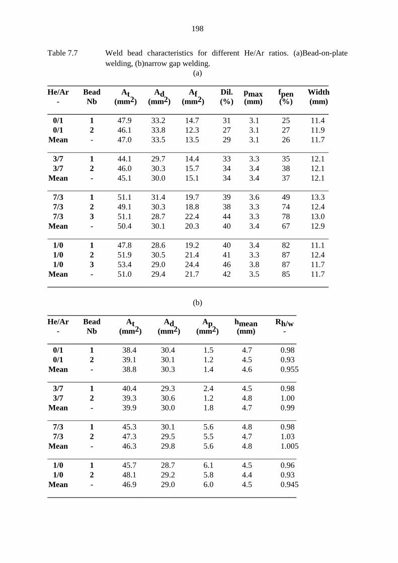
198
Table 7.7 Weld bead characteristics for different He/Ar ratios. (a)Bead-on-platewelding, (b)narrow gap welding.
(a)______________________________________________________________________He/Ar Bead At Ad Af Dil. pmax fpen Width
- Nb (mm2) (mm2) (mm2) (%) (mm) (%) (mm)______________________________________________________________________
0/1 1 47.9 33.2 14.7 31 3.1 25 11.40/1 2 46.1 33.8 12.3 27 3.1 27 11.9
Mean - 47.0 33.5 13.5 29 3.1 26 11.7______________________________________________________________________
3/7 1 44.1 29.7 14.4 33 3.3 35 12.13/7 2 46.0 30.3 15.7 34 3.4 38 12.1
Mean - 45.1 30.0 15.1 34 3.4 37 12.1______________________________________________________________________
7/3 1 51.1 31.4 19.7 39 3.6 49 13.37/3 2 49.1 30.3 18.8 38 3.3 74 12.47/3 3 51.1 28.7 22.4 44 3.3 78 13.0
Mean - 50.4 30.1 20.3 40 3.4 67 12.9______________________________________________________________________
1/0 1 47.8 28.6 19.2 40 3.4 82 11.11/0 2 51.9 30.5 21.4 41 3.3 87 12.41/0 3 53.4 29.0 24.4 46 3.8 87 11.7
Mean - 51.0 29.4 21.7 42 3.5 85 11.7______________________________________________________________________
(b)______________________________________________________________He/Ar Bead At Ad Ap hmean Rh/w
- Nb (mm2) (mm2) (mm2) (mm) -______________________________________________________________
0/1 1 38.4 30.4 1.5 4.7 0.980/1 2 39.1 30.1 1.2 4.5 0.93
Mean - 38.8 30.3 1.4 4.6 0.955______________________________________________________________
3/7 1 40.4 29.3 2.4 4.5 0.983/7 2 39.3 30.6 1.2 4.8 1.00
Mean - 39.9 30.0 1.8 4.7 0.99______________________________________________________________
7/3 1 45.3 30.1 5.6 4.8 0.987/3 2 47.3 29.5 5.5 4.7 1.03
Mean - 46.3 29.8 5.6 4.8 1.005______________________________________________________________
1/0 1 45.7 28.7 6.1 4.5 0.961/0 2 48.1 29.2 5.8 4.4 0.93
Mean - 46.9 29.0 6.0 4.5 0.945______________________________________________________________
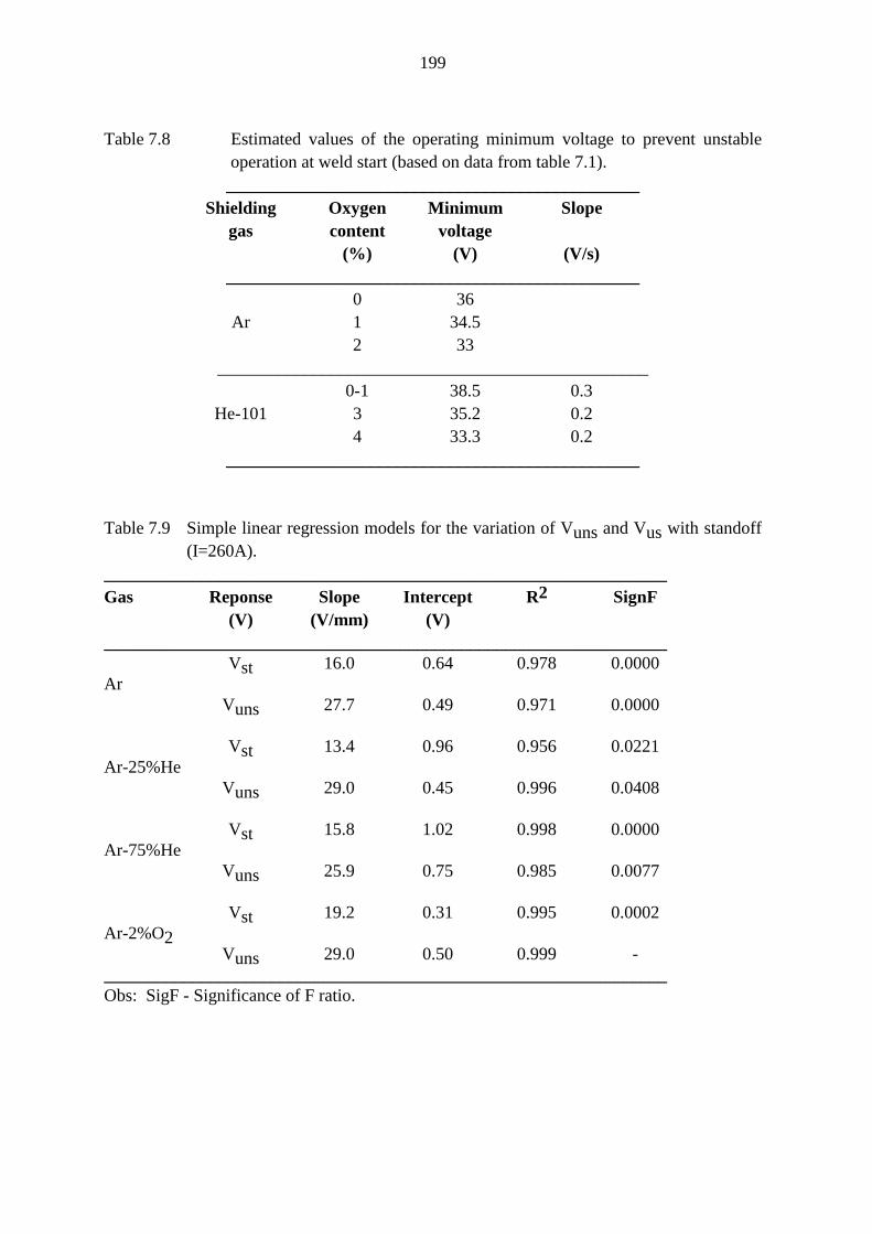
199
Table 7.8 Estimated values of the operating minimum voltage to prevent unstableoperation at weld start (based on data from table 7.1).
_______________________________________________Shielding Oxygen Minimum Slope
gas content voltage(%) (V) (V/s)
_______________________________________________0 36
Ar 1 34.52 33
_________________________________________________0-1 38.5 0.3
He-101 3 35.2 0.24 33.3 0.2
_______________________________________________
Table 7.9 Simple linear regression models for the variation of Vuns and Vus with standoff(I=260A).
________________________________________________________________Gas Reponse Slope Intercept R2 SignF
(V) (V/mm) (V)________________________________________________________________
Vst 16.0 0.64 0.978 0.0000Ar
Vuns 27.7 0.49 0.971 0.0000
Vst 13.4 0.96 0.956 0.0221Ar-25%He
Vuns 29.0 0.45 0.996 0.0408
Vst 15.8 1.02 0.998 0.0000Ar-75%He
Vuns 25.9 0.75 0.985 0.0077
Vst 19.2 0.31 0.995 0.0002Ar-2%O2
Vuns 29.0 0.50 0.999 -________________________________________________________________Obs: SigF - Significance of F ratio.
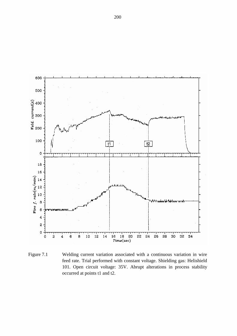
200
Figure 7.1 Welding current variation associated with a continuous variation in wirefeed rate. Trial performed with constant voltage. Shielding gas: Helishield101. Open circuit voltage: 35V. Abrupt alterations in process stabilityoccurred at points t1 and t2.
201
Figure 7.2 Schematic representation of the stable (a) and unstable (b) operationalmodes.
Figure 7.3 Sloped welding specimen.
202
Figure 7.4 Constant voltage stability test result. Iun - current level at unstable mode,Ist - current level at stable mode, and tus time necessary for the change totake place from unstable to stable mode.
203
Figure 7.5 Effect of oxygen content and voltage on the time necessary for processstabilization.
204
(a)
(b)
Figure 7.6 Schematic drawing from the IMACON photographs of the arc for the CVstability trials. (a)Spray transfer, (b)repulsive drop transfer.
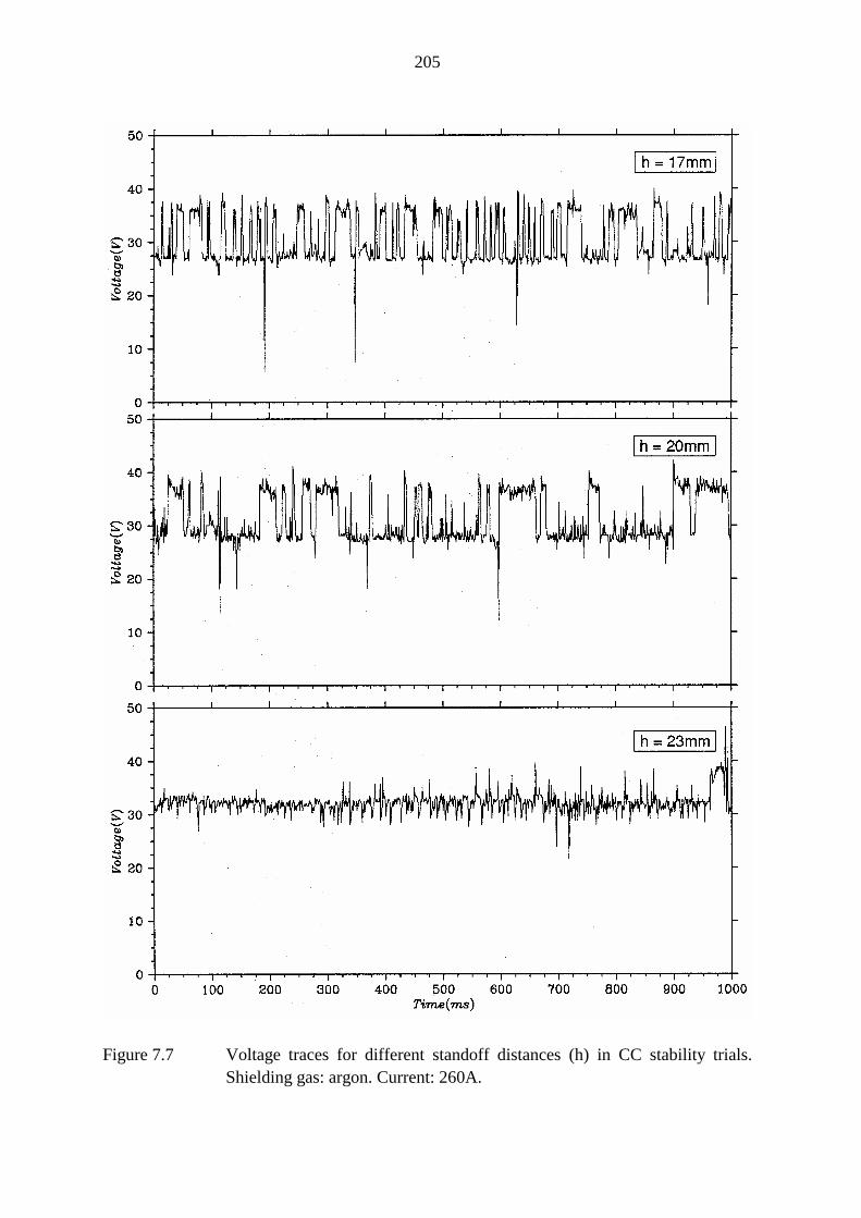
205
Figure 7.7 Voltage traces for different standoff distances (h) in CC stability trials.Shielding gas: argon. Current: 260A.
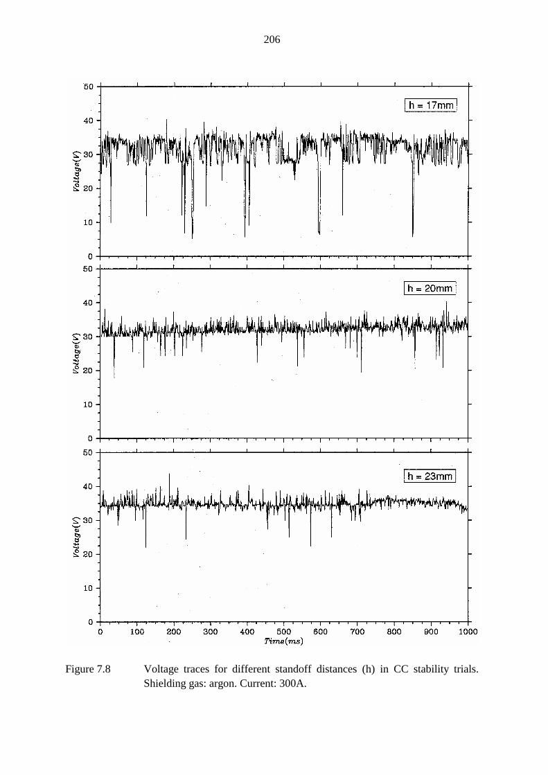
206
Figure 7.8 Voltage traces for different standoff distances (h) in CC stability trials.Shielding gas: argon. Current: 300A.
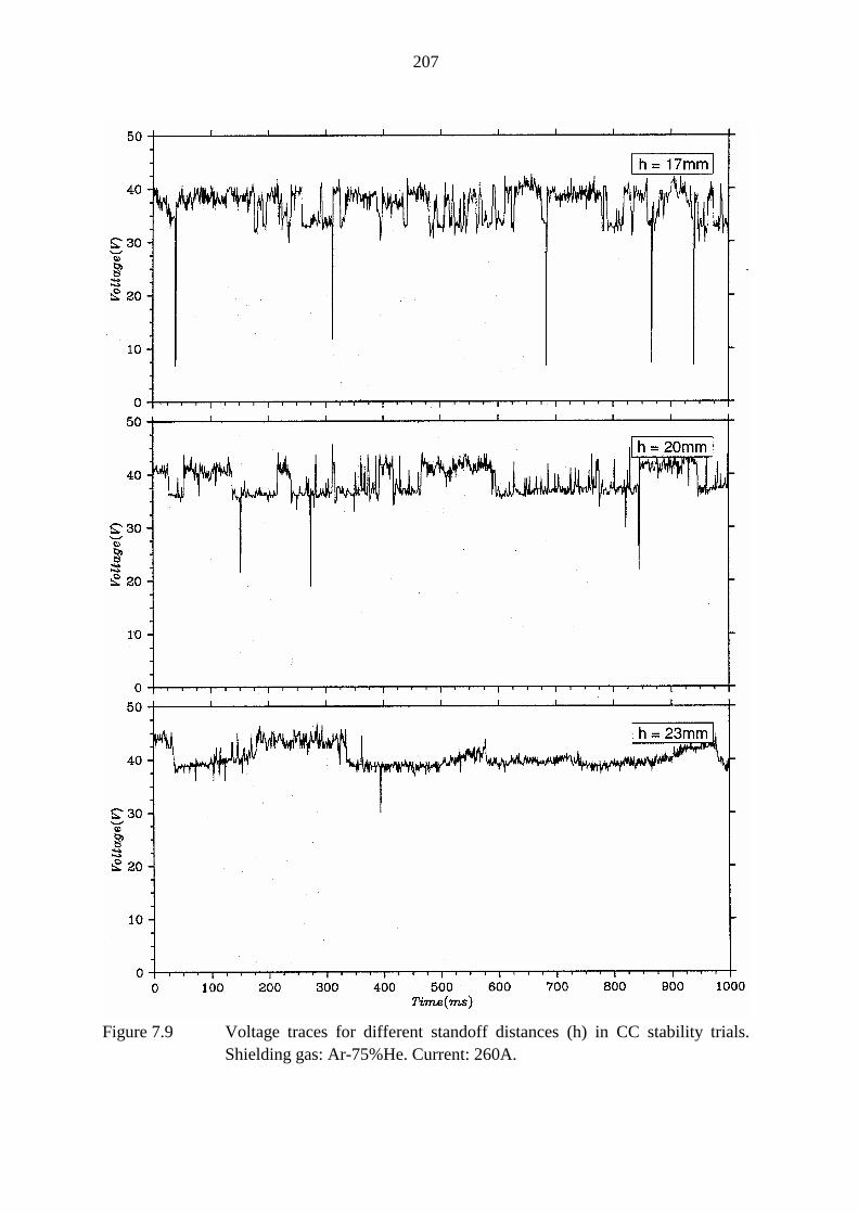
207
Figure 7.9 Voltage traces for different standoff distances (h) in CC stability trials.Shielding gas: Ar-75%He. Current: 260A.
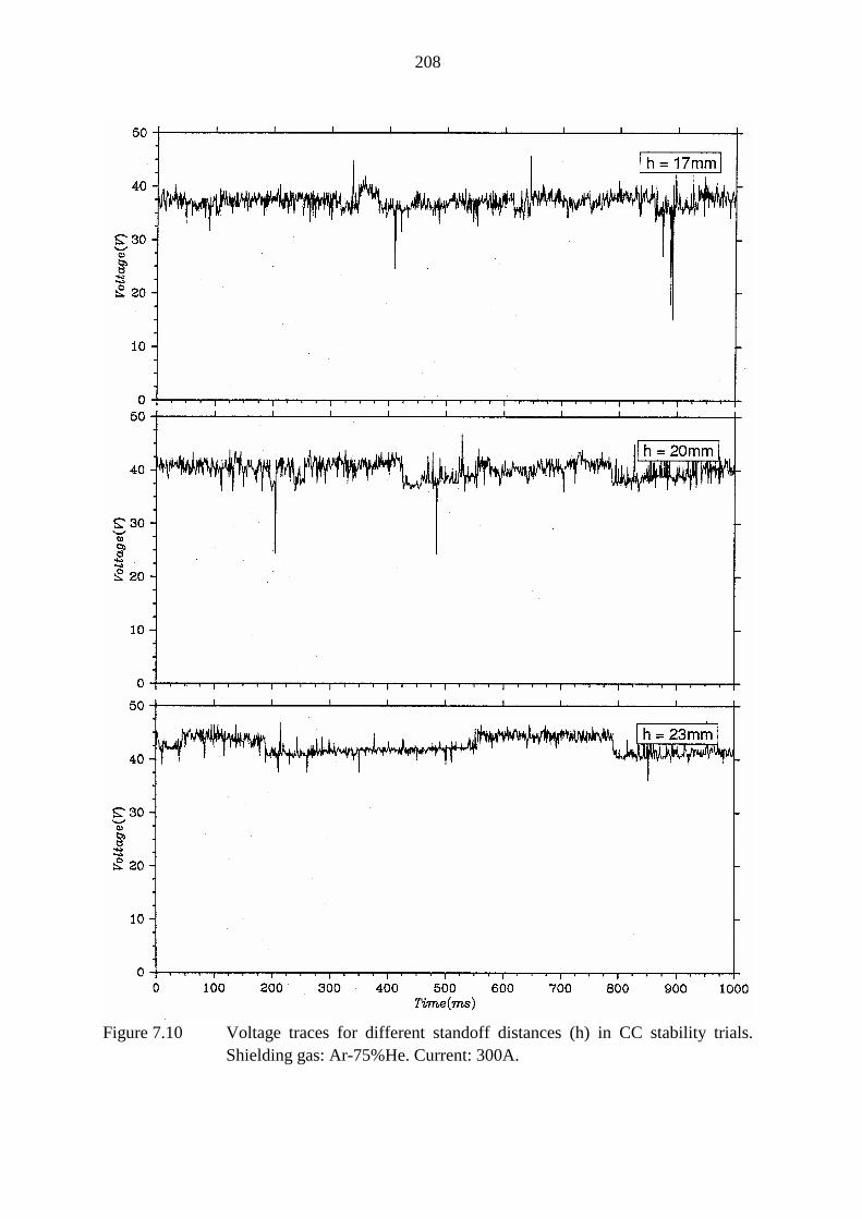
208
Figure 7.10 Voltage traces for different standoff distances (h) in CC stability trials.Shielding gas: Ar-75%He. Current: 300A.
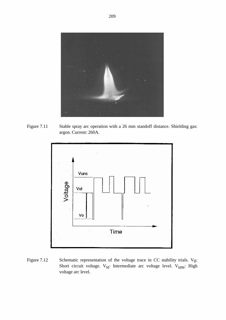
209
Figure 7.11 Stable spray arc operation with a 26 mm standoff distance. Shielding gas:argon. Current: 260A.
Figure 7.12 Schematic representation of the voltage trace in CC stability trials. V0:Short circuit voltage. Vst: Intermediate arc voltage level. Vuns: Highvoltage arc level.
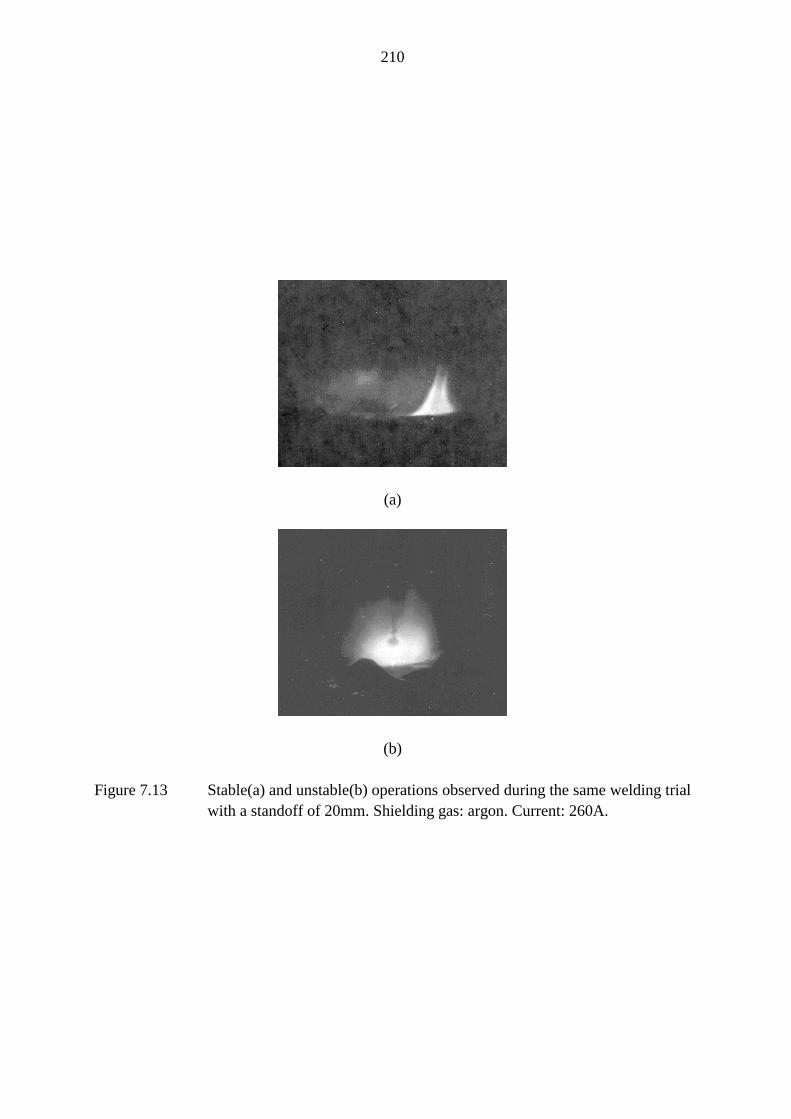
210
(a)
(b)
Figure 7.13 Stable(a) and unstable(b) operations observed during the same welding trialwith a standoff of 20mm. Shielding gas: argon. Current: 260A.
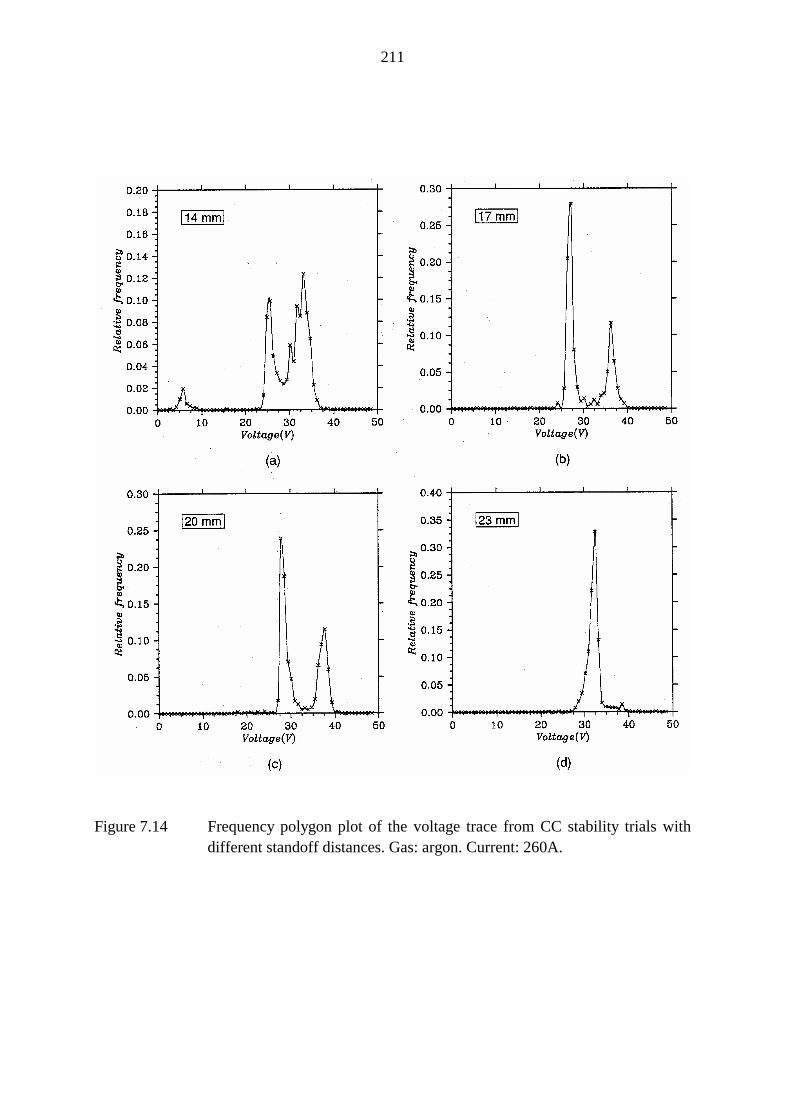
211
Figure 7.14 Frequency polygon plot of the voltage trace from CC stability trials withdifferent standoff distances. Gas: argon. Current: 260A.
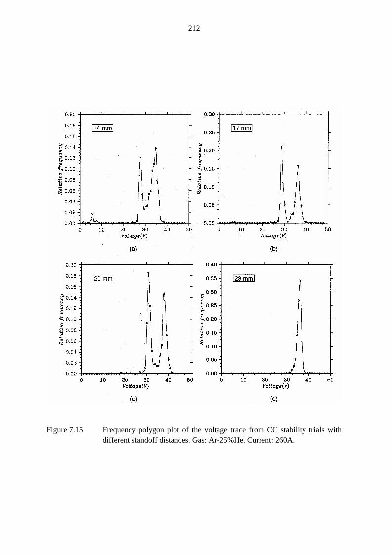
212
Figure 7.15 Frequency polygon plot of the voltage trace from CC stability trials withdifferent standoff distances. Gas: Ar-25%He. Current: 260A.
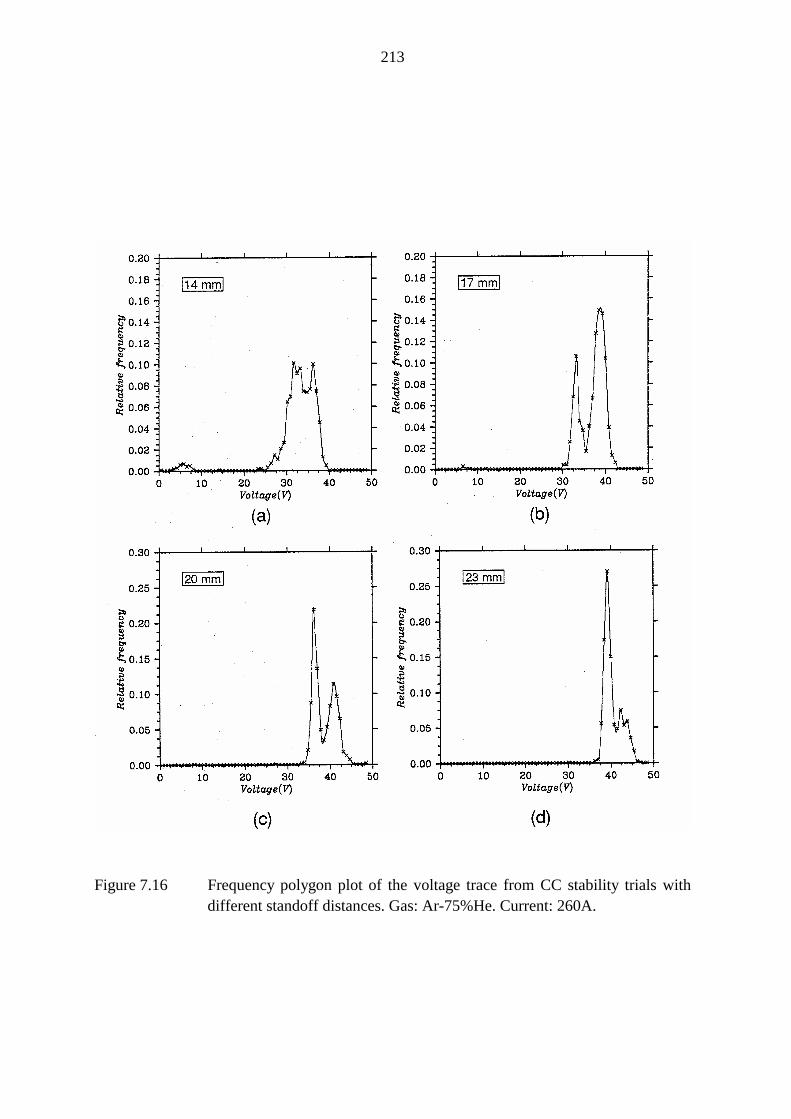
213
Figure 7.16 Frequency polygon plot of the voltage trace from CC stability trials withdifferent standoff distances. Gas: Ar-75%He. Current: 260A.
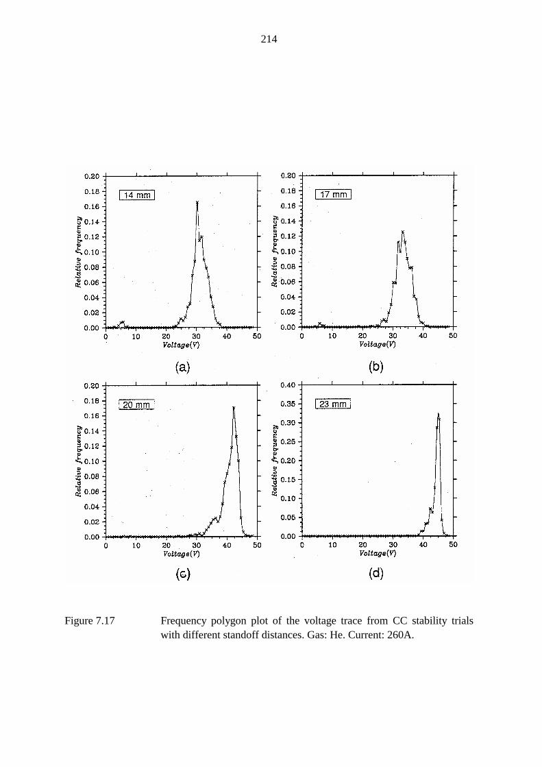
214
Figure 7.17 Frequency polygon plot of the voltage trace from CC stability trialswith different standoff distances. Gas: He. Current: 260A.
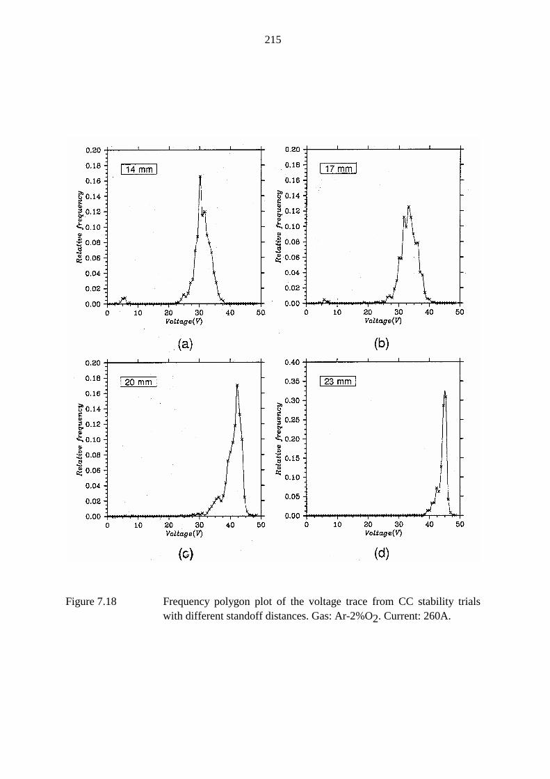
215
Figure 7.18 Frequency polygon plot of the voltage trace from CC stability trialswith different standoff distances. Gas: Ar-2%O2. Current: 260A.
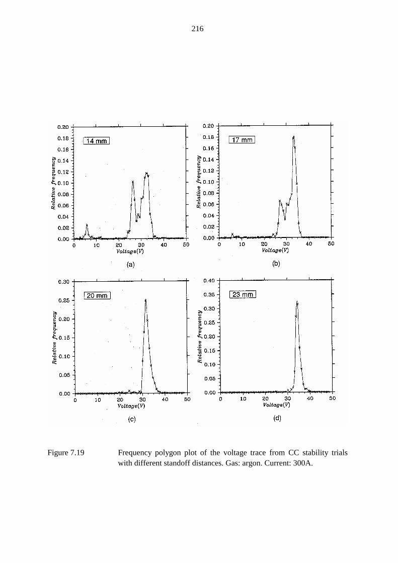
216
Figure 7.19 Frequency polygon plot of the voltage trace from CC stability trialswith different standoff distances. Gas: argon. Current: 300A.
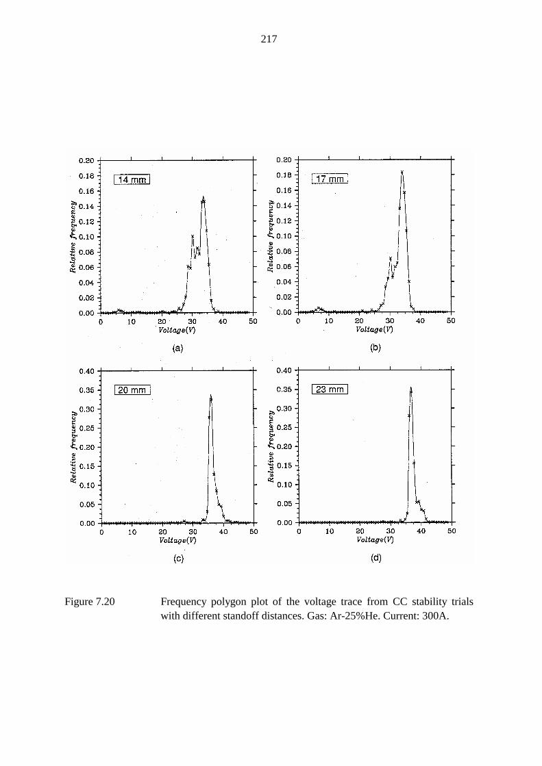
217
Figure 7.20 Frequency polygon plot of the voltage trace from CC stability trialswith different standoff distances. Gas: Ar-25%He. Current: 300A.
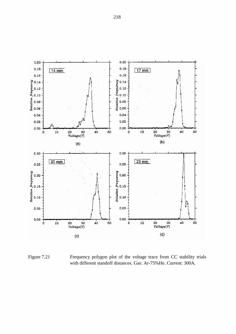
218
Figure 7.21 Frequency polygon plot of the voltage trace from CC stability trialswith different standoff distances. Gas: Ar-75%He. Current: 300A.
219
Figure 7.22 Frequency polygon plot of the voltage trace from CC stability trialswith different standoff distances. Gas: He. Current: 300A.
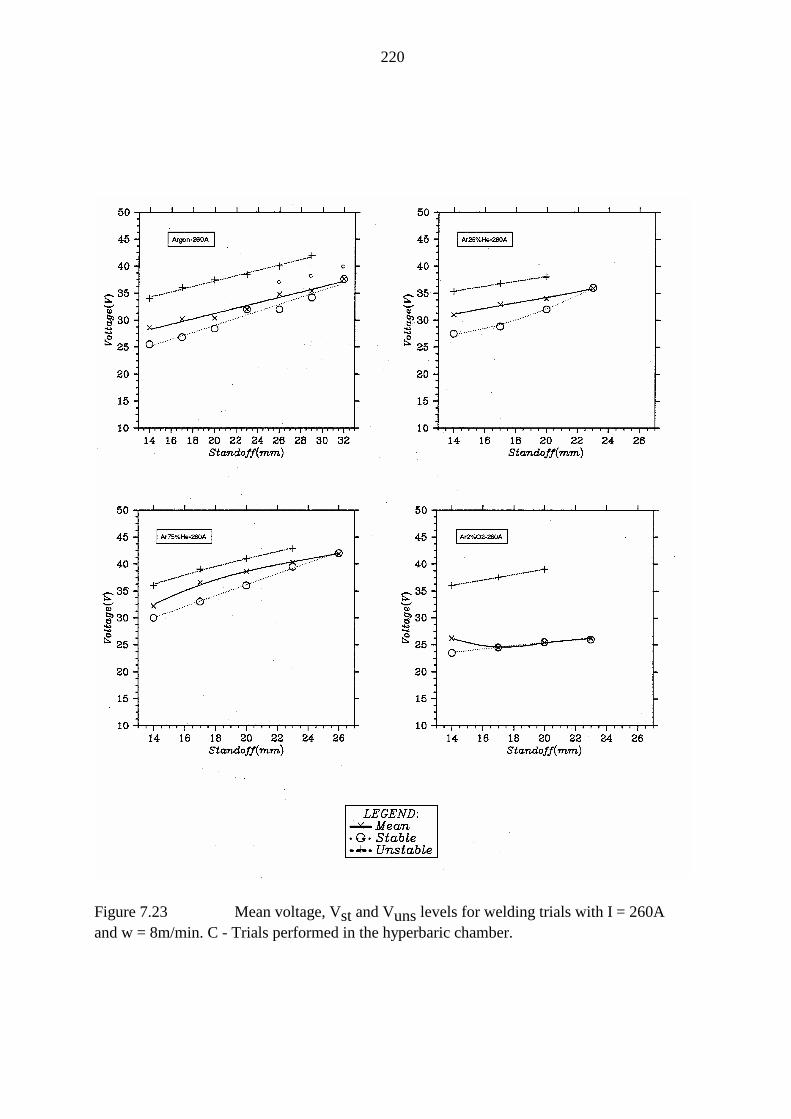
220
Figure 7.23 Mean voltage, Vst and Vuns levels for welding trials with I = 260Aand w = 8m/min. C - Trials performed in the hyperbaric chamber.
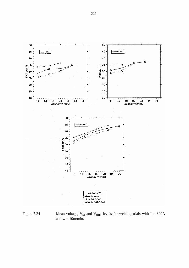
221
Figure 7.24 Mean voltage, Vst and Vuns levels for welding trials with I = 300Aand w = 10m/min.
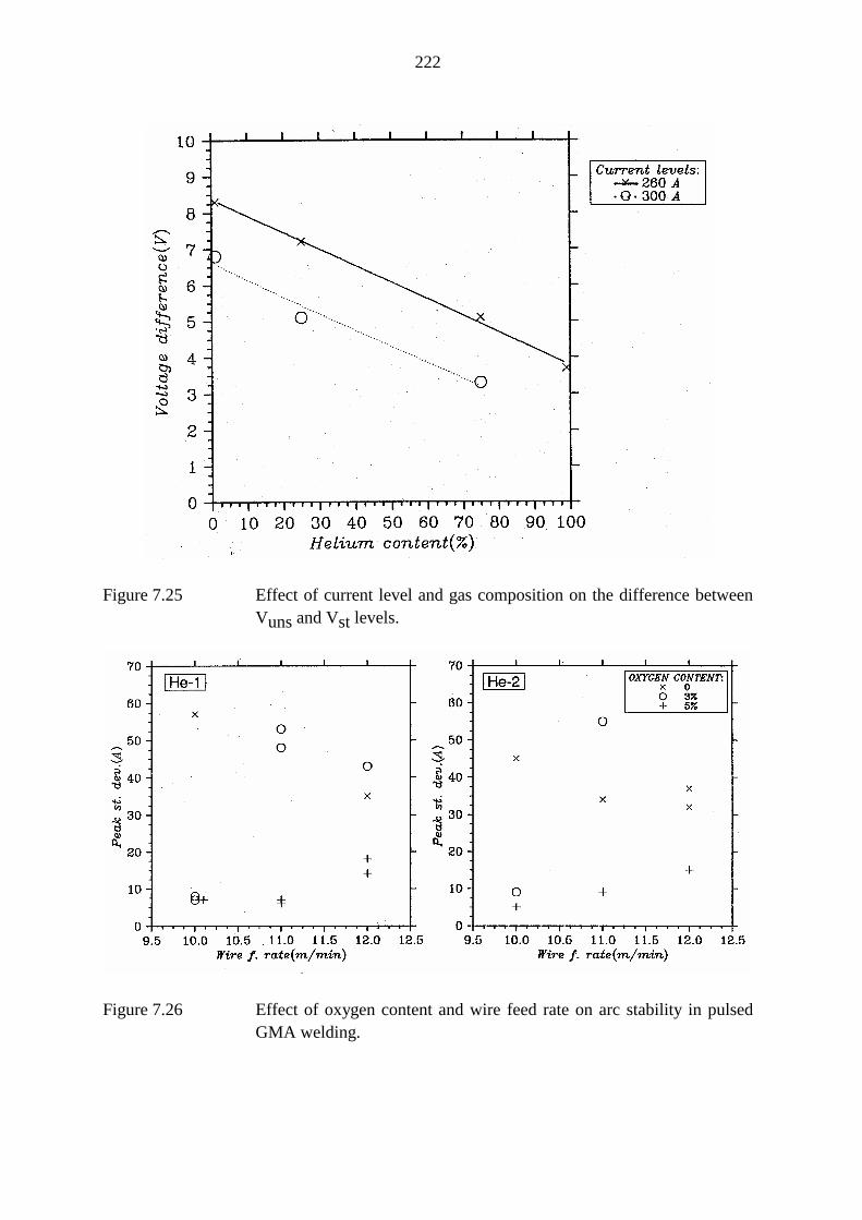
222
Figure 7.25 Effect of current level and gas composition on the difference betweenVuns and Vst levels.
Figure 7.26 Effect of oxygen content and wire feed rate on arc stability in pulsedGMA welding.
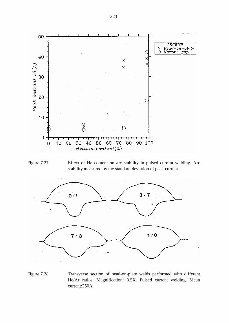
223
Figure 7.27 Effect of He content on arc stability in pulsed current welding. Arcstability measured by the standard deviation of peak current.
Figure 7.28 Transverse section of bead-on-plate welds performed with differentHe/Ar ratios. Magnification: 3.5X. Pulsed current welding. Meancurrent:250A.
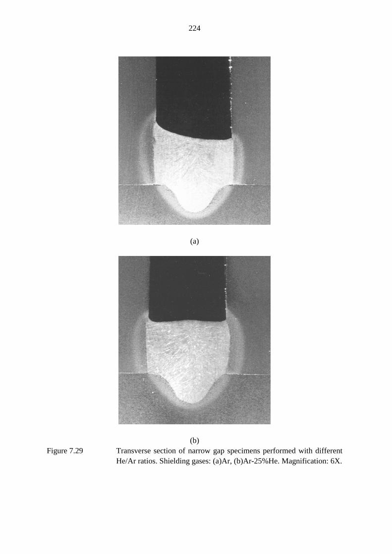
224
(a)
(b)Figure 7.29 Transverse section of narrow gap specimens performed with different
He/Ar ratios. Shielding gases: (a)Ar, (b)Ar-25%He. Magnification: 6X.
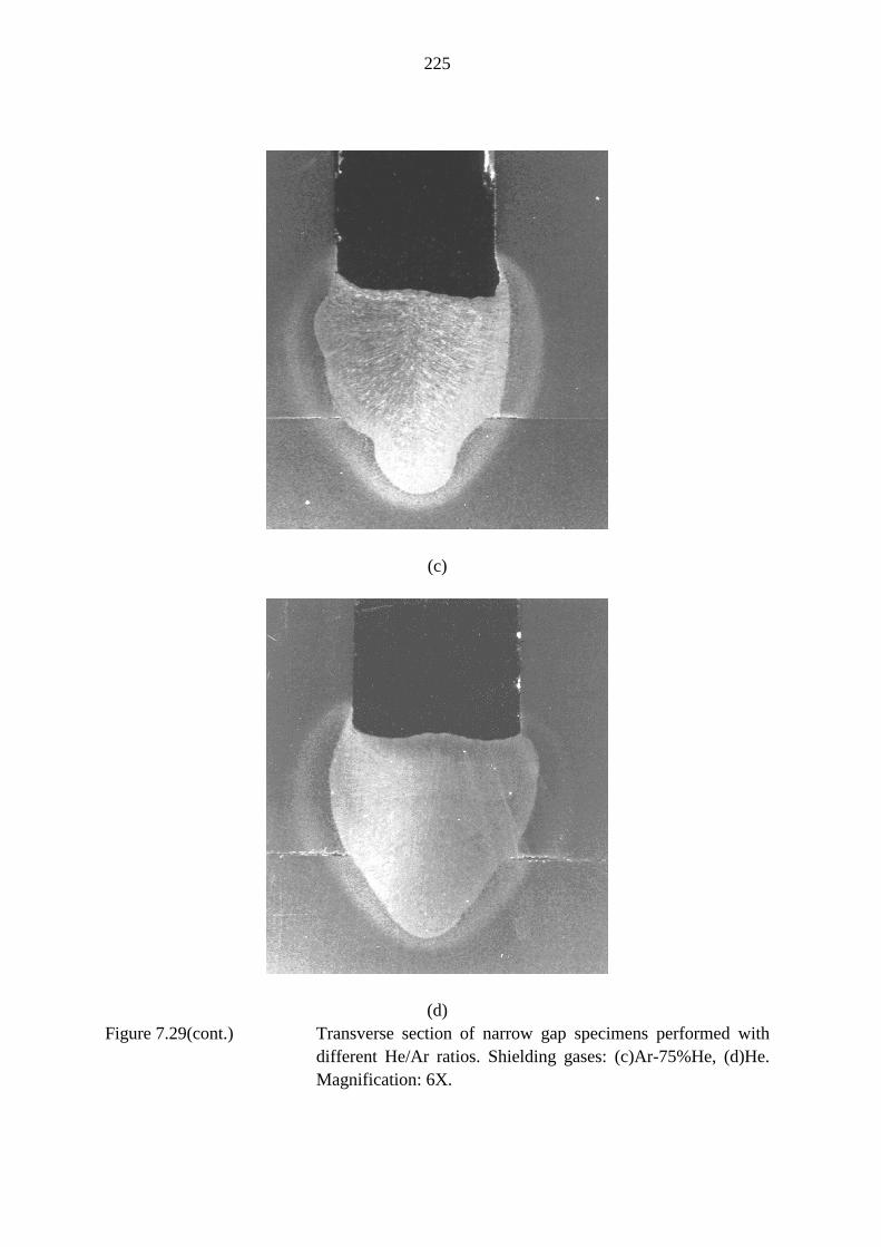
225
(c)
(d)Figure 7.29(cont.) Transverse section of narrow gap specimens performed with
different He/Ar ratios. Shielding gases: (c)Ar-75%He, (d)He.Magnification: 6X.
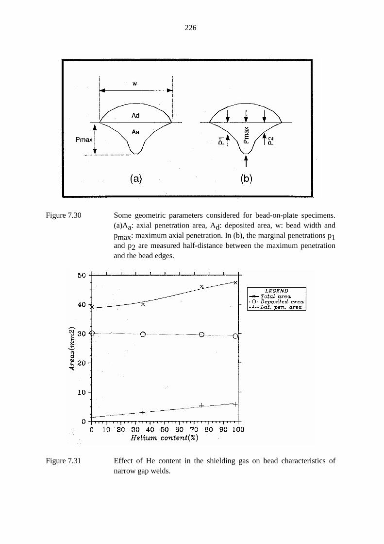
226
Figure 7.30 Some geometric parameters considered for bead-on-plate specimens.(a)Aa: axial penetration area, Ad: deposited area, w: bead width andpmax: maximum axial penetration. In (b), the marginal penetrations p1and p2 are measured half-distance between the maximum penetrationand the bead edges.
Figure 7.31 Effect of He content in the shielding gas on bead characteristics ofnarrow gap welds.
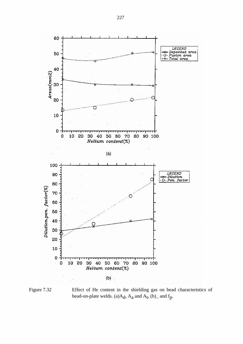
227
Figure 7.32 Effect of He content in the shielding gas on bead characteristics ofbead-on-plate welds. (a)Ad, Aa and At, (b)_ and fp.
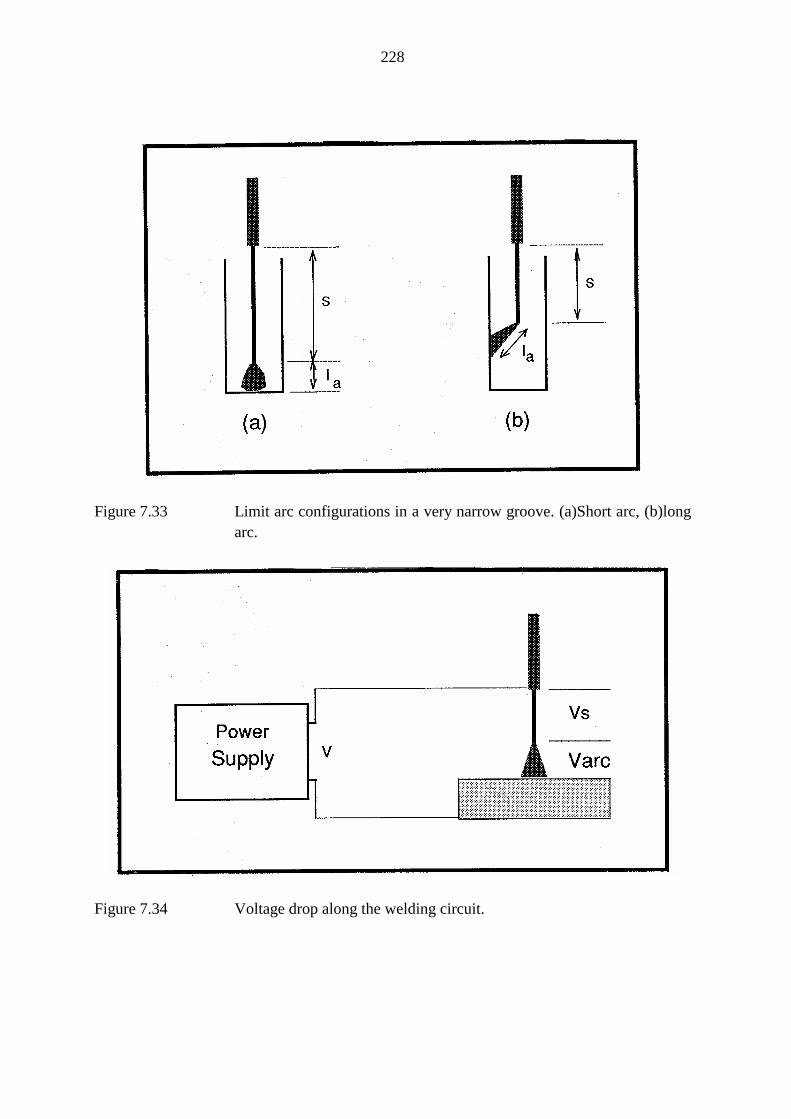
228
Figure 7.33 Limit arc configurations in a very narrow groove. (a)Short arc, (b)longarc.
Figure 7.34 Voltage drop along the welding circuit.
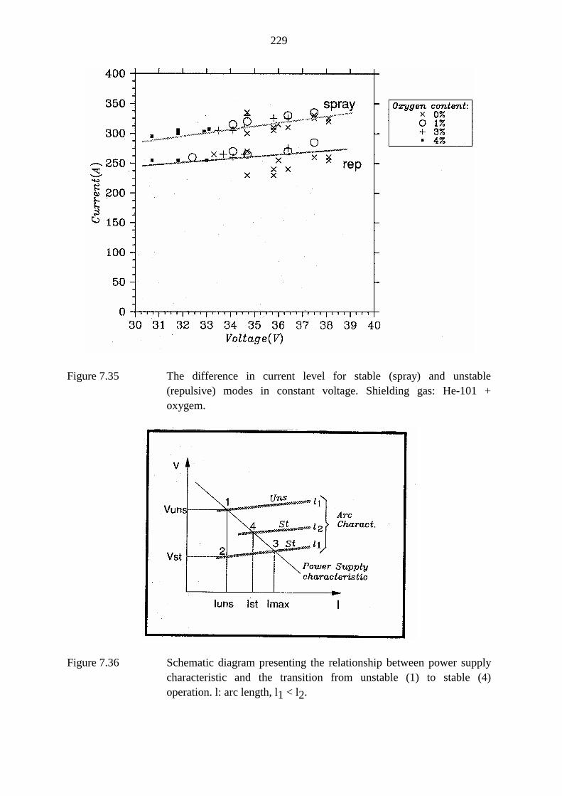
229
Figure 7.35 The difference in current level for stable (spray) and unstable(repulsive) modes in constant voltage. Shielding gas: He-101 +oxygem.
Figure 7.36 Schematic diagram presenting the relationship between power supplycharacteristic and the transition from unstable (1) to stable (4)operation. l: arc length, l1 < l2.
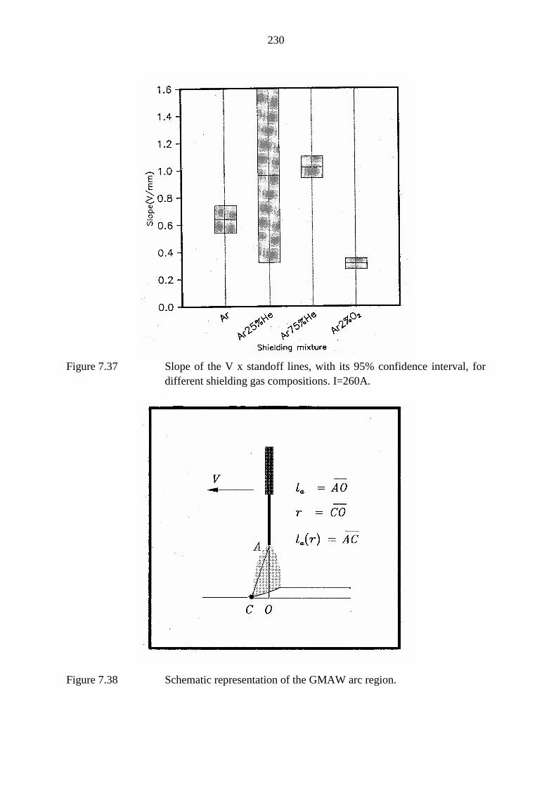
230
Figure 7.37 Slope of the V x standoff lines, with its 95% confidence interval, fordifferent shielding gas compositions. I=260A.
Figure 7.38 Schematic representation of the GMAW arc region.
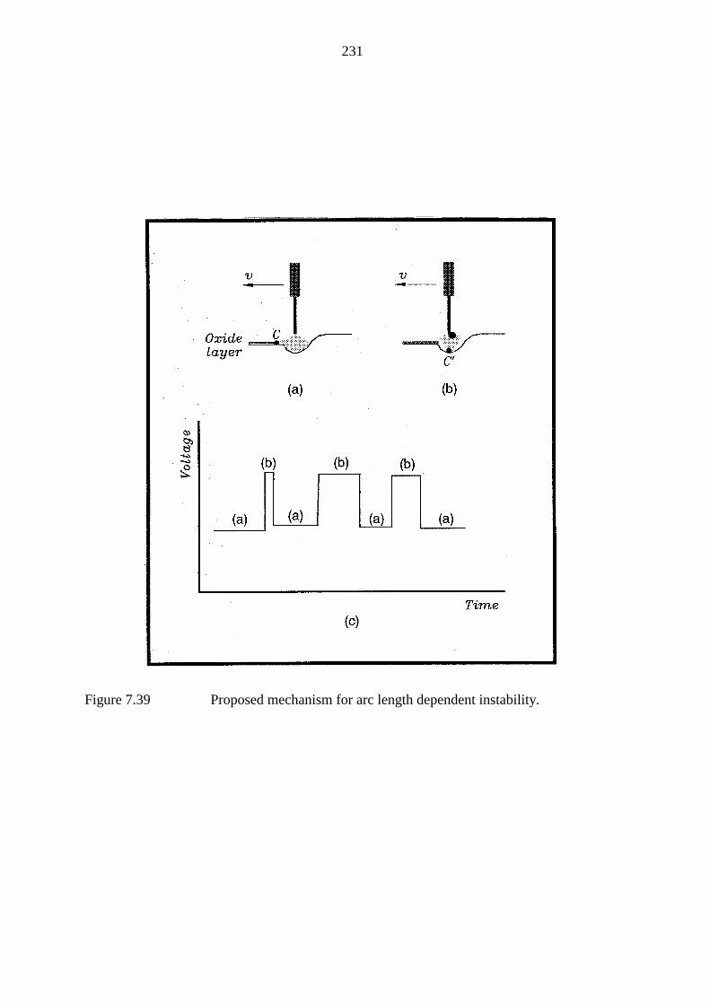
231
Figure 7.39 Proposed mechanism for arc length dependent instability.
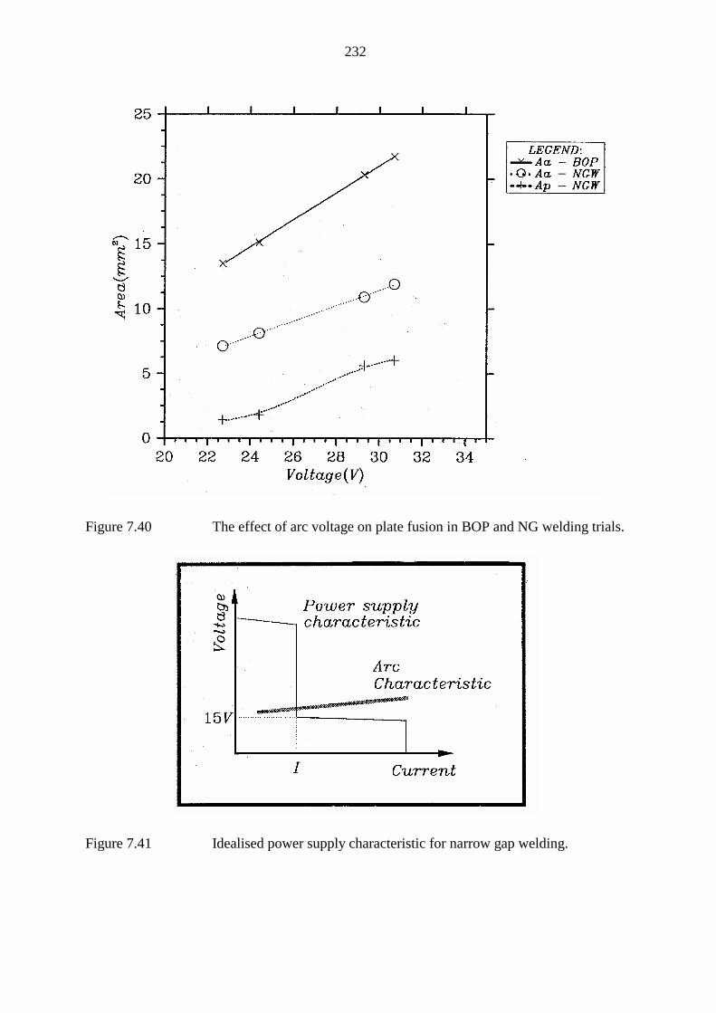
232
Figure 7.40 The effect of arc voltage on plate fusion in BOP and NG welding trials.
Figure 7.41 Idealised power supply characteristic for narrow gap welding.

CHAPTER 8
234
8. CONCLUSIONS
1. Statistical experimental analysis can provide a powerful tool for the analysis andmodelling of welding processes. The present programme demonstrated that thesetechniques can be a more efficient and adequate tool than the usual one-variable-at-a-time approach to investigate the influence of welding parameters on the weld beadcharacteristics. However, caution is important to avoid misleading conclusions froman improper use of these techniques. The strong interdependence between inputvariables that was found in the GMAW-NG process made it difficult to apply afactorial experiment in its analysis. This forced the use of a distorted factorial whichintroduced some collinearity into the input data. Careful data analysis, however,allowed the development of adequate models by multiple linear regression.
2. Modelling results depend strongly on both the experimental design and the initialset of input variable candidates, and this should be taken into account during resultanalysis. For example, modelling equations for bead characteristics related to wirefusion can be reduced to a very simple form by properly selecting input variables.The objectives of modelling and the experimental conditions should influence thisselection.
3. Plate melting efficiency decreases in NGW with decreasing gap width and is alwayslower than in bead-on-plate welding. The chance of sidewall fusion defects at thebottom of the joint generally decreases with decreasing gap width.
4. For the downhand position, the best results in terms of a lack of welding defectswere associated with non-pulsed, constant current operation, Ar-He-O2 shieldingand a 7mm gap width. The optimized shielding gas mixture and the use of a non-pulsed current enlarged considerably the space for acceptable operation of theprocess. This improvement was demonstrated by a multiplot diagram in which theinfluence of four different input variables could be analyzed at the same time. Inhorizontal-vertical welding, the main process feature was non-uniform plate fusionby the arc. In order to minimize this effect by forcing a more effective arc action,measures such as narrower gap widths or off-centre wire positioning should beused.
5. Helium additions to the shielding gas improve both lateral and axial penetration inNGW. The increase in plate fusion is related to an increase in secondary fusionwhile finger penetration remains approximately unchanged. Results indicate that upto 75%He can be used in the shielding gas without process stability deterioratingappreciably in NGW provided an adequate balance of oxidizing components ispresent.

235
6. Helium additions to the shielding gas can enlarge the area of acceptable operation inNG-GMA welding by improving its fusion characteristics. A shielding mixturecontaining approximately 75%He and 2%O2 was considered to provide, in theternary Ar-He-O2 system, the best compromise in terms of fusion and processstability.
7. Narrow gap beads relatively free from fusion defects can be obtained for both thedownhand and the horizontal-vertical positions. However, the process can be rathersensitive to minor changes in welding parameters and, therefore, its application inproduction will depend on the availability of effective control systems. For instance,the results indicate that a variation of less than 1mm in the gap width can stronglyinfluence the formation of defects such as lack of fusion and undercutting. Currentlevel and welding speed changes also affect strongly the bead shape and thelikelihood of defects.
8. An arc/metal transfer process instability that depends on arc length, oxidizingpotential of the shielding gas and the power supply characteristic was demonstrated.The instability process is associated with abrupt changes in arc current or voltagelevel and can seriously affect operation for short arc conditions such as thosenecessary for the process studied.
9. Mathematical modelling of the voltage drop along the welding circuit in theGMAW process demonstrated that, inside a very narrow gap, the self-adjusting arcproperty of the constant voltage operation can become inoperative and result in anunstable process in which the arc tends to climb up along the side walls of the joint.In order to prevent this effect, a power supply with constant current characteristicand capable of detecting and responding to short circuit was used in the presentprogramme.

CHAPTER 9

237
9. Recommendations for further work
Although optimization of shielding gas composition and other parameters significantlyimproved the fusion characteristics of the process, this is still rather sensitive to variations inprocess parameters, particularly in the H-V position. However, it should be possible tofurther improve fusion characteristics by changing the solid electrode for a metal cored wire.This sort of consumable would certainly require important changes in electric polarity,shielding gas composition, welding current levels, etc.
As far as welding with solid wire is concerned, further improvements in the shielding gascomposition could be expected from an investigation of the Ar-He-CO2-O2 system. Carbondioxide may effectively substitute for some of the helium in the optimized mixture, reducingits cost.
One of the major obstacles for the use of the process in an industrial application could be itsnarrow operational envelope. In order to overcome this, adequate and reliable controlsystems to guarantee process operation in an industrial environment would have to bedeveloped and tested.

REFERENCES
239
References:
Adams Jr, C. M. Cooling rates and peak temperatures in fusion welding. WeldingJournal, May 1958, pp. 210s-215s.
Agusa, R.et al.
MIG welding with pure argon shielding-arc stabilization by rareearth additions to electrode wires. Metal Construction, Sept.1981, pp. 570-574.
Alfaro, S. C. A. Mathematical modelling in narrow gap submerged arc welding.Ph.D. Thesis, Cranfield Institute of Tecnology, 1989, 470p.
Allum, C. J. MIG welding-time for reassessment. Metal Construction, June1983, pp. 347-353
Allum, C. J. Metal transfer in arc welding as a varicose instability. Part I/II. J.Phys. D: Appl. Phys., 18, 1985a, pp. 1431-1446, 1447-1468.
Allum, C. J. Welding technology data: Pulsed MIG welding. Weld. & MetalFab., 53(1), Jan./Feb. 1985b, pp. 24-26, 28-30.
Allum, C. J. Lecture on arc physics, Cranfield Institute of Tecnology, 1986.
Allum, C. J.et al.
Solid state power control for pulsed MIG welding systems.Advanced Welding Systems, The Welding Institute, Nov. 1985,paper 38, pp. 397-406.
Allum, C. J.Foote, W. J.
Feasibility study of pulsed current gas metal arc narrow gapwelding in horizontal-vertical position. Cranfield Institute ofTechnology, Dec. 1984.
Allum, C. J.Oliveira Santos, J. F.
Fusion characteristics of pulsed MIG deposits on 304 stainlessstel plate. Metal Construction, Aug. 1986, pp. 242r-245r.
Amin, M. Synergic pulse MIG welding. Metal Construction, June 1981, pp.349-353.
Amin, M. Pulse current parameters for arc stability and controlled metaltransfer in arc welding. Metal Construction, May 1983, pp. 272-278.
Amin, M.Naseer-Ahmed
MIG power sources with one knob control. Metal Construction,18 (7), July 1986, pp. 418-424.
Amin, M.Naseer-Ahmed
Synergic control in MIG welding. 3-Linear voltage-currentcontroller for steady DC open arc and short circuiting arcoperation. The Weld. Inst. Research Bulletin, Aug. 1986, pp. 267-271.
Amson, J. C. Electrode voltage in the consumable-elcctrode arc system. J.Phys. D: Appl. Phys., 5, 1972, pp. 89-96.
Amson, J. C.Salter, G. R.
An analysis of the gas-shielded consumable-metal arc weldingsystem. Physics of the Welding Arc, The Institute of Welding,1979, pp. 133-147.
Andrews, J. G.et al.
Weld pool sag. J. Fluid Mech., 100(4), 1980, pp. 785-800.
Atthey, D. R. A mathematical model for fluid flow in a weld pool at high

240
currents. J. Fluid Mech., 98(4), 1980,pp. 787-801.
Awano, T.Danno, A.
Law of similarity in forming model tests using mainly plasticine.Plasticity and Forming, 13(141), 1972
Baxter, C. F. G. Narrow gap MIG welding-A review of the literature.Weld. Inst. Research Rep., Dec. 1979, 25p.
Belchuk, G. A.Titov, N. Ya.
Effects of automatic welding conditions with a narrow gap onweld shape. Automatic Welding, (12), 1970, pp. 48-51.
Berozovskii, I. V.et al.
Mathematical modelling and optimization of the process offormation of horizontal welds in the vertical plane. AutomaticWelding, March 1983, pp. 23-26.
Bicknell, A. C.Patchett, B. M.
Heavy section weldments with a GMAW narrow gap weldingprocess.Welding for Challenging Environments, Weld. Inst. of Canada,1985, pp. 65-74.
Blume, F.et al.
Sensor-controlled MIG installation using a microcomputer.Welding International, (9), 1988, pp. 821-824.
Boughton, P.Amin Mian, M.
Aspects of the arc root behaviour in welding. Second Int. Conf. onGas Discharges, IEE, 1972, pp. 130-131.
Boughton, P.Lucey, J. A.
The use of pulsed current to control metal transfer in welding.Second Commonwealth Weld. Conf., The Institute of Welding,Apr/May 1965, pp. 19-26.
Box, G. E. P.Cox, D. R.
An analysis of transformation. J. Royal Statist. Soc., B26(2),1964, pp. 211-252.
Box, G. E. P.Draper, N. R.
Empirical Model-Building and Response Surfaces, John Wiley &Sons, 1987, 669p.
Box, G. E. P.et al.
Statistics for experimenters., John Wiley & Sons, 1978, 653 p.
Bréat, J. -L. Utilisation des sources de courant pulsé en soudage. Soudage etTech. Conexes, May-June 1987, pp. 215-234.
Brosilow, R. Gases for shielded metal arc welding. Weld. Design & Fab., Oct.1978, pp. 63-69.
Brown, R. J. North Sea - The Challenge of Offshore Pipelining. WeldingJournal, Sept. 1977a, pp. 39-50.
Brown, R. J. New methods needed for deepwater pipe-laying. The Oil and GasJournal, Aug. 29, 1977b, pp. 58-61.
Brown, R. J. New technology reduces deepwater construction cost. Pipe LineIndustry, 51, July 1979, pp. 39-42.
Brunnstrom, R. L.Harris, P.
Factorial experiments in manufacturing welding development.CEGB Report TPRD/M/1492/R85, 1985, 33p.
Carrol, R. J.Ruppert, D.
Transformations in regression: a robust analysis. Technometrics,21(1), Feb. 1985, pp. 1-12.

241
Chandel, R. S. Wire melting rate in mild steel MIG welding. Metal Construction,May 1988, pp. 214-216.
Chandel, R. S.Bala, S. R.
Effect of welding parameters and groove angle on the soundnessof root beads deposited by the SAW process. Advances inWelding Science and Technology, ASM, 1983, pp. 379-385.
Chandel, R. S.et al.
Effect of submerged arc welding process variables.Weld. & Metal Fab., Aug./Sept. 1987, pp. 402-404.
Chatfield, C. Statistics for Technology, Chapman and Hall, 1983, 381 p.
Chilung, W.et al.
Effect of the arc luminous region shape on metal transfer mode inMIG welding. Fundamental and Practical Approaches to theReliability of Welded Structures, Japan Weld. Soc., Nov. 1982,pp. 31-36.
Christensen, N.et al.
Distribution of temperatures in arc welding. British WeldingJournal, 12, 1965, pp. 54-75.
Cline, H. E.Anthony, T. R.
Heat treating and melting material with a scanning laser orelectron beam. Journal of Applied Physics, 48(9), Sept. 1977, pp.3895-3900.
Cochran, W. G.Cox, G. M.
Experimental Designs, John Wiley & Sons, 1957, 611 p.
Cooksey, C. J.Milner, D. R.
Metal transfer in gas-shielded arc welding. Physics of the WeldingArc, The Institute of Welding, 1962, pp. 123-132.
Cottril, A. Electron beam pipe welding ready to go off-shore. Off-ShoreEngineer, Feb. 1982, pp. 23-26.
Craine, R. E. On determining the shape of weld pools. Applied ScientificResearch, 44, 1987, pp. 261-275.
Cresswell, R. A. Gases and mixtures in MIG and TIG welding. Weld. & MetalFab., April 1972, pp. 114-119.
Cross, M.Moscardini, A. O.
Learning the Art of Mathematical Modelling, Ellis HorwoodLimited, 1985, 155p.
Culbertson, R. P.Gumm, W. G.
Construction procedures and quality control in offshore pipelineconstruction.Recent Developments in Pipeline Welding, The Welding Institute,1979, pp. 25-30.
Cuny, F.Schultz, J. P.
Soudage MIG pulse des aciers au carbone. Presentation d'unnouveau melange gaseux. Soudage et Techniques Connexes,Nov./Dec. 1988, pp. 531-540.
Cunningham, J. W.Cook, H. C.
A comparison of shielding mixtures for gas-shielded arc welding.Welding Journal, Sept. 1953, pp. 834-841.
Daniel, C. Application of Statistics to Industrial Experimentation, Wiley,1976.
Data Harvest VELA User and Technical Manual, Data Harvest, England.
242
Davis, M.et al.
Modelling the fluid flow in laser welding. Welding Journal,65(7), July 1986, pp. 167s-174s.
Ditschun, A.et al.
Pulsed FM-GMA welding. Welding for ChallengingEnvironments, Weld. Inst. of Canada, 1985, pp. 21-29.
Doan, G. E.Young, S.,-S.
Crater formation in arc welding. Welding Journal, Oct. 1938, pp.61-67.
Doan, G. E.Smith, M. S.
Arc welding in controlled atmos-pheres. Welding Journal, March1940, pp. 110s-116s
Dopyera, E. E. Vertical pipelaying possible to 8000-foot water depths. Pipe LineIndustry, Oct. 1979, pp.67-68.
Draper, N. R.Smith, H.
Applied Regression Analysis, John Wiley & Sons, 1981.
Dudko, D. A.et al.
Multi-pass welding of thick metal in the shield of carbon dioxide.Automatic Welding, (3), 1957, pp. 58-63.
Edson, D. A. Application of MIAB welding. Development and Innovation forImproved Welding Procedure, The Welding Institute, Sept. 1983,paper 40.
Ellis, D. J. Mechanised narrow gap welding of ferritic steel. Joining &Materials, 1(2), Aug. 1988, pp. 80-86.
Essers, W. G.van Gospel, M. R.
Arc control with pulsed GMA welding.Welding Journal, June 1984, pp 26-32.
Fennel, M. M. The process parameters of horizontal-vertical narrow gap weldingusing CTP MIG welding process. MSc. Thesis, Cranfield Instituteof Technology, 1986, 90 p.
Foote, W. J. Welding of C-Mn steels using the pulsed current MIG weldingprocess. Ph. D. Thesis, Cranfield Institute of Technology, 1986,246 p.
Fu, Y. H. The influence of cathode microstructure on DC vacuum arcs.J. Phys. D: Appl. Phys., 22, 1989, pp. 94-102.
Fujimura, H.Ide, E.Inoue, H.
Estimation of contact tip-workpiece distance in gas shielded metalarc welding. Welding International, (6), 1988, pp. 522-528.
Futamura, K.et al.
Application of narrow gap automatic welding process to heavysteel structures of building. Aust. Weld. J., Sept./Oct. 1978, pp.37-40.
Galopin, M.Boridy, E.
Statistical experimentation in arc welding. Advances in WeldingScience and Technology, ASM, 1986, pp. 719-722.
Gordon, G. System Simulation, Prentice-Hall, 1978, 324 p.
Green, W. L.Krieger, R. J.
Inert-gas shielding of the metallic arc. Welding Journal, Dec.1952, pp. 582s-586s.
Guile, A. E. Arc-electrode phenomena. Proceedings IEE, 118(9R), Sept.
243
1971, pp. 1131-1154.
Guile, A.E. Electric arcs: their electrode processes and engineeringapplications. IEE Proceedings, 131(7A), Sept. 1984, pp. 450-480.
Guile, A. E.Jüttner, B.
Basic erosion processes of oxidized and clean metal cathodes byelectric arc. IEEE Trans. on Plasma Science, PS-8(3), Sept. 1980,pp. 259-269.
Guillette, R. H.Breymeyer, R. T.
Some research techniques for studying arcs in inert gases.Welding Journal, March 1951, pp. 146s-152s.
Gurev, H. S.Stout, R. D.
Solidification Phenomena in inert gas metal-arc welds. WeldingJournal, July 1963, pp. 298s-310s.
Hahn, G. J. Experimental design in the complex world. Technometrics, 28(1),Feb. 1984, pp. 19-31.
Halmoy, E. Wire melting rate, droplet temperature, and effective anodemelting potential. Arc Physics and Weld Pool Behaviour, TheWelding Institute, 1979, pp. 49-57.
Halmoy, E. The pressure of the arc acting on the weld pool. Arc Physics andWeld Pool Behaviour, The Welding Institute, 1979b, pp. 259-266.
Harris, P.Smith, B. L.
Factorial techniques for weld quality prediction. MetalConstruction, Nov. 1983, pp. 661-666.
Hazlet, T. B.Gordon, G. M.
Studies of welding arcs using various atmospheres and powersupplies. Welding Journal, Aug. 1957, pp. 382s-386s.
Heiple, C. R.Roper, J. R.
Mechanism for minor element effect on GTA fusion zonegeometry. Welding Journal, 61(4), April 1982, pp. 97s-102s.
Helmbrecht, H.Oyler, G. W.
Shielding gases for inert-gas welding. Welding Journal, Oct.1957, pp. 969-979.
Henderson, I. D. Developments in narrow gap welding. Aust. Weld. J., May/June1978, pp. 4-15.
Hilton, D. E.McKeown, D.
Improvements in mild steel weld properties by changing theshielding gas-theory or practice. Metal Construction, Oct. 1986,pp. 617-619.
Hilton, D. E.Norrish, J.
Shielding gases for arc welding. Weld. & Metal Fab., May/June1988, pp. 189-196.
Hiraoka, K.et al.
Effects of helium gas on arc characteristic in gas tungsten arcwelding. Trans. of Nat. Inst. for Metals, 28(2), 1986, pp. 37-43.
Hocking, R. R. Developments of linear regression methodology: 1959-1982.Technometrics, 25(3), Aug. 1983, pp. 219-320.
Hunt, J. F. Narrow gap welding of pressure vassels-a manufacturer's view.Welding for Challenging Environments, Weld. Inst. of Canada,1985, pp. 107-116.
Hutt, G. A. Arc disturbances in consumable electrode welding-a review of
244
Lucas, W. literature. Welding Institute Research Report, 1982, 173/1982.
IIW Commision XII Review of new designs of power sources for arc weldingprocesses. Welding in the World, 20(3/4), 1982, pp. 39-48.
Innyi, T.et al.
Narrow gap welding for corner joint in box girder made of heavyhigh tensile strengh (80kg/mm class) steel. Advanced WeldingTechnology, Japan Weld. Soc., 1975, pp. 387-390.
Jackson, C. E. The science of arc welding. Welding Journal, 39, 1960, pp. 129s-140s, 177s-190s, 225s-230s.
Jackson, C. E.Shrunbsall, A. E.
Control of penetration and melting ratio with welding technique.Welding Journal, April 1953, pp. 172s-178s.
Jackson, J. E.Sargent, H. B.
Straight-polarity groove welding of thick steel plate. WeldingJournal, Nov. 1967, pp. 905-904.
Jilong Ma Metal Transfer in MIG welding. Ph. D. Thesis, Cranfield Instituteof Technology, 1982a, 115 p. + figures.
Jilong MaApps, R. L.
MIG transfer discovery of importance to industry. Weld. & MetalFab., Sept. 1982b, pp. 168-175.
Johansen, A. Friction welding and J-laying of pipes. Norwegian MaritimeResearch, 12(2), 1984, pp. 45-51.
Jones, G. R.Fang, M. T. C.
The physics of high power arcs. Rep. Prog. Phys., 43, 1980, pp.1415-1465.
Jones, S. B. Automation and robotics in welding. Welding Technology Japan,The Welding Institute, 1984, pp. 72-83.
Jones, S. B.et al.
An approach to procedure selection in arc welding. WeldingJournal, 56(7), July 1977, pp. 19-31.
Jüttner, B. Characterization of the cathode spot. IEEE Trans. on PlasmaScience, PS-15(5), Oct. 1987, pp. 474-479.
Kennedy, C. R. Gas mixtures in welding. Aust. Welding J., Sept. 1970, pp. 38-52.
Key, J. F.et al.
Process parameter influence on arc temperature distribution. IIWDocument, 1983, 212-549-83.
Killing, R.et al.
Contribution towards improving the classification of the transferof weld metal in gas-shielded metal-arc welding. Schweissen undSchneiden, 46(12), 1984, pp. E194-E195.
Kimura, S.et al.
Narrow gap gas metal arc welding process in flat position.Welding Journal, July 1979, pp. 44-52.
Kimura, S.et al.
Twist arc welding process. IIW Doc. XII-B-258-79, 1979b.
Kiyohara, M.et al.
On the stabilization of GMAW welding of aluminum.Welding Journal, 56(3), March 1977, pp. 20-28.
Kiyohara, M.et al.
Melting characteristics of a wire electrode in the MIG welding ofaluminum. Arc Physics and Weld Pool Behaviour, The Welding

245
Institute, 1979, pp. 165-175.
Kolasa, A.et al.
Experimental study on dynamic properties of power sources forMIG/MAG welding. Trans. JWRI, 14(2), 1984, pp. 55-65.
Koenig, D.Muesch, H.
Flash butt welding meet off-shore standards. Pipeline Industry,52(2), 1980, pp. 38-41.
Kou, S.Lee, Y.
Three-dimensional heat flow and solidification during autogenousGTA welding of aluminum plates. Metall. Trans A, 16A, 1983,pp. 2245-2253.
Kou, S.Wang, Y. H.
Weld pool convection and its effects. Welding Journal, 65(3),March 1986, pp. 63s-70s.
Kovitya, P.et al.
Theoretical prediction of weld pool and weld bead shapes. Aust.Welding Journal, Dec. 1986, pp. 94-98.
Kurokawa, T.et al.
The narrow gap MIG welding process for thick steel plates.Mitsubishi Heavy Industries Tech. Review, 3(3), Sept. 1966, pp.219-229.
Lancaster, J. F. Metal transfer in fusion welding. Arc Physics and Weld PoolBehaviour, The Welding Institute, 1979, pp. 135-146.
Lancaster, J. F.(Editor)
The Physics of Welding, Pergamon Press, International Institute ofWelding, 1986, 340p.
Lancaster, J. F. The physics of welding. Part 1: The electric arc in welding. IEEEProceedings B, 134(5), Sept. 1987, pp. 233-254.
Lancaster, J. F. The physics of fusion welding. Part 2: Mass transfer and heatflow. IEEE Proceedings B, 134(6), Nov. 1987, pp. 297-316.
Langer, C. G.Ayers, R. R.
The feasibility of laying pipelines in deep water. FourthInternational OMAE Symposium, OMAE, Feb. 1985
Lebedev, V. K. The gas shielded welding of joints in low-carbon high-alloy steelswith a slit preparation.Automatic Welding, (5), 1977, pp. 1-5.
Lesnewich, A. Control of melting rate and metal transfer. Part I. WeldingJournal, Aug. 1958a, pp. 343s-353s.
Lesnewich, A. Control of melting rate and metal transfer. Part II. WeldingJournal, Sept. 1958b, pp. 418s-425s.
Levert, D.Hamon, J. -P.
Pose de canalisations en mer soudées par faisceau d'électrons.Soudage et Techniques Connexes, Sept./Oct. 1986, pp. 304-307.
Lochridge, J. C. Installation of pipelines in deep water. Erdöl und Kohle ErdgasPetrochina, 32(10), 1979, pp. 478-484.
Lucas, W. A critical review of select recent advantages in arc weldingequipment and processes. Weld. Tech. Japan, The WeldingInstitute, 1984, pp. 96-106.
Lucas, W.Amin, M.
Effect of wire composition in spray transfer mild steel MIGwelding. Metal Construction, Feb. 1975, pp. 77-83.
246
Ludwig, H. C. Plasma-energy transfer in gas-shielded welding arcs. WeldingJournal, July 1959, pp. 296s-300s.
Lund, R. A. Multivariate computer control of a gas metal arc welding process.Ph. D. Thesis, University of Wisconsin-Madison, 1979.
Malin, V. Y. The state-of-the-art of narrow gap welding-Part I/II. WeldingJournal, 62(4/6), April/June 1983, pp.22-32, 37-46.
Malin, V. Y. Monograph on narrow-gap welding technology. Weld. Res.Counc. Bull., (323), May 1987, 53 p.
Malin, V. Submerged arc narrow-groove welding. Welding Journal, 68(6),June 1989, pp. 34-46.
Manz, A. F. Welding Power Handbook, Union Carbide Corporation, 1973.
Manzoli, T.Caccia, E.
Narrow gap welding of heavy gauge steel nuclear components.Welding International, (5), 1989, pp. 416-423.
Maruo, H.Hirata, Y.
Effects of welding current waveform on metal transfer and beadformation in pulsed MIG welding. Fundamental and PracticalApproaches to the Reliability of Welded Structures, Japan Weld.Soc., Nov. 1982, pp. 73-78.
Matsuda, F.Ushio, M.Tanaka, Y.
Metal transfer characteristics in pulsed GMA welding. Trans.JWRI, 12(1), 1983, pp. 9-17.
Matsunawa, A.Nishiguchi, K.
Arc behaviour, plate melting, and pressure balance of molten poolin narrow grooves. Arc Physics and Weld Pool Behaviour, TheWelding Institute, 1979, pp. 301-310.
Matumoto, I.Kutsuma, M.Abraham, M.
Metal transfer and spatter loss in double gas shielded arc weldind.(report 1). Trans. Japan Weld. Soc., 19(2), Oct. 1988, pp. 118-124.
Matumoto, J.et al.
Some characteristics of electrode melting phenomena in narrowgap MIG-arc welding. Trans. Japan Weld. Soc., 11(1), April1980, pp. 3-8.
McGlone, J. C. The submerged arc butt welding of mild steel-A decade ofprocedure optimisation. The Weld. Inst. Research Report,133/1980, Dec. 1980, 42 p.
McGlone, J. C. Weld bead geometry prediction-a review. Metal Construction,July 1982, pp. 378-384.
Mead, R. The Design of Experiments, Cambridge University Press, 1988,620 p.
Meister, R. P.Martin, D. C.
Narrow-gap welding process. British Weld. J., May 1966, pp.252-257.
Middleton, P. Private communication, 1988.
Montgomery, D. C. Design and Analysis of Experiments, John Wiley & Sons, 1984,538 p.

247
Montgomery, D. C.Peck, E. A.
Introduction to Linear Regression Analysis, John Wiley & Sons,1982, 504 p.
Moore, J. E.et al.
A comparision of the point source and finite element schemes forcomputing weld cooling. Weld. Research: The State of The Art,Weld. Inst. of Canada, 1985, pp. 1-9.
Nakayama, H.et al.
Application of narrow gap automatic CO2 arc weaving horizontalposition welding process to heavy steel structures of building. IIWDoc. XII-632-76, XII-B-193-76, 1976, 34p.
Nazarchuk, A. T.Sterenbogen, Y. A.
Narrow gap gas shielded welding and some of the special featuresof the process.Automatic Welding, May 1984, pp. 54-58.
Needham, J. C. Control of transfer in aluminum consumable electrode welding.Physics of the Welding Arc, The Institute of Welding, Oct/Nov1962, pp. 114-132.
Needham, J. C.Carter, A. W.
Metal Transfer Characteristics with pulsed current. British Weld.Journal, May 1965, pp. 229-241.
Nie, N. H.et al.
SPSS, McGraw-Hill, 1975, 675 p.
Nishiguchi, K.Matsunawa, A.
Gas metal arc welding in high pressure atmospheres. IIWDocument, 1976, 212-371-76.
Nishiguchi, K.et al.
Mechanism of bead formation in non shielded arc welding.Advanced Welding Technology, Japan Weld. Soc., 1975, pp. 339-344.
Nishiguchi, K.et al.
Study on bead surface profile. IIW Doc. 212-391-77, IIW, 1977,10 p.
Nixon, J. H.Norrish, J.
Determination of pulsed MIG process parameters. Synergic MIGUpdate (Suppl. Weld. & Metal Fab.), April 1988, pp. 4-7.
NMAB Control of welding processes. Report NMAB-421, NationalMaterial Advisory Board, 1987.
Nomura, H.Sugatani, Y.
Futher improvements of narrow gap welding techniques. JOM-2(Joining of Metals), 1984, pp. 73-85.
Nomura, H.et al.
Automatic real-time bead height control with arc sensor-Weldingspeed control in pulsed GMAW. Advances in Welding Scienceand Technology, ASM, 1986, pp. 809-812.
Norrish, J. A review of recent developments in welding. Cranfield Institute ofTechnology, 1985, 45p.
Norrish, J. An Introduction to Synergic MIG. Synergic MIG Update (Suppl.Weld. & Metal Fab.), April 1988, pp. 2-4.
Norrish, J.Richardson, I. F.
Metal transfer mechanisms. Weld. & Metal Fab., Jan./Feb. 1988,pp. 17-22.
Nunes, A. C. An extended Rosenthal model. Welding Journal, June 1983, pp.
248
165s-170s.
Nunes, J. L. Metal transfer investigations with a synergic power supply. MSc.Thesis, Cranfield Institute of Technology, 1982, 198 p.
Off-shore Engineer Flash butt welding. Off-shore Engineer, Sept. 1983, pp. 124-127.
Ohshima, K.et al.
Effect of power supply characteristic on stability of pulsed currenttransfer. Fundamental and Practical Approaches Reliability ofWelded Structures, Japan Weld. Soc., 1982, pp. 43-48.
Oliveira Santos, J. F. Pulsed MIG welding of stainless steels. Stainless Today (Tech.Suppl. Sheet Metal Ind., Weld. Rev.) Feb. 1986, pp. 21,24,26,28.
Ono, H.Teramoto, T.Obata, R.
Some characteristics of the electrode melting phenomena innarrow gap arc welding [Report II]. Trans. Japan Weld. Soc.,12(2), Oct. 1981, pp. 79-83.
Oreper, G. M.Szekely, J.
Heat- and fluid-flow phenomena in weld pools. J. Fluid Mech.,147, 1984, pp. 53-79.
Oshima, K.et al.
Observation and digital control of the molten pool in pulsed MIGwelding. Welding International, 2(3), 1988, pp. 234-240.
Palla, E.et al.
Development of an orbital welding system for sealines J-laying onvery deep waters. Offshore Technology Conf., OTC, 1985, pp.237-247.
Probst, R.Hartung, F.
Narrow gap metal active-gas welding up to a plate thickness of300mm. Welding International, 29(8), 1988, pp. 812-821.
Quigley, M. B. C. Physics of the welding arc. Weld. & Metal Fab., Dec. 1977, pp.619-626.
Quintino, L. Fusion Characteristics in pulsed-GMAW of mild steel. Ph. D.Thesis, Cranfield Institute of Technology, 1986, 133 p. + figures.
Quintino, L.Allum, C. J.
Pulsed GMAW: interactions between process parameters-Part1/2. Weld. & Metal Fab., March/April 1984, pp. 85-89, 126-129.
Rakhovsky, V. I. State of the art of physical models of vacuum cathode spots. IEEETrans. on Plasma Science, PS-15(5), Oct. 1987, pp. 481-487.
Raveendra, J.Parmar, R. S.
Mathematical models to predict weld bead geometry for fluxcored arc welding. Metal Construction, 19(1), Jan. 1987, pp. 31r-35r.
Rawlings, J. O. Applied Regression Analysis:A Research Tool, Wadsworth &Brooks/Cole, 1988, 553p.
Render, G. S. Welding advances in power plant construction. Narrow gapwelding. Metal Construction, Nov. 1984, pp. 696-700.
Richardson, I. M. Private communication, 1986.
Richardson, I. M.Nixon, J. H.
Open arc pulsed current GMAW-Application to Hyperbaricwelding operation. Welding Research: The State of the Art,Toronto, 1985, pp. 153-163.
249
Rimskii, S. T.et al.
Transfer of electrode metal during welding using shielding gaseswith oxygen added. Automatic Welding, 1979, (10), pp. 22-26.
Rodwell, M. H. A preliminary investigation into arc disturbances and poor weldappearance in the spray transfer MIG welding of steel. Weld.Institute Research Report, 1985, 7851.01/84/422.2
Rosenthal, D. The theory of moving sources of heat and its applications to metaltreatments. Transactions of the ASME, Nov. 1946, pp. 849-866.
Ross, E. G. Response surface techniques as a statistical approach to researchand development in ultrasonic welding. ASQC Convection Trans.,1961, pp. 445-456.
Salter, G. R.Doherty, J.
Procedure selection for arc welding. Metal Construction, Sept.1981, pp. 544-550.
Salter, G. R.Dye, S. A.
Selecting gas mixtures for MIG welding. Metal Const. and BritishWeld. J., June 1971, pp. 230-233.
Salter, G. R.et al.
A review of techniques available for girth welding of HSLAsteels. Steels for Line Pipe and Pipeline Fiting, The MetalsSociety, Oct. 1981, pp. 192-200.
Sawada, S.et al.
Application of narrow gap process.Welding Journal, Sept. 1979, pp. 17-25.
Sayegh, G.Cazes, R.
The possibilities of using electron-beam welding in pipelinewelding in J-position. Second International Conf. in Pipewelding,The Welding Institute, Nov. 1979, pp. 1-9.
Sekiguchi, A. Guide to shielded metal arc welding. Denki-Seiko, 59(1), 1984,pp. 37-54.
Servomex 1420 Oxygen Analyser Operation Manual, Servomex Ltd,England, 1987.
Shinoda, T.Doherty, J.
The relationship between arc welding parameters and weld beadgeometry-A literature survey. Welding Inst. Research Report74/1978/PE, Oct. 1978, 77 p.
Sivry, B. deBonnet, C.
Electron beam welding of J-curve pipelines. Second InternationalConf. in Pipewelding, The Welding Institute, Nov. 1979, pp. 11-28.
Smati, Z. Automatic pulsed MIG welding. Metal Construction, Jan. 1986,pp. 38r-44r.
Smith, A. A. Characteristics of the short-circuiting CO2-shielded arc. Physics ofthe Welding Arc, The Institute of Welding, Oct/Nov 1962, pp. 75-91
Spraragen, W.Lengyel, B. A.
Physics of the arc the transfer of metal in arc welding. WeldingJournal, Jan. 1943, pp. 2s-42s.
SPSS SPSS-X User's Manual, SPSS Inc., 3rd edition, 1988, 1072 p.
Steinberg, D. M. Experimental design: review and comment. Technometrics, 26(2),

250
Hunter, W. G. May 1984, pp. 71-97.
Szekely, J. The mathematical modelling of arc welding operations. Advancesin Welding Science and Technology, ASM, 1986, pp. 3-14.
Takeuchi, Y. Influence of pulsed conditions in metal active arc welding uponspatter loss and porosity. Denki-Seiko, 55(1), 1984, pp. 18-30.
Tekriwal, P.Mazumder, J.
Finite element modeling of arc welding processes. Advances inWelding Science and Technology, ASM, 1986, pp. 71-80.
Thorn, K.et al.
The interaction of process variables-their influence on welddimensions in GMA welds on steel plate. Metal Construction,March 1982, pp. 128-133.
Thompson, F. M. Adaptive control of the welding process. Aust. Weld. Journal,31(3),1986, pp. 22-23, 26, 28-31.
Timmermans, W. J. Vertical-lay vessel may cut offshore pipeline cost. The Oil andGas Journal, July 9, 1979, pp. 144-149.
Trindade, E. M.Allum, C. J.
Characteristics in steady and pulsed current GMAW. Weld. &Metal Fab., Sept. 1984, pp. 264-272.
Tsao, K. C.Wu, C. S.
Fluid flow and heat transfer in GMA weld pools. WeldingJournal, 67(3), March 1988, pp. 70s-75s.
Turner, D. L. Flash butt welding of marine pipelines today and tomorrow.OTC'85 Annual Offshore Tech. Conf., 1985, paper OTC4870, pp.273-280.
Ueguri, S.et alli.
Droplet transfer phenomena in pulsed MAG welding. Denki-Seiko, 59(1), 1984, pp. 11-17.
Ueguri, S.et alli.
Study of metal transfer in pulsed GMA welding. Welding Journal,Aug. 1985, pp. 242s-250s.
Ushio, M.et al.
Theoretical calculation on shape of fusion boundary andtemperature distribution around moving heat source (report 1).Trans. JWRI, 6(1), 1977, pp. 1-6.
Villeminot, P. Soudage MIG sous argon d'acier doux, étude thermique de lapartie terminale, température de transfert. Soudage et TechniquesConnexes, 21, 1967, pp. 367-380.
UNIRAS UNIEDIT, UNIMAP, BIZPAK & RASPAK User's Manuals,UNIRAS A/S, Denmark.
Waszink, J. H.Heuvel, G. J. P.
Measurements and calculations of the resistance of the wireextension in arc welding. Arc Physics and Weld Pool Behaviour,The Welding Institute, 1979, pp. 227-239.
Wei, P. S.Giedt, H. D.
Surface tension gradient driven flow around the electron beamwelding cavity. Welding Journal, 64(9), Sept. 1985, pp. 251s-259s.
Weisberg, S. Applied Linear Regression, John Wiley & Sons, 1985, 324 p.
Weld. Des. & Fab. GMAW. Welding Design and Fabrication, June 1988, pp.19-96.
251
Wells, A. A. Heat flow in welding. Welding Journal, May 1952, pp. 263s-267s.
Willgoss, R. A. Mathematical model predicts equilibrium. Weld. & Metal Fab.,Nov./Dec. 1984, pp. 340-351.
Wilson, J. L.Claussen, G. E.Jackson, C. E.
The effect of I2R on electrode melting rate. Welding Journal,35(1), Jan. 1956, pp. 1s-8s.
Woods, R. A. Metal transfer in aluminum alloys. Welding Journal, Feb. 1980,pp. 59s-66s.
Yamamoto, H. Recent advances in arc welding equipment and their application.Weld. Tech. Japan, The Welding Institute, 1984, pp. 84-95.
Yamauchi, N.Jackson, C. E.
Effects of shielding-gas on the wire melting rate in GMAW. IIWDocument, 1976, 212-358-76, 16 pp.
Zacharia, A. H.et al.
Modeling of non-autogenous welding. Welding Journal, 67(1),Jan. 1988, pp. 18s-27s.
Zacharia, A. H.et al.
Modeling of autogenous welding. Welding Journal, 67(3), March1988, pp. 53s-62s.

APPENDIX A

253
This is a binary-to-ascii files translantor programme. It was used to create ASCII versions ofthe VELA data files to be transferred from the BBC microcomputer to other computers.
10MODE7:CLS:DIM NAME$(31),DT(31),CHANNEL%(31),AD%(7),DAT 2050:COR1$=CHR$132+CHR$157+CHR$131:COR2$=CHR$130+CHR$157+CHR$129 20PRINT TAB(5,10);CHR$130;"BIN-ASCII TRANSLATOR" 30FOR I=1TO3000:NEXT 40PROCSETUP 50START%=1 60IF START%>FILES% THEN 140 70FOR I%=START% TO FILES% 80CLS:OSCLI"*DR."+BINDR$ 90PROCINTRO 100OSCLI"*DR."+ASDR$ 110PROCCREATE 120NEXT 130OSCLI"*."+ASDR$ 140PRINT:PRINT:PRINT CHR$130;CHR$136;" ** BYE BYE **":END 150DEFPROCSETUP 160CLS:LOCAL I% 170PRINT COR1$:PRINT COR1$;" SELECT FILE TYPE: (1)Vela(WITH t)": PRINTCOR1$;" (2)Graphitek":PRINT COR1$;"(3)Vela(NO t)":PRINT COR1$ 180INPUT" YOUR CHOICE";FTY%:IF FTY%<1 OR FTY%>3 THEN 180 185PRINT:PRINT:IF FTY%=3 THEN FTY%=1:FTX$="TRUE" ELSE FTX$="FALSE" 190PRINT COR2$:PRINT COR2$;" SPECIFY BINARY FILES DRIVE(0-3)":PRINTCOR2$ 200INPUT BINDR$:IF BINDR$>"3" OR BINDR$<"0" THEN 200 ELSE CLS:OSCLI "*."+ BINDR$ 210 PRINT:PRINT COR2$;" NUMBER OF FILES TO BE TRANSLATED":INPUTFILES%:IF FILES%<1 THEN STOP ELSE IF FILES%>31 THEN 210 220PRINT:IF FTY%=1 THEN PRINT COR1$;"SELECT FILES" ELSE PRINT COR1$;"SELECT FILES,NUMBER OF CHANNELS AND":PRINT COR1$;" LOGGING TIME(ms)" 230PRINT:IF FTY%=1 THEN FOR I%=1 TO FILES%:PRINT"FILE ";I%;:INPUTNAME$(I%):NAME$(I%)="D."+NAME$(I%):CHANNEL%(I%)=1:NEXT 240IF FTY%=2 THEN FOR I%=1 TO FILES%:PRINT"(";I%;") FILE NAME,NB OFCHANNELS,TIME":INPUT NAME$(I%),CHANNEL%(I%),DT(I%):NEXT 250CLS:PRINT COR2$:PRINT COR2$;" SPECIFY ASCII FILES DRIVE(0-3)": PRINTCOR2$ 260INPUT ASDR$:IF ASDR$>"3" OR ASDR$<"0" THEN 260 270CLS:ENDPROC
280DEF PROCINTRO 290ON ERROR GOTO 540 300X=OPENUP(NAME$(I%)) 320PRINT TAB(0,6);COR2$;" READING:";NAME$(I%) 330IF FTY%=1 THEN FOR J%=1 TO 7:AD%(J%)=BGET#X:NEXT:NB%=AD%(1)+256*AD%(2):DT(I%)=AD%(4)*256+AD%(5) ELSE NB%=2047 335ON ERROR OFF 340IF FTY%=1 AND AD%(3)=1 THEN DT(I%)=DT(I%)*0.05:IF DT(I%)=0 THENDT(I%)=0.034 350J%=0 360REPEAT:DAT?J%=BGET#X:J%=J%+1 370UNTIL J%=NB% OR EOF#X 380NB%=J%:CLOSE#X 390ENDPROC
400DEF PROCCREATE 410CLS:PRINT COR1$;" CREATING ASCII FILE":IF FTY%=1 THEN ASFI$=RIGHT$(NAME$(I%),LEN(NAME$(I%))-2) ELSE ASFI$=NAME$(I%) 420IF DT(I%)<=10 THEN PRINT COR2$;" LOGGING TIME IN ms" ELSEDT(I%)=DT(I%)/1000:PRINT COR2$;" LOGGING TIME IN SEC!!":PRINT CHR$7

254
430ON ERROR GOTO 510 440OSCLI"*SPOOL "+ASFI$ 450ON ERROR OFF 460IF FTX$="TRUE" THEN PRINT NB%,DT(I%) 470N%=NB%/CHANNEL%(I%)-1:FOR J%=0 TO N%:@%=&20210:IF FTX$<>"TRUE" THENPRINT; DT(I%)*J%; 480@%=&10:FOR K%=1 TO CHANNEL%(I%):PRINT ;" ";DAT?(J%*CHANNEL%(I%) +K%);:NEXT:PRINT:NEXT 490*SPOOL 500ENDPROC
510ON ERROR OFF:PRINT:PRINT COR1$ 520IF ERR=&BE OR ERR=&C6 THEN PRINT COR1$;" DISK OR CATALOG FULL!":PRINT COR1$;" CHANGE DISK AND HIT C":PRINT COR1$;" TOCONTINUE" 530PRINT COR1$:PRINT:PRINT CHR$7:REPEAT UNTIL GET$="C":START%=I%: GOTO60 ELSE PRINT COR2$;" ERROR IN OPENING FILE ";NAME$(I%):PRINT CHR$7:END 540ON ERROR OFF:IF ERR=&D6 OR ERR=222 THEN PRINT COR1$:PRINT COR1$;" FILE NOT FOUND!":PRINT COR1$:PRINT CHR$7:START%=I%+1:FOR X=1 TO3000:NEXT:GOTO 60 550PRINT COR2$;" ERROR IN OPENING FILE ";NAME$(I%):PRINT CHR$7:END

APPENDIX B
256
C *********************************************************C * *C * This program studies welding data recorded *C * by the VELA. *C * By P. J. Modenesi *C * LINK MYPROGRAM,'UNIRASLIB' *C * *C *********************************************************
C MAIN VARIABLES IN PROGRAM:
C VARIABLE NAME TYPE CHARACTERISTICS
C NOME ------- CHAR ----- DATA FILE NAMEC Y(1023) ----- REAL ----- DATA VECTOR(NOT FILTERED)C YF(1023) ----- REAL ----- DATA VECTORC YPEAK(100) ---- REAL ----- PEAK CURRENT VALUESC YBASE(100) ---- REAL ----- BASE CURRENT VALUESC PTIME(100) ---- REAL ----- PEAK TIMESC YMEAN ------ REAL ----- MEAN CURRENTC NB -------- INT ----- NB OF POINTS(FILTERED DATA)C NP -------- INT ----- NB OF POINTSC IMIN ------- INT ----- FIRST FILTERED DATA POINTC DT -------- REAL ----- TIME INTERVALC COEF ------- REAL ----- CALIBRATION FACTORC FACTOR ------ REAL ----- VOLTAGE DIVISOR FACTORC IDEV ------- INT ----- PLOTTING TERMINAL NB
C *********************************************************
CHARACTER*40 NOME,A*1,LABEL*30DIMENSION Y(1023),YF(1023),YPEAK(100),YBASE(100),PTIME(100)
EXTERNAL DISP,GRAFV,FILTER,STATS,PEAK,CREATE,CUVAL,INTROCOMMON /DATT/YF,YMEAN,YCOMMON /PARAM/NB,IMIN,DT,NPCOMMON /COEFT/COEF,COEF0,ICOEF,ISETUP,Y_MIN,Y_MAX,LABEL
C SET UP INITIAL CONDITIONSDO I=1,15 PRINT*,' 'END DO
Y_MIN=0Y_MAX=600.LABEL=' Weld. current(A)$'COEF=250./128./0.43COEF0=0.
C OPEN REPORT FILE(VELA.DAT)OPEN(UNIT=IU,FILE='VELA.DAT',STATUS='NEW')WRITE(IU,100)
100 FORMAT(18X,' WELD CURRENT STRUCTURE ANALYSIS'//)NB=0IDEV=0
C ******MAIN MENU*******10 PRINT*,' '
PRINT*,' 'PRINT*,' **************************************'PRINT*,' MAIN MENU'PRINT*,' **************************************'PRINT*,' 'PRINT*,' (0) CHANGE SET UP'PRINT*,' (1) INPUT DATA FILE'PRINT*,' (2) DISPLAY DATA'
257
PRINT*,' (3) PLOT DATA(GRAFIC TERMINAL)'PRINT*,' (4) FILTER SIGNAL'PRINT*,' (5) CALCULATE CURRENT CHARACTERISTICS'PRINT*,' (6) CALCULATE AREA UNDER PEAK'PRINT*,' (7) CREATE DATA FILE'PRINT*,' (8) CALCULATE STATISTICS'PRINT*,' 'PRINT*,' YOUR CHOICE'READ(*,*) ICIF((IC.LT.0).OR.(IC.GT.8)) GO TO 30IF(IC.EQ.0) CALL SET_UPIF((IC.NE.1).AND.(NB.EQ.0)) GO TO 10PRINT*,' '
IF(IC.EQ.1) THEN CALL INTRO(NOME,IFILTER) CALL STATS(YF,IMIN,NB,YMEAN,SD,0) WRITE(IU,110) NOME WRITE(IU,170) YMEAN,SDEND IF
IF(IC.EQ.2) CALL DISPIF(IC.EQ.3) CALL GRAFV(IDEV)IF(IC.EQ.4) CALL FILTER(IFILTER)
IF(IC.EQ.5) THEN PRINT*,' CURRENT STRUCTURE:' WRITE(*,120) YMEAN,SD CALL PEAK(YPEAK,YBASE,YMAX,YMIN,NPEAK,NBASE,PER,PTIME) IF((NPEAK.LE.1).OR.(NBASE.LE.1)) THEN PRINT*,' ' PRINT*,' INSUFICIENT PEAKS AND/OR BASES.' END IF CALL STATS(YPEAK,1,NPEAK,YPMEAN,SDP,0) CALL STATS(YBASE,1,NBASE,YBMEAN,SDB,0) CALL STATS(PTIME,1,NPEAK,TMEAN,SDPT,0) PRINT*,' *PEAK VALUES*' PRINT*,' ' WRITE(*,140) (YPEAK(I),I=1,NPEAK) WRITE(*,150) YPMEAN,SDP,NPEAK,YMIN WRITE(*,140) (YBASE(I),I=1,NBASE) WRITE(*,160) YBMEAN,SDB,NBASE FREQ=1000./PER WRITE(*,200) PER,FREQ,TMEAN,SDPT CALL REPORT(I) IF(I.EQ.1) THEN WRITE(IU,130) IFILTER,YMAX WRITE(IU,180) (YPEAK(I),I=1,NPEAK) WRITE(IU,190) YPMEAN,SDP,NPEAK,YMIN WRITE(IU,180) (YBASE(I),I=1,NBASE) WRITE(IU,210) YBMEAN,SDB,NBASE WRITE(IU,220) PER,FREQ,TMEAN,SDPT END IFEND IFIF(IC.EQ.6) THEN PRINT*,' AREAS UNDER PEAK:' WRITE(*,120) YMEAN,SD CALL PAREA(YPEAK,YMAX,NPEAK) IF(NPEAK.LE.1) THEN PRINT*,' ' PRINT*,' INSUFICIENT NUMBER OF PEAKS' GO TO 25 END IF CALL STATS(YPEAK,1,NPEAK,YPMEAN,SDP,0) PRINT*,' *PEAK AREAS*' PRINT*,' '
258
WRITE(*,145) (YPEAK(I),I=1,NPEAK) WRITE(*,230) YPMEAN,SDP,NPEAK CALL REPORT(I) IF(I.EQ.1) THEN WRITE(IU,240) IFILTER,YMAX WRITE(IU,185) (YPEAK(I),I=1,NPEAK) WRITE(IU,250) YPMEAN,SDP,NPEAK END IFEND IF
IF(IC.EQ.7) CALL CREATE
IF(IC.EQ.8) THEN YEFF=1 CALL STATS(YF,IMIN,NB,YMEAN,SD,YEFF) CALL BOUND(YF,1023,NB,IMIN,VMAX,VMIN) PRINT*,' ' PRINT*,' DATA STATISTICS:' WRITE(*,260) YMEAN,SD,VMAX,VMIN,YEFFEND IF
25 PRINT*,' 'PRINT*,' CONTINUE(C/c) OR STOP(S)?'READ(*,'(1A)') AIF(A.NE.'S') GO TO 10
30 CLOSE(IU)STOP
110 FORMAT(//11X,'*************************************************1 ***********'//11X,'DATA FILE:',15A//)
120 FORMAT(//' MEAN CURRENT(A):',F8.1,13X,'ST. DEV.(A) :',F8.1/)130 FORMAT(17X,'******CURRENT STRUTURE:'//32X,'FILTER FACTOR :',
1 I4//20X,' PEAK REF.(A):',F8.1//40X,'*PEAK VALUES*'/)140 FORMAT(6F10.1)145 FORMAT(6F10.4)150 FORMAT(/' MEAN PEAK(A) :',F8.1,13X,'ST. DEV.(A) :',F8.1/
1 ' NUMBER PEAKS :',I8//' BASE REF.(A):',F8.1//2 28X,'*BASE VALUES*'/)
160 FORMAT(/' MEAN BASE(A) :',F8.1,13X,'ST. DEV.(A) :',F8.1/1 ' NUMBER BASES :',I8//)
170 FORMAT(21X,'MEAN CURRENT(A):',F8.1,13X,'ST. DEV.(A) :',F8.1//)180 FORMAT(10X,10F10.1)185 FORMAT(10X,10F10.4)190 FORMAT(/20X,' MEAN PEAK(A) :',F8.1,13X,'ST. DEV.(A) :',F8.1/
1 20X' NUMBER PEAKS :',I8//23X,'BASE REF.(A):',F8.1//2 40X,'*BASE VALUES*'/)
200 FORMAT(' PULSE TIME(ms):',F8.2,13X,'FREQUENCY(Hz):',F7.1/1 ' PEAK TIME(ms) :',F8.2,13X'ST. DEV.(ms):',F8.2/)
210 FORMAT(/20X,' MEAN BASE(A) :',F8.1,13X,'ST. DEV.(A) :',F8.1/1 20X,' NUMBER BASES :',I8//)
220 FORMAT(21X,'PULSE TIME(ms):',F8.2,13X,'FREQUENCY(Hz):',F7.1/1 21X,'PEAK TIME(ms) :',F8.2,13X,'ST. DEV.(ms):',F8.2/)
230 FORMAT(/' MEAN AREA(A*S):',F8.4,13X,'ST. DEV.(A*s):',F8.4/1 ' NUMBER PEAKS :',I8//)
240 FORMAT(17X,'*********PEAK AREAS:'//32X,'FILTER FACTOR :',I4//1 20X,' REF. CUR.(A):',F8.1//40X,'*AREA VALUES*'/)
250 FORMAT(/20X,' MEAN AREA(A.s):',F8.4,13X,'ST. DEV.(A*s):',F8.4/1 20X,' NUMBER PEAKS :',I8//)
260 FORMAT(//' MEAN : ',F10.2,10X,'STANDART DEV.: ',F10.2/1 ' MAXIMUM: ',F10.2,10X,'MINIMUM : ',F10.2/2 ' EF. MEAN:',F10.2//)END
C ***************************************************
SUBROUTINE GRAFV(IDEV)
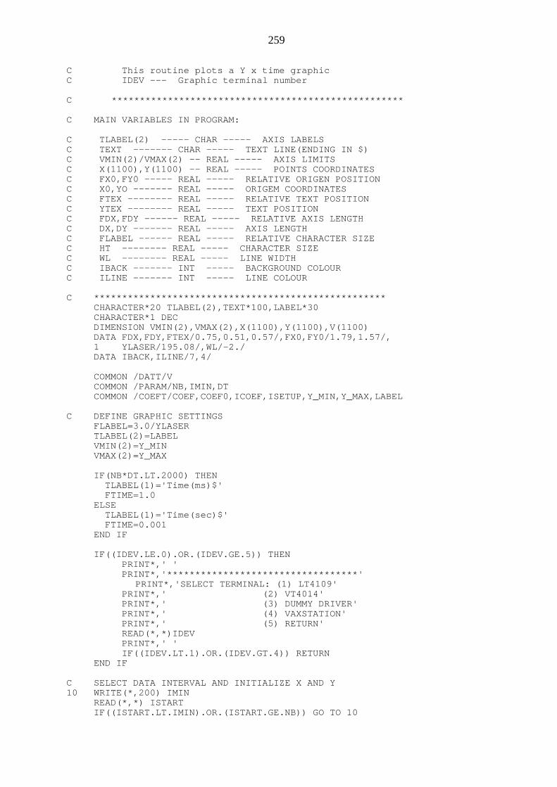
259
C This routine plots a Y x time graphicC IDEV --- Graphic terminal number
C ****************************************************
C MAIN VARIABLES IN PROGRAM:
C TLABEL(2) ----- CHAR ----- AXIS LABELSC TEXT ------- CHAR ----- TEXT LINE(ENDING IN $)C VMIN(2)/VMAX(2) -- REAL ----- AXIS LIMITSC X(1100),Y(1100) -- REAL ----- POINTS COORDINATESC FX0,FY0 ----- REAL ----- RELATIVE ORIGEN POSITIONC X0,YO ------- REAL ----- ORIGEM COORDINATESC FTEX -------- REAL ----- RELATIVE TEXT POSITIONC YTEX -------- REAL ----- TEXT POSITIONC FDX,FDY ------ REAL ----- RELATIVE AXIS LENGTHC DX,DY ------- REAL ----- AXIS LENGTHC FLABEL ------ REAL ----- RELATIVE CHARACTER SIZEC HT -------- REAL ----- CHARACTER SIZEC WL -------- REAL ----- LINE WIDTHC IBACK ------- INT ----- BACKGROUND COLOURC ILINE ------- INT ----- LINE COLOUR
C ****************************************************CHARACTER*20 TLABEL(2),TEXT*100,LABEL*30CHARACTER*1 DECDIMENSION VMIN(2),VMAX(2),X(1100),Y(1100),V(1100)DATA FDX,FDY,FTEX/0.75,0.51,0.57/,FX0,FY0/1.79,1.57/,1 YLASER/195.08/,WL/-2./DATA IBACK,ILINE/7,4/
COMMON /DATT/VCOMMON /PARAM/NB,IMIN,DTCOMMON /COEFT/COEF,COEF0,ICOEF,ISETUP,Y_MIN,Y_MAX,LABEL
C DEFINE GRAPHIC SETTINGSFLABEL=3.0/YLASERTLABEL(2)=LABELVMIN(2)=Y_MINVMAX(2)=Y_MAX
IF(NB*DT.LT.2000) THEN TLABEL(1)='Time(ms)$' FTIME=1.0ELSE TLABEL(1)='Time(sec)$' FTIME=0.001END IF
IF((IDEV.LE.0).OR.(IDEV.GE.5)) THEN PRINT*,' ' PRINT*,'**********************************'
PRINT*,'SELECT TERMINAL: (1) LT4109' PRINT*,' (2) VT4014' PRINT*,' (3) DUMMY DRIVER' PRINT*,' (4) VAXSTATION' PRINT*,' (5) RETURN' READ(*,*)IDEV PRINT*,' ' IF((IDEV.LT.1).OR.(IDEV.GT.4)) RETURNEND IF
C SELECT DATA INTERVAL AND INITIALIZE X AND Y10 WRITE(*,200) IMIN
READ(*,*) ISTARTIF((ISTART.LT.IMIN).OR.(ISTART.GE.NB)) GO TO 10
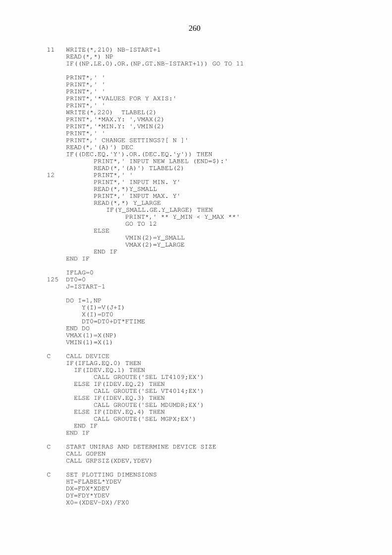
260
11 WRITE(*,210) NB-ISTART+1READ(*,*) NPIF((NP.LE.0).OR.(NP.GT.NB-ISTART+1)) GO TO 11
PRINT*,' 'PRINT*,' 'PRINT*,' 'PRINT*,'*VALUES FOR Y AXIS:'PRINT*,' 'WRITE(*,220) TLABEL(2)PRINT*,'*MAX.Y: ',VMAX(2)PRINT*,'*MIN.Y: ',VMIN(2)PRINT*,' 'PRINT*,' CHANGE SETTINGS?[ N ]'READ(*,'(A)') DECIF((DEC.EQ.'Y').OR.(DEC.EQ.'y')) THEN PRINT*,' INPUT NEW LABEL (END=$):' READ(*,'(A)') TLABEL(2)
12 PRINT*,' ' PRINT*,' INPUT MIN. Y' READ(*,*)Y_SMALL PRINT*,' INPUT MAX. Y' READ(*,*) Y_LARGE
IF(Y_SMALL.GE.Y_LARGE) THEN PRINT*,' ** Y_MIN < Y_MAX **' GO TO 12 ELSE VMIN(2)=Y_SMALL VMAX(2)=Y_LARGE END IFEND IF
IFLAG=0125 DT0=0
J=ISTART-1
DO I=1,NP Y(I)=V(J+I)
X(I)=DT0 DT0=DT0+DT*FTIMEEND DOVMAX(1)=X(NP)VMIN(1)=X(1)
C CALL DEVICEIF(IFLAG.EQ.0) THEN IF(IDEV.EQ.1) THEN
CALL GROUTE('SEL LT4109;EX') ELSE IF(IDEV.EQ.2) THEN CALL GROUTE('SEL VT4014;EX') ELSE IF(IDEV.EQ.3) THEN CALL GROUTE('SEL MDUMDR;EX') ELSE IF(IDEV.EQ.4) THEN CALL GROUTE('SEL MGPX;EX') END IFEND IF
C START UNIRAS AND DETERMINE DEVICE SIZECALL GOPENCALL GRPSIZ(XDEV,YDEV)
C SET PLOTTING DIMENSIONSHT=FLABEL*YDEVDX=FDX*XDEVDY=FDY*YDEVX0=(XDEV-DX)/FX0
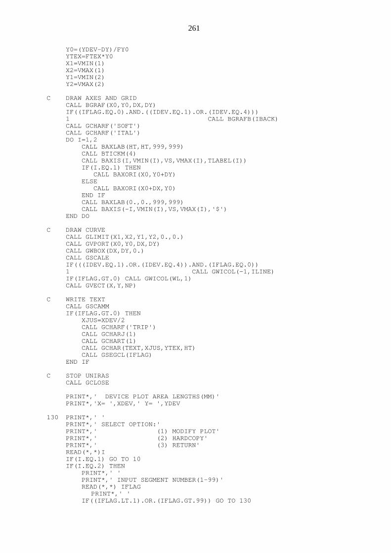
261
Y0=(YDEV-DY)/FY0YTEX=FTEX*Y0X1=VMIN(1)X2=VMAX(1)Y1=VMIN(2)Y2=VMAX(2)
C DRAW AXES AND GRIDCALL BGRAF(X0,Y0,DX,DY)IF((IFLAG.EQ.0).AND.((IDEV.EQ.1).OR.(IDEV.EQ.4)))1 CALL BGRAFB(IBACK)CALL GCHARF('SOFT')CALL GCHARF('ITAL')DO I=1,2 CALL BAXLAB(HT,HT,999,999) CALL BTICKM(4) CALL BAXIS(I,VMIN(I),VS,VMAX(I),TLABEL(I)) IF(I.EQ.1) THEN CALL BAXORI(X0,Y0+DY) ELSE CALL BAXORI(X0+DX,Y0) END IF CALL BAXLAB(0.,0.,999,999) CALL BAXIS(-I,VMIN(I),VS,VMAX(I),'$')END DO
C DRAW CURVECALL GLIMIT(X1,X2,Y1,Y2,0.,0.)CALL GVPORT(X0,Y0,DX,DY)CALL GWBOX(DX,DY,0.)CALL GSCALEIF(((IDEV.EQ.1).OR.(IDEV.EQ.4)).AND.(IFLAG.EQ.0))1 CALL GWICOL(-1,ILINE)IF(IFLAG.GT.0) CALL GWICOL(WL,1)CALL GVECT(X,Y,NP)
C WRITE TEXTCALL GSCAMMIF(IFLAG.GT.0) THEN XJUS=XDEV/2 CALL GCHARF('TRIP') CALL GCHARJ(1) CALL GCHART(1) CALL GCHAR(TEXT,XJUS,YTEX,HT) CALL GSEGCL(IFLAG)END IF
C STOP UNIRASCALL GCLOSE
PRINT*,' DEVICE PLOT AREA LENGTHS(MM)'PRINT*,'X= ',XDEV,' Y= ',YDEV
130 PRINT*,' 'PRINT*,' SELECT OPTION:'PRINT*,' (1) MODIFY PLOT'PRINT*,' (2) HARDCOPY'PRINT*,' (3) RETURN'READ(*,*)IIF(I.EQ.1) GO TO 10IF(I.EQ.2) THEN PRINT*,' ' PRINT*,' INPUT SEGMENT NUMBER(1-99)' READ(*,*) IFLAG
PRINT*,' ' IF((IFLAG.LT.1).OR.(IFLAG.GT.99)) GO TO 130
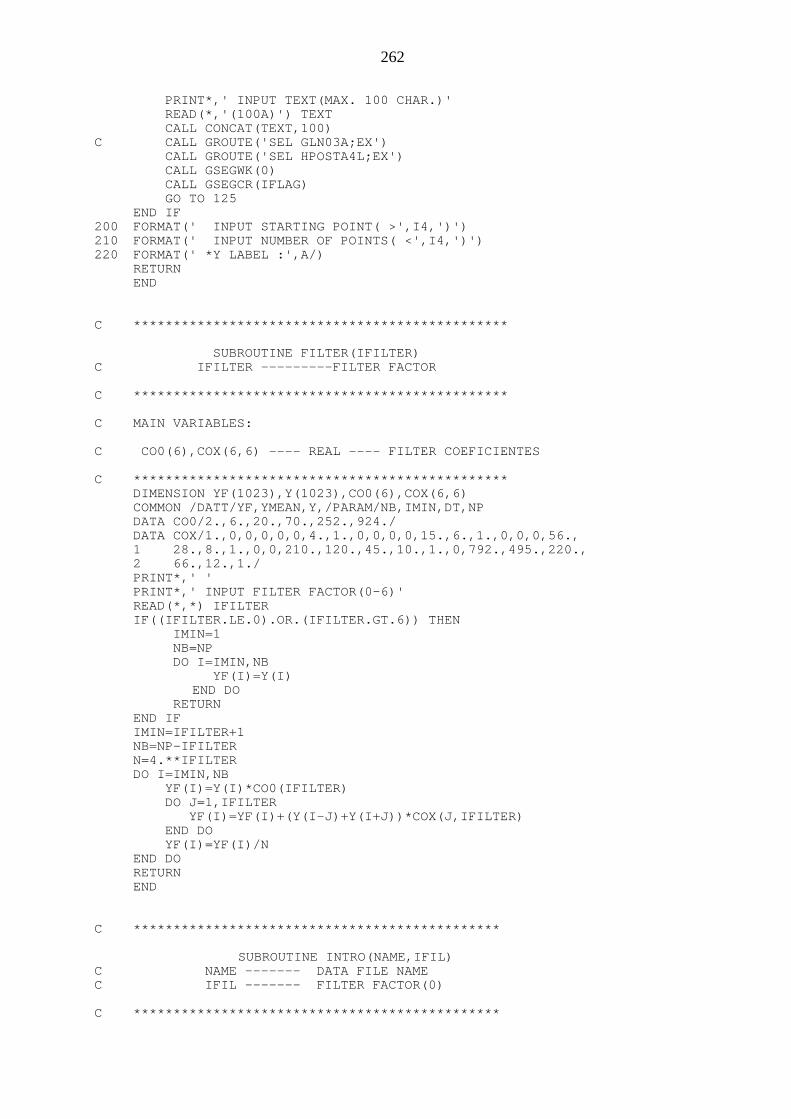
262
PRINT*,' INPUT TEXT(MAX. 100 CHAR.)' READ(*,'(100A)') TEXT CALL CONCAT(TEXT,100)
C CALL GROUTE('SEL GLN03A;EX') CALL GROUTE('SEL HPOSTA4L;EX') CALL GSEGWK(0) CALL GSEGCR(IFLAG) GO TO 125END IF
200 FORMAT(' INPUT STARTING POINT( >',I4,')')210 FORMAT(' INPUT NUMBER OF POINTS( <',I4,')')220 FORMAT(' *Y LABEL :',A/)
RETURNEND
C ***********************************************
SUBROUTINE FILTER(IFILTER)C IFILTER ---------FILTER FACTOR
C ***********************************************
C MAIN VARIABLES:
C CO0(6),COX(6,6) ---- REAL ---- FILTER COEFICIENTES
C ***********************************************DIMENSION YF(1023),Y(1023),CO0(6),COX(6,6)COMMON /DATT/YF,YMEAN,Y,/PARAM/NB,IMIN,DT,NPDATA CO0/2.,6.,20.,70.,252.,924./DATA COX/1.,0,0,0,0,0,4.,1.,0,0,0,0,15.,6.,1.,0,0,0,56.,1 28.,8.,1.,0,0,210.,120.,45.,10.,1.,0,792.,495.,220.,2 66.,12.,1./PRINT*,' 'PRINT*,' INPUT FILTER FACTOR(0-6)'READ(*,*) IFILTERIF((IFILTER.LE.0).OR.(IFILTER.GT.6)) THEN IMIN=1 NB=NP DO I=IMIN,NB YF(I)=Y(I)
END DO RETURNEND IFIMIN=IFILTER+1NB=NP-IFILTERN=4.**IFILTERDO I=IMIN,NB YF(I)=Y(I)*CO0(IFILTER) DO J=1,IFILTER YF(I)=YF(I)+(Y(I-J)+Y(I+J))*COX(J,IFILTER) END DO YF(I)=YF(I)/NEND DO
RETURNEND
C **********************************************
SUBROUTINE INTRO(NAME,IFIL)C NAME ------- DATA FILE NAMEC IFIL ------- FILTER FACTOR(0)
C **********************************************
263
CHARACTER*40 NAME,DEC*1,LABEL*30DIMENSION CF(1023),C(1023)COMMON /DATT/CF,CMEAN,CCOMMON /PARAM/NB,IMIN,DT,NP
C COMMON /COEFT/COEF,COEF0,ICOEF,ISETUP,Y_MIN,Y_MAX,LABEL
998 PRINT*,' 'PRINT*,' **************'PRINT*,' INPUT FILENAME'READ(*,'(A)') NAMEOPEN(UNIT=20,ERR=999,FILE=NAME,STATUS='OLD')READ(20,*) NB,DTREAD(20,*) (C(I),I=1,NB)CLOSE(20)
DO I=1,NB C(I)=CUVAL(C(I)) CF(I)=C(I)END DOIFIL=0IMIN=1NP=NBCMEAN=0RETURN
C ********************************************C ERROR DURING FILE OPENNING!!C ********************************************999 PRINT*,' ***THIS FILE CANNOT BE OPENED!***'
PRINT*,' DO YOU WANT TO TRY ANOTHER? (1)YES'PRINT*,' (2)NO'READ(*,*) IIF(I.EQ.1) GO TO 998
C ********************************************RETURNEND
C ************************************************
SUBROUTINE DISP
C ************************************************
DIMENSION CF(1023)COMMON/DATT/CF,/PARAM/NB,IMINPRINT*,' 'PRINT*,' FIRST AVAILABLE POINT:',IMINPRINT*,' LAST AVAILABLE POINT:',NB
10 PRINT*,' 'PRINT*,' INPUT LOWER LIMIT'READ(*,*) ILOWIF((ILOW.LT.IMIN).OR.(ILOW.GT.NB)) GO TO 10
20 PRINT*,' UPPER LIMIT'READ(*,*) IUPIF((IUP.LT.ILOW).OR.(IUP.GT.NB)) GO TO 20PRINT*,' 'WRITE(*,100) (CF(I),I=ILOW,IUP)
100 FORMAT(6F10.1)RETURNEND
C ************************************************************
264
SUBROUTINE PEAK(YPEAK,YBASE,YMAX,YMIN,NPEAK,NBASE,PER,PTIME)C YPEAK ---------------- PEAK CURRENT VALUESC YBASE ---------------- BASE CURRENT VALUESC YMAX ----------------- REFERENCE CURRENT(FOR YPEAK)C YMIN ----------------- " " (FOR YBASE)C NPEAK ---------------- NB OF PEAKSC NBASE ---------------- NB OF BASESC PER ------------------ MEAN PERIODC PTIME ---------------- PEAK TIMES
C ************************************************************
C MAIN VARIABLES:
C IIP(100) ---- INT ----- PEAK/BASE STARTING POINTSC IEP(100) ---- INT ----- PEAK/BASE ENDING POINTSC ************************************************************
DIMENSION YF(1023)DIMENSION IIP(100),IEP(100),YPEAK(100),YBASE(100),PTIME(100)COMMON /DATT/YF,YMEAN,/PARAM/NB,IMIN,DT
C SEARCH FOR PEAKS10 PRINT*,' '
PRINT*,' INPUT REFERENCE FOR PEAK CURRENT'READ(*,*) YMAXK=1CALL LIMIT(YMAX,N1,N2,K)IF(K.EQ.0) THEN PRINT*,' REFERENCE TOO LOW!' GO TO 10END IFCALL PEAKSEARCH(YMAX,N1,N2,IIP,IEP,NPEAK,1)IF(NPEAK.LE.1) GOTO 50PER=DT*(IIP(NPEAK)-IIP(1))/(NPEAK-1)DO I=1,NPEAK YPEAK(I)=YF(IIP(I)) PTIME(I)=DT*(IEP(I)-IIP(I)) DO J=IIP(I)+1,IEP(I) IF(YF(J).GT.YPEAK(I)) YPEAK(I)=YF(J) END DOEND DO
C SEARCH FOR BASE CURRENT VALUES30 PRINT*,' '
PRINT*,' INPUT REFERENCE FOR BASE CURENT'READ(*,*) YMINK=-1CALL LIMIT(YMIN,N1,N2,K)IF(K.EQ.0) THEN PRINT*,' REFERENCE TOO HIGH!' GO TO 30END IFCALL PEAKSEARCH(YMIN,N1,N2,IIP,IEP,NBASE,-1)IF(NBASE.LE.1) GO TO 50DO I=1,NBASE YBASE(I)=YF(IIP(I)) DO J=IIP(I)+1,IEP(I) IF(YF(J).LT.YBASE(I)) YBASE(I)=YF(J) END DOEND DOIF(NPEAK.EQ.0) THEN PRINT*,'TOO HIGH REFERENCE CUR. FOR PEAK CURRENT!' RETURNEND IF
50 RETURN
265
END
C *********************************************
SUBROUTINE LIMIT(YREF,ISTART,IEND,IFLAG)C YREF ---------- REFERENCE VALUEC ISTART -------- STARTING POINTC IEND ---------- FINNISHING POINTC IFLAG --------- RESULT FLAG
C *********************************************
DIMENSION YF(1023)COMMON /DATT/YF,/PARAM/NB,IMIN
REF=IFLAG*YREFK=IFLAGIFLAG=0DO I=IMIN,NB P1=K*YF(I) IF(P1.LT.REF) THEN ISTART=I IFLAG=1 GO TO 15
END IFEND DOIF(IFLAG.EQ.0) GO TO 30
15 DO I=IMIN,NB J=NB-I+1 P1=K*YF(J) IF(P1.LT.REF) THEN IEND=J GO TO 30 END IFEND DO
30 RETURNEND
C *************************************************
SUBROUTINE CREATEC THIS ROUTINE SAVES DATA IN FILE
C *************************************************
CHARACTER*40 NOME,VARIABLEDIMENSION DADO(1023)COMMON /DATT/DADO,/PARAM/NB,IMIN,DT
PRINT*,' INPUT NAME OF FILE TO BE CREATED'READ(*,'(A)') NOMEPRINT*,' INPUT VARIABLE NAME(END=$)'READ(*,'(A)') VARIABLEOPEN(UNIT=15,FILE=NOME,STATUS='NEW')I=NB-IMIN+1WRITE(15,*) I,DTWRITE(15,100) (DADO(I),I=IMIN,NB)WRITE(15,'(A)') VARIABLECLOSE(15)RETURN
100 FORMAT(7F10.1)END
266
C ************************************************
SUBROUTINE REPORT(I)
C ************************************************
CHARACTER*1 NAMEI=0PRINT*,' DO YOU WANT TO SAVE THESE DATA? (Y/y)YES'PRINT*,' (N/n)NO'READ(*,'(1A)') NAMEIF((NAME.EQ.'Y').OR.(NAME.EQ.'y')) I=1RETURNEND
C ************************************************** FUNCTION CUVAL(X)
C **************************************************
COMMON /COEFT/FT,F0IF(X.LT.128) X=128.IF(X.GT.255) X=256CUVAL=FT*(X-128.)+F0RETURNEND
C ******************************************************
SUBROUTINE STATS(DAT,IMIN,NUB,YMEAN,STD,YEFF)C DAT(1100)--------- DATAC IMIN ------------- FIRST POINT NBC NUB -------------- NUMBER OF POINTSC YMEAN ------------ MEAN(999.9 -> ERROR CONDITION)C STD -------------- ST. DEV.(999.9 -> ERROR CONDITION)C YEFF ------------- EFFECTIVE MEANC ******************************************************
DIMENSION DAT(1100)IF(NUB.LE.1) THEN YMEAN=-999.9 STD=-999.9 RETURNELSE IMAX=IMIN+NUB-1 YMEAN=0 STD=0END IFDO I=IMIN,IMAX YMEAN=YMEAN+DAT(I)END DOYMEAN=YMEAN/NUBDO I=IMIN,IMAX STD=STD+(DAT(I)-YMEAN)**2END DOSTD=SQRT(STD/(NUB-1))IF(YEFF.NE.0) THEN YEFF=0 DO I=IMIN,IMAX YEFF=YEFF+DAT(I)*DAT(I) END DO YEFF=SQRT(YEFF/NUB)END IFRETURNEND
267
C *****************************************************
SUBROUTINE PEAKSEARCH(YREF,N1,N2,ISTART,IEND,NV,ISIG)C YREF ---------- REFERENCE VALUEC N1 ------------ FIRST POINTC N2 ------------ LAST POINTC ISTART(100) --- PEAK/BASE STARTING POINTC IEND(100) ----- PEAK/BASE FINNISHING POINTC NV ------------ NUMBER OF PEAKS/BASESC ISIG ----------( 1) -> PEAKC (-1) -> BASE
C *****************************************************
DIMENSION DAT(1023)DIMENSION ISTART(100),IEND(100)
COMMON /DATT/DAT
IFLAG=0NV=0REF=ISIG*YREFDO 10 I=N1,N2 YTEST=ISIG*DAT(I) IF((YTEST.GT.REF).AND.(IFLAG.EQ.0)) THEN NV=NV+1 IFLAG=1 ISTART(NV)=I GO TO 10 END IF IF(IFLAG.EQ.0) GO TO 10 IF(YTEST.LT.REF) THEN IFLAG=0 IEND(NV)=I END IF
10 CONTINUERETURNEND
C **************************************************
SUBROUTINE PAREA(AREA,YREF,NV)C AREA(100) ----------- PEAK AREASC YREF ------------- REFERENCE CURRENTC NV -------------- NUMBER OF PEAKS
C **************************************************
DIMENSION DAT(1023)DIMENSION IIP(100),IEP(100),AREA(100)COMMON /DATT/DAT,/PARAM/NB,IMIN,DT
10 PRINT*,' 'PRINT*,' INPUT REFERENCE CURRENT'READ(*,*) YREFK=1CALL LIMIT(YREF,N1,N2,K)IF(K.EQ.0) THEN PRINT*,' REFERENCE TOO LOW!' GO TO 10END IFCALL PEAKSEARCH(YREF,N1,N2,IIP,IEP,NV,1)IF(NV.LE.1) GO TO 40
268
DO 30 I=1,NV AREA(I)=0 DO 20 J=IIP(I),IEP(I) AREA(I)=AREA(I)+2.*DAT(J)
20 CONTINUE AREA(I)=DT/2000.*(AREA(I)-DAT(IIP(I))-DAT(IEP(I)))
30 CONTINUE40 RETURN
END
C *******************************************************
SUBROUTINE BOUND(DATA,IDIM,NP,IMIN,VMAX,VMIN)
C *******************************************************
DIMENSION DATA(IDIM)VMAX=DATA(IMIN)VMIN=DATA(IMIN)DO I=IMIN+1,IMIN+NP-1 IF(DATA(I).GT.VMAX) VMAX=DATA(I) IF(DATA(I).LT.VMIN) VMIN=DATA(I)END DORETURNEND
C *******************************************************
SUBROUTINE CONCAT(XIN,N)
C *******************************************************
CHARACTER*100 XIN,XOUTI=N+1
10 I=I-1IF(I.EQ.0)THEN I=1ELSE IF(XIN(I:I).EQ.' ')GOTO 10END IFXOUT=XIN(:I)//'$'XIN=XOUTRETURNEND
C *******************************************************
SUBROUTINE SET_UP
C *******************************************************
COMMON /COEFT/COEF,COEF0,ICOEF,ISETUP,Y_MIN,Y_MAX,LABELCHARACTER*30 LABEL,NAME,DEC*1,DEC1*1,DEC2*1
PRINT*,' 'PRINT*,'*CALIBRATION FACTORS :'PRINT*,'*'PRINT*,'*SLOPE : ',COEFPRINT*,'*INTERCEPT: ',COEF0PRINT*,'*'PRINT*,'*Y_MIN : ',Y_MIN

269
PRINT*,'*Y_MAX : ',Y_MAX PRINT*,'*'
WRITE(*,100)LABEL
PRINT*,' 'PRINT*,' CHANGE CALIBRATION COEFICIENTS?[N]'
READ(*,'(A)')DECIF((DEC.EQ.'Y').OR.(DEC.EQ.'y')) THEN PRINT*,' ' PRINT*,' READ SET UP FROM FILE? [N]' READ(*,'(A)') DEC1 PRINT*,' ' IF((DEC1.EQ.'Y').OR.(DEC1.EQ.'y')) THEN PRINT*,' INPUT FILE NAME:' READ(*,'(A)') NAME OPEN(UNIT=20,ERR=999,FILE=NAME,STATUS='OLD') READ(20,*) COEF,COEF0 READ(20,*) Y_MIN,Y_MAX READ(20,'(A)') LABEL CLOSE(20) PRINT*,' ** DONE! **' ELSE PRINT*,' INPUT NEW SLOPE' READ(*,*)COEF PRINT*,' INPUT NEW INTERCEPT' READ(*,*) COEF0 PRINT*,'CHANGE Y LABEL?(Y/N)'
READ(*,'(A)') DEC2 IF((DEC2.EQ.'Y').OR.(DEC2.EQ.'y')) THEN PRINT*,' INPUT NEW LABEL FOR Y (END $)' READ(*,'(A)')LABEL
END IF10 PRINT*,' '
PRINT*,' CHANGE MAXIMUN AND MINUMUM VALUES OF' PRINT*,' Y(FOR PLOTTING)?(Y/N)'
READ(*,'(A)')DEC IF((DEC.EQ.'Y').OR.(DEC.EQ.'y')) THEN PRINT*,' INPUT YMIN' READ(*,*)Y_SMALL PRINT*,' INPUT YMAX' READ(*,*) Y_LARGE
IF(Y_SMALL.GE.Y_LARGE) THEN PRINT*,' ** Y_MIN < Y_MAX **' GO TO 10 ELSE Y_MIN=Y_SMALL Y_MAX=Y_LARGE END IF END IF END IF ISETUP=1 ICOEF=1ELSE ISETUP=0 ICOEF=0END IFRETURN
999 PRINT*,' ********* CANNOT OPEN SETUP FILE! ***********'PRINT*,' 'RETURN
100 FORMAT(' *Y LABEL :',2X,A/)END

APPENDIX C

271
This appendix exemplifies the use of the SPSSx language to write programmes for statisticalmodelling.
A)PROGRAMME:
TITLE REGRESSION MODELS-HE2+O2 HORIZ. WELDINGFILE HANDLE MODEL NAME='[IS931.MATH2]MODEHOR.DAT'DATA LIST FILE=MODEL LIST / WFR IARC SPEED Y1 TO Y8COMPUTE Y9=Y6*SPEEDCOMPUTE Y10=Y2-(Y3+Y4)DO REPEAT Y=Y1 TO Y10/L=LY1 TO LY10. COMPUTE L=LN(Y)END REPEATDO REPEAT Y=Y1 TO Y10/R=RY1 TO RY10. COMPUTE R=1./YEND REPEATVARIABLE LABELS Y2 'BEAD AREA(MM2) - At' Y3 'DEPOSITED AREA(MM2) - Ad' Y4 'LAT. PEN. AREA(MM2) - Ap' Y5 'LAT. PEN.(MM) - p' Y6 'MEAN HEIGHT(MM) - h' Y7 'HEIGHT/WIDTH RATIO - R' Y8 'Aau/Aal - Ralu' Y9 'PRODUCTIVITY(MM2/S) - tp' Y1 'ARC VOLTAGE(V)' Y10 'AXIAL PENETRATION AREA - Aa' LY2 'LN(At)' LY3 'LN(Ad)' LY4 'LN(Ap)' LY5 'LN(p)' LY6 'LN(h)' LY7 'LN(R)' LY8 'LN(Ralu)' LY9 'LN(tp)' LY1 'LN(V)' LY10 'LN(Aa)' RY2 'INV(At)' RY3 'INV(Ad)' RY4 'INV(Ap)' RY5 'INV(p)' RY6 'INV(h)' RY7 'INV(R)' RY8 'INV(Ralu)' RY9 'INV(tp)' RY1 'INV(V)' RY10 'INV(Aa)' WFR 'W. F. R.(M/MIN)' SPEED 'WELD. SPEED(MM/S)' IARC 'CURRENT(A)'DESCRIPTIVES VARIABLES= IARC WFR SPEED /SAVEREGRESSION DESCRIPTIVES=DEFAULTS/ VARS= ZIARC ZWFR ZSPEED Y1 TO Y10/ STATISTICS=DEFAULTS CI/ DEP=Y1 TO Y10/BACKWARD/ CASEWISE=DEFAULTS/ SCATTERPLOT (*RES,*PRE)/REGRESSION DESCRIPTIVES=DEFAULTS/ VARS= ZIARC ZWFR ZSPEED LY1 TO LY10/ STATISTICS=DEFAULTS CI/ DEP=LY1 TO LY10/BACKWARD/ CASEWISE=DEFAULTS/ SCATTERPLOT (*RES,*PRE)/REGRESSION DESCRIPTIVES=DEFAULTS/ VARS= ZIARC ZWFR ZSPEED RY1 TO RY10/ STATISTICS=DEFAULTS CI/ DEP=RY1 TO RY10/BACKWARD/ CASEWISE=DEFAULTS/ SCATTERPLOT (*RES,*PRE)/

272
COMPUTE IXW=ZIARC*ZWFRCOMPUTE IXS=ZIARC*ZSPEEDCOMPUTE WXS=ZWFR*ZSPEEDREGRESSION DESCRIPTIVES=DEFAULTS/ VARS=ZIARC ZWFR ZSPEED IXW IXS WXS Y1 TO Y10/ STATISTICS=DEFAULTS CI/ DEP=Y1 TO Y10/STEPWISE/ CASEWISE=DEFAULTS/ SCATTERPLOT (*RES,*PRE)/REGRESSION DESCRIPTIVES=DEFAULTS/ VARS=ZIARC ZWFR ZSPEED IXW IXS WXS LY1 TO LY10/ STATISTICS=DEFAULTS CI/ DEP=LY1 TO LY10/STEPWISE/ CASEWISE=DEFAULTS/ SCATTERPLOT (*RES,*PRE)/REGRESSION DESCRIPTIVES=DEFAULTS/ VARS=ZIARC ZWFR ZSPEED IXW IXS WXS RY1 TO RY10/ STATISTICS=DEFAULTS CI/ DEP=RY1 TO RY10/STEPWISE/ CASEWISE=DEFAULTS/ SCATTERPLOT (*RES,*PRE)/FINISH
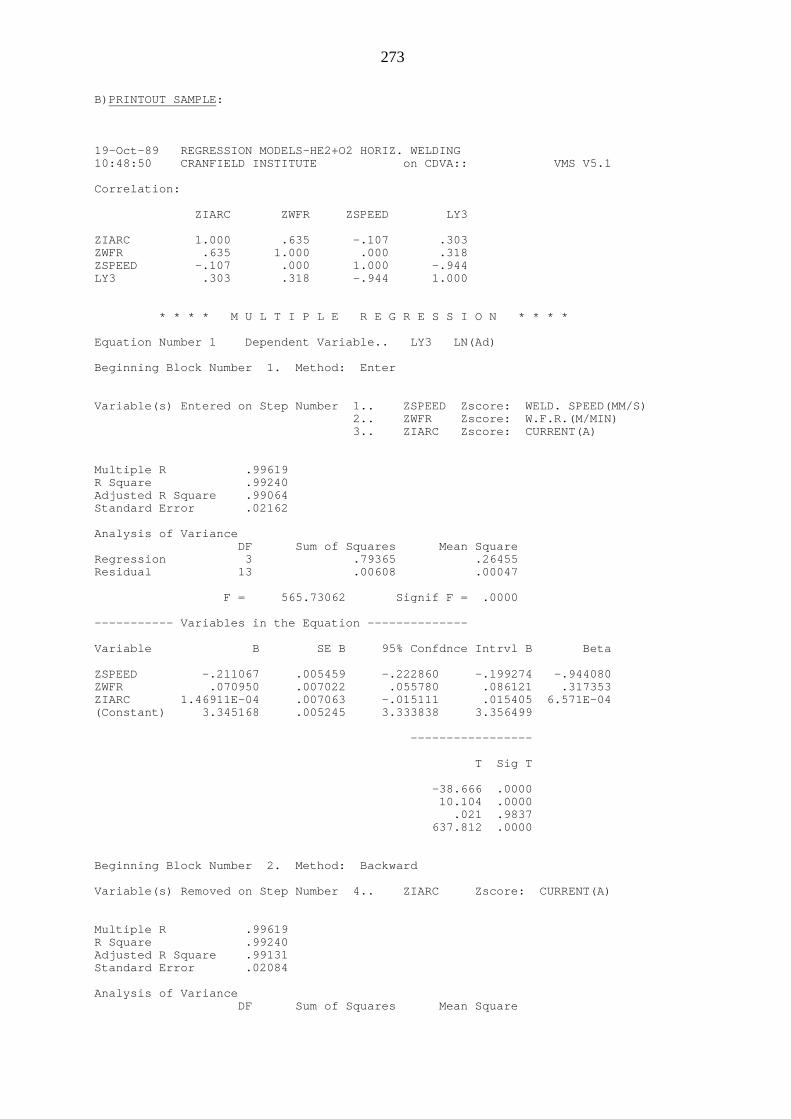
273
B)PRINTOUT SAMPLE:
19-Oct-89 REGRESSION MODELS-HE2+O2 HORIZ. WELDING10:48:50 CRANFIELD INSTITUTE on CDVA:: VMS V5.1
Correlation:
ZIARC ZWFR ZSPEED LY3
ZIARC 1.000 .635 -.107 .303ZWFR .635 1.000 .000 .318ZSPEED -.107 .000 1.000 -.944LY3 .303 .318 -.944 1.000
* * * * M U L T I P L E R E G R E S S I O N * * * *
Equation Number 1 Dependent Variable.. LY3 LN(Ad)
Beginning Block Number 1. Method: Enter
Variable(s) Entered on Step Number 1.. ZSPEED Zscore: WELD. SPEED(MM/S) 2.. ZWFR Zscore: W.F.R.(M/MIN) 3.. ZIARC Zscore: CURRENT(A)
Multiple R .99619R Square .99240Adjusted R Square .99064Standard Error .02162
Analysis of Variance DF Sum of Squares Mean SquareRegression 3 .79365 .26455Residual 13 .00608 .00047
F = 565.73062 Signif F = .0000
----------- Variables in the Equation --------------
Variable B SE B 95% Confdnce Intrvl B Beta
ZSPEED -.211067 .005459 -.222860 -.199274 -.944080ZWFR .070950 .007022 .055780 .086121 .317353ZIARC 1.46911E-04 .007063 -.015111 .015405 6.571E-04(Constant) 3.345168 .005245 3.333838 3.356499
-----------------
T Sig T
-38.666 .0000 10.104 .0000 .021 .9837 637.812 .0000
Beginning Block Number 2. Method: Backward
Variable(s) Removed on Step Number 4.. ZIARC Zscore: CURRENT(A)
Multiple R .99619R Square .99240Adjusted R Square .99131Standard Error .02084
Analysis of Variance DF Sum of Squares Mean Square
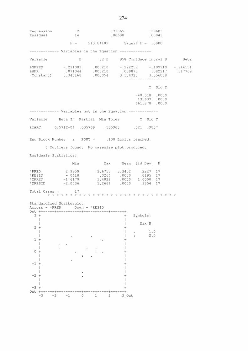
274
Regression 2 .79365 .39683Residual 14 .00608 .00043
F = 913.84189 Signif F = .0000
------------- Variables in the Equation --------------
Variable B SE B 95% Confdnce Intrvl B Beta
ZSPEED -.211083 .005210 -.222257 -.199910 -.944151ZWFR .071044 .005210 .059870 .082217 .317769(Constant) 3.345168 .005054 3.334328 3.356008 -----------------
T Sig T
-40.518 .0000 13.637 .0000 661.878 .0000
------------- Variables not in the Equation -------------
Variable Beta In Partial Min Toler T Sig T
ZIARC 6.571E-04 .005769 .585908 .021 .9837
End Block Number 2 POUT = .100 Limits reached.
0 Outliers found. No casewise plot produced.
Residuals Statistics:
Min Max Mean Std Dev N
*PRED 2.9850 3.6753 3.3452 .2227 17*RESID -.0418 .0264 .0000 .0195 17*ZPRED -1.6170 1.4822 .0000 1.0000 17*ZRESID -2.0036 1.2664 .0000 .9354 17
Total Cases = 17 * * * * * * * * * * * * * * * * * * * * * * * * * * * * *
Standardized ScatterplotAcross - *PRED Down - *RESIDOut ++-----+-----+-----+-----+-----+-----++ 3 + + Symbols: | | | | Max N 2 + + | | . 1.0 | . . | : 2.0 1 + . + | . . | | . . . | 0 + . . . + | : . | | . | -1 + + | | | . | -2 + . + | | | | -3 + +Out ++-----+-----+-----+-----+-----+-----++ -3 -2 -1 0 1 2 3 Out