Creating a Visual, Interactive

Representation of Traffic Flow

Eric Mai • CE 291F • May 4, 2009

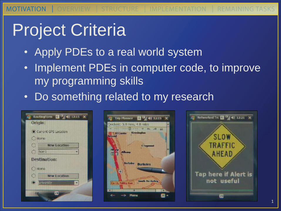
Project Criteria • Apply PDEs to a real world system

• Implement PDEs in computer code, to improve

my programming skills

• Do something related to my research

1

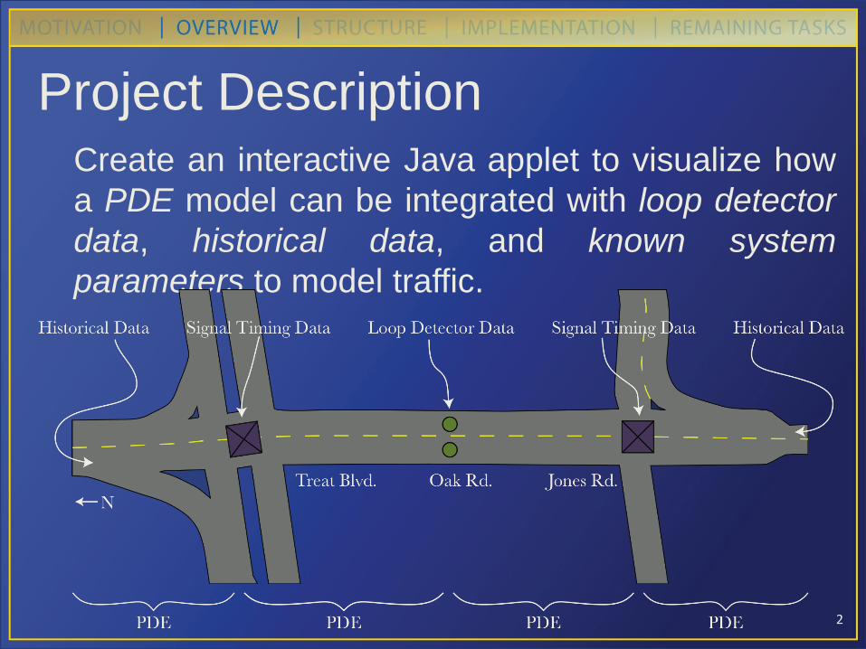
Create an interactive Java applet to visualize how

a PDE model can be integrated with loop detector

data, historical data, and known system

parameters to model traffic.

2

Project Description

3

4

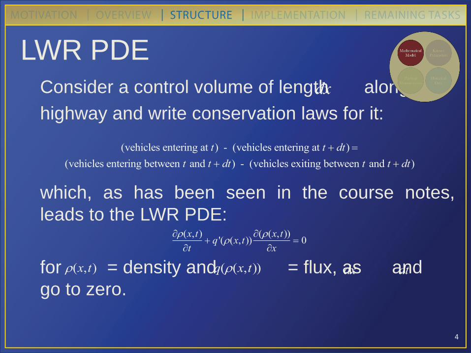
LWR PDE Consider a control volume of length along a

highway and write conservation laws for it:

which, as has been seen in the course notes,

leads to the LWR PDE:

for = density and = flux, as and

go to zero.

dx

(vehicles entering at t) - (vehicles entering at t dt)

(vehicles entering between t and t dt) - (vehicles exiting between t and t dt)

(x,t)

t q '((x,t))

((x,t))

x 0

(x,t) q((x,t)) dx dt

5

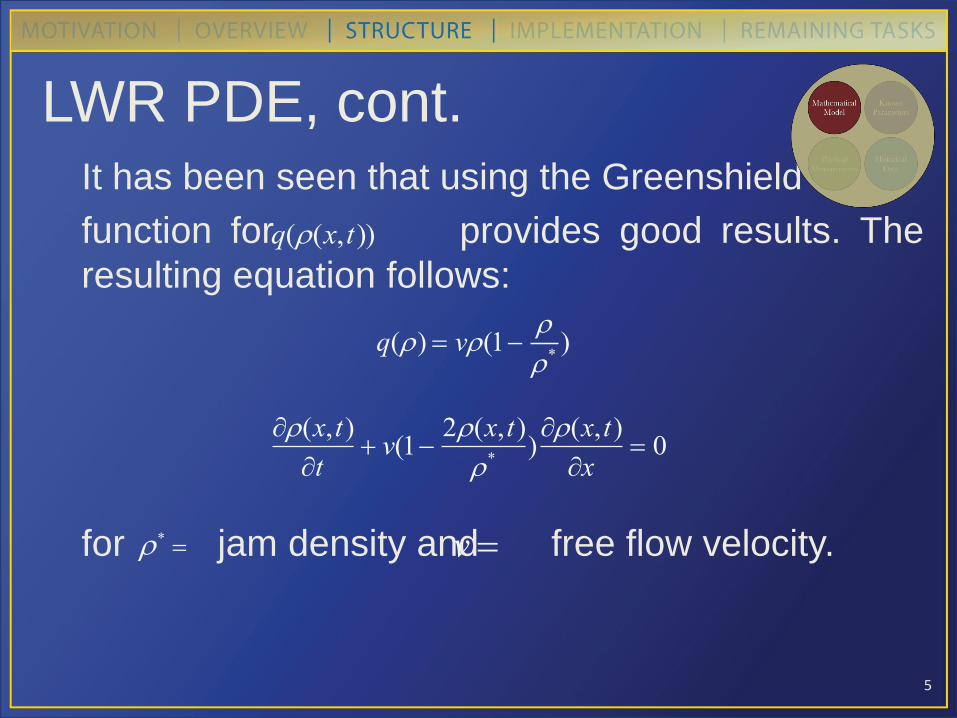
LWR PDE, cont. It has been seen that using the Greenshield flux

function for provides good results. The

resulting equation follows:

for jam density and free flow velocity.

q((x,t))

q() v(1

*)

(x,t)

t v(1

2(x,t)

*)(x,t)

x 0

* v

6

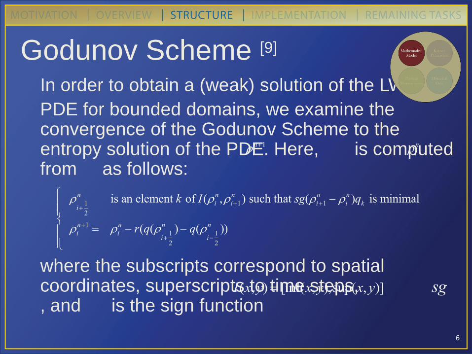
Godunov Scheme [9]

In order to obtain a (weak) solution of the LWR

PDE for bounded domains, we examine the convergence of the Godunov Scheme to the entropy solution of the PDE. Here, is computed from as follows:

where the subscripts correspond to spatial coordinates, superscripts to time steps, , and is the sign function

in1 i

n

i

1

2

n is an element k of I(in ,i1

n ) such that sg(i1

n in )qk is minimal

in1 i

n r(q(i

1

2

n ) q(i

1

2

n ))

I(x,y) [inf(x,y),sup(x,y)] sg

7

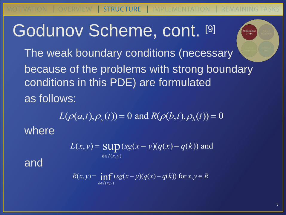
Godunov Scheme, cont. [9]

The weak boundary conditions (necessary

because of the problems with strong boundary

conditions in this PDE) are formulated

as follows:

where

and

L((a,t),a(t)) 0 and R((b,t),b(t)) 0

L(x, y) kI (x,y)

sup (sg(x y)(q(x) q(k)) and

R(x, y) kI (x,y)inf (sg(x y)(q(x) q(k)) for x, yR

8

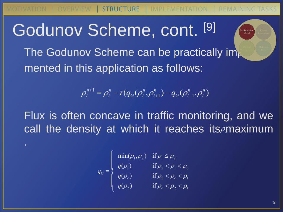
Godunov Scheme, cont. [9] The Godunov Scheme can be practically imple-

mented in this application as follows:

Flux is often concave in traffic monitoring, and we

call the density at which it reaches its maximum

.

in1 i

n r(qG(in,i1

n ) qG(i1

n ,in )

c

qG

min(1,2 ) if 1 2

q(1) if 2 1 c

q(c ) if 2 c 1

q(2 ) if c 2 1

9

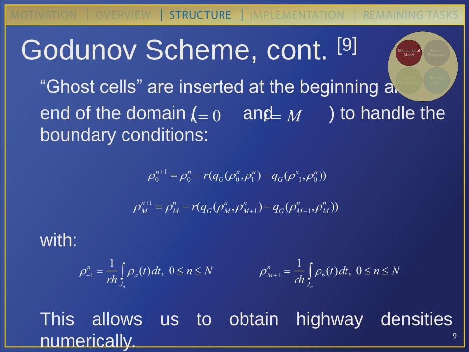
Godunov Scheme, cont. [9] “Ghost cells” are inserted at the beginning and

end of the domain ( and ) to handle the

boundary conditions:

with:

This allows us to obtain highway densities

numerically.

i 0 i M

0

n1 0

n r(qG(0

n,1

n ) qG(1

n ,0

n ))

Mn1 M

n r(qG(Mn ,M 1

n ) qG(M 1

n ,Mn ))

1

n 1

rha(t)dt, 0 n N

Jn

M 1

n 1

rhb(t)dt, 0 n N

Jn

10

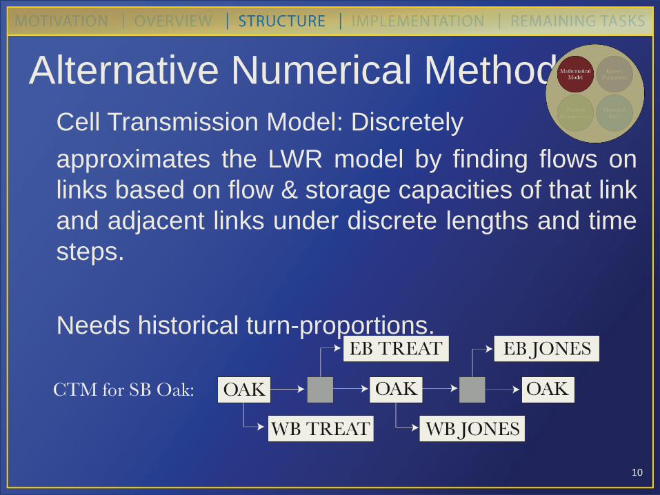
Alternative Numerical Method [2]

Cell Transmission Model: Discretely

approximates the LWR model by finding flows on

links based on flow & storage capacities of that link

and adjacent links under discrete lengths and time

steps.

Needs historical turn-proportions.

11

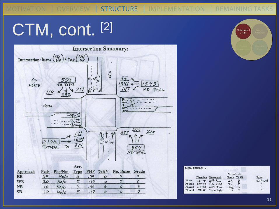
CTM, cont. [2]

12

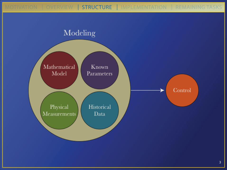
Known System Parameters Need boundary conditions and physical

characteristics of system for PDEs to work:

• Signal timing

• Lane configuration

• Expected turning proportions (for CTM)

Physical Measurements • Loop detector data – detect changes in the

system and inform the PDEs (boundary

conditions)

13

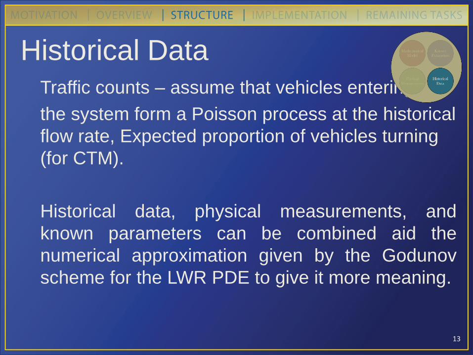
Historical Data Traffic counts – assume that vehicles entering

the system form a Poisson process at the historical

flow rate, Expected proportion of vehicles turning

(for CTM).

Historical data, physical measurements, and

known parameters can be combined aid the

numerical approximation given by the Godunov

scheme for the LWR PDE to give it more meaning.

14

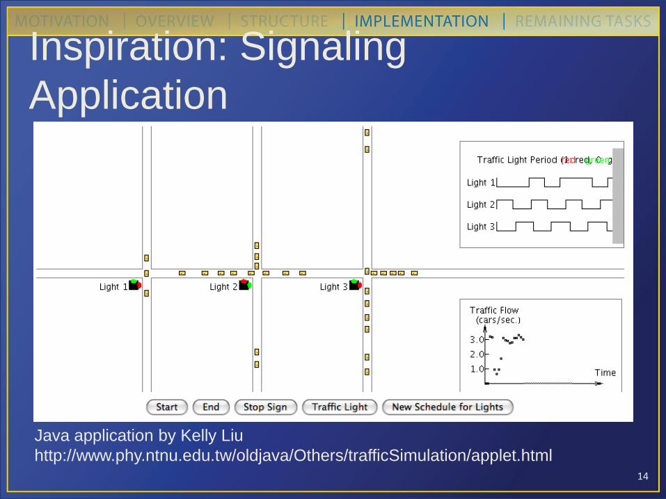
Inspiration: Signaling

Application

Java application by Kelly Liu

http://www.phy.ntnu.edu.tw/oldjava/Others/trafficSimulation/applet.html

15

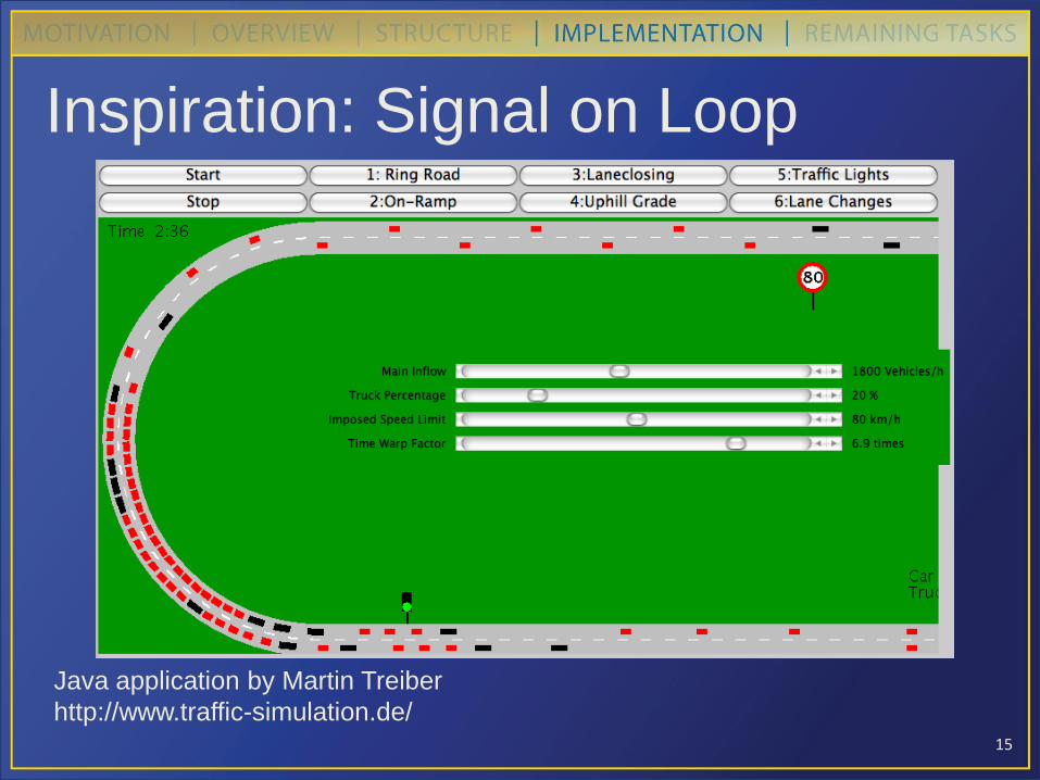
Inspiration: Signal on Loop

Java application by Martin Treiber

http://www.traffic-simulation.de/

16

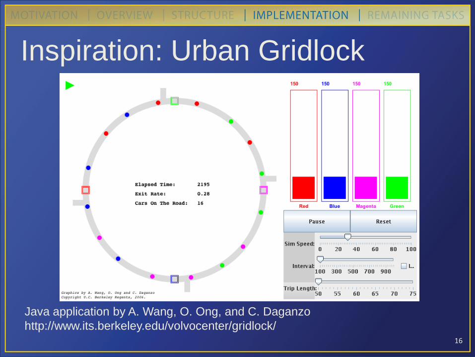
Inspiration: Urban Gridlock

Java application by A. Wang, O. Ong, and C. Daganzo

http://www.its.berkeley.edu/volvocenter/gridlock/

17

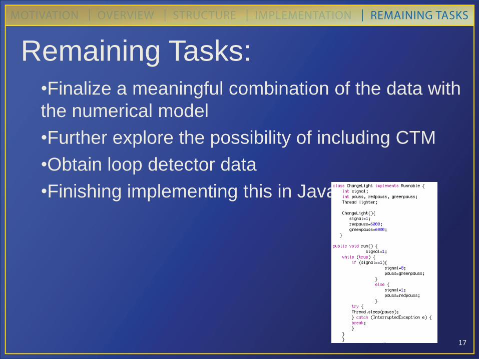
Remaining Tasks: •Finalize a meaningful combination of the data with

the numerical model

•Further explore the possibility of including CTM

•Obtain loop detector data

•Finishing implementing this in Java

18

References 1. C.G. Claudel, A. Hofleitner, N. Mignerey and A. M. Bayen. Guaranteed bounds on highway travel

times using probe and fixed data. To appear in the 88th TRB Annual Meeting Compendium of

Papers DVD, Washington D.C., January 11-15 2009. Transportation Research Board.

2. Daganzo, Carlos F., The Cell Transmission Model: Network Traffic, California PATH, 1994.

3. Hong K. Lo, A novel traffic signal control formulation, Transportation Research Part A: Policy and

Practice, Volume 33, Issue 6, August 1999, Pages 433-448, ISSN 0965-8564, DOI:

10.1016/S0965-8564(98)00049-4.

4. J. C. Herrera and A. M. Bayen. Eulerian versus Lagrangian Sensing in Traffic State Estimation. To

appear in the 18th symposium on Transportation and Traffic Theory, Hong Kong, 2009.

5. J.C. Herrera and A. M. Bayen. Traffic flow reconstruction using mobile sensors and loop detector

data. In 87th TRB Annual Meeting Compendium of Papers DVD, Washington D.C., January 13-17

2008. Transportation Research Board.

6. Jun-Seok Oh, R. Jayakrishnan, and Will Recker, "Section Travel Time Estimation from Point

Detection Data" (August 1, 2002). Center for Traffic Simulation Studies. Paper UCI-ITS-TS-WP-

02-15.

7. Lo, H.K.; Chan, Y.C.; Chow, A.H.F., "A new dynamic traffic control system: performance of adaptive

control strategies for over-saturated traffic," Intelligent Transportation Systems, 2001.

Proceedings. 2001 IEEE , vol., no., pp.404-409, 2001

8. Lin, W.H., Ahanotu, D., 1995. Validating the basic cell transmission model on a single freeway link.

University of California, Berkeley. Technical Note, UCB-ITS-PATH-TN-95-3.

9. Strub, I and A. Bayen, "Mixed Initial-boundary Value Problems for Scalar Conservation Laws:

Application to the Modeling of Transportation Networks," Hybrid Systems: Computation and

Cotnrol (J. Hespanha, A. Tiwari, Eds), Lecture Notes in Computer Science 3927, Springer-Verlag,

March 2006, pp. 552-567.