Credit Contagion from Counterparty Risk

Philippe Jorion*

and

Gaiyan Zhang**

* Paul Merage School of Business, University of California at Irvine ** College of Business Administration, University of Missouri at St. Louis The paper has benefited from comments and suggestions from participants at the NBER Conference on the Risk of Financial Institutions and the FDIC's Center for Financial Research Workshop, and from Richard Cantor, Vicente Cunat, Sanjiv Das, Kay Giesecke, Jean Helwege, Robert A. Jarrow, as well as the editor. We thank the Markit Group Limited for providing the CDS data. Gaiyan Zhang gratefully acknowledges the financial support from the FDIC's Center for Financial Research.

Correspondence can be addressed to:

Philippe Jorion Paul Merage School of Business University of California at Irvine Irvine, CA 92697-3125 Phone: (949) 824-5245, E-mail: pjorion@uci.edu

Gaiyan Zhang College of Business Administration University of Missouri St. Louis, MO 63121, USA Phone: (636) 516-6269 E-mail: zhangga@umsl.edu

1

Credit Contagion from Counterparty Risk

Abstract

Standard credit risk models cannot explain the observed clustering of default, sometimes described as “credit contagion.” This paper provides the first empirical analysis of credit contagion via direct counterparty effects. We examine the wealth effects of bankruptcy announcements on creditors using a unique database. On average, creditors experience severe negative abnormal equity returns and increases in CDS spreads. In addition, creditors are more likely to suffer from financial distress later. These effects are stronger for industrial creditors than financials. Simulations calibrated to these results indicate that counterparty risk can potentially explain the observed excess clustering of defaults. This suggests that counterparty risk is an important additional channel of credit contagion and that current portfolio credit risk models understate the likelihood of large losses.

1

Portfolio credit risk models have vastly improved in recent years, allowing financial

institutions to measure their distribution of their potential credit losses at the top level of the

institution. Such information can be used to infer economic capital, which is the amount of equity

capital the institution should carry to absorb a large loss over a specified horizon with a high

confidence level. These new credit models are now in widespread use in the financial industry, for

instance when structuring Collateralized Debt Obligations (CDOs).1 These models are also the

basis for the recently-established regulatory capital charges for commercial banks.2

There are, however, nagging concerns about the calibration of these models. In particular,

estimation of default correlations is difficult because they cannot be directly measured for specific

obligors. In addition, current models for default correlations seem to be unable to reproduce the

actual pattern of default clustering, sometimes called “credit contagion”. This paper provides an

empirical analysis of an important channel of credit contagion, which is counterparty credit risk.

Unexplained default clustering is a major issue for traditional credit risk models because it

generates greater dispersion in the distribution of credit losses. This implies a greater likelihood of

large losses and an understatement of economic capital. This could lead to a greater number of

bank failures in periods of stress, or losses on CDOs that exceed worst estimates. Indeed, losses on

CDOs backed by subprime debt have been at the heart of the financial crisis that started in 2007.

In traditional credit models default correlations are inferred from a structural model of the

value of the firm or by a reduced-form model of default intensity. A typical simplification uses

factor models, where correlations are induced by a common factor that can be interpreted as the

state of the economy, plus possibly other factors. Das et al. (2007) indicate that the conditionally

1 The CDO market has experienced exponential growth in recent years, with more than $550 billion in new issues in 2006 alone. 2 These new rules, called Basel II, impose minimum levels of capital that commercial banks have to hold to guard against credit and other risks. The credit risk charge roughly corresponds to the worst credit loss over a one-year horizon at the 99.9 percent level of confidence.

2

independent assumption for factor models forms the current basis of credit risk management

practice. Indeed, the new Basel II regulatory capital charges are based on such factor models.3 This

common feature largely explains why recent comparative studies of industry portfolio models show

remarkable similarities in their outputs, or measures of economic capital.4 Such models, however,

do not fully capture the clustering in default correlations reported, for instance, in Das et al. (2007).5

Second-generation models attempt to provide structural explanations for this default

clustering. For instance, Duffie et al. (2006) estimate a “frailty” model where defaults are driven by

an unobserved time-varying latent variable, which partially explains the observed default clustering.

Another extension would be to consider multiple factor effects, or industry factors. When a firms

defaults, other firms in the same industry could suffer from contagion effects, reflecting shocks to

cash flows that are common to that industry. Examining firms within the same industry, Lang and

Stulz (1992) and Jorion and Zhang (2007) present evidence that industry peers are negatively

affected by a firm’s Chapter 11 bankruptcy, creating higher correlation within the industry. The

recent upheaval in securities backed by subprime mortgage debt indicates that the financial industry

indeed has missed major common default factors in this segment.

Another, completely different channel of credit contagion is counterparty risk. This arises

when the default of one firm causes financial distress for its creditors. In an extreme case, this can

push a creditor toward default as well. This in turn can lead to a cascade of other defaults. Such

interactions are particularly worrisome for financial institutions, given their intricate web of

relationships. Counterparty risk has been analyzed in a theoretical framework by Davis and Lo

(2001), Jarrow and Yu (2001), Giesecke and Weber (2004), and Boissay (2006). The empirical

measurement of credit contagion created by counterparty risk is the subject of this paper.

3 See Vasicek (1991) for an early description of a one-factor model for portfolio credit risk. 4 The IACPM and ISDA (2006) study reports similar measures of economic capital across models when adjusted for other parameters. 5 See also De Servigny and Renault (2004) for empirical evidence on default correlations.

3

This channel is very different from industry or factor effects. It requires detailed information

about counterparty exposures. A unique feature of this study is the use of a data source that

identifies detailed credit exposures and which has, to our knowledge, not been explored so far in the

literature. We collect a sample of bankruptcy filings listing the top unsecured creditors, credit

amounts, and credit types for over 250 public bankruptcies over the period of 1999 to 2005. This

allows us to investigate the effect of counterparty risk on different types of creditors, industrial

firms and financial firms. To our knowledge, this is the first paper that uses direct and identifiable

business ties to assess counterparty risk.

For industrial firms, we find that most exposures take the form of trade credit, defined as

direct lending in a supplier-customer relationship. Trade credit is important. Indeed, it constitutes

the single most important source of external finance for firms and represents about 20% of debtors’

assets.6

Why do firms use trade credit? Petersen and Rajan (1997) argue that firms prefer to be

financed by their suppliers when the latter hold private information about their customers.7 Such

information is not available to financial institutions, which precludes the financing of some valuable

projects. This is especially true for smaller firms which have constrained access to capital markets.

Cunat (2007) also argues that suppliers have more leverage over borrowers because they can stop

the supply of intermediate goods.

On the other hand, trade credit can create severe problems in case of default. Like a bank,

the trade creditor will recover only part of the unsecured exposure. However, because the typical

trade credit exposure accounts for a large fraction of the creditor’s assets, this loss can create

financial distress for the creditor. It is indeed not rare for a company to have one large trade credit

6 See Cunat (2007). Boissay (2006) reports that the average trade debt of S&P 500 firms is around 30% to 40% of quarterly sales. 7 This is true even though trade credit is more expensive than bank debt. For a partial list of literature on credit trade, see Allen and Gale (2000), Biais and Gollier (1997), Brennan, Maksimovic, and Zechner (1988), Ferris (1981), Lee and Stowe (1993), and Mian and Smith (1992).

4

with its main client that accounts for the entire profit of the year. Trade credit is generally not well

diversified. Moreover, the business of the trade creditor will be impaired by the bankruptcy of its

borrower, which is often a major customer. For example, Handleman, a music distributor, was one

of Kmart’s largest unsecured creditors. Kmart was its second largest customer and had a $64

million trade credit. Handleman lost over 24% in equity value over the month around the

bankruptcy of Kmart in January 2002.8 This represents a loss close to $100 million. Thus, in

addition to the loss on the current credit exposure, which represents a balance-sheet measure, a

client bankruptcy will affect future earnings, which is a flow, if the client cannot be replaced

quickly.

The present study also examines financial firms. Exposures take the form of loans or bonds.

Exposures are generally larger in dollar amounts than for industrial creditors, but less so in relative

terms, when considering the larger balance sheets of financial creditors. Banks can also impose

limits on the amount of lending to one borrower. Secondly, there are other mechanisms that can

help mitigate risk. Financial institutions have the luxury to choose whom they lend to, in contrast to

trade credit, which is generally involuntary. Thirdly, bank loans are generally secured, leading to

higher recovery rates than unsecured debt.9 Finally, financial institutions can use credit derivatives

to protect against client default. In contrast, the bankruptcy of a debtor subjects an industrial firm to

a double penalty, loss of trade credit and loss of valuable customer relationship. Therefore, the

direct counterparty effects should be stronger for an industrial counterparty than for a financial

institution.

This paper makes a number of contributions to the literature. To our knowledge, this is the

first paper to present direct empirical evidence of counterparty risk among industrial corporations.

8 Source: “The Kmart effect: Many companies feel the pain”, CBS MarketWatch, 1/23/02. 9 A typical bank loan is senior secured debt, and thus has a high recovery rate. The recovery rate for secured debt ranges from 85% to 100%, according to Weiss (1990) and Franks and Torous (1994). Gupton, Gates and Carey (2000) suggest a recovery rate between 50% and 65% for banks

5

We analyze the effect of bankruptcy announcements on the stock prices and credit default swaps

(CDS) spreads of creditors. By now, the CDS market is increasingly liquid, with outstanding

notional in excess of $62 trillion as of 2007. It also provides a direct measure of default risk.

As expected, we find negative stock price responses of creditors to their borrower’s

bankruptcy, and increases in CDS spreads. To control for market-wide factors, movements in stock

prices and in CDS spreads are adjusted for industry effects and credit rating effects, respectively.

This allows us to focus on direct counterparty effects. The average abnormal equity return for the

11-day window around the bankruptcy filing is −1.9% after accounting for common factors, which

is economically and statistically significant. This translates into a loss of $174 million for the

median creditor. CDS spreads increase by 5 basis points over the same window. This corresponds

to a drop in credit rating from A to A-, or half a notch when starting from BBB+.

In addition, we track creditor firms that experience a credit loss and find that they are also

more likely to fail later than other firms, controlling for industry, size, and rating. Furthermore, our

cross-sectional analysis reveals that these counterparty effects are reliably associated with a number

of variables, including the relative size of the exposure, the recovery rate, and previous stock return

correlations. We also present evidence that the counterparty effect is considerably stronger when

the debtor is a major customer of the creditor, and when the debtor liquidates rather than when it

reorganizes because the creditor incurs a loss not only from its current exposure but also from future

business. Finally, we present simulations of portfolio credit losses calibrated to the empirical data,

with and without counterparty risk. The results indicate that counterparty risk has a marked effect

on the shape of the default distribution, thus providing an explanation for the observed default

clustering.

The rest of the paper is organized as follows. Section I describes counterparty and

contagion models and discusses research hypotheses. Section II describes the data and descriptive

6

statistics. Section III explains the methodology. Section IV then presents the empirical findings. The

effect of counterparty risk is explored in Section V, which provides simulation results for portfolio

credit losses. The conclusions are summarized in Section VI.

I. Credit Contagion

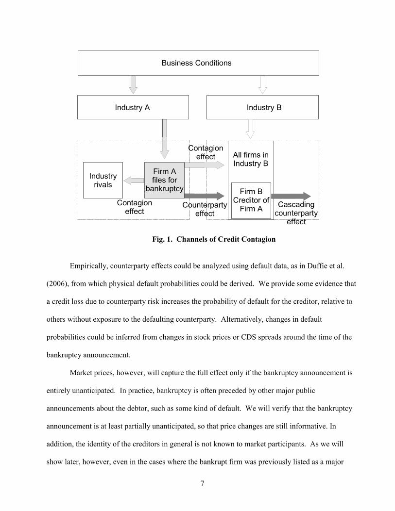
Figure 1 describes channels of credit contagion. When Firm A defaults, or files for

bankruptcy, we generally expect negative effects for other firms in the same industry. Contagion

effects reflect negative common shocks to the prospects of the industry, and may lead to further

failures in industry A. On the other hand, the failure of a firm could help its competitors gain

market share. Generally, however, the net of these two effects is intra-industry contagion.

Contagion effects can also arise across industries. Suppose that Industry A is a major client of

Industry B. The default of Firm A could then reveal negative information about sales prospects for

firms in Industry B.

Another channel, however, is the direct counterparty effect. Say that Firm B has made a

trade credit, or loan to Firm A. Default by Firm A would cause a direct loss to Firm B, possibly

leading to financial distress. This could cause cascading effects to creditors of Firm B. This paper

focuses on the counterparty effects between Firms A and B, measuring the price impact for Firm B

while controlling for price effects for all firms in the same industry.

Generally, cascading or looping effects are too complex to model analytically because firms

may hold each other’s debt and also because of the sheer number of networked firms.10 Jarrow and

Yu (2001), for example, do provide closed-form solutions but only for a simple case with two firms

and no cascading effects.

10 The case where firms hold each other’s debt more properly describes a banking network. Several papers, summarized for instance in Upper (2007) analyze contagion effects via simulations. One problem, however, is that bilateral exposures are generally not available.

7

Business Conditions

Industry A

Firm A files for

bankruptcyIndustry

rivals

Industry B

Firm B Creditor of

Firm A

Contagion effect

All firms in Industry B

Contagion effect

Counterparty effect

Cascading counterparty

effect

Fig. 1. Channels of Credit Contagion

Empirically, counterparty effects could be analyzed using default data, as in Duffie et al.

(2006), from which physical default probabilities could be derived. We provide some evidence that

a credit loss due to counterparty risk increases the probability of default for the creditor, relative to

others without exposure to the defaulting counterparty. Alternatively, changes in default

probabilities could be inferred from changes in stock prices or CDS spreads around the time of the

bankruptcy announcement.

Market prices, however, will capture the full effect only if the bankruptcy announcement is

entirely unanticipated. In practice, bankruptcy is often preceded by other major public

announcements about the debtor, such as some kind of default. We will verify that the bankruptcy

announcement is at least partially unanticipated, so that price changes are still informative. In

addition, the identity of the creditors in general is not known to market participants. As we will

show later, however, even in the cases where the bankrupt firm was previously listed as a major

8

customer in the creditor’s annual report, creditors suffer a very large price drop upon the bankruptcy

announcement.

We expect that the announcement of bankruptcy by Firm A will lead to lower stock prices

and wider CDS spreads for creditor firms. To abstract from more general contagion effects, or

perhaps cascading effects in Industry B, the analysis controls for average price effects in Industry B.

For example, financial distress in the U.S. automobile industry had negative effects on the parts

supplier industry. Among part suppliers, however, those with direct credit relationships have

suffered more than others. Adjusting for the industry effect should provide cleaner estimates of the

direct counterparty effect.

The analysis can be further enriched by cross-sectional information. The stock price effect

for Firm B can be decomposed as follows. Define: AMOUNT as the dollar amount of unsecured

credit exposure, MVE as the market value of the creditor’s equity prior to the announcement, EXP

as the scaled or relative exposure, measured as AMOUNT divided by MVE, REC as the fractional

recovery rate, and NPV as the dollar amount of losses of future profits from the customer-lender

relationship, also scaled by MVE.

In the simple 2-firm model, the direct wealth effect of a debtor’s bankruptcy can be

measured by the change in the creditor’s stock price, which requires dollar amounts to be scaled by

the market value of equity. Thus, the rate of return can be conceptually decomposed into:

RATE OF RETURN EXP(1 REC) NPV= − − − (1)

which involves an immediate default loss, i.e., the exposure times one minus the recovery rate, plus

an effect expressed as the net present value of lost future business. More generally, cascading

effects can also arise. Note that Equation (1) does abstract from frailty effects when the rate of

return is adjusted for that of other firms in the same industry.

9

For trade credit, the NPV term could be quite large, reflecting the loss of an on-going

business relationship with a major customer. For bond investors, this NPV term should be zero

because there is no other business flow between the investor and the debtor. For banks, the NPV

term should be small if the value of the banking relationship with the client represents a small

fraction of profits. We will verify whether counterparty risk is stronger for industrial creditors than

financial creditors, holding exposure constant.

Our paper is related to Dahiya et al. (2003), who examine the costs and benefits of banking

relationships over the period from 1987 to 1996.11 They find a significant negative wealth effect for

the shareholders of the lead lending banks on the announcement of bankruptcy and default by

borrowers. Ours differ from theirs in several important ways. First, they focus on the leading bank

in the case of loans, while we examine all major creditors, including financial institutions such as

insurance companies, as well as industrial corporations. Second, the only form of credit in their

study consists of loans, which are usually senior and secured. Our study includes unsecured loans,

bonds, and trade credit, which is a greater variety of debt types. In addition, unsecured debt is more

likely to induce contagion effects due to the lower recovery rates on unsecured debt. We also

follow the creditor through time, and assess the effect of the initial bankruptcy on the subsequent

default probability.

II. Data and Descriptive Statistics

A. Identification of Creditors

We collected information on 721 Chapter 11 bankruptcies that occurred between January

1999 and December 2005. The information was retrieved from the website

11 Another paper by Kracaw and Zenner (1996) examine bank share price reactions to nine highly leveraged firms that became financially distressed. They find a negative share price reaction for these banks, but one that was not statistically significant. However these findings were for a very small sample of firms involved in highly leveraged transactions such as LBOs or recapitalizations.

10

www.bankruptcydata.com and includes information on the top twenty unsecured claimholders, i.e.,

creditor names, credit types, and credit amounts extended to the bankrupt firm. The identity of the

creditors is generally not available from public filings.

For example, Enron filed for bankruptcy on December 2, 2001. With $63.3 billion in assets,

this was the second largest bankruptcy in history. In accordance with Federal Regulation

bankruptcy 1007(d) for filing under Chapter 11, the petition included the top twenty unsecured

creditors. Citibank was the largest unsecured creditor, with $1.75 billion in claims. The following

week, the bank announced a write-down of $228 million related to unsecured Enron positions.12

Citibank had not mentioned its exposures to Enron in annual reports before 2001.

We then excluded all claims by individuals as well as claims from local, state, and federal

governments, and other non-profit organizations.13 Bankruptcies must have at least one remaining

creditor. This reduced the sample to 351 bankruptcy events, with 4796 event-creditors. We also

eliminated all bond debt reported by a commercial bank, investment bank, broker/dealer, and asset

manager, because these institutions generally serve as trustees for the bond investors and do not

bear the credit loss.14

For the purpose of the subsequent analysis, we require creditors to have equity returns

available from CRSP. As we also require firm characteristics, we match identifying codes in CRSP

and COMPUSTAT for both bankrupt firms and creditors.15 To avoid a potential contamination

issue, we check the [−5, +5] event window around the bankruptcy filing in the ABI/Inform database

to make sure that creditors have no other informative corporate news of their own. This is the

longest window centered on the event that is used later in the empirical analysis. 12 Source: ‘Citigroup Posts 36% Rise in Earnings’, by Paul Beckett. Wall Street Journal, Jan 18, 2002, page, A-3. 13 Most of individual claims arise from employment contracts, bonuses, compensations, etc. Local or state government claims usually represent taxes. 14 For instance, the largest single claim in our original sample is listed as a bond claim worth $17.2 billion to WorldCom held by JP Morgan Chase. In its annual report, however, the bank does not even mention direct exposure to WorldCom. Losses were borne by bondholders. So, this observation is discarded from the sample, as are all similar ones. 15 For firms with a name close to the COMPUSTAT company name, we use an algorithm to look for its 6-digit CNUM code in COMPUSTAT and Permanent number in CRSP. If this method fails, we hand collect the code.

11

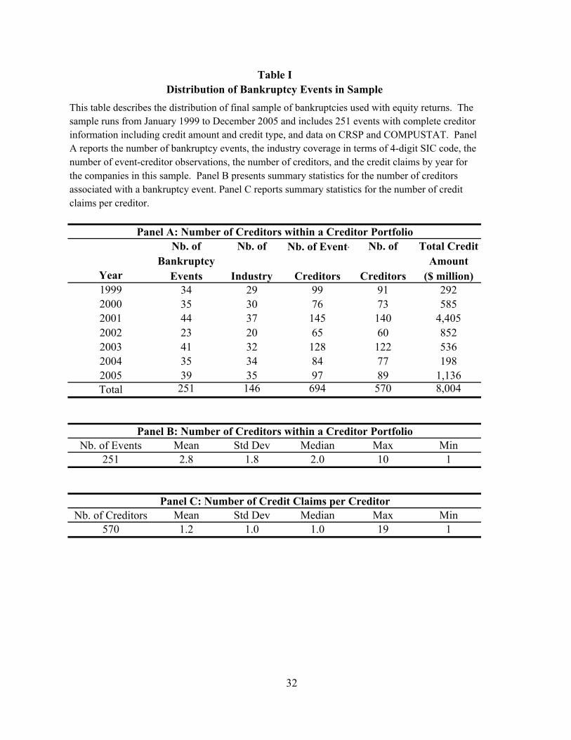
Table I shows the final sample for equity returns. Panel A describes the distribution of

bankruptcy filings, industry coverage, number of event-creditors, number of creditors, and credit

amounts by year. The sample consists of 251 bankruptcies, 146 industries, 694 event-creditor

observations, and 570 creditors. The borrowers and creditors are generally in different industries;

only 40 creditors out of 570 are in the same industry as the borrower. The aggregate claims add up

to $8 billion for the creditors in this sample.

[Insert Table I]

Panel B shows that the number of public creditors ranges from 1 to 10, with a mean of 2.8

and median of 2. As shown in Panel C, the median creditor has only one exposure to the 251

bankruptcy events. Some companies have much more exposure, however. The largest number of

claims is 19, indicating that this creditor, the commercial bank JP Morgan Chase, is involved in 19

bankruptcies where it is in the top creditor group.

This paper also uses CDS spreads taken from a comprehensive dataset from the Markit

Group. The original dataset provides daily quotes on CDS spreads for over 1,000 North American

obligors from January 2001 to December 2005. Quotes are collected from a large sample of banks

and aggregated into a composite number, ensuring reasonably continuous and accurate price

quotations.16 We use the five-year spreads because these contracts are the most liquid and

constitute over 85% of the entire CDS market. To maintain uniformity in contracts, we only keep

CDS quotations for senior unsecured debt with a modified restructuring clause and denominated in

U.S. dollars. Because there are fewer CDS quotes than stock price quotes, the CDS sample is

smaller than the equity sample. The CDS final sample consists of 128 bankruptcies, 209 event-

creditor observations, 178 creditors, and 91 industries.

16 The Markit Group collects more than a million CDS quotes contributed by more than 30 banks on a daily basis. The quotes are subject to filtering that removes outliers and stale observations. Markit then computes a daily composite spread only if it has more than three contributors. Once Markit starts pricing a credit, it will have pricing data generally on a continuous basis, although there may be missing observations in the data. Because of these features, the database is ideal for time-series analysis. These data have also been used by Micu et al. (2004) and Zhu (2006).

12

B. Description of Credit Claims

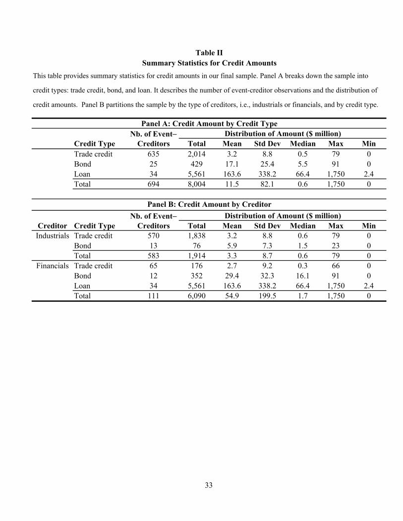
Table II breaks down credit claims by credit type and creditor type. Panel A partitions

claims into three major credit types: trade credit, bond, and loan. The trade credit category accounts

for a large fraction of the number of events. There are few cases of unsecured loan claims, due to

the fact that most bank loans are secured. The average size of the claim differs widely across credit

type. For trade credit, the average claim is $3.2 million, which seems small. For bonds, this is

$17.1 million. Loans have the largest average exposure, at $163.6 million.

[Insert Table II]

Next, Panel B partitions the sample by type of creditors. Firms with industry SIC code

falling between 6000 and 6999 are classified as financial institutions. These include commercial

banks, savings institutions, securities brokers and dealers, insurance companies, credit-card

companies, real estate investment trusts, and other financial services. The rest are grouped as

industrial firms. We have a total of 583 event-creditors for industrial firms. As expected, trade

credit is the main credit type for industrial creditors, accounting for 98% of 583 cases. The single

largest trade credit is $79 million due to NEC Corporation and recorded when ICO Global

Communications Holdings, a satellite firm, filed for bankruptcy in 1999.

For financials, we have 111 event-creditors. Loans are the most important credit types.17

The single largest exposure is an unsecured loan of $1.75 billion due to Citibank by Enron in 2001.

The average credit amount for financials is $54.9 million, which is much larger than the average

exposure of $3.3 million for industrials.

17 In this sample, all loans are made by commercial banks.

13

Finally, we obtain recovery rates from Fitch (2005), which reports historical recovery rates

of senior unsecured bonds for 24 industries over the period 2000 to 2004.18 We use average

recovery rates by industry. In practice, however, actual recovery rates vary by name, industry, and

even over time. So, this is an approximation. In addition, these recovery rates are estimated from a

bond sample, and may not fully reflect recovery rates for trade credit or bank loans.19

III. Method

This paper investigates the market reaction of creditors around bankruptcies. For each

event, we construct a creditor portfolio as an equally-weighted portfolio of firms. On average, there

are 2.8 firms in the creditor portfolio. Using equally-weighted portfolio matches the method used

for the construction of CDS indices; similar results, however, hold using value-weighted portfolios.

We then apply the standard event study method. First, we calculate abnormal returns (ARjt)

for firm j at time t using the market model methodology following MacKinlay (1997), with

parameters estimated over a window ranging from 252 days before the event date to 50 days before

the event date. Next, these abnormal returns are averaged across bankruptcy events for creditor

portfolios. Cumulative abnormal returns (CAR) are then computed from time t1 to t2. Finally, t-

statistics are computed from the portfolio time-series standard deviation to account for any possible

event clustering.

The stock price response of the creditor can be attributed to two types of effects. The first is

a direct counterparty effect, due to the immediate loss from default, and is specific to the creditor.

The second is a contagion or cascading effect spreading to the rest of the industry. To isolate the

first effect, the market model is estimated for each firm relative to two portfolios. The first is the

18 Recovery values are computed from the price of defaulted securities one month after default and are par-weighted averaged. The mean of average recovery rates is 33% across industries, with a low of 12% for insurance and 66% for gaming, lodging, and restaurants. 19 Moody’s (1999) reports that the average recovery rate on trade claims is 74%, which is higher than the 70% rate for senior unsecured obligations, although the sample size is small.

14

market index, proxied by CRSP’s value-weighted index for NYSE/AMEX/Nasdaq stocks. The

second is a portfolio of firms in the same industry as the creditor. This industry index is constructed

as a portfolio of value-weighed industry equity returns for all firms with the same three-digit SIC

code.

For CDS spreads, we also report measures that are adjusted for general market conditions, as

proxied by the same credit rating category, to obtain the rating-adjusted CDS spread (AS). For firm

j with rating r at time t, jtAS is defined as jt jt rtAS S I= − , where jtS denotes the CDS spread of

reference entity j at day t, and rtI denotes that of the investment-grade or high-yield CDS index at

day t, depending on whether the rating r falls into the investment-grade or the high-yield grade

category. We use the actual spread levels for the Investment Grade CDX (CDX.NA.IG) and the

High Yield CDX (CDX.NA.HY) to represent these two CDS indices since their inception in April

2004. We extend the indices backwards to January 2001 following the CDX index construction

methodology.20 The Investment Grade CDX is an equal-weighted index made up of 125 firms with

the most liquid investment-grade credits. The High Yield CDX is an equal-weighted daily index

composed of 100 high-yield entities. Both indices cover companies domiciled in North America.

For each event, cumulative abnormal CDS spread changes (CASCs) are calculated as

2 11 2( , )j jt jtCASC t t AS AS= − , and then processed as in the case of equity returns.

IV. Empirical Results A. Market Reaction for Bankrupt Firms

Before we examine the effect of financial distress on the creditor’s equity returns, we first

measure the effect of distress on the borrower itself. To the extent that the bankruptcy

announcement is unanticipated, we expect the borrower’s stock price should experience significant 20 The methodology can be found at the website: http://www.markit.com/information/affiliations/cdx.html. The list of component companies as of April 2004 was used to backfill the series.

15

negative abnormal returns upon the bankruptcy filing. Since many companies had been delisted

before the bankruptcy event, the number of borrowers for which these returns are available is

considerably smaller than the size of the creditor sample.

We find an average announcement day abnormal return of –16.6% for 66 firms that file for

bankruptcy. This is economically and statistically significant. Over a 3-day period, the cumulative

abnormal return amounts to -30.0%. These results are comparable to the 2-day loss of -21%

reported by Lang and Stulz (1992) and indicate that bankruptcy announcements are not fully

anticipated by the market, justifying the use of market data in the analysis.

B. Market Reactions for Creditors

Even if a firm’s bankruptcy is not totally unexpected, the announcement also reveals the

identity of creditors and the size of their exposures. This brings new information to markets and

allows us to quantify the effect of counterparty risk, net of industry effects. The principal results are

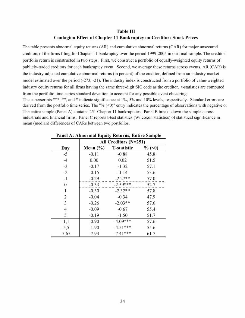
presented in Table III. Panel A reports abnormal returns for the creditor portfolio using the entire

sample of 251 events. The average CAR for the portfolio is negative, at −0.90% (t = −4.09) for the

3-day event window and −1.90% (t = −4.51) for the 11-day event window. The fraction of firms

with negative returns is greater than 50 percent, indicating that these averages are not skewed by

just a few observations. Thus, there is a significant negative wealth effect on a creditor’ equity

when a borrower files for Chapter 11 bankruptcy protection, as expected. Note that the magnitude

of this effect is greater than the intra-industry contagion observed for industry peers. Jorion and

Zhang (2007) report an 11-day return of −0.41% for firms in the same industry as the bankrupt

company. The effect here is four times greater. The total effect of -1.90% does not seem very

large in absolute terms, but the average exposure is only about 0.30% of the market value of equity,

as will be seen later. Thus the wealth effect is much bigger than the immediate credit loss.

[Insert Table III]

16

We then examine whether this effect differs across industrial or financial creditors, by

constructing two creditor portfolios for each event, one containing industrial creditors, and the other

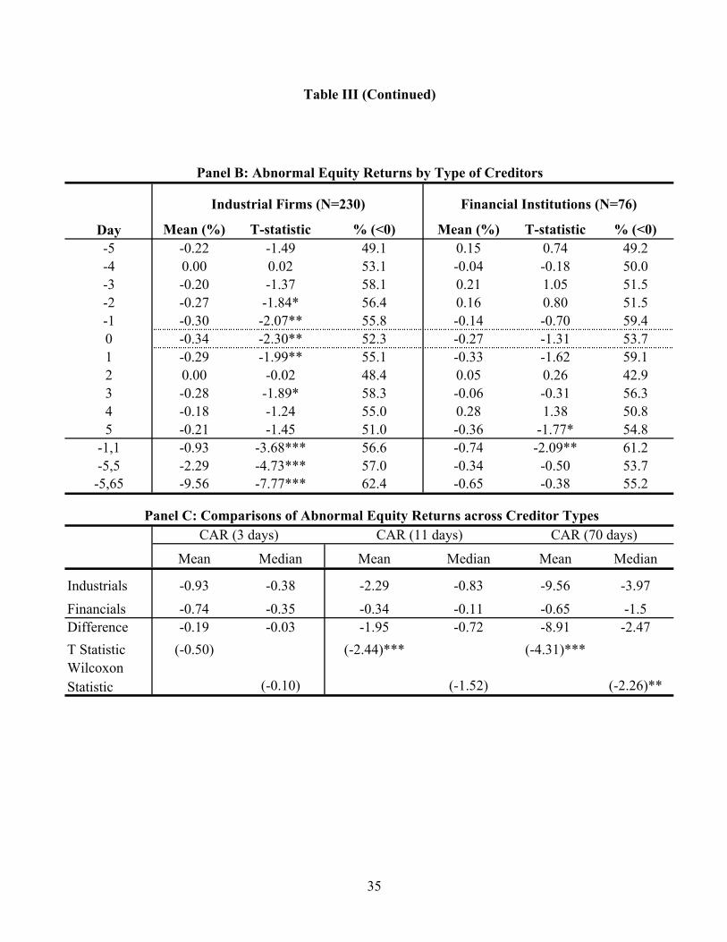
containing financial institutional creditors. Results are presented in Panel B of Table III. For

industrial creditors, the average CARs is −2.29% for the 11-day window. Furthermore, the

negative price impact persists over longer windows.

For financial institutional creditors, the average CARs is −0.34% for the 11-day window.

The effect is much less than for industrials and not statistically significant. Dahiya et al. (2003)

report slightly stronger effects, with 5-day returns of −0.91% for the lead banks exposed to

bankruptcy events, over a different sample period.

As previously noted, Table III reports abnormal returns adjusting for industry effects, which

represent pure counterparty risk. We also performed the analysis adjusting for the overall market

rather than the creditor’s industry. Results are similar and are not presented here.

Panel C reports test statistics of differences across groups, which are statistically significant

for the 11-day and 70-day windows. Therefore, financial institutions are less affected by

counterparty credit losses than industrials, conditional on being in the list of top creditors.

Potentially, this could be explained by a smaller exposure relative to their assets. To further

understand the drivers of this effect, we need to turn to cross-sectional regressions.

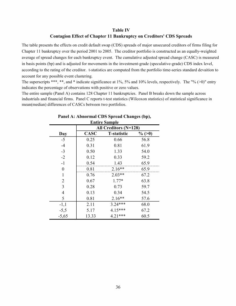
Next, Table IV reports effects on creditor’s CDS spreads.21 For the entire sample, the

average CDS spread, adjusted for the ratings, increases by 2.11 basis points (bp) for the 3-day

window and by 5.17 bp for the 11-day window. Both numbers are significant, and confirm the

information from equities. This 5bp spread increase can be compared to the level of CDS spreads

for different credit ratings. Over the 2001-2006 period, the median spread was 30bp for A credits,

37bp for A−, 46bp for BBB+, 59bp for BBB, and 87bp for BBB−. Thus the 5bp increase in spreads 21 We also calibrated the Jarrow and Yu (2001) (JY) model to the term structure of CDS spread for creditors before and after the bankruptcy event. Due to its simplifying assumptions, however, the model is unable to reproduce the actual change in CDS spreads.

17

corresponds roughly to a drop in credit rating from A to A−, or to less than half of the difference

between BBB+ and BBB spreads. Further, to the extent that the bankruptcy is anticipated, the

increase in default probability should be even higher. Later, we will see that this signal indeed

translates into a higher failure rate for the creditor.

[Insert Table IV]

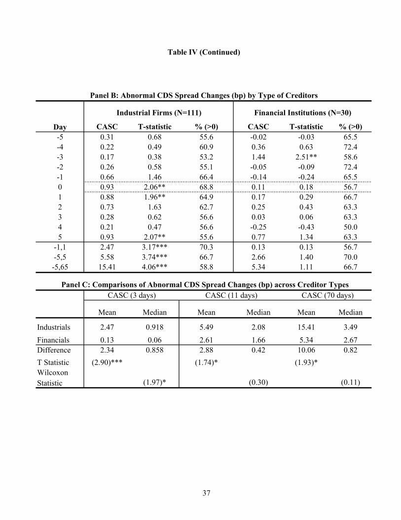
Panel B splits the sample into industrials and financials. For the first group, the 11-day

effect is an increase of 5.58bp, versus 2.66bp for the second group. These numbers confirm the

findings from equity prices that industrials are much more affected by this credit loss than

financials. Here, the difference is statistically significant across the 3-day, 11-day, and 70-day

windows.

C. Cross-Sectional Reactions

This section examines to what extent counterparty effects are related to creditor

characteristics. This is useful to understand the drivers of counterparty risk. To this end, we

estimate cross-sectional regressions where the dependent variable is the 3-day industry-adjusted

CAR around the event date. The most general specification is:

*1 2 1 3 4 5CAR EXP REC EXP(1-REC) CORR VOL LEVα β β β β β β ε= + + + + + + + (2)

where EXP is the exposure ratio, or ratio of credit amount to the total market value of the creditor’s

equity, REC is the recovery rate for firms in the same industry as the bankrupt firm, CORR is the

correlation of equity returns between the creditor and the borrower for 252 days preceding the

event, VOL is the equity return volatility of the creditor for the year preceding the bankruptcy, and

LEV is the average of leverage ratio of the creditor over the previous four quarters, defined as the

ratio of book value of debt over the market value of assets, taken as the market value of equity plus

the book value of debt.

18

In what follows, we give the predicted sign of the coefficient for the equity regressions. For

the CDS spread regressions, all signs should be inverted.

A creditor with greater exposure to the distressed firm is more likely to be hurt from the

bankruptcy, so we hypothesize the coefficient on EXP to be negative. For industries with a greater

recovery rate, the expected credit loss should be less, and the price impact more muted. We

hypothesize a positive coefficient for REC.

In our specifications, we also use the variable EXP(1-REC), which is the expected credit

loss upon default. If default was totally unexpected and these variables measured without error, we

should find a coefficient of −1 on this variable for the regression on equity returns. In practice,

these conditions are not totally satisfied, which should bias the coefficient toward zero. However,

Section I argued that a business loss effect may also arise. Assuming this is proportional to the

expected credit loss, this should increase the size of the slope coefficient, taken in absolute value.

The observed coefficient should reflect the net of these two effects.

We also include CORR as an additional variable, to control for previously observed

correlation between the creditor and debtor. Contagion effects are expected to be greater for

creditors with higher equity correlation with the borrower, due to commonality in cash flows. As a

result, the coefficient on CORR is expected to be negative.

We also add variables that proxy for the creditor’s future default probability. Merton-type

structural model suggests that companies with higher equity return volatility and higher leverage are

associated with a higher default probability. We expect such firms are more vulnerable to negative

shock from their borrowers, implying negative coefficients for LEV and VOL. Also included in the

regression is a set of year dummies and industry dummies based on the one digit SIC code of the

borrower.

19

We also examined the extent to which credit derivatives use by commercial banks can affect

exposure. Only seven banks in our sample have such information, however, and the results were not

significant.

Summary statistics for the main variables are presented in Table V. Several points are

noteworthy. The average size of bankrupt firms is $1.9 billion in terms of assets. This is much

smaller than the average size of creditors, which is $97.9 billion. The average credit amount is

$11.5 million only, from Table II. This explains why the average exposure is fairly small, at 0.32%

of creditor equity. Average recovery rates are around 0.30. The average rating of creditors is 9.3,

which is close to BBB.

There are differences across industrials and financials, however. Table II has shown that the

average credit exposure for industrial creditors is $3.3 million, much smaller than the average of

$54.9 million for financials. However, taking into account the fact that industrial creditors are

much smaller than financial creditors, the average credit exposure is 0.32% for industrial creditors,

against 0.16% for financial institutions.

[Insert Table V]

Table VI presents the results of the cross-sectional regressions. OLS regressions are

estimated separately for the entire sample, for industrials, and for financials. While the slope

estimates are consistent, standard errors should account for the fact than many of these CARs are

measured over the same period, for each bankruptcy event. As a result, we report t-statistics based

on clustered standard errors, which are adjusted for event clustering.

[Insert Table VI]

As predicted, the coefficients on EXP are negative and statistically significant. We also

find that the coefficients on REC are positive, as expected, but barely significant for the overall

20

sample, perhaps because there is not enough meaningful variation within this sample, or because of

measurement error.22

Model 3 uses the expected credit loss, EXP(1-REC), conditional on default. For the entire

sample, the coefficient is −1.01, which is significantly different from zero but not from one. The

size of the coefficient is particularly interesting. A coefficient of −1 would indicate that, when a

creditor unexpectedly defaults, an exposure of 1% of equity market value is associated with a

wealth loss of 1%. This number can differ from −1 for two reasons. First, if the bankruptcy

announcement is not totally unexpected or if the variables have measurement errors, the slope

should be biased toward zero. Second, if the bankruptcy implies a loss of future business, the slope

should be even lower than −1. The actual coefficient should reflect the net of these two effects.

For industrials, the coefficient on EXP(1-REC) is −0.996. For financials, this coefficient is

−2.09. Both coefficients are significantly different from zero but not from one. The size of the

latter number is somewhat puzzling. This could be due to the use of 3-day equity abnormal returns,

which were similar for the industrial and financial subsamples, but much more different over longer

intervals and for the CDS data. A possible explanation for this large number is that the loss due to

bankruptcy may induce investors to reconsider the risk of the entire bank portfolio, as in the

learning hypothesis advanced by Collin-Dufresne et al. (2003). An alternative explanation for the

high coefficient for financials is that there could be some additional unrecorded exposure. For

example, financial letters of credit or similar off-balance sheet items create bank commitments that

are exercised by a third party if the underlying credit fails. Alternatively, the recovery rate could be

underestimated for banks either because they choose loans that are more likely to have higher

recoveries, or because they take a more active part in the resolution of the bankruptcy process.

22 Dahiya et al. (2003) find that a recession dummy (July 1990-March 1991) is significant, which can be interpreted as an indicator of lower recovery rates during recessions. If so, assuming fixed recovery rates will induce measurement errors.

21

Next, the CORR coefficients are negative and significant for the entire sample and the

industrial sub-sample, as expected. Including this coefficient does not affect much the coefficients

on expected credit loss, however. The latter are slightly lower, but still significant. Consistent with

our hypothesis, the coefficients on VOL are negative, and generally significant. The coefficients on

the LEV variable are all negative but insignificant.

Table VII repeats the cross-sectional regressions for CDS spread changes. The coefficients

have systematically opposite signs to those in Table VII. As predicted, changes in spreads are

positively related to exposure, negatively to recovery rates, positively to prior equity correlation,

equity volatility, and leverage. The slope coefficient on exposure is around 8, indicating that a

credit exposure of 1% is associated with an increase of 8bp in the credit spread over the 3-day

interval. Given that the average exposure is only 0.3% in this sample, this explains the small

increase of 2bp only reported in Table IV over these 3 days.

Here, industrials are more affected by credit events than financials. The coefficient on the

expected credit loss, EXP(1-REC), is 17.08 as compared to 7.65 for financials. The results for this

sample conform better to our expectations.

[Insert Table VII]

D. Discussion and Additional Evidence

Counterparty risk should be greater under a number of conditions. Creditors must have a

substantial portion of their economic value tied up with the bankrupt firm. In addition, the recovery

rate must be low, and the bankrupt firm must shrink sufficiently to affect future business

opportunities. For cascading effects to be important, the bankrupt firm must be large as well. We

provide additional evidence on these conditions.23

Market losses for industrials are generally greater than the direct default losses, which

suggests that price changes also account for the net present value of lost future business. Such 23 This section substantially benefited from the referee’s comments.

22

losses may not always materialize, however, especially when companies continue to operate under

the protection of Chapter 11 bankruptcy code. On the other hand, the NPV term is more likely to be

substantial when the bankrupt firm liquidates. As an additional check, we construct a subsample of

bankrupt firms that were likely to be liquidated.24 The average 3-day CAR for creditors is -1.32%,

with a t-statistic of -2.66, which is greater in absolute value that the CAR in Table III. In addition,

the cross-sectional regression coefficient on EXP(1-REC) in Model 3 changes from −1.01 to −2.26.

These additional results confirm our hypothesis. The price reaction when the debtor liquidates is

stronger than when it reorganizes because the creditor will incur a loss not only on its exposure, but

also from its future business.

Overall, however, market losses due to counterparty default on average are small for this

sample. This is because the average exposure is small, at 0.32% of equity only. Using Model 3 in

Panel A of Table VI, this translates into a fitted loss of −1.01, close to the average loss of −0.90

reported in Table III. This market loss, however, should be much greater for larger exposures.

From Table V, the maximum exposure is 37.3%, which translates into a fitted loss of −27.2%. This

appears serious enough to cause financial distress for the creditor.

Alternatively, we also examine a subsample of creditor firms for whom the bankrupt firm

represents a large fraction of sales. Firms have to disclose in their 10-Ks the identity of any

customer representing more than 10% of total sales. For this sample, we find six cases where the

creditor lists a firm subsequently filing for bankruptcy as a major customer in the previous two

fiscal years. The average exposure ratio is 11.11% for this group. Around the bankruptcy

announcement, we find that the average 3-day, 11-day, and 70-day industry-adjusted CARs are

−9.23% (t=−2.10), −23.34% (t=−2.99), and −53.17% (t=−2.91), respectively. Around the default

24We searched the bankruptcy announcement for terms such as “use Chapter 11 as a vehicle to facilitate its liquidation”, “orderly liquidation of the company’s assets”, “wind down operations”, “for a sale of substantially all of the assets”, and so on. This gave a subsample of 32 events with 79 creditors.

23

date, the average 3-day, 11-day, and 70-day industry-adjusted CARs are −12.19% (t=−2.42),

−18.71% (t=−2.89), and −51.21% (t=−3.06), respectively. Thus, for firms with large exposures,

counterparty default creates substantial market losses, which are a harbinger of subsequent financial

distress.

E. Subsequent Financial Distress

We now examine the effect of the bankruptcy on our creditor sample. Counterparty risk

arises if a credit loss increases the probability of default of the creditor, compared to others. Table

VIII follows the creditors through time, examining the fraction of firms that are delisted or

downgraded within one and two years.

[Insert Table VIII]

First, examine the group of 461 industrial creditors with a credit rating. Of these, 9

companies are delisted due to distress within one year, and 12 are delisted within two years.25 This

represents 1.95% and 2.60% of the sample, respectively. To test whether these numbers are

abnormally high, we construct a control sample for each creditor that consists of all firms in the

same industry, with the same credit rating, and in the same size group, using a partition around the

median of total assets. The fraction of firms that are delisted in this control sample within one year

and two years is 0.28% and 0.56%, respectively. Therefore, the control sample has a much lower

fraction of firms experiencing a delisting. The table reports tests of equal fractions, which show

that differences are significant at the 1% level. The difference between the two samples is also

economically important. For instance, an increase in the annual default rate from 0.28% to 1.95% is

equivalent to pushing a BBB rated borrower into the BB− category.

25 In this section, the delisting information is obtained from CRSP. We confine our attention to delisting due to financial distress. This corresponds to delisting code starting with 4 and 5.

24

The table also compares the fraction of firms downgraded within one and two years of the

events for the creditor sample and the control sample. The difference is striking. Within one year,

the fraction of downgraded firms is 23.64% for industrial creditors and 8.33% for the control

sample. The difference is statistically significant at the 1% level. Thus, the probability of a

downgrade of a company suffering a credit loss is about three times the unconditional probability.

For the sample of 100 financial creditors with a credit rating, only one company was delisted

within the following one or two years. Thus the counterparty effect on financials is minor in this

sample. We observe, however, that 14% and 20% of these companies experienced a downgrade in

the ensuing one and two years. These fractions are twice those in the control sample, with both

differences significant at the 1% level. Financial creditors that suffer a credit loss are more likely to

experience downgrades later.

Even so, financial distress is more acute for industrials, where a greater fraction of firms are

delisted or downgraded later. This largely confirms the evidence in Table IV that 11-day CDS

spreads increase by 5.58bp for industrials, against 2.66bp for financials.

The comparison with the control sample indicates that credit losses are associated with

significantly greater financial distress for the creditor. This evidence is indirect, however. We also

searched multiple databases for news stories for the 13 delisting and 169 downgrade cases. Among

the 13 delisting cases, one news story explicitly linked the delisting to the previous bankruptcy.

Among the 169 downgrade cases, there are 8 cases indicating that the creditor was severely affected

by the prior bankruptcy, 25 cases where the creditor-debtor relationship was explicitly mentioned,

53 cases where it was pointed out that the creditor and debtor are in the same industry, and 83 cases

with no news. We would not expect full coverage of downgrades for small companies, however.

Thus, there is some direct evidence of contagion from news reports, but it is limited.

25

V. Implications for Portfolio Risk

The economic importance of these results is now investigated using simulations calibrated to

the empirical findings in this paper. Take a homogeneous sample of N=100 companies, all with

unconditional probability of default (PD) of 1% over one year. This number represents the average

default rate of BB rated firms. The goal of this analysis is to derive the distribution of number of

defaults in this portfolio, using first a conventional factor model and then introducing counterparty

risk. The question is whether counterparty risk can explain the greater clustering of defaults

observed in practice.

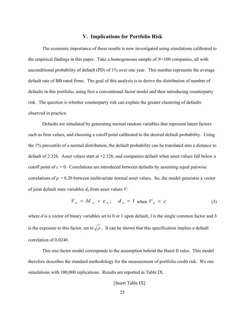
Defaults are simulated by generating normal random variables that represent latent factors

such as firm values, and choosing a cutoff point calibrated to the desired default probability. Using

the 1% percentile of a normal distribution, the default probability can be translated into a distance to

default of 2.326. Asset values start at +2.326, and companies default when asset values fall below a

cutoff point of c = 0. Correlations are introduced between defaults by assuming equal pairwise

correlations of ρ = 0.20 between multivariate normal asset values. So, the model generates a vector

of joint default state variables dit from asset values V:

1; =+= itititit dbIV ε when cV it < (3)

where d is a vector of binary variables set to 0 or 1 upon default, I is the single common factor and b

is the exposure to this factor, set to ρ . It can be shown that this specification implies a default

correlation of 0.0240.

This one-factor model corresponds to the assumption behind the Basel II rules. This model

therefore describes the standard methodology for the measurement of portfolio credit risk. We run

simulations with 100,000 replications. Results are reported in Table IX.

[Insert Table IX]

26

The first column describes simulation results for the standard model. Initially, there is no

counterparty risk. The replications produces an average default rate dt across the 100 obligors. In

the first column, the average default rate across all replications is 1.00%, which is in line with the

underlying PD of 1%. The default correlation is estimated at 0.0237, which is very close to the

theoretical value of 0.0240.26 The table also shows the percentiles of the distribution. For example,

the 99.99% quantile, which is often used as a measure of economic capital by commercial banks,

has 23 defaults. In other words, there is only a probability of 0.01% or less that 23 firms or more

out of 100 will default over the next year based on this model. This type of information is routinely

used to create tranches on a portfolio of debt obligations.

The next step is to introduce counterparty default. In Table I, the mean number of creditors

was 2.8, so we initially assume that each company has N=3 counterparties only. When the borrower

goes into default, the creditor’s default probability is increased. Table IV shows an increase in CDS

spread of 5bp over a 11-day window. Assuming a recovery rate of 30%, this implies an increase in

the risk-neutral default probability of 5/0.30, or 0.17% for the creditor. The actual increase in PD is

probably higher because this is the purely unanticipated component. Table VIII show a much

higher increase in actual PD for the affected creditors. So, we start with an increase in default

probability of 0.50%. This shock is represented by an immediate fall in the asset value. Increasing

the unconditional PD from 1.00% to 1.50% changes the normal deviate from 2.326 to 2.170, which

represents a fall of k = −0.156.

The model for asset values V with counterparty risk is described in Equation (4). The

second term now represents counterparty risk, with the vector of defaults d affecting V through a

matrix A. Without loss of generality, firms are sorted by counterparty exposure. For example,

firms 2, 3, and 4 have exposure to obligor 1, and so on. Thus, the first column in A has zeroes

26 The default correlation is estimated from the variation in the average default rate across replications, as explained in De Servigny and Renault (2004).

27

except for the entries two to four, which are set to 1. Upon default by the first company, the asset

values for firms 2, 3, and 4 are immediately decreased by k, which may cause default for any of

these three companies. In turn, this may precipitate other defaults. If so, this process can be

iterated up to the point where the number of defaults stabilizes.

it t t itV bI kAd ε= + + (4)

This framework allows us to model the effect of cascading defaults. Consider, for example,

the first column under “Counterparty Risk” in Table IX, with N=3 and conditional PD of 1.50%.

Without counterparty risk, the default correlation is 0.0237. With the first counterparty default, this

increases from 0.0237 to 0.0278. With multiple defaults, this increases further to 0.0291. This

increase in default correlation can be translated back into a higher asset correlation for the baseline

model, Equation (3). Here, we would need to have an increase from 0.200 to 0.226, which is

substantial. Indeed Das et al. (2007) report that, even after fitting a time-varying intensity model

for U.S. corporate defaults, there is still substantial clustering of defaults. They calibrate a normal

copula to the residuals and find an excess correlation ranging from 0.01 to 0.04. The increase of

0.226-0.200=0.026 reported here falls within this range. Thus, counterparty risk provides a

potential resolution to the observed excess clustering of defaults.

These counterparty effects have important implications for the shape of the default

distribution. The table shows that the 99.99% percentile has increased from 23 to 29 defaults when

counterparty effects are included and N=3. Relying on the baseline model would underestimate the

number of defaults that could occur in a bad scenario.27 Thus, ignoring this credit contagion effect

implies that the likelihood of large losses would be underestimated.

27 When counterparty effects are added, the average default rate goes up slightly, from 1.00% to 1.05%. So, strictly speaking, the results with counterparty risk should be compared to the standard model with no counterparty risk and PD=1.05%. The second column, however, shows that this increase in the PD has no effect on the tails in the usual factor model.

28

The rest of the table explores the effect of alternative parameters. The default distribution

has longer tails when the conditional probability increases. For instance, going from 1.50% to

2.00% increases the 99.99% percentile from 29 to 35. Similarly, the tails extend when the number

of counterparties increases. For instance, going from N=3 to N=10 increases the 99.99% percentile

from 29 to 65. This will substantially increase the default probability of the senior tranche.

Consider for example a portfolio structured to ensure an AAA rating for the senior tranche.

Without counterparty risk, this requires the junior tranche to absorb the first 23 defaults. With

counterparty risk and N=10, however, the senior tranche effectively has the default probability of a

BBB bond.28

All in all, these simulations calibrated to the data in this paper indicate that counterparty

credit risk is an important channel of credit contagion. Ignoring credit contagion would understate

the amount of economic capital in credit portfolios.

VI. Conclusions

This paper is part of an emerging literature that attempts to build bottom-up models of

default correlations that focus on structural interactions between creditors and borrowers. It is

motivated by the observation that the usual factor models apparently cannot explain the observed

clustering of defaults. Higher default correlations imply greater probabilities of extreme losses on

the portfolio. If so, standard models of portfolio credit risk may be seriously misspecified.

Clustering can occur within or across industries via common shocks to cash flows, or via

counterparty effects. So far, however, there has been limited empirical evidence of this second

channel of credit contagion, which arises from trade credit between industrial partners or from

lending by financial institutions.

28 The default probability increases from 0.01% to 0.27%, which is the annual default rate of BBB-rated bonds, according to Standard and Poor’s (2007) transition matrices, Table 23.

29

This paper attempts to fill this important gap. We examine how a borrower’s financial

distress affects its creditors in a large sample of bankruptcy announcements listing the top creditors.

Creditors experience negative abnormal equity returns and increases in their credit spreads. This

loss of value reflects both the direct credit exposure at default and the loss of valuable customer

relationships. Even though these losses are small on average, they are very high for firms with

larger exposures.

Conditional on having experienced a credit loss, we find that the creditor is more likely to

suffer from financial distress as well. The conditional probability of subsequent downgrades is

significantly higher than in a control sample. Thus, counterparty risk is an important driver of

default correlations.

We also find that the wealth and distress effects are stronger for industrials than for

financials. This can be explained by the fact that industrials are less diversified and also suffer a

greater loss of on-going business relationship, especially when the bankrupt firm is likely to

liquidate and when the bankrupt firm represents a large fraction of sales of creditor firms. Hence, to

protect against credit risk, industrials would be well advised to purchase credit protection in the

form of credit default swaps.

Finally, we illustrate the economic importance of counterparty credit risk by showing its effect

on the distribution of defaults in a portfolio. Using simulations calibrated to the empirical data in

this paper, we show that the excess clustering observed in defaults can be explained by counterparty

risk. Such results should be useful to develop improved portfolio credit risk models.

30

References

Allen, F. and D. Gale, 2000, Financial Contagion, Journal of Political Economy 108 (1). 1-33. Biais, B. and Gollier, C., 1997, Trade Credit and Credit Rationing, Review of Financial Studies 4,

903-937. Boissay, F., 2006, Credit Chains and the Propagation of Financial Distress, Working Paper,

European Central Bank. Brennan, Michael, Maksimovic, Vojislav and Josef Zechner, 1988, Vendor Financing, Journal of

Finance 43(5), 1127-1141. Collin-Dufresne, P., Goldstein, R., Helwege, J., 2003, Are jumps in corporate bond yields priced?

Modeling contagion via the updating of beliefs, Working Paper, University of California at Berkeley.

Cunat, V., 2007, Trade Credit: Suppliers as Debt Collectors and Insurance Providers, Review of

Financial Studies 20 (2), 491-527. Dahiya, S., A. Saunders, and A. Srinivasan, 2003, Financial Distress and Bank Lending

Relationships, Journal of Finance 58 (1), 375-399. Das, S., D. Duffie, N. Kapadia, and L. Saita, 2007, Common failings: How corporate defaults are

correlated, Journal of Finance 62 (1), 93-117. Davis, M. and V. Lo, 2001, Infectious Defaults, Quantitative Finance 1, 382-387. De Servigny, A., and O. Renault, 2004, Measuring and Managing Credit Risk, McGrawHill: New

York. Duffie, D., Eckner, A., Horel, G., and L. Saita, 2006, Frailty Correlated Default, Working Paper,

Stanford University. Ferris, J., 1981, A Transaction Theory of Trade Credit Use, Quarterly Journal of Economics 94. Fitch, 2005, The Role of Recovery Rates in CDS Pricing, Fitch Report, New York. Franks, J. and W. Torous, 1994, A Comparison of Financial Recontracting in Distressed Exchanges

and Chapter 11 Reorganizations, Journal of Financial Economics 35, 349-370. Giesecke, K. and S. Weber, 2004, Cyclical Correlations, Credit Contagion, and Portfolio Losses,

Journal of Banking and Finance 25, 3009—3036. Gupton, G., D. Gates, and L. Carty, 2000, Bank Loan Loss Given Default, Moody’s Investors

Service Global Credit Research Special Comment, November. IACPM and ISDA, 2006, Convergence of Credit Capital Models. ISDA, NY.

31

Jarrow, R. and F. Yu, 2001, Counterparty Risk and the Pricing of Defaultable Securities, Journal of

Finance 56, 1765-1800. Jorion, P. and G. Zhang, 2007, Good and Bad Credit Contagion: Evidence from Credit Default

Swaps, Journal of Financial Economics 84, 860-883. Kiyotaki, N. and J. Moore, 1997, Credit Chains, Working Paper, London School of Economics. Kracaw, W. and M. Zenner, 1996, The Wealth Effects of Bank Financing Announcement in Highly

Leveraged Transactions, Journal of Finance 51, 1931-1946. Lang, L. and R. Stulz, 1992, Contagion and Competitive Intra-Industry Effects of Bankruptcy

Announcements, Journal of Financial Economics 8, 45-60. Lee, Y. and J. Stowe, 1993, Product Risk, Asymmetric information, and Trade Credit, Journal of

Financial and Quantitative Analysis 28 (2), 285-299. MacKinlay, C., 1997, Event Studies in Economics and Finance, Journal of Economic Literature 35

(1), 13-39. Mian, S. and C. Smith, 1992, Extending Trade Credit and Financing Receivables, Journal of

Applied Corporate Finance, 74-84. Micu, M., E. Remolona, and P. Wooldridge, 2004, The Pricing Impact of Rating Announcements:

Evidence from the Credit Default Swap Market, BIS Quarterly Review. Moody’s, 1999, Debt Recoveries for Corporate Bankruptcies, Moody’s: New York.

Petersen, M. and R. Rajan, 1997, Trade Credit: Theories and Evidence, Review of Financial

Studies 10 (3), 661-691. Standard and Poor’s, 2007, Annual 2006 Global Corporate Default Study and Rating Transitions,

S&P: New York. Upper, Christian, 2007, Using counterfactual simulations to assess the danger of contagion in

interbank markets, BIS Working Paper, Basel. Vasicek, O. 1991, Limiting Loan Loss Probability Distribution, Working Paper, KMV Corporation. Weiss, L., 1990, Bankruptcy Resolution, Direct Costs and Violation of Priority of in Claims,

Journal of Financial Economics 27, 285-314. Zhu, H., 2006, An Empirical Comparison of Credit Spreads Between The Bond Market and the

Credit Default Swap Market, Journal of Financial Services Research 29 (3), 211-235.

Year

Nb. of Bankruptcy

Events

Nb. of

Industry

Nb. of Event−

Creditors

Nb. of

Creditors

Total Credit Amount

($ million)1999 34 29 99 91 2922000 35 30 76 73 5852001 44 37 145 140 4,4052002 23 20 65 60 8522003 41 32 128 122 5362004 35 34 84 77 1982005 39 35 97 89 1,136Total 251 146 694 570 8,004

Nb. of Events Mean Std Dev Median Max Min251 2.8 1.8 2.0 10 1

Nb. of Creditors Mean Std Dev Median Max Min570 1.2 1.0 1.0 19 1

32

Panel B: Number of Creditors within a Creditor Portfolio

Panel C: Number of Credit Claims per Creditor

Table IDistribution of Bankruptcy Events in Sample

This table describes the distribution of final sample of bankruptcies used with equity returns. The sample runs from January 1999 to December 2005 and includes 251 events with complete creditor information including credit amount and credit type, and data on CRSP and COMPUSTAT. Panel A reports the number of bankruptcy events, the industry coverage in terms of 4-digit SIC code, the number of event-creditor observations, the number of creditors, and the credit claims by year for the companies in this sample. Panel B presents summary statistics for the number of creditors associated with a bankruptcy event. Panel C reports summary statistics for the number of credit claims per creditor.

Panel A: Number of Creditors within a Creditor Portfolio

Nb. of Event−Creditors Total Mean Std Dev Median Max Min

635 2,014 3.2 8.8 0.5 79 025 429 17.1 25.4 5.5 91 034 5,561 163.6 338.2 66.4 1,750 2.4694 8,004 11.5 82.1 0.6 1,750 0

Nb. of Event−Creditor Creditors Total Mean Std Dev Median Max MinIndustrials 570 1,838 3.2 8.8 0.6 79 0

13 76 5.9 7.3 1.5 23 0583 1,914 3.3 8.7 0.6 79 0

Financials 65 176 2.7 9.2 0.3 66 012 352 29.4 32.3 16.1 91 034 5,561 163.6 338.2 66.4 1,750 2.4111 6,090 54.9 199.5 1.7 1,750 0

33

Distribution of Amount ($ million)

Distribution of Amount ($ million)

Total

BondLoan

Trade creditBondTotal

Total

Credit Type

Panel B: Credit Amount by Creditor

Trade credit

Credit TypeTrade creditBondLoan

Table IISummary Statistics for Credit Amounts

This table provides summary statistics for credit amounts in our final sample. Panel A breaks down the sample into

credit types: trade credit, bond, and loan. It describes the number of event-creditor observations and the distribution of

credit amounts. Panel B partitions the sample by the type of creditors, i.e., industrials or financials, and by credit type.

Panel A: Credit Amount by Credit Type

Day Mean (%) T-statistic % (<0)-5 -0.11 -0.88 45.8-4 0.00 0.02 51.5-3 -0.17 -1.32 57.1-2 -0.15 -1.14 53.6-1 -0.29 -2.27** 57.00 -0.33 -2.59*** 52.71 -0.30 -2.32** 57.82 -0.04 -0.34 47.93 -0.26 -2.03** 57.64 -0.09 -0.67 55.45 -0.19 -1.50 51.7

-1,1 -0.90 -4.09*** 57.6-5,5 -1.90 -4.51*** 55.6-5,65 -7.93 -7.41*** 61.7

34

All Creditors (N=251)Panel A: Abnormal Equity Returns, Entire Sample

The entire sample (Panel A) contains 251 Chapter 11 bankruptcies. Panel B breaks down the sample across industrials and financial firms. Panel C reports t-test statistics (Wilcoxon statistics) of statistical significance in mean (median) differences of CARs between two portfolios.

Table III

The table presents abnormal equity returns (AR) and cumulative abnormal returns (CAR) for major unsecured creditors of the firms filing for Chapter 11 bankruptcy over the period 1999-2005 in our final sample. The creditor portfolio return is constructed in two steps. First, we construct a portfolio of equally-weighted equity returns of publicly-traded creditors for each bankruptcy event. Second, we average these returns across events. AR (CAR) is the industry-adjusted cumulative abnormal returns (in percent) of the creditor, defined from an industry market model estimated over the period (-273, -21). The industry index is constructed from a portfolio of value-weighted industry equity returns for all firms having the same three-digit SIC code as the creditor. t-statistics are computed from the portfolio time-series standard devaition to account for any possible event clustering.

Contagion Effect of Chapter 11 Bankruptcy on Creditors Stock Prices

The superscripts ***, **, and * indicate significance at 1%, 5% and 10% levels, respectively. Standard errors are derived from the portfolio time series. The "% (<0)" entry indicates the percentage of observations with negative or

Day Mean (%) T-statistic % (<0) Mean (%) T-statistic % (<0)-5 -0.22 -1.49 49.1 0.15 0.74 49.2-4 0.00 0.02 53.1 -0.04 -0.18 50.0-3 -0.20 -1.37 58.1 0.21 1.05 51.5-2 -0.27 -1.84* 56.4 0.16 0.80 51.5-1 -0.30 -2.07** 55.8 -0.14 -0.70 59.40 -0.34 -2.30** 52.3 -0.27 -1.31 53.71 -0.29 -1.99** 55.1 -0.33 -1.62 59.12 0.00 -0.02 48.4 0.05 0.26 42.93 -0.28 -1.89* 58.3 -0.06 -0.31 56.34 -0.18 -1.24 55.0 0.28 1.38 50.85 -0.21 -1.45 51.0 -0.36 -1.77* 54.8

-1,1 -0.93 -3.68*** 56.6 -0.74 -2.09** 61.2-5,5 -2.29 -4.73*** 57.0 -0.34 -0.50 53.7-5,65 -9.56 -7.77*** 62.4 -0.65 -0.38 55.2

Mean Median Mean Median Mean Median

Industrials -0.93 -0.38 -2.29 -0.83 -9.56 -3.97Financials -0.74 -0.35 -0.34 -0.11 -0.65 -1.5Difference -0.19 -0.03 -1.95 -0.72 -8.91 -2.47T Statistic (-0.50) (-2.44)*** (-4.31)***Wilcoxon Statistic (-0.10) (-1.52) (-2.26)**

35

CAR (70 days) Panel C: Comparisons of Abnormal Equity Returns across Creditor Types

Table III (Continued)

Panel B: Abnormal Equity Returns by Type of Creditors

Financial Institutions (N=76)Industrial Firms (N=230)

CAR (3 days) CAR (11 days)

Day CASC T-statistic % (>0)-5 0.25 0.66 56.8-4 0.31 0.81 61.9-3 0.50 1.33 54.0-2 0.12 0.33 59.2-1 0.54 1.43 65.90 0.81 2.16** 65.91 0.76 2.03** 67.22 0.67 1.77* 63.83 0.28 0.73 59.74 0.13 0.34 54.55 0.81 2.16** 57.6

-1,1 2.11 3.24*** 68.0-5,5 5.17 4.15*** 67.2-5,65 13.33 4.21*** 60.5

36

All Creditors (N=128)

Panel A: Abnormal CDS Spread Changes (bp), Entire Sample

The entire sample (Panel A) contains 128 Chapter 11 bankruptcies. Panel B breaks down the sample across industrials and financial firms. Panel C reports t-test statistics (Wilcoxon statistics) of statistical significance in mean(median) differences of CASCs between two portfolios.

Table IVContagion Effect of Chapter 11 Bankruptcy on Creditors' CDS Spreads

The superscripts ***, **, and * indicate significance at 1%, 5% and 10% levels, respectively. The "% (>0)" entry indicates the percentage of observations with positive or zero values.

The table presents the effects on credit default swap (CDS) spreads of major unsecured creditors of firms filing for Chapter 11 bankruptcy over the period 2001 to 2005. The creditor portfolio is constructed as an equally-weighted average of spread changes for each bankruptcy event. The cumulative adjusted spread change (CASC) is measured in basis points (bp) and is adjusted for movements in the investment-grade (speculative-grade) CDS index level, according to the rating of the creditor. t-statistics are computed from the portfolio time-series standard devaition to account for any possible event clustering.

Day CASC T-statistic % (>0) CASC T-statistic % (>0)-5 0.31 0.68 55.6 -0.02 -0.03 65.5-4 0.22 0.49 60.9 0.36 0.63 72.4-3 0.17 0.38 53.2 1.44 2.51** 58.6-2 0.26 0.58 55.1 -0.05 -0.09 72.4-1 0.66 1.46 66.4 -0.14 -0.24 65.50 0.93 2.06** 68.8 0.11 0.18 56.71 0.88 1.96** 64.9 0.17 0.29 66.72 0.73 1.63 62.7 0.25 0.43 63.33 0.28 0.62 56.6 0.03 0.06 63.34 0.21 0.47 56.6 -0.25 -0.43 50.05 0.93 2.07** 55.6 0.77 1.34 63.3

-1,1 2.47 3.17*** 70.3 0.13 0.13 56.7-5,5 5.58 3.74*** 66.7 2.66 1.40 70.0-5,65 15.41 4.06*** 58.8 5.34 1.11 66.7

Mean Median Mean Median Mean Median

Industrials 2.47 0.918 5.49 2.08 15.41 3.49Financials 0.13 0.06 2.61 1.66 5.34 2.67Difference 2.34 0.858 2.88 0.42 10.06 0.82T Statistic (2.90)*** (1.74)* (1.93)*Wilcoxon Statistic (1.97)* (0.30) (0.11)

37

CASC (70 days) Panel C: Comparisons of Abnormal CDS Spread Changes (bp) across Creditor Types

Table IV (Continued)

Panel B: Abnormal CDS Spread Changes (bp) by Type of Creditors

Financial Institutions (N=30)Industrial Firms (N=111)

CASC (3 days) CASC (11 days)

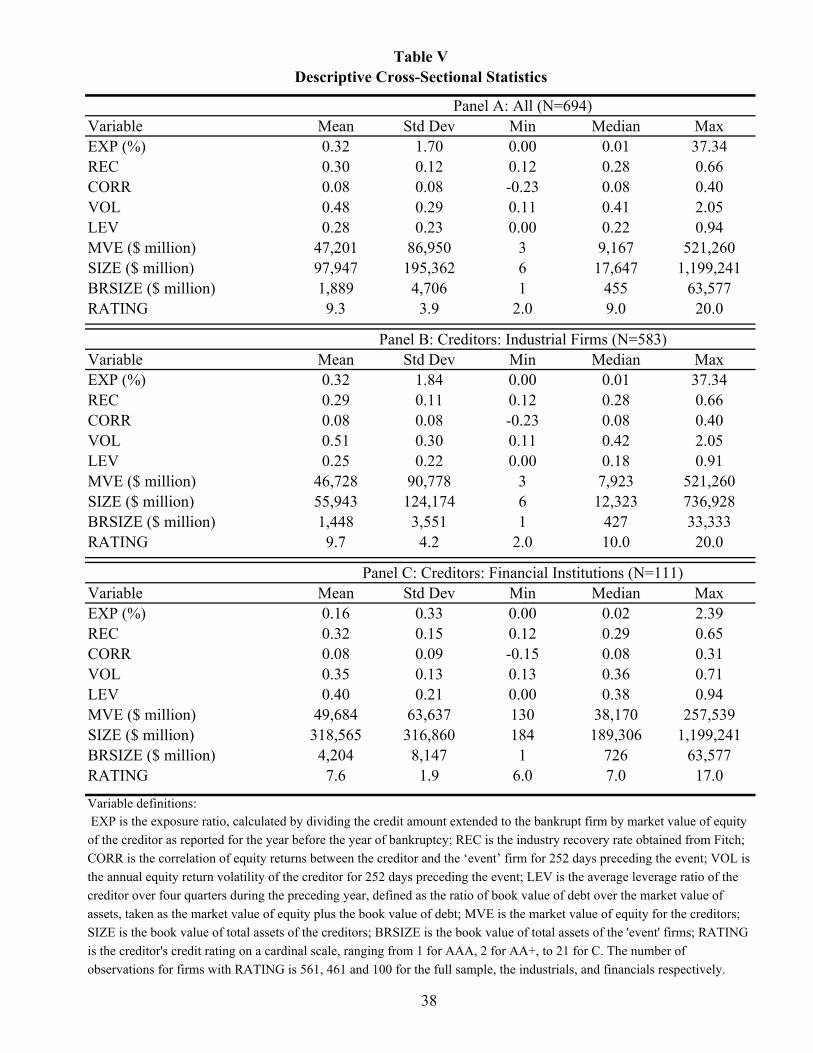
Variable Mean Std Dev Min Median MaxEXP (%) 0.32 1.70 0.00 0.01 37.34REC 0.30 0.12 0.12 0.28 0.66CORR 0.08 0.08 -0.23 0.08 0.40VOL 0.48 0.29 0.11 0.41 2.05LEV 0.28 0.23 0.00 0.22 0.94MVE ($ million) 47,201 86,950 3 9,167 521,260SIZE ($ million) 97,947 195,362 6 17,647 1,199,241BRSIZE ($ million) 1,889 4,706 1 455 63,577RATING 9.3 3.9 2.0 9.0 20.0

Variable Mean Std Dev Min Median MaxEXP (%) 0.32 1.84 0.00 0.01 37.34REC 0.29 0.11 0.12 0.28 0.66CORR 0.08 0.08 -0.23 0.08 0.40VOL 0.51 0.30 0.11 0.42 2.05LEV 0.25 0.22 0.00 0.18 0.91MVE ($ million) 46,728 90,778 3 7,923 521,260SIZE ($ million) 55,943 124,174 6 12,323 736,928BRSIZE ($ million) 1,448 3,551 1 427 33,333RATING 9.7 4.2 2.0 10.0 20.0

Variable Mean Std Dev Min Median MaxEXP (%) 0.16 0.33 0.00 0.02 2.39REC 0.32 0.15 0.12 0.29 0.65CORR 0.08 0.09 -0.15 0.08 0.31VOL 0.35 0.13 0.13 0.36 0.71LEV 0.40 0.21 0.00 0.38 0.94MVE ($ million) 49,684 63,637 130 38,170 257,539SIZE ($ million) 318,565 316,860 184 189,306 1,199,241BRSIZE ($ million) 4,204 8,147 1 726 63,577RATING 7.6 1.9 6.0 7.0 17.0

Variable definitions:

38

Panel A: All (N=694)

EXP is the exposure ratio, calculated by dividing the credit amount extended to the bankrupt firm by market value of equity of the creditor as reported for the year before the year of bankruptcy; REC is the industry recovery rate obtained from Fitch; CORR is the correlation of equity returns between the creditor and the ‘event’ firm for 252 days preceding the event; VOL is the annual equity return volatility of the creditor for 252 days preceding the event; LEV is the average leverage ratio of the creditor over four quarters during the preceding year, defined as the ratio of book value of debt over the market value of assets, taken as the market value of equity plus the book value of debt; MVE is the market value of equity for the creditors; SIZE is the book value of total assets of the creditors; BRSIZE is the book value of total assets of the 'event' firms; RATING is the creditor's credit rating on a cardinal scale, ranging from 1 for AAA, 2 for AA+, to 21 for C. The number of observations for firms with RATING is 561, 461 and 100 for the full sample, the industrials, and financials respectively.

Table VDescriptive Cross-Sectional Statistics

Panel B: Creditors: Industrial Firms (N=583)

Panel C: Creditors: Financial Institutions (N=111)

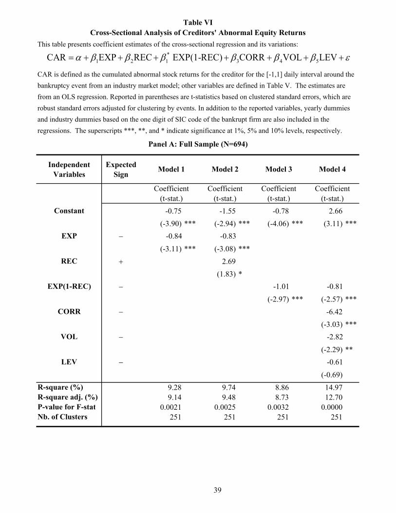
Independent Variables

Expected Sign

Constant -0.75 -1.55 -0.78 2.66(-3.90) *** (-2.94) *** (-4.06) *** (3.11) ***

EXP − -0.84 -0.83(-3.11) *** (-3.08) ***

REC + 2.69(1.83) *

EXP(1-REC) − -1.01 -0.81(-2.97) *** (-2.57) ***

CORR − -6.42(-3.03) ***

VOL − -2.82(-2.29) **

LEV − -0.61(-0.69)

R-square (%) 9.28 9.74 8.86 14.97R-square adj. (%) 9.14 9.48 8.73 12.70P-value for F-stat 0.0021 0.0025 0.0032 0.0000Nb. of Clusters 251 251 251 251

39

(t-stat.)Coefficient

(t-stat.)(t-stat.)Coefficient

(t-stat.)Coefficient Coefficient

Table VI

CAR is defined as the cumulated abnormal stock returns for the creditor for the [-1,1] daily interval around the bankruptcy event from an industry market model; other variables are defined in Table V. The estimates are from an OLS regression. Reported in parentheses are t-statistics based on clustered standard errors, which are robust standard errors adjusted for clustering by events. In addition to the reported variables, yearly dummies and industry dummies based on the one digit of SIC code of the bankrupt firm are also included in the regressions. The superscripts ***, **, and * indicate significance at 1%, 5% and 10% levels, respectively.

Panel A: Full Sample (N=694)

Model 3Model 2Model 1

This table presents coefficient estimates of the cross-sectional regression and its variations:Cross-Sectional Analysis of Creditors' Abnormal Equity Returns

Model 4

*1 2 1 3 4 5CAR EXP REC EXP(1-REC) CORR VOL LEVα β β β β β β ε= + + + + + + +

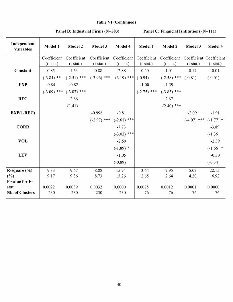
Independent Variables

Constant -0.85 -1.63 -0.88 2.88 -0.20 -1.01 -0.17 -0.01(-3.84) ** (-2.51) *** (-3.96) *** (3.19) *** (-0.94) (-2.58) *** (-0.81) (-0.01)

EXP -0.84 -0.82 -1.00 -1.39(-3.09) *** (-3.07) *** (-2.75) *** (-3.83) ***

REC 2.66 2.67(1.41) (2.40) ***

EXP(1-REC) -0.996 -0.81 -2.09 -1.91(-2.97) *** (-2.61) *** (-4.07) *** (-1.77) *

CORR -7.73 -3.89(-3.02) *** (-1.36)

VOL -2.59 -2.39(-1.89) * (-1.66) *

LEV -1.05 -0.30(-0.89) (-0.34)

R-square (%) 9.33 9.67 8.88 15.94 3.64 7.95 5.07 22.15(%) 9.17 9.36 8.73 13.26 2.65 2.64 4.20 6.92P-value for F-stat 0.0022 0.0039 0.0032 0.0000 0.0075 0.0012 0.0001 0.0000Nb. of Clusters 230 230 230 230 76 76 76 76

40

Panel C: Financial Isntitutions (N=111)

(t-stat.)

Panel B: Industrial Firms (N=583)

Coefficient(t-stat.)

Coefficient(t-stat.)

Model 1 Model 3Model 2

Table VI (Continued)

(t-stat.) (t-stat.) (t-stat.) (t-stat.)Coefficient Coefficient Coefficient

(t-stat.)Coefficient Coefficient

Model 2

Coefficient

Model 1 Model 4Model 4 Model 3

0123jjj jjjjjCACSCORRLEV LHERFDIPDIαβββ βββε=+++ ++++

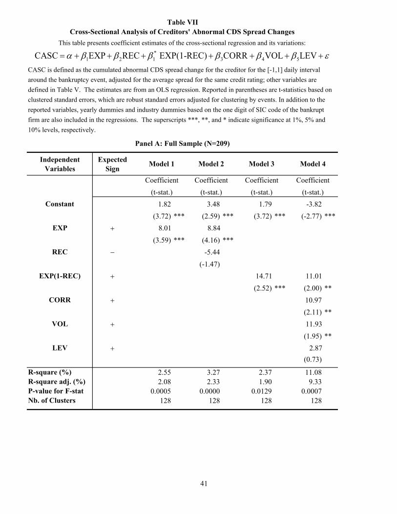
Independent Variables

Expected Sign

Constant 1.82 3.48 1.79 -3.82(3.72) *** (2.59) *** (3.72) *** (-2.77) ***

EXP + 8.01 8.84(3.59) *** (4.16) ***

REC − -5.44(-1.47)

EXP(1-REC) + 14.71 11.01(2.52) *** (2.00) **

CORR + 10.97(2.11) **

VOL + 11.93(1.95) **

LEV + 2.87(0.73)

R-square (%) 2.55 3.27 2.37 11.08R-square adj. (%) 2.08 2.33 1.90 9.33P-value for F-stat 0.0005 0.0000 0.0129 0.0007Nb. of Clusters 128 128 128 128

41

Coefficient

CASC is defined as the cumulated abnormal CDS spread change for the creditor for the [-1,1] daily interval around the bankruptcy event, adjusted for the average spread for the same credit rating; other variables are defined in Table V. The estimates are from an OLS regression. Reported in parentheses are t-statistics based on clustered standard errors, which are robust standard errors adjusted for clustering by events. In addition to the reported variables, yearly dummies and industry dummies based on the one digit of SIC code of the bankrupt firm are also included in the regressions. The superscripts ***, **, and * indicate significance at 1%, 5% and 10% levels, respectively.

Panel A: Full Sample (N=209)

Model 3Model 2 Model 4

Coefficient(t-stat.)

Model 1

Coefficient(t-stat.) (t-stat.)(t-stat.)

Coefficient

Table VIICross-Sectional Analysis of Creditors' Abnormal CDS Spread Changes

This table presents coefficient estimates of the cross-sectional regression and its variations:*

1 2 1 3 4 5CASC EXP REC EXP(1-REC) CORR VOL LEVα β β β β β β ε= + + + + + + +

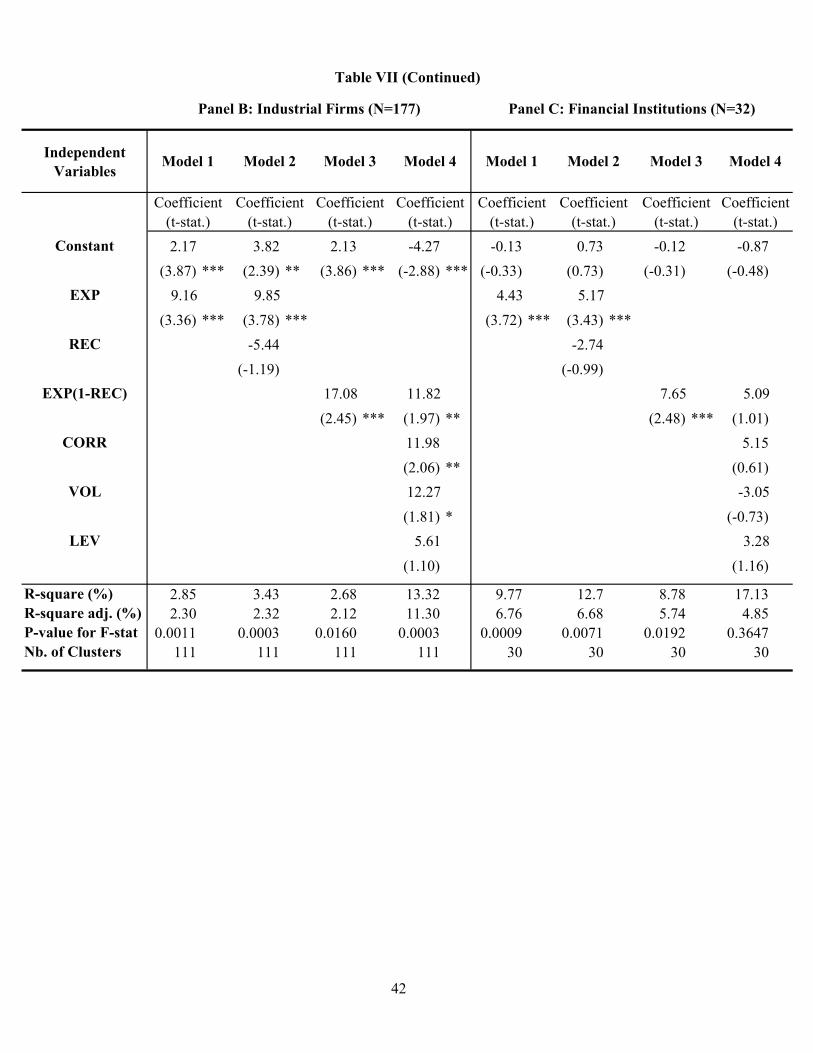
Independent Variables

Constant 2.17 3.82 2.13 -4.27 -0.13 0.73 -0.12 -0.87(3.87) *** (2.39) ** (3.86) *** (-2.88) *** (-0.33) (0.73) (-0.31) (-0.48)

EXP 9.16 9.85 4.43 5.17(3.36) *** (3.78) *** (3.72) *** (3.43) ***

REC -5.44 -2.74(-1.19) (-0.99)

EXP(1-REC) 17.08 11.82 7.65 5.09(2.45) *** (1.97) ** (2.48) *** (1.01)

CORR 11.98 5.15(2.06) ** (0.61)

VOL 12.27 -3.05(1.81) * (-0.73)

LEV 5.61 3.28(1.10) (1.16)

R-square (%) 2.85 3.43 2.68 13.32 9.77 12.7 8.78 17.13R-square adj. (%) 2.30 2.32 2.12 11.30 6.76 6.68 5.74 4.85P-value for F-stat 0.0011 0.0003 0.0160 0.0003 0.0009 0.0071 0.0192 0.3647Nb. of Clusters 111 111 111 111 30 30 30 30

42

(t-stat.)

Model 4

(t-stat.)Coefficient

(t-stat.)Coefficient

(t-stat.)

Model 1

Coefficient

Model 3

Panel C: Financial Institutions (N=32)Panel B: Industrial Firms (N=177)

Coefficient Coefficient

Model 1 Model 2 Model 3

Table VII (Continued)

(t-stat.) (t-stat.) (t-stat.)

Model 4

Coefficient Coefficient

Model 2

Coefficient(t-stat.)

0123jjj jjjjjCACSCORRLEV LHERFDIPDIαβββ βββε=+++ ++++

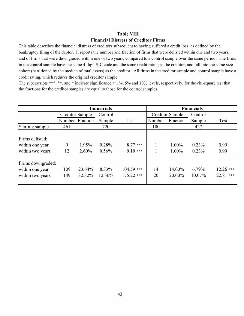
Control ControlNumber Fraction Sample Number Fraction Sample

Starting sample 461 720 100 427

Firms delisted:within one year 9 1.95% 0.28% 8.77 *** 1 1.00% 0.23% 0.99within two years 12 2.60% 0.56% 9.10 *** 1 1.00% 0.23% 0.99

Firms downgraded:within one year 109 23.64% 8.33% 104.59 *** 14 14.00% 6.79% 12.26 ***within two years 149 32.32% 12.36% 175.22 *** 20 20.00% 10.07% 22.81 ***

43

Test Test

Industrials FinancialsCreditor Sample Creditor Sample

This table describes the financial distress of creditors subsequent to having suffered a credit loss, as defined by the bankruptcy filing of the debtor. It reports the number and fraction of firms that were delisted within one and two years, and of firms that were downgraded within one or two years, compared to a control sample over the same period. The firms in the control sample have the same 4-digit SIC code and the same credit rating as the creditor, and fall into the same size cohort (partitioned by the median of total assets) as the creditor. All firms in the creditor sample and control sample have a credit rating, which reduces the original creditor sample.

Financial Distress of Creditor FirmsTable VIII

The superscripts ***, **, and * indicate significance at 1%, 5% and 10% levels, respectively, for the chi-square test that the fractions for the creditor samples are equal to those for the control samples.

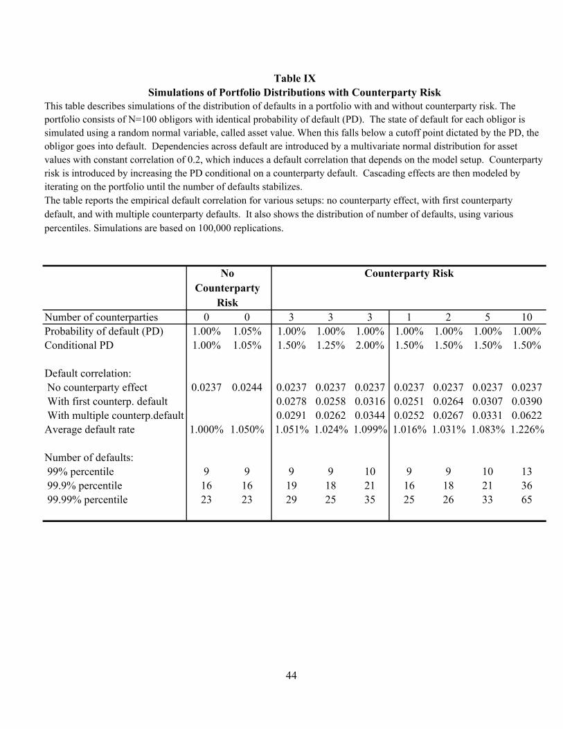
Number of counterparties 0 0 3 3 3 1 2 5 10Probability of default (PD) 1.00% 1.05% 1.00% 1.00% 1.00% 1.00% 1.00% 1.00% 1.00%Conditional PD 1.00% 1.05% 1.50% 1.25% 2.00% 1.50% 1.50% 1.50% 1.50%

Default correlation: No counterparty effect 0.0237 0.0244 0.0237 0.0237 0.0237 0.0237 0.0237 0.0237 0.0237 With first counterp. default 0.0278 0.0258 0.0316 0.0251 0.0264 0.0307 0.0390 With multiple counterp.default 0.0291 0.0262 0.0344 0.0252 0.0267 0.0331 0.0622Average default rate 1.000% 1.050% 1.051% 1.024% 1.099% 1.016% 1.031% 1.083% 1.226%

Number of defaults: 99% percentile 9 9 9 9 10 9 9 10 13 99.9% percentile 16 16 19 18 21 16 18 21 36 99.99% percentile 23 23 29 25 35 25 26 33 65

44

Counterparty Risk

This table describes simulations of the distribution of defaults in a portfolio with and without counterparty risk. The portfolio consists of N=100 obligors with identical probability of default (PD). The state of default for each obligor is simulated using a random normal variable, called asset value. When this falls below a cutoff point dictated by the PD, the obligor goes into default. Dependencies across default are introduced by a multivariate normal distribution for asset values with constant correlation of 0.2, which induces a default correlation that depends on the model setup. Counterparty risk is introduced by increasing the PD conditional on a counterparty default. Cascading effects are then modeled by iterating on the portfolio until the number of defaults stabilizes.

Simulations of Portfolio Distributions with Counterparty RiskTable IX

The table reports the empirical default correlation for various setups: no counterparty effect, with first counterparty default, and with multiple counterparty defaults. It also shows the distribution of number of defaults, using various percentiles. Simulations are based on 100,000 replications.

No Counterparty

Risk