Credit Risk Factor Modelingand the Basel II IRB Approach

Alfred Hamerle(University of Regensburg)

Thilo Liebig(Deutsche Bundesbank)

Daniel R�sch(University of Regensburg)

Discussion PaperSeries 2: Banking and Financial SupervisionNo 02/2003

Discussion Papers represent the authors’ personal opinions and do not necessarily reflect the views of theDeutsche Bundesbank or its staff.

Editorial Board: Heinz HerrmannThilo LiebigKarl-Heinz Tödter

Deutsche Bundesbank, Wilhelm-Epstein-Strasse 14, 60431 Frankfurt am Main,Postfach 10 06 02, 60006 Frankfurt am Main

Tel +49 69 9566-1Telex within Germany 41227, telex from abroad 414431, fax +49 69 5601071

Please address all orders in writing to: Deutsche Bundesbank,Press and Public Relations Division, at the above address or via fax No +49 69 9566-3077

Reproduction permitted only if source is stated.

ISBN 3–935821–70–0

Credit Risk Factor Modeling and the Basel II IRB Approach*

Abstract

Default probabilities (PDs) and correlations play a crucial role in the New Basel Capital Accord. In commercial

credit risk models they are an important constituent. Yet, modeling and estimation of PDs and correlations is still

under active discussion. We show how the Basel II one factor model which is used to calibrate risk weights can

be extended to a model for estimating PDs and correlations. The important advantage of this model is that it uses

actual information about the point in time of the credit cycle. Thus, uncertainties about the parameters which are

needed for Value-at-Risk calculations in portfolio models may be substantially reduced. First empirical evidence

for the appropriateness of the models and underlying risk factors is given with S&P data.

Keywords: Credit Risk, Credit Ratings, Probability of Default, Bank RegulationJEL Classification: C1, G21

* This paper was presented in October 2002 on the 9th annual meeting of the German Finance Association in

Cologne. We thank the participants of the conference for helpful suggestions.

Zusammenfassung

Ausfallwahrscheinlichkeiten (PDs) und Korrelationen spielen eine entscheidende Rolle in den geplanten neuen

Eigenmittelvereinbarungen (Basel II). Des Weiteren sind sie ein wichtiger Bestandteil von Kreditrisikomodellen.

Dennoch existieren bei der Modellierung und Schätzung von PDs noch viele offene Fragen. Wir zeigen in die-

sem Papier wie das Ein-Faktor-Modell, das im Rahmen von Basel II zur Kalibrierung der Risikogewichte ver-

wendet wird, erweitert werden kann, um die Schätzung von PDs und Korrelationen zu ermöglichen. Der

entscheidende Vorteil dieses Modells besteht darin, dass es die jeweils aktuelle Information über den Stand des

Konjunkturzykluses verwendet. Auf diese Weise können die Unsicherheiten über die Parameter, die für die Be-

rechnung des Value-at-Risks in Portfoliomodellen benötigt werden, deutlich reduziert werden. Mit Hilfe von

Daten von S&P wird die Angemessenheit des Modells und der zugrundeliegenden Riskofaktoren empirisch

untersucht.

Schlagwörter: Kreditrisiko, Ratingverfahren, Ausfallwahrscheinlichkeit, Bank RegulierungJEL Klassifizierung: C1, G21

Contents

1 Introduction 1

2 Default Event, Asset Value, and Default Probability 3

3 The Basel II Model and a Generalized Factor Model Representation 5

3.1 The Basel II Model for Asset Returns 5

3.2 Factor Models for Stock Returns 8

3.2.1 Statistical Factor Models 8

3.2.2 Macroeconomic or Index Factor Models 9

3.2.3 Fundamental Factor Models 10

3.3 A Generalized Factor Model for Credit Risk 11

4 A Factor Model Representation for Default Data 12

5 Empirical Evidence and Implications for Risk Management and the Basel II

IRB Approach 15

6 Summary and Conclusion 19

1

1 Introduction

In the light of permanently growing default rates and diminishing margins the measure-ment and controlling of credit risk is essential – especially in the field of corporate bank-ing. This is also stated by the Basel Committee on Banking Supervision who published athird consultative document in April 2003. The paper was followed by the EuropeanCommission’s third consultative document in July 2003 which essentially adopted theBasel notions.

The Basel documents (1999a, 1999b, 2000, 2001, 2003) describe several determinants ofdefault risk, i.e. the Default Probability (PD), the Loss Given Default, the Exposure AtDefault, the Maturity, and Correlations. Modeling of PDs and correlations is stated as akey factor for credit risk models since value-at-risk calculations are very sensitive due tochanges in these parameters. In many credit risk models such as CreditMetrics, Credi-tRisk+ or CreditPortfolioView, default probabilities are essential input parameters. Foroutlines of these models see Gupton et al. (1997), Credit Suisse Financial Products(1997), and Wilson (1997a, 1997b). Approaches for unifying the different credit riskmodels are found in Gordy (1998), Koyluoglu/Hickman (1998), and Crouhy et al. (2000).

In the literature on credit risk several different approaches for modeling default prob-abilities are suggested. These approaches use different assumptions and informationwhich is not always available for every firm. The asset value model due to Merton (1974)and Black/Scholes (1973)1 assumes that the market value of total assets is observable inprinciple. Furthermore the capital structure is explicitly considered and default happens ifthe value of total assets is lower than the value of liabilities. In contrast reduced formmodels and other spread-related approaches derive relations between the credit spread ofthe credit risky bond and the default probability (e.g., Jarrow/Turnbull, 1995, Duf-fie/Singleton, 1997 and 1999, Madan/Unal, 1998, and Lando, 1998). An essential part ofthe theory of these models is the risk neutral valuation under the absence of arbitrage op-portunities. Therefore the existence of market prices is indispensable for practical appli-cations (see Jarrow/Turnbull, 2000).

1 Extensions of the model can be found in Black/Cox (1976), Merton (1977), Geske (1977), Long-staff/Schwartz (1995), and Zhou (2001).

2

Another class of models, especially for mid-size corporate customers which do not offermarket prices use rating procedures for the assessment of credit quality. For an outline ofthese models see Jarrow/Lando/Turnbull (1997) and Altman/Saunders (1998). Accordingto the rating a segmentation in homogenous rating grades is employed. For each grade adefault rate is determined and it is assumed that all borrowers within a grade exhibit equaldefault probabilities. The default probability is estimated by the default rate of eachgrade, sometimes after calculating historical averages.

A recent approach of a generalized framework for credit risk models and for defaultprobabilities is due to Koyluoglu/Hickman (1998). These authors consider approacheswhich are used in current credit risk models, i.e. the “market factor model” from Credit-Metrics, the “default rate model” from CreditPortfolioView and the “probability generat-ing model” from CreditRisk+. In these approaches the variation of the default probabilitycan be attributed to one or more “systemic” factors which are randomly drawn from thesame distribution at each point in time.

Regarding default correlations mainly one of two directions is followed. The first onemodels default correlations between two borrowers directly by assuming a two-dimensional correlated Brownian motion for the returns on the values of the firms’ assetswhich trigger the defaults. The second direction, see e.g. CreditPortfolioView or Credi-tRisk+, models correlations by borrowers’ exposures to common risk factors. Given therealizations of the risk factors, asset returns and, thus, defaults are uncorrelated. The ideabehind the Basel II model follows this direction by assuming the existence of one non-observable contemporaneous risk factor which is responsible for correlations.

The purpose of the present paper is to extend the Basel II framework to a model whichdirectly relates observable risk factors to the Basel II model. Thus, default correlationsand, furthermore, default probabilities can be directly attributed to the risk factors.

First, the outline of the model which underlies the Basel II Accord is summarized. It isshown that it can be extended to a general approach in a way that allows not only forchanges of the conditional PD which is due to a common unobservable random factorunder the assumption of a constant unconditional PD. Rather it also allows for changes ofunconditional PDs due to observable risk factors. This extends the existing models to adynamic setting. Koyluoglu/Hickman (1998), Lucas et al. (2000) and others describemodel set-ups that are static in the sense that the risk factors which drive default rates orrating migrations are assumed i.i.d. Here we explicitly allow for time dependency of un-conditional PDs in a multi-period model.

3

Second, it is shown that these observable risk factors can be identified by using a gener-alization of factor models for stock returns which are widely used in the financial area.This combination allows for modeling the systematic changes of the unconditional PDsand the random changes of the conditional PDs simultaneously.

Third, it is shown how these combined factor models can be employed even if stock re-turns are unobservable and rather only default data are observable. This is important es-pecially for small and medium firms which do not have any marketable assets. Thus, themodel is an example for how PDs can be estimated within the Basel II IRB framework. Itis shown that an appropriate threshold model connecting the unobservable returns on afirm’s assets with the observable default event leads to random effects logit or probit re-gression models which are extensions of the Basel II model.

Finally, consequences for portfolio modeling in the extended Basel II model are dis-cussed. It is shown how knowledge about the relevant risk factors influences the parame-ters and reduces asset and default correlations. Thus, generating loss distributions can besimplified and become easier to handle. The model is demonstrated by analyzing empiri-cal ratings data from 1982 to 1999.

The paper proceeds as follows. Section 2 defines the default event. In section 3 the BaselII model, common factor models for stock returns and a combination of them which isconsistent with Basel II are discussed. Section 4 shows how these models are extended tothe case when only default data are available. Section 5 discusses the implications forportfolio models and risk management and offers empirical evidence. Section 6 providesthe summary and the conclusion.

2 Default Event, Asset Value, and Default Probability

In probabilistic terms the default event is random. Any attempt to quantifying credit riskhas to determine the probability of the default event (PD) within a given future time pe-riod.2

Below the subscript t denotes the actual time and a single period is considered – e.g. oneyear. The two possible states at time t for borrower i, i=1,...,N, “default” and “non-default” are modeled by the indicator variable *

itY with

2 In addition, other parameters, such as Exposure At Default (EAD) or Loss Given Default (LGD) are

necessary. The primary focus of this paper is on PD and correlations and we treat the other parametersas known.

4

���

�else0

in defaults borrower 1 tiYit*

Consider a continuous-state variable itY which may be interpreted as the natural loga-

rithm of the value of the firm’s assets. The default event is equivalent to the value of afirm’s assets crossing a threshold itc at t , i.e.

1���*ititit YcY (* 1).

The one-period default probabilities can be characterized by successively building up athreshold model. The model is formulated in a discrete time setting. The successive pro-gression results from the fact that the process of the asset value only reaches time t ifdefault has not taken place until time 1�t . Else the firm is liquidated and the process ofthe asset value terminates. This conditional probability of the asset value falling belowthe threshold at time t , given survival until time 1�t , is denoted by

� �11 ����� ititititit cYcYP� . (* 2)

Equivalently the „time to default“ iT could be treated as the relevant random variable.Here, iT is an integer variable since only whole periods are counted. tTi � means thatdefault happens at time t , the condition 1�� tTi means that firm i did not default before

t . The conditional default probability

� �1���� tTtTP iiit� (* 3)

is also called a discrete-time hazard rate.3

3 Usually hazard rates are analyzed in continuous-time settings, especially in biometrics and reliability

theory. In the field of stochastic processes an extension is often found by stochastic intensity models,which play an important role in reduced-form-models (see, for example, Jarrow/Turnbull, 2000, orLando, 1998). Our focus, however, is on the discrete-time setting with a larger time horizon, e.g. oneyear, which is generally used by bank practitioners (see Basel Committee on Banking Supervision, 2001and 2003). As it is common in biometrics we adopt the term hazard rate for the discrete-time setting (seeKalbfleisch/Prentice, 1980, chap. 2.4).

5

While it always can be assumed that the default event is observable, the observability ofthe value of a firm’s assets itY depends on the available data. If the asset value is observ-

able, for example if market values of equity or credit scores are used as proxies, then themodel is linear. Otherwise a nonlinear model is estimated which treats the asset value as alatent variable. In the following section the common framework for both cases is pre-sented.

3 The Basel II Model and a Generalized Factor Model Representation

3.1 The Basel II Model for Asset Returns

As it is common in finance the asset value itself is not modeled. Rather a model is builtfor the changes, i.e. the returns, on the logarithm of a firm’s assets. The return on bor-rower i’s assets at time t is represented by the normal distributed random variable

� �21 iitititit NyYR �� ,~

��� (* 4)

(i=1,…,N; t=1,...,T), where � � ititit yRE ���1 and � � 2

1Var iitit yR ���

are mean and

standard deviation respectively. In the Basel II model it is assumed that deviations of as-set returns from their means are due to a factor model with one systematic factor tFwhich affects all returns simultaneously and N idiosyncratic factors itU which affect each

return separately. The exposure b to the common factor is equal for all firms within agiven risk segment (for example, industry or size), i.e.4

ittitit UFbR �� ��� (* 5)

where

� �10,~ NFt , � �10,~ NUit

4 Note that in the Basel II model the subscript “t” is not taken into account. Rather, standardized returns

are directly modeled. Thus, model (* 5) with time-dependent it� represents an extension which hasimportant implications for credit risk modeling throughout the paper.

6

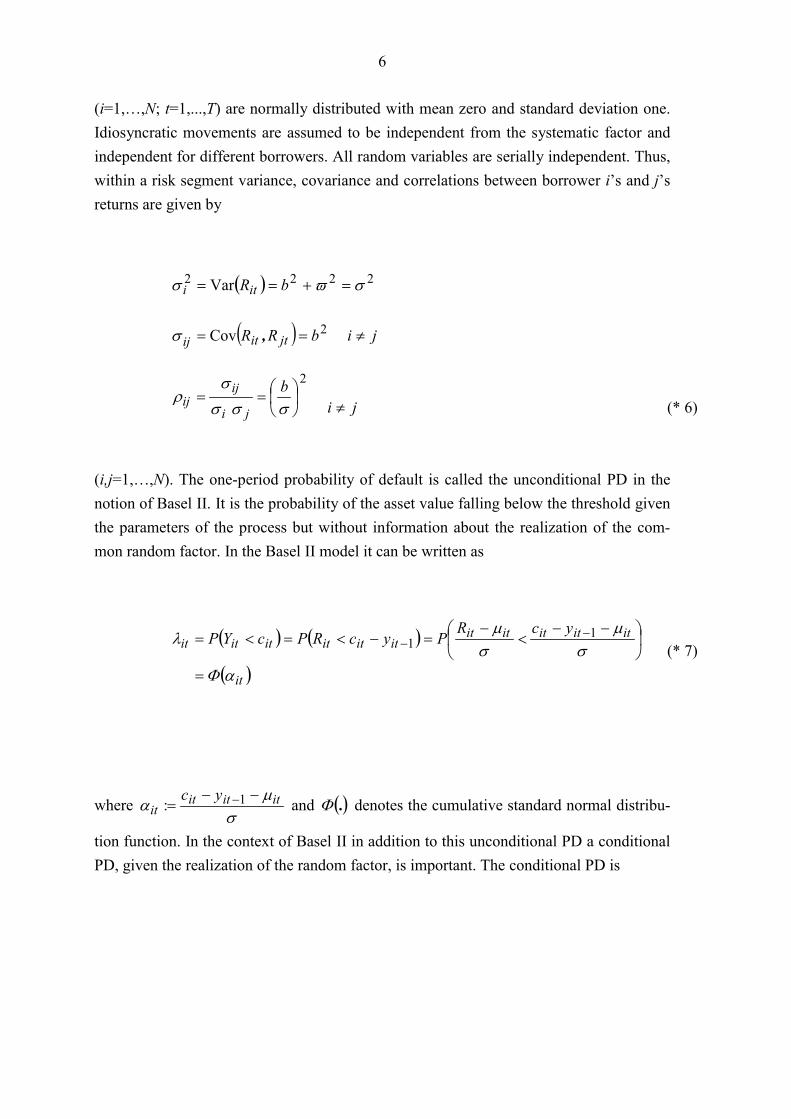
(i=1,…,N; t=1,...,T) are normally distributed with mean zero and standard deviation one.Idiosyncratic movements are assumed to be independent from the systematic factor andindependent for different borrowers. All random variables are serially independent. Thus,within a risk segment variance, covariance and correlations between borrower i’s and j’sreturns are given by

� � 2222 Var ��� ���� bRiti

� � 2Cov bRR jtitij �� ,� ji �

2��

���

���

���

��

b

ji

ijij ji � (* 6)

(i,j=1,…,N). The one-period probability of default is called the unconditional PD in thenotion of Basel II. It is the probability of the asset value falling below the threshold giventhe parameters of the process but without information about the realization of the com-mon random factor. In the Basel II model it can be written as

� � � �

� �it

ititititititititititit

ycRPycRPcYP

��

�

�

�

��

�

��

���

� ��

����� �

�

11 (* 7)

where �

��

itititit

yc ��

��1: and � �.� denotes the cumulative standard normal distribu-

tion function. In the context of Basel II in addition to this unconditional PD a conditionalPD, given the realization of the random factor, is important. The conditional PD is

7

� �

� �

������

�

�

������

�

�

��

���

��

��

������

�

�

������

�

�

��

���

��

��

��

�

�

��

�

�

��

�

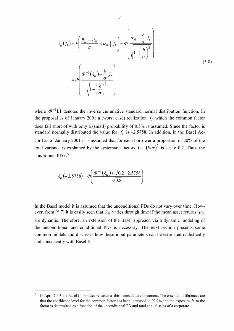
2

1

2

1

1

�

���

�

�

��

���

��

b

fb

b

fb

fR

Pf

tit

tittit

itittit

(* 8).

where � �.1�� denotes the inverse cumulative standard normal distribution function. In

the proposal as of January 2001 a (worst case) realization tf which the common factor

does fall short of with only a (small) probability of 0.5% is assumed. Since the factor isstandard normally distributed the value for tf is –2.5758. In addition, in the Basel Ac-

cord as of January 2001 it is assumed that for each borrower a proportion of 20% of thetotal variance is explained by the systematic factors, i.e. � �2�b is set to 0.2. Thus, the

conditional PD is5

� �� �

��

�

�

��

�

� ��

�

805758220

575821

.... it

it��

��

In the Basel model it is assumed that the unconditional PDs do not vary over time. How-ever, from (* 7) it is easily seen that it� varies through time if the mean asset returns it�

are dynamic. Therefore, an extension of the Basel approach via a dynamic modeling ofthe unconditional and conditional PDs is necessary. The next section presents somecommon models and discusses how these input parameters can be estimated realisticallyand consistently with Basel II.

5 In April 2003 the Basel Committee released a third consultative document. The essential differences are

that the confidence level for the common factor has been increased to 99.9% and the exposure b to thefactor is determined as a function of the unconditional PD and total annual sales of a corporate.

8

3.2 Factor Models for Stock Returns

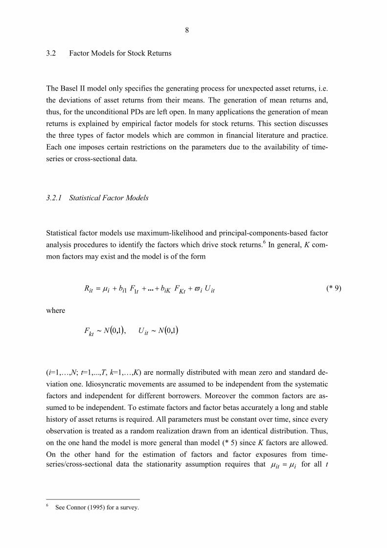
The Basel II model only specifies the generating process for unexpected asset returns, i.e.the deviations of asset returns from their means. The generation of mean returns and,thus, for the unconditional PDs are left open. In many applications the generation of meanreturns is explained by empirical factor models for stock returns. This section discussesthe three types of factor models which are common in financial literature and practice.Each one imposes certain restrictions on the parameters due to the availability of time-series or cross-sectional data.

3.2.1 Statistical Factor Models

Statistical factor models use maximum-likelihood and principal-components-based factoranalysis procedures to identify the factors which drive stock returns.6 In general, K com-mon factors may exist and the model is of the form

itiKtiKtiiit UFbFbR �� ����� ...11 (* 9)

where

� �10,~ NFkt , � �10,~ NUit

(i=1,…,N; t=1,...,T, k=1,…,K) are normally distributed with mean zero and standard de-viation one. Idiosyncratic movements are assumed to be independent from the systematicfactors and independent for different borrowers. Moreover the common factors are as-sumed to be independent. To estimate factors and factor betas accurately a long and stablehistory of asset returns is required. All parameters must be constant over time, since everyobservation is treated as a random realization drawn from an identical distribution. Thus,on the one hand the model is more general than model (* 5) since K factors are allowed.On the other hand for the estimation of factors and factor exposures from time-series/cross-sectional data the stationarity assumption requires that iit �� � for all t

6 See Connor (1995) for a survey.

9

(t=1,..., T). This also means that default probabilities are constant through time. A discus-sion and generalization of this will follow in section 3.3.

3.2.2 Macroeconomic or Index Factor Models

Macroeconomic models or index models use stock indices or observable economic timeseries as factors, such as inflation risk, GDP change or interest rates. In this case the re-gression model is of the form

ititiiit UR �� ��� Z'β0 (* 10)

(i=1,…,N; t=1,...,T), where i0� and iβ are unknown firm specific parameters to be esti-

mated. The seminal reference for this kind of model is Chen/Roll/Ross (1986). For theestimation a time-series regression model is employed where the stationarity assumptions� � � �ZZ EE t � and � � � �ZZ CovCov �t for all t (t=1,..., T) must hold. In this case the ex-

pected asset returns � � � �Z'β ERE iiit �� 0� are time independent. Note also that ex-

pected returns in t conditional on realizations of the risk factors at 1�t� � � �Z'βz ERE iitit ��

� 01 � are also time-independent. Moreover, the asset returns are

assumed to be serially independent.

This model is also found in the CreditMetrics framework where the risk factors are repre-sented by contemporaneous stock index returns. The covariance between the standardizedasset returns of firm i and j, resp. the correlation of asset returns is

� � jiji

ij βZβ' Cov1��

� �

and is due to the exposures to the common observable risk factors or indices. For givenrealizations tt zZ � of the risk factors the returns are independent.

10

3.2.3 Fundamental Factor Models

Fundamental factor models use firm specific information itX as regressors, such as ac-

counting data, firm size or index betas. The regression model is

ittitttit UR �� ��� X'γ0 (* 11)

(i=1,…,N; t=1,...,T). itX are interpreted as observable exposures to respective latent fac-tors where � � � �� �ttit EN XX~X Cov , (i=1,…,N; t=1,...,T). The vector tγ are the ex-

pected returns of mimicking portfolios of the latent factors which are to be estimated bycross-sectional regression. The seminal references for this kind of models areFama/MacBeth (1973) and Fama/French (1992). It is assumed that expected latent factorreturns are constant through time, i.e. γγ �t (t=1,...,T). Thus, the correlation between

asset returns is

� � γXγ' ttt

t Cov1��

� � .

In this model expected asset returns are allowed to vary through time due to the variationof expected factor exposures � �tE X . For given realizations itit xX � of the factor expo-

sures the returns of two assets are independent. Recently these models are also found forexplaining credit spread changes, see Duffee (1998), Pedrosa/Roll (1998) or Collin-Dufresne et al. (2001).

11

3.3 A Generalized Factor Model for Credit Risk

The empirical regression models from section 3.2 describe stock returns either as func-tions of macroeconomic time series or as functions of cross-sectional exposures. If time-series and cross-sectional data are available the models can be combined into one modelwhich uses all information simultaneously. Furthermore this general model can be com-bined with the Basel II model where the existence of one common unobservable factor isassumed in addition. A model which combines fundamental, macroeconomic and statisti-cal factor models is compatible with the Basel II model and it is able to explain thegrowth of firm values (and, thus, PDs) by various risk sources.

We assume that some risk factors affect the asset returns instantaneously and some riskfactors affect the asset returns with a time lag. For example, some management decisionsmay cause a default immediately between 1�t and t while some past decisions have alasting effect on default risk and their consequences are perceived at a later time. Notethat the interpretation of the asset value is not limited to traded assets. Especially, smalland medium firms do not have any traded assets. Markets which process information im-mediately into prices are not available. Therefore, lagged effects on the asset values donot contradict considerations about market efficiency.

Essentially the combined model is a linear random effect panel model. The notationwhich is used below refers to a particular risk segment (for example industry, or sizegroup). It is assumed that the borrowers are homogenous within a risk segment regardingthe relevant risk factors and the factor exposures. The parameters and the risk factors areallowed to differ between segments. Given the information until time t the model for aparticular segment can be written as

ittttitittit UFbR �� ��������� 1211210 z'βZ'βx'γX'γ (* 12)

(i=1,…,N; t=1,...,T), where 11 ββ �i and 22 ββ �i are assumed for all borrowers within

the risk segment. It follows that

� � � � � � 121121011 ,����

����� ttititttitit EERE z'βZ'βx'γX'γzx � .

12

1�itx denotes a corresponding realization of a vector of lagged factors where the sub-script 1�t represents arbitrary lags, i.e. also lags of two or more periods of time. 1�tz is

a corresponding realization of a vector of lagged systematic risk factors. These realiza-tions are known at time t. 1γ , 2γ , 1β and 2β are suitably dimensioned parameter vec-

tors.

For implementation in credit risk modelling proxies for the returns of the firms’ assets areneeded. If stock market data are available these returns can be approximated by stockreturns analogously to CreditMetrics. However, many borrowers of a typical bank portfo-lio do not have any traded assets. Thus, other proxies for asset returns may be employed.The linear panel model can be established, for example with credit scores or credit scorechanges as in Hamerle/Rösch (2001). In general the distribution of the dependent variableat time t depends on the distribution of the risk factors. The goal of model (* 12) is toexplain the dependent variable by lagged factors. Then all realizations of the risk factorsare known at time t , the time-specific intercept vanishes and the distribution at time t isconditional on their lagged realizations. In this case the correlations are due to the randomeffect tF . Furthermore it can be shown that the inclusion of lagged risk factors may su-

persede the random effect. Then conditional on all information at time t the dependentvariables, and thus defaults, are independent. First empirical evidence for this model isgiven in Hamerle/Rösch (2001) where one lagged risk factor is able to explain much ofthe correlation in a sample of credit scores of German firms between 1989 and 1998.

Another possibility of estimation is to treat asset returns as latent variables which are notobservable. Then, information must be gathered from observed default data. This leads tohazard-rate models which are discussed in the next section.

4 A Factor Model Representation for Default Data

In the latent model the realizations of the asset returns are not observable. Only the riskfactors and the realization of the default indicator *

ity are observable. Of interest is the

PD in period t . The link between risk factors and PD is described by the threshold model(* 2). The model is usually formulated for given realizations of the risk factor and thefactor exposures. For convenience, itx , 1�itx , tz and 1�tz are collected in the vector

itw , and correspondingly the parameter vectors 1γ , 2γ , 1β and 2β are collected in δ .Thus the linear term 121121 ��

��� ttitit z'βz'βx'γx'γ is abbreviated by itw'δ . Given

13

that default has not happened before t one obtains for the conditional probability of de-fault (CPD) (given information about the observable factors and factor exposures untiltime period 1�t and given the realization tf of the random factor for time period t )

� � � �

� �tittitit

tittittitit

it

titittitit

ffbF

ffbyc

UP

fYPf

,

,

,1

0

01

w~w'δ~~

ww'δ

w,w *

���

��

���

�����

��

�

�

�

�

�

(* 13)

where �

�� titit

ityc 01

0 :��

��

~ , �

δδ~ ��: and �

bb �

~ represent reparameterizations of

the regression parameters and F denotes the distribution function of the error term itU .Neither the thresholds itc nor the latent values 1�ity can be observed. So firm and timespecific intercepts cannot be estimated. We restrict the intercept to t0� and, for conven-ience, we use again the notation t0� , b and δ for the regression parameters.

Different assumptions about the error distribution function F lead to different models forthe probability of default. The model underlying in Basel II is a random effects probitspecification

� � � �titttitit fbf ��� w'δ,w 0��� (* 14)

It is easily seen that (*14) is an extension of the Basel II model in (* 8) or (* 7) respec-tively. In (* 14) a generalized factor model for the expected return on a firm’s assets isincorporated explaining the firm and time specific variations. A more tractable specifica-tion, which is widely used in applications of categorical regression models, is the logisticspecification. The logistic model can be written as

� �� �� �

� �titt

titt

titttitit

fbL

fbfb

f

���

���

��

�

w'δ

w'δw'δ,w

0

0

0exp1

exp

�

�

��

(* 15)

where � � � � � �� �sssL exp1exp �� . The “unconditional” probability of default (in Basel IIterminology, meaning that we have only information about itw but not about tf ) is

given by

14

� � � � � ����

��

��� tttittitit dfffbF ��� w'δw 0 (* 16)

where � �.� denotes the density function of the standard normal distribution. For example,

for the logistic specification (* 15) one obtains

� � � � � ����

��

��� tttittitit dfffbL ��� w'δw 0 (* 17).

In order to calculate the default correlations we consider again the linear random effectpanel model (* 12) for the returns of a firm’s assets. The linear term

121121 ����� ttitit z'βz'βx'γx'γ is again abbreviated by itw'δ . Then, for given values

of itw , the asset correlation � , i.e. the correlation between itR and jtR ( ji � ) within

the risk segment is given by

22

2

�

�

�

�

bb .

Moreover, for a given realization of the random factor tf the returns itR and jtR are

independent.

Since defaults are binary events the default correlations are determined by the probability

� � � �jtitjtitjtitijt YYP w,w,w,w ** 11 ����

of joint defaults of borrowers i and j. Using (* 16) and the fact that for given tf the de-

faults of borrowers i and j are independent, this joint probability is given by

� � � � � � � ����

��

����� tttjtttittjtitijt dfffbFfbF ���� w'δw'δw,w 00 (* 18).

Whereas the asset correlations between the returns for two firms within a risk segment areequal, this is no longer true for the corresponding default correlations which depend onthe values of itw and jtw respectively. Furthermore, it should be noted that the variance

15

2b of the random effect plays a major role for the default correlation. If 2b is not signifi-cantly different from zero, the random time effect may be neglected. Then, the defaultevents within a risk segment may be considered (conditionally) independent.

5 Empirical Evidence and Implications for Risk Management and the Basel IIIRB Approach

In this section empirical evidence about the generalized model is provided. Since longhistories of real default data are scarce, we use ratings data from 1982 to 1999 from Stan-dard & Poor’s (2001b) which provide firm counts and defaults for seven rating gradesfrom AAA to CCC.

For risk management and determining required capital in the context of Basle II, knowl-edge about the probability distribution of future losses, i.e. the losses which may arise inthe next period 1�t , is needed. Important input parameters for the loss distribution arethe default probabilities 1�it� and the default correlations � �** , 11 �� jtit YY� .

Firstly, we consider the Basel II model without explanatory risk factors. The model inGordy/Heitfield (2000) for estimating asset correlations for rating grades is essentially arandom effects probit model similar to (* 5). It is a one-factor model for the normalizedi.i.d. returns itR~ on a firm’s assets, i.e.

ittit UFR �� ��� 1~ (* 19)

where � � iititit RR ����

~ and � as in (* 6). Again, it is assumed that a firm defaults if

the return on its assets crosses a threshold. For each grade g it is assumed that there is athreshold g0� so that � �g0�� is the unconditional PD of the grade. In comparison to

(* 7) it is assumed that obligors within a grade are treated as homogeneous, and the re-striction is imposed that each grade possesses an unconditional PD which does not de-pend on time. The model is estimated for the whole sample and for the particular ratinggrades.7

7 Since the number of defaults in grades AAA to BBB is too small, the correlation parameter could not be

estimated.

16

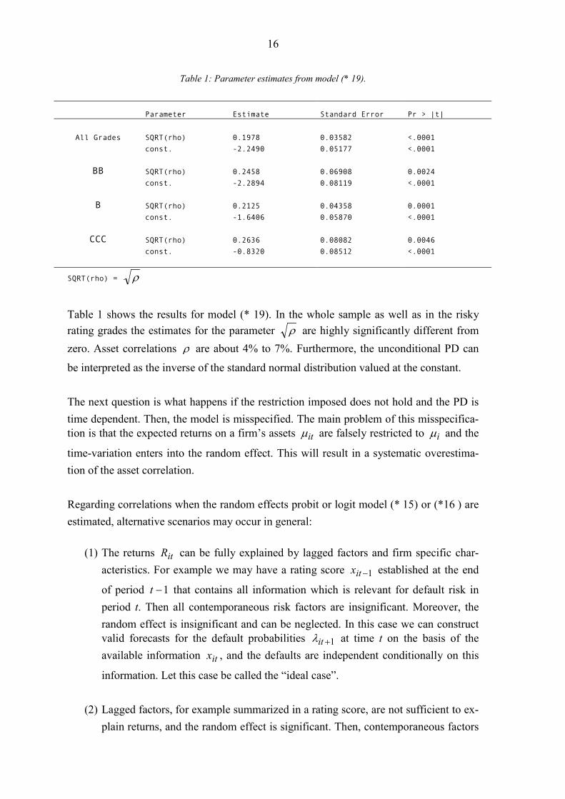
Table 1: Parameter estimates from model (* 19).

Parameter Estimate Standard Error Pr > |t|

All Grades SQRT(rho) 0.1978 0.03582 <.0001const. -2.2490 0.05177 <.0001

BB SQRT(rho) 0.2458 0.06908 0.0024const. -2.2894 0.08119 <.0001

B SQRT(rho) 0.2125 0.04358 0.0001const. -1.6406 0.05870 <.0001

CCC SQRT(rho) 0.2636 0.08082 0.0046const. -0.8320 0.08512 <.0001

SQRT(rho) = �

Table 1 shows the results for model (* 19). In the whole sample as well as in the riskyrating grades the estimates for the parameter � are highly significantly different fromzero. Asset correlations � are about 4% to 7%. Furthermore, the unconditional PD can

be interpreted as the inverse of the standard normal distribution valued at the constant.

The next question is what happens if the restriction imposed does not hold and the PD istime dependent. Then, the model is misspecified. The main problem of this misspecifica-tion is that the expected returns on a firm’s assets it� are falsely restricted to i� and the

time-variation enters into the random effect. This will result in a systematic overestima-tion of the asset correlation.

Regarding correlations when the random effects probit or logit model (* 15) or (*16 ) areestimated, alternative scenarios may occur in general:

(1) The returns itR can be fully explained by lagged factors and firm specific char-acteristics. For example we may have a rating score 1�itx established at the end

of period 1�t that contains all information which is relevant for default risk inperiod t. Then all contemporaneous risk factors are insignificant. Moreover, therandom effect is insignificant and can be neglected. In this case we can constructvalid forecasts for the default probabilities 1�it� at time t on the basis of theavailable information itx , and the defaults are independent conditionally on this

information. Let this case be called the “ideal case”.

(2) Lagged factors, for example summarized in a rating score, are not sufficient to ex-plain returns, and the random effect is significant. Then, contemporaneous factors

17

can be taken into the model, and their inclusion may render the random effect in-significant. In this case forecasts or stochastic models for the contemporaneousrisk factors are needed. Alternatively one could explain as much as possible bylagged factors and keep the random effect in the model. In either case there is afurther source of uncertainty which increases variances in comparison to case (1)and leads to correlations.

(3) As a modification of case (2) one puts the cyclicality into a time-specific interceptt0� . Then the random effect should vanish. Here again, similar to case (2), one

has the problem of forecasting 10 �t� .

(4) As a further modification one can include a rating score 1�itx and a lagged proxy

for the macroeconomic environment, for example the overall default rates of time1�t for explaining returns. If the intercept of the resulting model does not depend

on time and the random effect is not significant one has essentially the ideal case(1).

In cases (1) and (4) the default correlation at 1�t is zero, conditional on the realizationsof the risk factors at time t. Analogously the variances are reduced if information aboutthe actual point of the credit cycle is used. This leads to significant simplifications andeasier handling when loss distributions are generated.

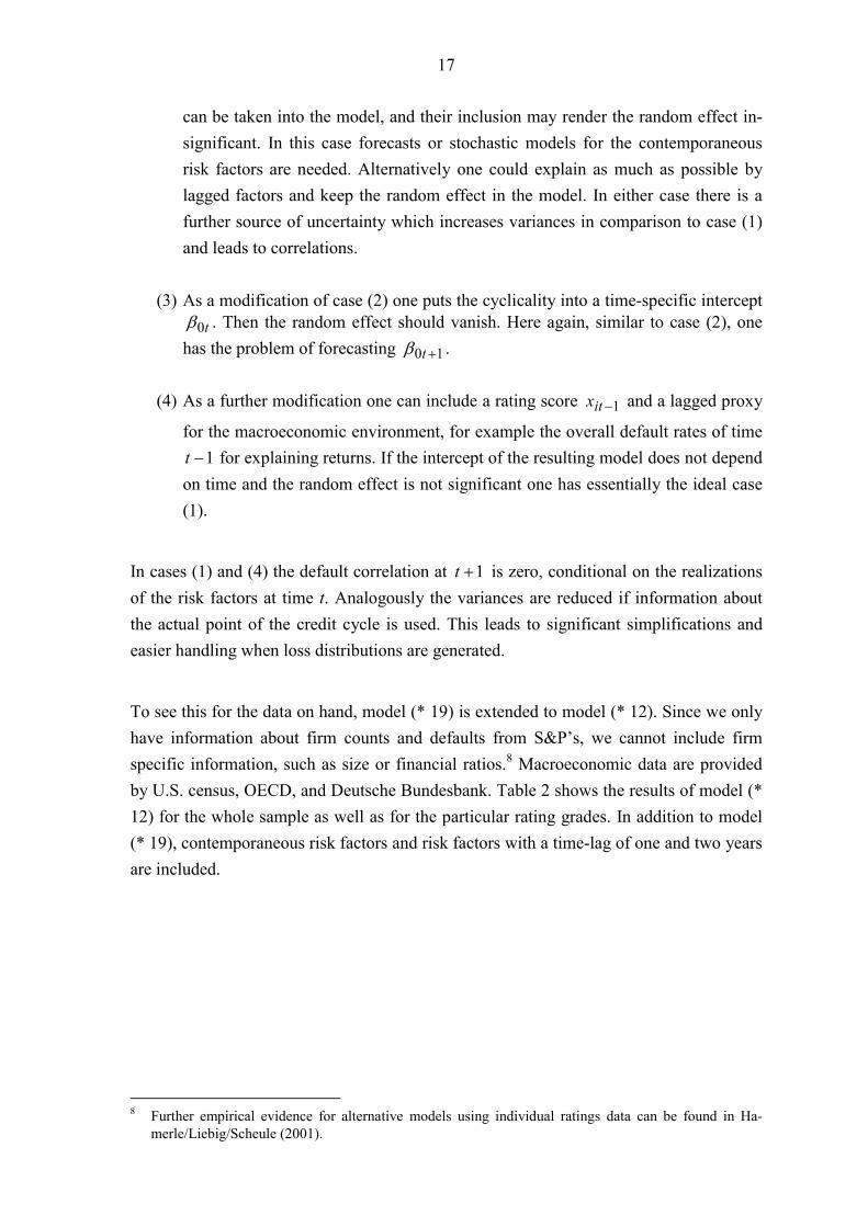
To see this for the data on hand, model (* 19) is extended to model (* 12). Since we onlyhave information about firm counts and defaults from S&P’s, we cannot include firmspecific information, such as size or financial ratios.8 Macroeconomic data are providedby U.S. census, OECD, and Deutsche Bundesbank. Table 2 shows the results of model (*12) for the whole sample as well as for the particular rating grades. In addition to model(* 19), contemporaneous risk factors and risk factors with a time-lag of one and two yearsare included.

8 Further empirical evidence for alternative models using individual ratings data can be found in Ha-

merle/Liebig/Scheule (2001).

18

Table 2: Parameter estimates from model (* 12) with macroeconomic data.

Parameter Estimate Standard Error Pr > |t|

All Grades SQRT(rho) 0.0967 0.02569 0.0017const. -2.2145 0.03461 <.0001DSER_2 0.0980 0.03337 0.0097IND_IP -0.1733 0.03923 0.0004

BB SQRT(rho) 0.0821 0.08969 0.3728const. -2.2529 0.05610 <.0001FEDR_1 0.2319 0.04779 0.0001

B SQRT(rho) 0.0636 0.04410 0.1684const. -1.6025 0.03848 <.0001UNEM_2 -0.0391 0.03655 0.3007DSER_2 0.0753 0.03935 0.0738IND_IP -0.2155 0.04427 0.0002

CCC SQRT(rho) 0.0724 0.1485 0.6321const. -0.8569 0.05653 <0.0001UNEM_1 -0.2749 0.06705 0.0007

IND_IP: Change of Industrial ProductionUNEM: Rate of UnemploymentFEDR: Federal Funds RateDSER: Percentage Change in Real Services Sector Value Added_1: One-year time-lag_2: Two-year time-lag

SQRT(rho) = �

Firstly, from the first rows in Table 2 it can be seen that over all grades two risk factorsare not enough to explain the random effect. We found that an additional variable doesnot lead to a further substantial decrease. However, the random effect variation can bereduced from 0.2 to approximately 0.1, leading to a reduction of asset correlation from4% to approximately 1%. The reduction stems from one lagged variable and one contem-poraneous variable (Change of Industrial Production). Thus, it seems that the whole sam-ple of borrowers is too heterogeneous for being able to be fully explained by only fewrisk factors.

Then, the rating grades are analysed separately. Table 2 shows that we found a few riskfactors which are able to explain the variation of the random effect. In each grade, theeffect is reduced and no longer significantly different from zero. In grade B, altogetherthree factors are needed and one of them is contemporaneous (Change of Industrial Pro-duction). This is an example of case (2). For generating loss distributions this commonfactor has to be forecasted or simulated. Thus, in general correlations remain significant.

19

In grades BB and CCC, however, there is one single factor each, which explains the cor-relation. In addition, this factor drives the default risk with a time lag. These grades areexamples for the ideal case (4) without additional variables needed. Defaults in thesegrades are independent, conditional on the value of the respective risk factor. In gradeBB, an increase of the Federal Funds Rate comes along with an increase of default prob-abilities in the following year. This is reasonable because higher rates may lead to higherinterest rates for debt. In grade CCC, higher unemployment is associated with decreasingdefault probabilities in the next year. This may also be plausible for two reasons. Firstly,if firms take measures for rationalizations they release employees. In the following years,their cost pressures decrease leading to lower default risk. Secondly, the state may stimu-late the economy by higher public expenditures in times of higher unemployment. Thiscould also decrease default risk.

Some comments are in order. The identified factors should be interpreted only as proxiesfor the underlying risk drivers. It is not meant to say, for example, that a higher Fund Rateis virtually responsible for default risk. Furthermore, we do not mean to have completelyidentified the whole risk structure. In banks’ portfolios there may be different structuresthan in the portfolio underlying the S&P data. In addition, only one risk factor may not beenough for explaining correlations. Rather, a rating score or additional variables will haveto be included. Nevertheless, we think that the shown results give first evidence for theappropriateness of a dynamic view of credit risk by model (* 12) and the empirical identi-fication of systematic credit risk factors.

6 Summary and Conclusion

In the new Basel capital accord default probabilities and asset or default correlations arekey factors for determining risk weights under the IRB approach. Modeling and estima-tion of default probabilities and default correlations are central for credit risk modelssince value-at-risk calculations are very sensitive due to changes of these parameters.

The model which is assumed in the Basle Capital Accord starts with given unconditionalPDs and models conditional PDs for a special realization of an unknown risk factor. Itdoes not prescribe how to model these unconditional PDs. The purpose of the presentpaper is to pick up the suggestion of the New Capital Accord and to show how uncondi-tional PDs can be modelled within the Basel II framework. Thus, the Basel II model isextended to an explanatory model for the process which generates asset returns and de-fault probability.

20

It is shown that the latent model for the returns on a firm’s assets is essentially a linearrandom effects panel model. In the case when proxies for asset returns are observable,this linear model can be used. When only defaults are observable, an appropriate thresh-old model leads to a non-linear random effects probit or logit model. The important ad-vantage of the model is that it uses actual information about the point in time of the creditcycle. By this, uncertainties in portfolio Value-at-Risk calculations may be substantiallyreduce. First empirical evidence for the appropriateness of these models and underlyingrisk factors is given with ratings data.

21

References

Altman, E.I, Saunders, A., 1998. Credit Risk Measurement: Developments Over the Last20 Years. Journal of Banking and Finance 21, 1721-1742.

Bank of Italy, 2001. Calibration of Benchmark Risk Weights in the IRB Approach ofRegulatory Capital Requirements, October.

Basel Committee on Banking Supervision, 2003. The New Basel Capital Accord. Con-sultative Document, April.Basel Committee on Banking Supervision,2001. Potential Modifications to the Committee’s Proposals, November.

Basel Committee on Banking Supervision, 2001. The New Basel Capital Accord. Con-sultative Document, January.

Basel Committee on Banking Supervision, 2000. Credit Ratings and ComplementarySources of Credit Quality Information. No 3, August.

Basel Committee on Banking Supervision, 1999b. A New Capital Adequacy Framework.No. 50, June.

Basel Committee on Banking Supervision, 1999a. Credit Risk Modeling: Current Prac-tices and Applications. No. 49, April.

Black, F., Cox, J.C., 1976. Valuing Corporate Securities: Some Effects of Bond IndentureProvisions. Journal of Finance 31, 351-367.

Black, F., Scholes, M., 1973. The Pricing of Options and Corporate Liabilities. Journal ofPolitical Economy, 637-654.

Chen, N.-F., Roll, R., Ross, S.A., 1986. Economic Forces and the Stock Market, Journalof Business 59, p. 383-403.

Collin-Dufresne, P., Goldstein, R.S., Martin, J.S., 2001. The Determinants of CreditSpread Changes. Journal of Finance, Vol. 56, December, 2135-2175.

Connor, G., 1995. The Three Types of Factor Models: A Comparison of Their Explana-tory Power, Financial Analysts Journal, May-June, 42-46.

Credit Suisse Financial Products, 1997. CreditRisk+ - A Credit Risk ManagementFramework. London.

Crosbie, P., 1998. Modeling Default Risk. KMV Corporation, San Francisco.Crouhy, M., Galai, D., Mark, R., 2001. Prototype Risk Rating System. Journal of Bank-

ing and Finance 25, 47-95.Crouhy, M., Galai, D., Mark, R., 2000. A Comparative Analysis of Current Credit Risk

Models. Journal of Banking and Finance 24, 59-117.Duffee, G.R., 1998. The Relationship Between Treasury Yields and Corporate Bond

Yield Spreads. Journal of Finance 53, 2225-2241.Duffie, D., Singleton, K., 1999. Modeling Term Structures of Defaultable Bonds. Review

of Financial Studies 12, 687-720.

22

Duffie, D., Singleton, K.J., 1997. An Econometric Model of the Term Structure of Inter-est-Rate Swap Yields. Journal of Finance 52, 1287-1322.

Efron, B., 1975. The Efficiency of Logistic Regression Compared to Normal Discrimi-nant Analysis. Journal of the American Statistical Association 70, 892-898.

Fama, E.F., French, K.R., 1992. The Cross-Section of Expected Stock Returns. Journal ofFinance 47, 427-465.

Finger, C.C., 2001. The One-Factor CreditMetrics Model in The New Basel Capital Ac-cord. RiskMetrics Journal, Vol. 2(1), 9-18.

Finger, C.C., 1999. Conditional Approaches for CreditMetrics Portfolio Distributions.CreditMetrics Monitor, April, 14-33.

Geske, R., 1977. The Valuation of Corporate Liabilities as Compound Options. Journalof Financial and Quantitative Analysis 12, 541-552.

Gordy, M.B., 2001. A Risk-Factor Model Foundation for Ratings-Based Bank CapitalRules. Board of Governors of the Federal Reserve System. Working Paper.

Gordy, M.B., 2000. A Comparative Anatomy of Credit Risk Models. Journal of Bankingand Finance 24, 119-149

Gordy, M.B., Heitfeld, N., 2000. Estimating Factor Loadings When Ratings PerformanceData Are Scarce. Board of Governors of the Federal Reserve System, Division ofResearch and Statistics, Working Paper.

Gupton, G.M., Finger, C., Bhatia, M., 1997. Credit Metrics - Technical Document.Morgan Guaranty Trust Co., New York.

Hamerle, A., Liebig, T., Scheule, H., 2001. Dynamische Modellierung von Kreditrisikenmit zeitdiskreten Hazardraten. Working Paper, University of Regensburg, Deut-sche Bundesbank.

Hamerle, A., Rösch, D., 2001. Risk Factors and Correlations for Credit Quality Changes.Forthcoming in: Zeitschrift für Betriebswirtschaftliche Forschung (in German).

Hamerle, A., Tutz, G., 1989. Diskrete Modelle zur Analyse von Verweildauern und Le-benszeiten. Frankfurt/Main, New York.

Jarrow, R.A., Turnbull, S.M., 2000. The Intersection of Market and Credit Risk. Journalof Banking and Finance 24, 271-299.

Jarrow, R.A., Lando,D., Turnbull, S.M., 1997. A Markov Model of the Term Structure ofCredit Spreads. Review of Financial Studies 10.

Jarrow, R.A., Turnbull, S.M., 1995. Pricing Derivatives of Financial Securities Subject toCredit Risk. Journal of Finance 50, 53-85.

Kalbfleisch, J.D., Prentice, R.L., 1980. The Statistical Analysis of Failure Time Data.Wiley, New York.

Koyluoglu, H.U., Hickman, A., 1998. A Generalized Framework for Credit Risk PortfolioModels. Working Paper. Oliver, Wyman & Co.http://www.erisk.com/reference/archive/058_183GeneralizedFrameworkd.pdf

23

Lando, D., 1998. On Cox Processes and Credit Risky Securities. Review of DerivativesResearch 2, 99-120.

Lo, A.W., 1985. Logit versus Discriminant Analysis – A Specification Test and Applica-tion to Corporate Bankruptcies. Journal of Econometrics 31, 151-178.

Longstaff, F.A., Schwartz, E.S., 1995. A Simple Approach to Valuing Risky Fixed andFloating Rate Debt. Journal of Finance 50, 789-819.

Lucas, A., Klaassen, P., Spreij, P., Straetmans, S., 2000. An Analytic Approach to CreditRisk of Large Corporate Bond and Loan Portfolios. Working Paper. Forthcomingin: Journal of Banking and Finance.

Madan, D., Unal, H., 1998. Pricing the Risks of Default. Review of Derivatives Re-search 2, 121-160.

Merton, R., 1977. On the Pricing of Contingent Claims and the Modigliani-Miller Theo-rem. Journal of Financial Economics 5, 241-249.

Merton, R., 1974. On the Pricing of Corporate Debt: The Risk Structure of Interest Rates.Journal of Finance 29, 449-470.

Moody’s Investor Service, 1998. Moody’s Credit Ratings and Research. New York.Ong, M.K., 1999. Internal Credit Risk Models – Capital Allocation and Performance

Measurement. Risk Books, London.Pedrosa, M., Roll, R., 2001. Systematic Risk in Corporate Bond Credit Spreads. Journal

of Fixed Income 8, 7-26.Standard & Poor’s, (2001a). Corporate Ratings Criteria. New York.Standard & Poor’s (2001b) Ratings Performance 2000 – Default, Transition, Recovery,

and Spreads. New York.Tutz, G., 2000. Die Analyse kategorialer Daten – eine anwendungsorientierte Einführung

in Logit-Modellierung und kategoriale Regression. München.Wilson, T., 1997a. Portfolio Credit Risk I. Risk, September.Wilson, T., 1997b. Portfolio Credit Risk II. Risk, October.Zhou, C., 2001, An Analysis of Default Correlations and Multiple Defaults, Review of

Financial Studies, Vol. 14, S. 555-576.