Creep and Shrinkage Effects

on Steel-Concrete Composite Beams

Seunghwan Kim

Thesis submitted to the faculty of

the Virginia Polytechnic Institute and State University

in partial fulfillment of the requirements for the degree of

Master of Science

In

Civil Engineering

Roberto T. Leon, Chair

Carin L. Roberts-Wollmann

Zachary Grasley

May 1st, 2014

Blacksburg, Virginia

Keywords: Creep and Shrinkage, Steel-Concrete Composite Beams,

Time-dependent Behaviors, Long-term Deflections

Creep and Shrinkage Effects on Steel-Concrete Composite Beams

Seunghwan Kim

ABSTRACT

Predicting the long-term behavior of steel-concrete composite structures is a very complex

systems problem, both because obtaining reliable information on material properties related to

creep and shrinkage is not straightforward and because it is not easy to clearly determine the

correlation between the effects of creep and shrinkage and the resultant structural response. Slip

occurring at the interface between the steel and concrete may also make prediction more

complicated. While the short-term deflection of composite beams may be easily predicted from

fundamental theories of structural mechanics, calculating the long-term deflection is complicated

by creep and shrinkage effects on the concrete deck varying over time. There are as yet no

comprehensive ways for engineers to reliably deal with these issues, and the development of a

set of justifiable numerical standards and equations for composite structures that goes beyond a

simple commentary is well overdue.

As the first step towards meeting this objective, this research is designed to identify a simple

method for calculating the long-term deformations of steel-concrete composite members based

on existing models to predict concrete creep and shrinkage and to estimate the time-varying

deflection of steel-composite beams for design purposes. A brief reexamination of four existing

models to predict creep and shrinkage was first conducted, after which an analytical approach

using the age-adjusted effective modulus method (AEMM) was used to calculate the long-term

deflection of a simply-supported steel-concrete composite beam. The ACI 209R-92 and CEB

iii

MC90-99 models, which adopt the concept of an ultimate coefficient, formed the basis of the

models developed and examples of the application of the two models are included to provide a

better understanding of the process involved. For the analytical approach using the AEMM, the

entire process of calculating the long-term deflections with respect to both full and partial shear

interactions is presented here, and the accuracy of the calculation validated by comparing the

model predictions with experimental data. Lastly, the way the time-dependent deflection varies

with various combinations of creep coefficient, shrinkage strain, the size of the beam, and the

span length, was analyzed in a parametric study. The results indicate that the long-term

deflection due to creep and shrinkage is generally 1.5 ~ 2.5 times its short-term deflection, and

the effects of shrinkage may contribute much more to the time-dependent deformation than the

effect of creep for cases where the sustained live load is quite small. In addition, the composite

beam with a partial interaction exhibits a larger mid-span deflection for both the short- and long-

term deflections than a beam with a full shear interaction. When it comes to the deflection

limitations, it turned out that although the short-term deflections due to immediate design live

load satisfy the deflection criteria well, its long-term deflections can exceed the deflection

limitations.

iv

Acknowledgement

First of all, I would like to express my special appreciation and thanks to my advisors Professor

Dr. Roberto T. Leon who has been a tremendous mentor for me. I would like to thank him for

encouraging my research and for allowing me to grow as a research scientist. His advice on both

research as well as on my career have been priceless.

I would also like to thank my committee members, Professor Dr. Zachary Grasley and Professor

Dr. Carin L. Roberts-Wollmann for serving as my committee members. I also want to thank you

for letting my defense be an enjoyable moment, and for your comments and suggestions.

A special thanks to my family. Words cannot express how grateful I am to my wife for all of the

sacrifices that she has made on my behalf. Her prayers and support for me were what sustained

me thus far. I would also like to thank all of my friends, especially Hyojoon Bae, Seungmo Kim,

and Jaeeung Kim, who supported me in researching and writing, and incentivized me to strive

towards my goal.

v

Table of Contents

Chapter. 1  Introduction ............................................................................................................... 1 

1.1  Overview of composite structures .................................................................................... 1 

1.2  Methodology .................................................................................................................... 5 

1.3  Organization ..................................................................................................................... 6 

Chapter. 2  Literature review ....................................................................................................... 8 

2.1  Background ...................................................................................................................... 8 

2.2  Creep and shrinkage ......................................................................................................... 9 

2.3  Structural Effects .............................................................................................................11 

2.4  Composite Action ........................................................................................................... 16 

2.5  Shear Studs ..................................................................................................................... 19 

Chapter. 3  Reexamination of the proposed models .................................................................. 22 

3.1  Fundamentals of creep and shrinkage ............................................................................ 22 

3.1.1  General .................................................................................................................... 22 

3.1.2  Brief introduction to the four existing models ........................................................ 27 

3.2  Application of ACI 209R-92 and CEB MC90-99 .......................................................... 35 

3.2.1  Application to an example model ........................................................................... 36 

3.2.2  Summary ................................................................................................................. 40 

3.3  Variable ambient conditions ........................................................................................... 41 

3.3.1  Analysis reflecting variable ambient relative humidity .......................................... 41 

3.3.2  Comparison with experimental data ....................................................................... 45 

3.3.3  Summary ................................................................................................................. 47 

Chapter. 4  Long-term deflection of a simply-supported beam ................................................. 49 

4.1  Age-adjusted Effective Modulus Method (AEMM) ...................................................... 49 

4.2  Deflection of steel-concrete composite beams ............................................................... 51 

4.2.1  Full interaction composite beams ........................................................................... 52 

4.2.2  Partial composite beams ......................................................................................... 59 

4.3  Validation with real experimental data ........................................................................... 68 

vi

4.3.1  Comparison with the test data from Alsamsam (1991) ........................................... 69 

4.3.2  Comparison with the test data of Bradford and Gilbert (1991) .............................. 76 

Chapter. 5  Parametric study...................................................................................................... 81 

5.1  Parameter setting ............................................................................................................ 81 

5.1.1  Concrete properties related to creep and shrinkage ................................................ 82 

5.1.2  Configuration of the composite beams ................................................................... 82 

5.1.3  Other factors............................................................................................................ 83 

5.2  Analysis and results ........................................................................................................ 85 

5.2.1  Short-term deflection due to the immediate design live load ................................. 85 

5.2.2  The ratio of the long-term and short-term deflections due to creep and shrinkage 88 

5.2.3  Comparison with AISC simple model to predict the long-term deflection ............ 94 

Chapter. 6  Conclusions ............................................................................................................. 97 

6.1  Summary of contributions .............................................................................................. 97 

6.2  Research limitations and future work ............................................................................. 99 

References………………………………………………………………………………………101

Appendix A MathCAD routine……………………………………………………………....104

Appendix B Worked out example……………………………………………………………106

vii

List of Figures

Figure 3.1 Creep strain with time ................................................................................................. 23 

Figure 3.2 Drying shrinkage of concrete ...................................................................................... 24 

Figure 3.3 Shrinkage strain comparison ....................................................................................... 37 

Figure 3.4 Creep coefficient comparison ...................................................................................... 38 

Figure 3.5 Total strain comparison ............................................................................................... 40 

Figure 3.6 Influence of the relative humidity in the ACI 209R-92 model .................................... 42 

Figure 3.7 The schematic concept of changes in creep and shrinkage rate depending on the RH 43 

Figure 3.8 Comparison of the effect of variable ambient relative humidity ................................. 44 

Figure 3.9 Cyclic relative humidity (RH=90 40%) (Müller and Pristl, 1993) ........................ 45 

Figure 3.10 Development of shrinkage strain in concrete specimens with diameter of 50mm at variable (RH=90 40%) and constant (RH =65%) ambient humidity (Müller and Pristl, 1993)....................................................................................................................................................... 46 

Figure 3.11 Comparison of the shrinkage strain results predicted by the proposed method with Müller and Pristl’s (1993) experimental data ................................................................................ 46 

Figure 4.1 Gradually reducing stress history ................................................................................ 49 

Figure 4.2 The creep strain and the effective modulus of elasticity ............................................. 50 

Figure 4.3 Deflection and initial strain distribution ...................................................................... 53 

Figure 4.4 Deflection of a simply-supported beam ...................................................................... 55 

Figure 4.5 Instantaneous and time-dependent strain distribution for a steel-concrete cross-section....................................................................................................................................................... 57 

Figure 4.6 (a) Slip of a composite beam, (b) Strain distribution with slip ................................... 60 

Figure 4.7 Shear force developed on the interface and strain distribution with the slip ............... 61 

Figure 4.8 (a) Final strain with the slip, (b) Strain without the slip, (c) Slip strain only .............. 65 

Figure 4.9 The results of typical analyses for partially composite beams .................................... 68 

Figure 4.10 Ambient relative humidity condition ......................................................................... 71 

Figure 4.11 Cross-section and elevation of the beam ................................................................... 71 

Figure 4.12 Creep coefficient and shrinkage strain, using ACI209R-92 ...................................... 74 

Figure 4.13 Comparison of time-dependent deflection for the test data and the proposed method....................................................................................................................................................... 75 

Figure 4.14 Test set up (a) elevation, (b) cross-section, (c) stud .................................................. 77 

viii

Figure 4.15 Comparison of time-dependent deflection for the test data and the proposed method....................................................................................................................................................... 79 

Figure 5.1 A typical steel-concrete composite beam for the analysis ........................................... 82 

Figure 5.2 (a) Loading for the short-term deflection, (b) Loading for the long-term deflection .. 89 

Figure 5.3 Calculation of shrinkage effects .................................................................................. 95 

ix

List of Tables

Table 3.1 Combination of loading, restraining, and humidity conditions .................................... 26 

Table 3.2 Material properties chosen to demonstrate the use of ACI 209R-92 and CEB MC90-99....................................................................................................................................................... 36 

Table 3.3 Comparison of the ultimate shrinkage strain and the creep coefficient ........................ 37 

Table 3.4 The variable relative humidity conditions ..................................................................... 44 

Table 3.5 Specimen properties Müller and Pristl (1993) .............................................................. 45 

Table 4.1 The relationship between the longitudinal force Q and the slip .............................. 64 

Table 4.2 Input variables for the application example .................................................................. 67 

Table 4.3 Construction conditions ................................................................................................ 70 

Table 4.4 Concrete mix variables and curing conditions .............................................................. 70 

Table 4.5 Cross-sectional properties ............................................................................................. 72 

Table 4.6 Loading conditions ........................................................................................................ 72 

Table 4.7 Comparison of instantaneous mid-span deflection ....................................................... 73 

Table 4.8 Comparison of the mid-span deflection 200 days after casting .................................... 75 

Table 4.9 Information on creep and shrinkage .............................................................................. 77 

Table 4.10 Cross-sectional properties ........................................................................................... 77 

Table 4.11 Loading conditions and shear studs ............................................................................ 78 

Table 4.12 Results of the short-term mid-span deflection ............................................................ 79 

Table 4.13 Comparison of the mid-span deflection after 250 days .............................................. 80 

Table 5.1 Concrete properties affecting the structural response ................................................... 82 

Table 5.2 Configuration of the composite beam ........................................................................... 83 

Table 5.3 Effective width according to the span length ................................................................ 83 

Table 5.4 Loading configuration ................................................................................................... 84 

Table 5.5 Full interaction beams; immediate deflection limitation check due to live load .......... 86 

Table 5.6 50% partial interaction beams; immediate deflection limitation check due to live load....................................................................................................................................................... 87 

Table 5.7 25% partial interaction; immediate deflection limitation check due to live load ......... 87 

Table 5.8 Reasonable combinations of the size of steel beams and span length .......................... 88 

Table 5.9 The ratio of the long-term to the short-term deflection for W18x35.............................90

x

Table 5.10 The ratio of the long-term to the short-term deflection for W21x55...........................91

Table 5.11 The ratio of the long-term to the short-term deflection for W27x94...........................92

Table 5.12 Reasonable combinations of the size of steel beams and span length……………….94

Table 5.13 Long-term deflection from AISC simple model and the proposed method for W18x35…………………………………………………………………………………………..95

Table 5.14 Long-term deflection from AISC simple model and the proposed method for W21x55…………………………………………………………………………………………..96

Table 5.15 Long-term deflection from AISC simple model and the proposed method for W27x94…………………………………………………………………………………………..96

1

Chapter. 1 Introduction

1.1 Overview of composite structures

Composite steel-concrete structures have been finding many new applications in building and

bridge construction, generally in the form of Steel Framed Reinforced Concrete Structures (SRC),

Concrete Filled Tube columns (CFTs), and steel-concrete composite beams. This increasing

popularity is largely because these structural elements combine the high tensile strength of steel

with the high compressive strength of concrete. Not only does this type of steel-concrete

composite system provide adequate strength and stiffness in structures, it also brings additional

benefits such as cost-effectiveness in the use of materials, shorter construction times, and better

fire-resistance. Furthermore, recent research into steel-concrete composites has improved the

material’s sustainability profile by replacing much of the Portland cement content, a major

source of CO2 emissions, with less environmentally damaging supplementary cementitious

materials (SCMs) (Gunnarsson et al. 2012).

However, in spite of this composite action’s utility in a structural member, design methods that

employ steel-concrete composite structures require some improvements. Although accurate

models and code provisions are available to determine the strength of composite members, good

methods to predict their short- and long-term deformation behavior, as well as other

serviceability criteria, are lacking. In particular, the long-term analysis of the time-dependent

behavior of composite structures is extremely complicated, requiring consideration of many

unpredictable factors related to both the material itself and the characteristics of the interactions

2

within a composite member (Gilbert and Bradford 1995). Currently the design of steel-concrete

members often either ignores or overestimates the time effects or uses very simplified techniques

such as assuming an arbitrary flexural rigidity (EI) or ultimate creep and shrinkage values. For

this reason, current designs incorporating steel-concrete composite structures generally involve

making estimates, and in many cases engineers’ judgment is needed due to the perceived lack of

useful design guidelines and specifications.

The first issue concerning the use of these composite systems that must be addressed is the level

of uncertainty regarding the material properties of concrete with respect to creep and shrinkage.

The measurement of creep and shrinkage in composite structures is not straightforward because

concrete, a major component, follows a viscoelastic, time-varying behavior. Although a number

of design provisions have been developed to deal with the way both creep and shrinkage change

with time, all these models are simply ways to more closely estimate the real behavior and each

of the design approaches can show divergent results in calculation. Moreover, none of the

approaches based on these design codes accurately reflect actual conditions on construction sites

since most calculations for creep and shrinkage regard ambient conditions, which in real-world

settings will vary considerably, as constant factors in order to simplify the often complex

calculations. Most creep and shrinkage models thus fail to take into account the effects of

fluctuations in relative humidity and temperature.

The second difficulty in analyzing the behavior of composite steel-concrete systems is the

3

structural complexity that inevitably results when two very different materials such as steel and

concrete are combined into a single composite member. As stated above, the composite element

becomes both stiffer and stronger due to the synergistic combination of the structural advantages

that each material brings to the system, and the performance of the resulting composite structure

will thus be better than that of the steel and concrete components acting in isolation in a non-

composite fashion (Johnson and Buckby 1975). However, acting compositely implies that two

materials may be considered to be a single member, and this potentially requires the additional

process of defining new cross-sectional properties and flexural rigidities. At this point, the

problem is that a steel-concrete composite structure is highly likely to change its structural

properties with time, which means that it is very difficult for designers to define the correct

cross-sectional properties and flexural rigidities at every moment when conducting a long-term

analysis. Another aspect of this problem is that steel-concrete composite members generally

undergo changes in their composite action as a result of slip at the interface between the steel and

concrete. The extent of this slip is not only difficult to predict but also often leads to partial

interactions between the composite components, which may have a significant effect on the

analysis compared to the full interaction that would normally be expected (Bradford and Gilbert

1992). This complexity of the composite system derives from the unclear flexural rigidity of the

member and the partial interaction tendency is thus a considerable obstacle when designing steel-

concrete composite structures.

Although it has been generally recognized that long-term analyses of steel-concrete composite

4

structures are hard to accomplish, the fact that many structural engineers continue to place a

major emphasis on this is an indication of the importance of serviceability in the design of

buildings. In structural engineering, both strength and serviceability are considered essential

objectives that all designers must achieve in their design work, and serviceability in particular is

receiving a great deal of attention at present as the development of advanced materials and state

of the art technologies has begun to fulfill the need for greater capacity in structural strength.

Under long-lasting service loads, the ability of buildings to perform safely without deforming,

cracking, and vibrating has become a significant new criterion for measuring the success of

structurally advanced modern buildings. In this context, paying long-overdue attention to the

serviceability of steel-concrete composite structures that may be subject to some, at least, of the

sensitive deformational characteristics of their concrete component is a vital topic for those

seeking to improve the design of structures.

Narrowing the research range down to a consideration of steel-concrete composite beams,

specifically their long-term deflection over time, nonetheless addresses a significant issue

because the ultimate deflection obtained from the long-term analysis may be several times the

instantaneous short-term deflection, with consequently negative effects on the usability of these

composite beams as a building material. The day-to-day deflection thus plays a significant role in

the performance of a steel-concrete beam, but calculating its time-varying deflection is a

convoluted process due to the many variables involved.

5

This research therefore investigates the design issues that affect the performance of the existing

models that are most commonly used to predict concrete creep and shrinkage based on the

concrete properties and various local environmental variables. The time-varying deflection of a

steel-concrete composite beam for design purposes will also be studied using time-dependent

analysis to reveal how creep and shrinkage effects of a concrete deck affect the long-term

deflection of the composite beams of which it is composed.

1.2 Methodology

First, a number of research efforts related to composite beam deflection behavior will be

reviewed. This review will be devoted to both an examination of creep and shrinkage, which are

considered to be a main cause of the time-dependent behavior of steel-concrete composite beams,

as well as to a discussion of analytical approaches to evaluate the resultant structural response

due to creep and shrinkage. Furthermore, past studies on shear interaction mechanism between

steel and concrete will be considered, including the issue of a load-slip relationship in composite

members.

As relevant to this thesis, two topics will be examined. First, a reexamination of the proposed

existing models for predicting creep and shrinkage of concrete, and second, the long-term

deflection of a simply-supported composite beam. For the first topic, fundamental information on

the existing models and application examples will provide basic background, after which the

concept of utilizing variable ambient conditions in predicting creep and shrinkage, seldom

6

included in the existing models, will be proposed. For the second topic, a method to calculate the

mid-span deflection of steel-concrete composite beams is presented with detailed equations,

explaining the contrasting behavior of full versus partial composite beams. At the same time, in

order to validate the reliability of the analytical approach, the research will adopt real

experimental data reported by previous researchers and compare the results from the proposed

method in this thesis with previous test data.

The final step is to do a parametric study about how and how much many variables may affect

the results. Of the wide variety of variables involved, the most frequently-used in construction

utilizing steel-concrete composite beams will be examined, namely the properties of concrete,

structural configuration of the composite beams, and the type of loading.

1.3 Organization

The remainder of this thesis is organized as follows.

Chapter 2 contains a review of the past studies related to the subject of this thesis, and Chapter 3

gives a description of the proposed existing models for predicting creep and shrinkage, in

addition to provide application examples regarding the methods introduced in the models. The

chapter also includes the concept of considering variable relative humidity in predicting creep

and shrinkage. Chapter 4 describes both the analytical approach for calculating the long-term

deflection and its validation using the existing test data. In Chapter 5, a parametric study is

included in order to better assess the effects of many variables resulting in the time-dependent

7

behavior of composite beams. Finally, the thesis concludes by summarizing contributions and

identifying possible future work in Chapter 6.

8

Chapter. 2 Literature review

2.1 Background

Steel-concrete composite frames incorporating normal weight concrete began to be used in the

construction market in the 1920s. However, with a few exceptions, some simple tests with

respect to performance of reinforced cinder-concretes or concrete-encased steel beams

(Christensen 1931; Martin et al. 1930), there was no coordinated fundamental research into their

properties until the 1950s, when Viest and his coworkers began to examine their use in bridges

and other structures (Viest et al. 1958). Simplified design provisions were introduced in the 1961

AISC Specifications (AISC Specification 1961), which along with the commercialization of

shear studs led to a rapid growth of composite floor systems throughout the 1970s and 1980s.

In the tradition of AISC Specifications, little guidance is given to designers as to how to calculate

serviceability criteria, with much of the useful information included in the non-mandatory

commentary. At the time of writing, AISC still does not provide meaningful guidance for

predicting time-dependent behavior of composite structures, while ACI only proposes

prescriptive methods calibrated to older data.

The increasing popularity of these materials in construction therefore makes it imperative that a

more realistic way to calculate the long-term deformation be established, particularly when

considering the importance of the serviceability of buildings which is now a more critical factor

in structural design work than the traditional strength limit state.

A number of previous studies have suggested more accurate ways to analyze the deformation of

9

steel-concrete composite frames and various design codes have been developed that include

useful ways to address design issues for composite members subject to creep and shrinkage.

Researchers have not focused solely on the material properties of concrete itself, particularly

creep and shrinkage, the primary cause of the composite long-term behaviors, but have also

examined the interaction behavior of steel-concrete composite systems and how this depends on

the variable effects of creep and shrinkage. Recent academic interest in composite systems has

extended this into studies of the global behavior of whole structural frames such as multi-span

continuous beams and multi-story buildings, building on the earlier work on the local effects in a

single beam or column due to creep and shrinkage (Varshney et al. 2013).

A closer examination of the literature in this area reveals that most research has been devoted to

one or more of the following issues:

1. material properties of concrete, particularly creep and shrinkage;

2. the time-varying structural response resulting from variable creep and shrinkage;

3. composite action mechanisms, classified as either full or partial interactions; and

4. the contribution of shear connectors and load-slip relationships via push-out experiments.

2.2 Creep and shrinkage

Creep is defined as increase in strain over time under the sustained constant stress, while

shrinkage means decrease in volume with time. In steel-concrete composite structures, creep and

10

shrinkage are highly associated with concrete, and these two inelastic and time-varying strains

cause increase in deformation and redistribution of internal stresses. Therefore, much of the

earlier material research focused on creep and shrinkage. Many useful methods to predict real

behavior more accurately have been suggested, generally supported by extensive experimental

testing to compare the model predictions with real-world data. A number of variables have been

studied for different material properties and various ambient conditions. Trost (1967) and Bazant

(1972) conducted useful studies of creep analysis for concrete structures that led to the

development of a robust method to predict final value of creep, the Age-adjusted Effective

Modulus Method (AEMM) (Bazant 1972; Trost 1967), a more refined version of the Effective

Modulus Method (EMM) (Faber and Jeffcott 1928). While EMM, originally developed by Faber,

was not able to capture change in the effective modulus stemming from the ageing of concrete,

Trost discovered a surprisingly simple way of refining this method to take into account the

reduction in the creep coefficient observed under gradually applied stress. Bazant took this idea

further, presenting a rigorous formulation of the AEMM and extending it to the case of a variable

elastic modulus and an unbounded final value of creep. The inadequacies of the effective

modulus method are to a large extent overcome by the introduction of the ageing coefficient and

this method can be applied for any problem in which strain varies linearly with creep coefficient.

Other researchers have considered the effect of changing ambient conditions corresponding to

the natural climatic variations that structures are exposed to (Bažant and Wang 1985; Hansen

1960; Müller and Pristl 1993). In most practical creep and shrinkage models, no reference is

11

made to the influence of variable environmental conditions. If it is considered, overly simplified

techniques such as arbitrarily introducing average values during the corresponding time period

are applied. Bažant and Wang (1985) and Müller and Pristl (1993) both reported that cyclic

variations of environmental relative humidity can have an remarkable effect on the long-term

deformations of concrete structures, and fluctuations in the ambient relative humidity can also

significantly affect creep and shrinkage. Laboratory measurements on test cylinders revealed that

creep of a specimen exposed to cyclic humidity may be accelerated compared to the creep of an

identical specimen exposed to a constant humidity equal to the same average humidity, whereas

measurements of shrinkage under cyclic humidity revealed no systematic difference from

shrinkage at a constant average humidity (Bažant & Wang, 1985). The creep prediction formulas

of the BP Model can be easily generalized to approximately take into account the increase of

creep caused by the cyclic component of environmental humidity (Müller & Pristl, 1993).

2.3 Structural Effects

Numerous experiments have been undertaken to quantify changes in strain due to creep and

shrinkage for particular scenarios. For example, Bawa (1990) measured construction loads and

the resultant strain variations in creep and shrinkage on the large composite columns making up

the main structural system for a 57-story building during a real-world construction project in

order to track the structural response of composite columns during construction ahead of the

additional service loads that would be applied once the building was handed over. Gunnarsson

and coworkers (2012) studied differences in the creep and shrinkage behavior of CFT columns

12

filled with either conventional self-consolidating concrete or SCM concrete in their investigation

of the performance of CFTs filled with SCMs. The results from their long-term tests were

compared to four existing models for creep and shrinkage to determine if these models provided

acceptable predictions for the long-term behavior of structural CFT components. Their findings

revealed that while some models could lead to quite reliable prediction in some cases, other

models produced comparatively inferior results (Gunnarsson et al. 2012).

The time-dependent effects of creep and shrinkage in concrete may have unfortunate results,

leading to the cracking of concrete, redistribution of moments, creep buckling, and significant

changes in deflections, all of which can change the structural response of composite columns or

beams considerably. A great deal of research has therefore been devoted to identifying

correlations between the effects of creep and shrinkage and the resulting structural behavior in

composite structures. Early research into the structural response in composite structures due to

creep and shrinkage was focused on reinforced concrete structures. Branson and Metz (1963)

studied resisting tensile stresses and cracks in concrete due to bond between concrete and

reinforcing steel, which in some cases leads to a gradual decrease in the moment of inertia of

reinforced concrete beams. They developed an effective moment of inertia expression

empirically based on the test results of simply-supported rectangular reinforced concrete beams.

The method proposed by Branson and Metz was later adopted by ACI 1966 for predicting the

instantaneous deflection of concrete beams. Bresler and Selna (1964), Corley and Sozen (1966),

and Scanlon and Murray (1974) all developed methods to determine the time-dependent

13

deformation of reinforced concrete beams or slabs, taking into account the effects of creep,

shrinkage, and cracking. Bresler and Selna (1964) discussed the principal variables affecting

time-dependent behavior of reinforced concrete structures and described a simplified method for

analysis of stresses and deformation. Corley and Sozen (1966) proposed a simple method for

estimating the time-dependent deflections of reinforced concrete beams based on their

experimental observations of the deformations of four beams over a period of 2 years. Scanlon

and Murray (1974) took a different approach, utilizing finite element analysis to determine the

long-term deflections of reinforced concrete beams. Their analysis employed a rectangular plate

bending element, and applied a numerical time integration approach to evaluate creep and

shrinkage strains determined from CEB parameters, with the model predictions being compared

with experimental results from previous studies.

Alsamsam (1991) dealt with the issue of short- and long-term deflections of composite floor

systems in a wide variety of ways, providing an assessment of the serviceability criteria with

particular emphasis on allowable deflections based on the observation that the LRFD

Specification then in force did not include any specific provisions for serviceability limit states

concerning deflection, cracking, and vibration for composite floor systems. In order to develop

guidelines to mitigate these serviceability problems, Alsamsam began by introducing an

analytical tool for composite floor systems for instantaneous and time-dependent deflections that

accounted explicitly for the effect of shear connection flexibility, concrete slab differential

shrinkage, and creep effects due to sustained loads. The analysis was then verified by comparing

14

the results obtained with the findings of a full-scale experimental testing program in which four

full-scale 32 ft simply supported composite beam specimens with a full interaction between steel

and concrete were built and their time-dependent behavior recorded for a period of 3~6 months

under variable environmental conditions. Alsamsam’s findings confirmed that time-dependent

deflections of a composite beam due to creep and shrinkage are significant and cannot be ignored

during design, highlighting the need for the designer to adequately control both deflection and

cracking at any location or over any time period.

A substantial study of the effects of creep and shrinkage on steel-concrete composite beams was

conducted by Bradford and Gilbert (1991) in the early 1990s. They came up with a number of

analytical approaches that could be used to calculate the short- and long-term strains and

deflections of composite beams. These studies included many design applications and their

findings were supported by useful experimental verifications. For a time-dependent analysis, it is

essential that effects of creep and shrinkage are adequately considered in design because the

force and moment generated in the steel elements of the cross-section by restraining creep and

shrinkage in the concrete result in increased curvature and a gradual transfer of stress from the

concrete to the steel. In most of their published work, Bradford and Gilbert applied existing

methods to deal with the structural response due to creep and shrinkage, such as the Rate of

Creep Method (RCM) and the Age-adjusted Effective Modulus Method (AEMM). Both of these

methods involve solution procedures that ensure compatibility of strains and curvatures at every

point on the cross section, allowing the time-varying stresses and deflection of steel-concrete

15

beams to be obtained (Bradford 1991; Ian Gilbert 1989). Lawther and Gilbert (1992) also

adopted the Rate of Creep Method to analyze the deflection of statically determinate composite

steel-concrete members, utilizing Dischinger’s differential constitutive relationship and stiffness

matrix analysis to model the inelastic creep and shrinkage strains that develop with time in

concrete. In 1991, Bradford and Gilbert reported a significant experimental test to validate their

proposed method with respect to the time-dependent behaviors of composite beams. Four

simply-supported steel-concrete beams were set up and stresses and deformations with time were

monitored for a period of 250 days under the same ambient conditions. The study included push-

out tests to determine the contribution of shear connectors mounted between the steel and

concrete, as well as a comparison of two different connector densities to identify the effect of slip

deformations. The results of this study provided benchmark data for the calibration of theoretical

treatments that incorporate creep, shrinkage, and connector slip (Bradford and Gilbert 1991).

Current research on the long-term behavior of steel-concrete structures associated with creep and

shrinkage is not merely limited to the local behavior of a single composite beam or column. A

more extensive and comprehensive study of the structural response of an entire framework

composed of a number of composite members is now the focus of attention after moving through

an intermediate stage in which engineers extended their research scope into multi-span

composite beams (Gilbert and Bradford 1995). Recent research by Varshney and coworkers

(2013) looked at a wide variety of factors related to the control of time-dependent effects. In their

study, two frames, a single story five bay frame and a five story frame with five spans, were

16

considered for both shored and unshored constructions and an analytical hybrid procedure

designed to account for creep, shrinkage, and progressive cracking in concrete slab panels was

developed. The main focus of this research was the initiating time of mobilization of composite

action between pre-cast concrete and steel, which may eventually result in variations in bending

moments and mid-span deflections. The research team found that the long-term deformations

could be controlled by simply delaying the time of mobilization, the process of assembling and

bond by shear connectors between two different materials. Even though the study’s primary

research focus was on the mobilization of steel and concrete, the data obtained included useful

information of the changes in strains, stresses, and deflections with time in large-scale composite

frames and these data are likely to play a significant role in future research into steel-concrete

composite structures(Varshney et al. 2013).

2.4 Composite Action

Most of the above research related to time-dependent behaviors of steel-concrete composite

beams tends to assume that a perfect composite action between a steel beam and a concrete deck

is maintained under sustained service loads. However, in reality slip deformations will occur at

the interface and consequently the steel and concrete cross section will generally behave

separately in a non-composite manner to some degree, the so-called the partial interaction of

composite beams. A great deal of attention has been paid to this partial interaction problem since

the slip effect not only reduces internal resistant moment and the section modulus in the section

but also increases the internal stress experienced compared with the no-slip case. In the course of

17

their research, Bradford and Gilbert (1991) looked at composite beams with a partial interaction,

building on their preceding research concerning the analysis of steel-concrete composite

structures with full interaction. While examining the time-dependent results due to creep and

shrinkage by means of the experiments on four composite beams described above, they observed

that beams experiencing slip along a slab-steel interface containing a relatively small number of

shear studs had larger values of deflection than similar beams without such slip. Two beams were

designed to have nearly full interaction, with pairs of shear studs at 200mm intervals along the

beam, while the other two beams were designed with pairs of studs at 600mm intervals, allowing

substantial slip to take place between the steel and concrete. Bradford and Gilbert (1992)

developed a theoretical model for the time-dependent response of simply supported composite

beams that combined cross-sectional analysis using the AEMM with longitudinal analysis to take

the slip effects into account. They compared the theory’s predictions with the test results and

found good agreement between the two.

Wang (1998) proposed a shear connector stiffness based approach to deal with the deflection of

steel-concrete composite beams with partial shear interaction. Here, the predicted maximum

beam deflection using the approach was compared against the results from a linear-elastic finite-

element analysis and an existing test on composite beams. In the absence of a reliable way to

calculate the shear connector stiffness, Wang suggested a simple procedure for obtaining the final

deflection. Faella and coworkers (2001) proposed a displacement-based finite-element model for

the analysis of steel-concrete composite beams with flexible shear connections in which the

18

stiffness matrix and the fixed-end nodal force vector were directly derived from the exact

solution of Newmark’s differential equation. The exact approach includes the formulation of the

stiffness matrix K and the vector of equivalent nodal forces Q without the loss of accuracy

introduced by the usual finite models, which assume approximate shape functions for the

displacement field. The analytical expressions of the K and Q terms can be easily integrated into

a finite element computer program as the researchers demonstrated for several cases involving

typical service conditions for steel-concrete composite beams (Faella et al. 2002). In a study of

the accuracy and reliability of various composite cross-sectional analyses introduced in the

present design codes, Nie and Cai (2003) focused on the design specifications that have adopted

the transformed cross-section method for the analysis of composite beams, particularly the AISC

specifications in which the calculating procedure for stress and deflection of partially composite

girders is specified. After presenting the equivalent flexural rigidity concept, including the

effective section modulus and moment of inertia when composite beams are subject to shear slip

effects, they derived a process based on the fundamental equilibrium and curvature compatibility

and then compared the predicted results with experimental measurements of six specimens in

their own lab and those reported previously by other researchers. They concluded that including

slip effects may result in a reduction in stiffness of up to 17% for short span beams, which means

that predictions should indeed take into account slip effects to improve the accuracy of

calculations. Noting that the existing design specifications ignore slip effects in many cases, Nie

and Cai pointed out that those AISC specifications that do take into account slip effects tend to

generate conservative predictions for partial composite sections, in contrast to the fully

justifiable predictions for full composite sections in the AISC specifications.

19

2.5 Shear Studs

A considerable portion of the above research on the structurally different behavior resulting from

full and partial composite interaction involves the use of push-out tests to estimate the flexible

shear strength of stud connectors. This is because in addition to being a good way to test the level

of composite action that can be achieved by the use of shear connectors embedded into concrete,

push-out tests also provide detailed information on the correlation between the types and

numbers of stud connectors and the degree of composite action. The first studies on shear

connectors were undertaken by Viest (1956), who tested full scale load-slip specimens with

various size and spacings of the studs between a steel I-beam and a concrete floor. Round steel

studs were used to determine the behavior and load carrying capacity of stud shear connectors to

confirm that a steel stud is suitable for use as a shear connector in composite concrete and steel

construction. Empirical equations were also presented for determining the critical load. A series

of beam and push-out tests were reported by Slutter and Driscoll (1963), who identified a

functional relationship between connector shear strength and the compressive strength of

normal-weight concrete, enabling information on the ultimate strength of various types of

mechanical shear connectors to be used to develop criteria for minimum shear connector

requirements for composite building members. A method of determining the ultimate strength of

members with shear connectors was developed and applied to the analysis of test results, leading

to recommendations regarding specific values for the minimum number of shear connectors

required for design purposes.

20

Ollgaard et al. (1971) also carried out meaningful research on the load-slip relationship in

composite members using push-out tests. Here, the tests were used to determine the strength and

behavior of connectors embedded in both normal-weight and lightweight concretes so that design

recommendations could be made. The test was developed after the controlled variables were

selected, and the variables considered included the basic material properties, the stud diameter,

type of aggregate, and number of connectors per slab. Forty-eight push-out specimens were

tested during this experiment, consisting of groups of two slab specimens with three specimens

in each group; sixteen cylinders that had been moist-cured for 5 to 7 days were cast for each

group of specimens. Testing was conducted on the 28th day after casting and loads were in 10-kip

increments using a 300-kip capacity hydraulic testing machine. Based on the test results, the

research team concluded that the shear strength of stud connectors embedded in normal-weight

and lightweight concrete was primarily influenced by the compressive strength and the modulus

of elasticity of the concrete and described both an empirically exact function and a simplified

equation for design purposes. They also found that the inclusion of other concrete properties

including the concrete tensile strength and density, did not significantly improve the fit to the test

data and that the shear strength was approximately proportional to the cross-sectional area of the

studs.

To sum up, this review of previous research into the behaviors and analyses of steel-concrete

composite structures due to creep and shrinkage identified four main issues: concrete properties

21

regarding creep and shrinkage, the time-dependent structural response, full and partial interaction

problems, and the load-slip relationship. As a result, the current study will address these

important factors in detail, focusing particularly on the time-varying deflection of steel-concrete

composite beams, in order to better assess the ability of the proposed design provisions to predict

the long-term deflection of composite beams.

22

Chapter. 3 Reexamination of the proposed models

3.1 Fundamentals of creep and shrinkage

3.1.1 General

Creep is the time-dependent increase in strain under a sustained constant load typical of materials

such as concrete that exhibit a time-dependent viscoelastic behavior. It occurs because after the

initial strain induced by an immediate load, the strain experienced by concrete tends to gradually

increase without an additional load being applied. This is primarily due to the hydration

processes in the cement paste and it is highly dependent on the concrete properties, exposure

time, ambient temperature, and the applied structural load. In general, the total strain refers to the

total change in length per unit length of a concrete specimen due to a sustained load under

conditions of 100% ambient humidity and includes both the elastic strain and the creep strain.

A significant characteristic of creep behavior is that the total strain acting on the sample is not

restored to the initial dimension even if the loads that have led to the increase in strain are

removed. Figure 3.1 illustrates how creep strain changes with time, specifically the gradual

increase and decrease in strain depending on time and loading condition. The process is not fully

reversible and thus creep recovery is not complete. Even after the load on the concrete has been

completely removed, permanent and irreversible creep strain remains, although the elastic strain

is recovered.

23

Figure 3.1 Creep strain with time

(From Mindess and Young, Concrete, McGraw-Hill, 1981 and used under fair use, 2014)

Concrete also exhibits another common viscoelastic response known as stress relaxation. When a

load is applied, an instantaneous elastic stress is generated in the concrete specimen that tends to

decrease over time if the initial elastic strain is maintained. This is referred to as stress relaxation.

These two viscoelastic phenomena, creep and stress relaxation, are significant material properties

of concrete, so special attention must be paid to these behaviors in the analysis and design of

concrete structures.

Shrinkage is defined as the decrease in length or volume of an unloaded concrete specimen over

time. The movement of moisture in the hydrated cement paste is the main cause of shrinkage,

which in concrete is generally classified into one of three types. Drying shrinkage, originating

24

from the loss of water from evaporation, makes the largest contribution to shrinkage, but both

thermal shrinkage and carbonation shrinkage play significant roles in the shrinkage process.

Unlike creep, which is affected by the application and removal of loads, shrinkage is closely

linked to the ambient conditions of drying and rewetting. The length or volume of the concrete

specimen decreases during drying, but once the concrete is rewet, the diminished volume

increases again. At this point, the drying shrinkage shows signs of irreversibility, just as creep

behavior does, which means the concrete volume does not return to the original dimension on

rewetting. Figure 3.2 demonstrates the typical shrinkage behavior of concrete.

Figure 3.2 Drying shrinkage of concrete

(From Mindess and Young, Concrete, McGraw-Hill, 1981 and used under fair use, 2014)

Creep, shrinkage, and stress relaxation are all very important factors that must be taken into

account when carrying out analyses of concrete structures since they can lead to significant

redistributions of the internal stresses and, consequently, potentially undesirable increases in the

25

strain and stress experienced by the structures over time. As a result, concrete structures have a

high probability of exhibiting differences in their structural response between their short-term

and long-term behavior due to these time-dependent characteristics of concrete. In practice,

drying shrinkage and the two viscoelastic phenomena, creep and relaxation, usually take place

simultaneously, and various boundary conditions of structures also generate restraining effects in

a different manner. The combined effect of the many possible combinations of loading,

viscoelastic behaviors, and restraining effects bring about structurally divergent responses in a

complex way, as summarized in Table 3.1.

26

Table 3.1 Combination of loading, restraining, and humidity conditions

(From Metha and Monterio, Concrete, McGraw-Hill, 2006 and used under fair use, 2014)

27

3.1.2 Brief introduction to the four existing models

Over the past few decades, several models have been proposed for predicting drying shrinkage,

creep, and total strain in a concrete structure, with the main objective being accuracy and

convenience. Since creep and shrinkage of concrete are too complicated to capture in any detail,

many researchers have instead chosen to propose procedures that approximate the real

phenomena but utilize more convenient methods to facilitate the design process. In this section,

four existing models to predict creep and shrinkage that are in widespread use will be introduced,

and the characteristics of each will be briefly described. The four methods are: ACI 209R-92

(ACI Committee 209 Reapproved 2008), CEB MC90-99 (Muller and Hillsdorf 1990; CEB 1991,

1993, 1999), Bažant-Baweja B3 (Bažant and Baweja 1995, 2000), and GL2000 (Gardner and

Lockman 2001).

1) ACI 209R-92

This empirical model was developed by Branson and Christiason (1971) for use with

precast/prestressed structures and has been used by designers for many decades because the

equations are relatively simple for their purposes. In particular, ACI 209R-08 (ACI Committee

209 Reapproved 2008) is relatively easy to adjust to match short-term test data by modifying the

ultimate shrinkage strain or creep, but it cannot capture creep or shrinkage phenomena exactly

due to its empirical approach. This method is known to have a tendency to overestimate

measured shrinkage at low shrinkage values and underestimate them at high shrinkage values.

28

The design approach includes standard conditions and correction factors to fit non-standard

conditions that are applied to ultimate values.

The ACI 209R-92 creep model is given by:

0.6

00 0.6

0

( , )10

u

t tt t

t t

(3-1)

where 0( , )t t is the creep coefficient at concrete age t due to a load applied at the age to; (t – to)

is the time since application of load, and u is the ultimate creep coefficient. For standard

conditions, the average value proposed for the ultimate creep coefficient u is 2.35. For

conditions other than the standard conditions, u needs to be modified by multiplying it by six

correction factors.

, , , , , ,2.35ou c t c RH c vs c s c sh (3-2)

where , 0c t is a factor taking into account the age of loading; ,c RH is the relative ambient

humidity factor; ,c vs is a factor for the volume-to-surface area ratio; ,c s is a slump factor;

,c is a factor for the ratio of fine aggregate to total aggregate ratio by weight; and ,sh is an air

content factor. These correction factors mostly exhibit almost linear relationship with the

associated variables, and details of each factor can be found in ACI 209R-92 (ACI Committee

209 Reapproved 2008, Appendix A.1). The compliance function, the total load-induced strain

29

(elastic strain plus creep strain) at age t per unit stress, is given by:

00

0

1 ( , ),

cmt

t tJ t t

E

(3-3)

where Ecmto is the modulus of elasticity at the time of loading to.

The shrinkage strain ,sh ct t at age of concrete t (days), measured from the start of

drying at tc (days), is calculated by:

, csh c shu

c

t tt t

f t t

(3-4)

where f takes the value 35 for 7 days of moist curing and 55 for 1 to 3 days of steam curing, for

example. The ultimate shrinkage strain shu is 6780 10 / ( . / .)mm mm in in for the standard

conditions, in the absence of specific shrinkage data for local aggregates and conditions and at an

ambient relative humidity of 40%.

The average value of the ultimate shrinkage strain shu for non-standard conditions can

also be obtained by multiplying it by a series of correction factors.

6, , , , , , ,(780 10 )

cshu sh t sh RH sh vs sh s sh sh c sh (3-5)

Here, the seven correction factors account for the initial moist curing condition ( , csh t ), the

ambient relative humidity ( ,sh RH ), the volume-surface ratio ( ,sh vs ), the slump factor ( ,sh s ), the

ratio of fine aggregate to total aggregate by weight ( ,sh ), the cement content factor ( ,sh c ), and

30

the air content ( ,sh ) in the order shown.

2) CEB MC90-99

CEB MC 90-99 is the more recent version of CEB MC90, a European creep and shrinkage

model initially presented by CEB in 1990 based on the research of Muller and Hillsdorf (Muller

and Hillsdorf 1990; CEB 1991, 1993, 1999). It was updated in 1998 in order to account for

normal- and high-strength concrete and autogenous shrinkage. CEB MC90-99 has a similar

approach to ACI 209R-92 in that both models adopt an ultimate value combined with a series of

modification factors that depend on the properties of the concrete and environmental conditions.

However, unlike ACI 209R-92, CEB MC90-99 does not include any information related to the

type and duration of curing, but instead takes into account the average relative humidity and

member size. For the CEB MC90-99 compliance function, the total strain per unit stress, is

expressed by:

28 00

0 28

,1,

cmt cmt

t tJ t t

E E

(3-6)

where Ecmto and 28cmtE are the modulus of elasticity at the time of loading to and at 28 days,

respectively; 28 0,t t is the 28-day creep coefficient, which may be calculated as the notional

creep coefficient 0 and the developing function with time 0c t t :

28 0 0 0, ct t t t (3-7)

The notional creep coefficient 0 and the developing function with time 0c t t are

31

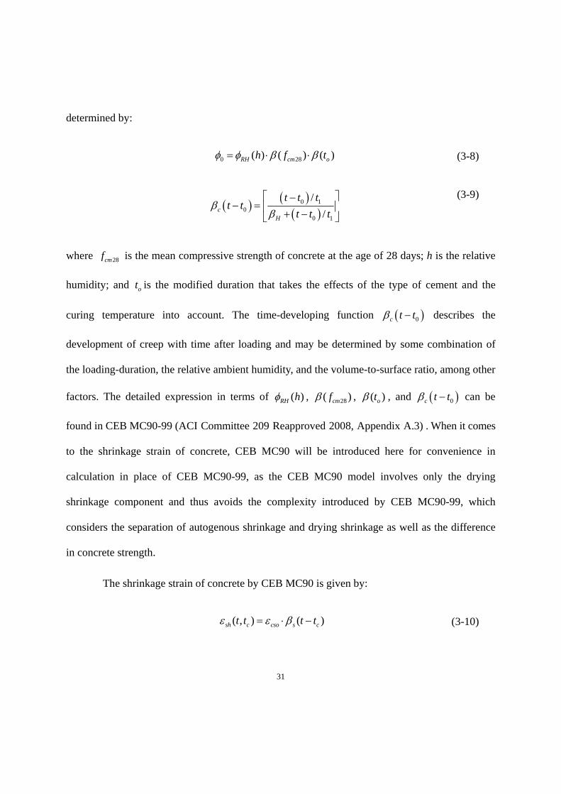
determined by:

0 28( ) ( ) ( )RH cm oh f t (3-8)

0 1

00 1

/

/cH

t t tt t

t t t

(3-9)

where 28cmf is the mean compressive strength of concrete at the age of 28 days; h is the relative

humidity; and ot is the modified duration that takes the effects of the type of cement and the

curing temperature into account. The time-developing function 0c t t describes the

development of creep with time after loading and may be determined by some combination of

the loading-duration, the relative ambient humidity, and the volume-to-surface ratio, among other

factors. The detailed expression in terms of ( )RH h , 28( )cmf , ( )ot , and 0c t t can be

found in CEB MC90-99 (ACI Committee 209 Reapproved 2008, Appendix A.3) . When it comes

to the shrinkage strain of concrete, CEB MC90 will be introduced here for convenience in

calculation in place of CEB MC90-99, as the CEB MC90 model involves only the drying

shrinkage component and thus avoids the complexity introduced by CEB MC90-99, which

considers the separation of autogenous shrinkage and drying shrinkage as well as the difference

in concrete strength.

The shrinkage strain of concrete by CEB MC90 is given by:

( , ) ( )sh c cso s ct t t t (3-10)

32

where cso is the notional shrinkage coefficient, ( )s ct t is the coefficient describing the

development of shrinkage with time of drying, and tc is the age of concrete at the beginning of

drying (days). The notional shrinkage coefficient and the time-developing expressions are

calculated by:

28( )cso s cm RHf (3-11)

with 628

280

( ) 160 10 (9 ) 10cms cm sc

cm

ff

f

(3-12)

3

1.55 1RHo

h

h

(3-13)

0.5

12

0 1

( ) /( )

350 ( ) /( ) ( ) /c

s cV V

S S c

t t tt t

t t t

(3-14)

where 28cmf is the mean compressive cylinder strength of concrete at the age of 28 days; 0cmf is

equal to 10 MPa (1450 psi), sc is a coefficient that depends on the type of cement; h is the

ambient relative humidity as a decimal quantity, with ho equal to 1; and VS is the volume-to-

surface ratio.

3) Bažant-Baweja B3 model

The Bažant-Baweja B3 model is the latest of a series of creep and shrinkage prediction methods

by Bazant and his collaborators (Bazant and Baweja 2000) and is based on a mathematical

33

description of a variety of phenomena affecting creep and shrinkage. It is theoretically better

justified than either of the previous models, but the prediction process is relatively complicated

since this model takes many interacting factors into consideration simultaneously. The

compliance function is composed of the instantaneous strain, the basic creep function, and the

drying creep function, and is calculated by:

0 0 0 0, 1 , , ,d cJ t t q C t t C t t t (3-15)

with the instantaneous compliance,

0

11q

E (3-16)

for basic creep, ( , ) 2 ( , ) 3ln[1 ( ) ] 4 ln( / )o o o o oC t t q Q t t q t t q t t (3-17)

for drying creep, 1/ 2

0 0, , 5 exp 8 exp 8d cC t t t q H t H t (3-18)

where 1q is the instantaneous complicance; q2 is the aging viscoelastic compliance term; q3 is

the nonaging viscoelastic compliance term; q4 is the aging flow parameter; q5 is the drying creep

parameter. The other terms are introduced in the Bažant-Baweja B3 model in more detail (Bažant

and Baweja 1995, 2000).

The shrinkage strain, measured from the start of drying at tc (days), is given by:

( , ) ( )sh c sh h ct t k S t t (3-19)

where sh is the ultimate shrinkage strain; hk is the humidity dependence factor; and

( )cS t t is a time-dependent term. The ultimate shrinkage strain and the time function for

34

shrinkage are calculated by:

607

( )cm

sh scm c sh

E

E t

(3-20)

( )( ) tanh c

csh

t tS t t

(3-21)

The constant, s , and the shrinkage half-time in days, sh , are specifically introduced in the

Bažant-Baweja B3 model.

4) GL 2000

The GL2000 model was proposed by Gardner, who based his new model on the Atlanta 97

model, which was itself influenced by CEB MC-90. According to Gardner and Lockman (2001),

the method can be applied to all kinds of chemical admixtures, casting temperatures, and curing

durations.

The compliance function is given by:

28 0

0 28

,1( , )o

cmt cmt

t tJ t t

E E

(3-22)

where the28-day creep coefficient is:

35

0.5 0.50.3

0.3

0.5

22

( ) ( )7( , ) ( ) 2

( ) 14 ( ) 7

( ) 2.5(1 1.086 )

( ) 77( )

o oo c

o o o

o

VSo

t t t tt t t

t t t t t

t th

t t

(3-23)

where ( )ct is the correction term for the effect of drying before loading and is discussed in

some detail in the GL 2000 model (Gardner and Lockman 2001).

The shrinkage strain of GL 2000 is calculated by:

( , ) ( ) ( )sh c shu ct t h t t (3-24)

where shu is the ultimate shrinkage strain, ( )h is a correction term for the effect of humidity,

and ( )ct t is a correction term for the effect of time of drying.

3.2 Application of ACI 209R-92 and CEB MC90-99

In this section, ACI 209R-92 and CEB MC90-99 will be examined as examples of the

application of creep and shrinkage models, These two models take a similar approach to predict

the final results in that both ACI 209R-92 and CEB MC90-99 adopt the ultimate values for creep

and shrinkage and then apply a modification procedure to reflect various material and

environmental conditions. In addition, the two methods are relatively convenient for simple

predictions of creep and shrinkage values.

36

3.2.1 Application to an example model

To demonstrate the use of ACI 209R-92 and CEB MC90-99, the concrete properties, ambient

conditions, and loadings listed in Table 3.2 will be used. Not all characteristics of the model

system selected are handled well by ACI 209R-92 and CEB MC90-99, and significant variations

in the results will be seen depending on the changes in the variables included. However, the

variables chosen here, specifically the 28-day concrete compressive strength, the cross-sectional

properties of the concrete, and the curing conditions, can be regarded as typical properties of

concrete for steel-concrete composite beams of the type that are the primary focus of this

research.

Table 3.2 Material properties chosen to demonstrate the use of ACI 209R-92 and CEB MC90-99

Concrete properties

28-day compressive strength, f’c = 4 ksi

Modulus of elasticity, Ec = 3,492 ksi

Normal hardening cement

Cross-sectional properties Size of cross-section = (4 in. × 96 in.)

Curing condition 7-day moist-cured

Ambient relative humidity = 60%

Loading condition Sustained stress of (0.3×f’c)

Loaded at 14 days after casting

The ultimate shrinkage value and the creep coefficient were obtained by MathCAD, based on

ACI 209R-92 and CEB MC90-99, and are shown in Table 1.3.

37

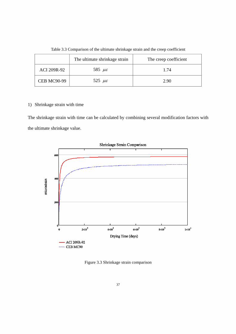
Table 3.3 Comparison of the ultimate shrinkage strain and the creep coefficient

The ultimate shrinkage strain The creep coefficient

ACI 209R-92 585 1.74

CEB MC90-99 525 2.90

1) Shrinkage strain with time

The shrinkage strain with time can be calculated by combining several modification factors with

the ultimate shrinkage value.

Figure 3.3 Shrinkage strain comparison

38

As shown in Figure 3.3, the shrinkage strain rapidly increases at the beginning of the aging

process and then the increase gradually slows with time. In this example model, the ACI 209R-

92 model yields a higher value for the shrinkage strain compared to the result from CEB MC90,

and the rate of shrinkage development obtained using ACI 209R-92 is quicker than that from

CEB MC90.

2) Creep coefficient with time

Creep coefficient over a period of 10,000 days is easily calculated by the two models. As Figure

3.4 demonstrates, ACI 209R-92 results in a significantly lower creep coefficient with time.

Figure 3.4 Creep coefficient comparison

39

3) The total strain with time

The total strain of a concrete specimen is determined by two components: the compliance

function, including the initial elastic strain at the age of loading, and the shrinkage strain with

time, as illustrated in Figure 3.5.

Total strain = (compliance × sustained stress) + shrinkage strain

with (elastic strain + creep )

compliance=stress

0( ) ( , ) ( , )total o shrinkage ct J t t t t (3-25)

where 0 is the sustained stress at the age of loading; ( , )oJ t t is compliance function;

( , )shrinkage ct t is the shrinkage strain with time.

40

Figure 3.5 Total strain comparison

3.2.2 Summary

Utilizing a practical example of the use of two models, ACI 209R-92 and CEB MC90-99, a brief

discussion of creep and shrinkage was presented in this section. A comparison of the

performance of the two models with respect to prediction in creep and shrinkage revealed that in

accordance with the commentary in ACI 209R-92 (ACI Committee 209 Reapproved 2008),

CEB MC90-99 underestimates the shrinkage,

the ACI 209R-92 method underestimates compliance for most real experimental data, and

Overall, however, the prediction results obtained for the example model show good

agreement with the performance assessments provided in ACI 209R-92.

41

3.3 Variable ambient conditions

Although a number of design provisions have been developed to improve the accuracy of creep

and shrinkage predictions with time, those approaches based on the design codes are not able to

realistically reflect the real-world climatic variations on construction sites. This is because most

calculations tend to assume that the ambient conditions affecting creep and shrinkage effects are

constant throughout the calculation period, which is far from the case. Environmental conditions

such as relative humidity (RH) and temperature fluctuate considerably over the course of the day

and from season to season, but none of the creep and shrinkage prediction models make any

reference to the influence of variable ambient conditions. Generally, these variations are assumed

to be taken care of by simply adopting the time-average values of the local climatic conditions.

This is not adequate, as these variable ambient conditions should be included in predictions of

creep and shrinkage as exactly as possible to enable designers to obtain results that are as close

as possible to the real behavior.

3.3.1 Analysis reflecting variable ambient relative humidity

To consider the effect of variable ambient conditions on prediction accuracy, the ACI 209R-92

model has been chosen and modified to take into account changes in the relative humidity,

among other factors, in this research. For creep and shrinkage predictions using ACI 209R-92,

the variable ambient relative humidity is included as one of the modification factors in the

equations, focusing particularly on how it affects the results of the calculations for ultimate creep

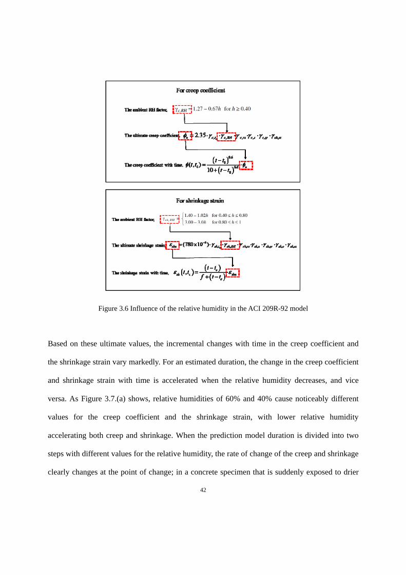
coefficient and ultimate shrinkage strain, as shown in Figure 3.6.

42

Figure 3.6 Influence of the relative humidity in the ACI 209R-92 model

Based on these ultimate values, the incremental changes with time in the creep coefficient and

the shrinkage strain vary markedly. For an estimated duration, the change in the creep coefficient

and shrinkage strain with time is accelerated when the relative humidity decreases, and vice

versa. As Figure 3.7.(a) shows, relative humidities of 60% and 40% cause noticeably different

values for the creep coefficient and the shrinkage strain, with lower relative humidity

accelerating both creep and shrinkage. When the prediction model duration is divided into two

steps with different values for the relative humidity, the rate of change of the creep and shrinkage

clearly changes at the point of change; in a concrete specimen that is suddenly exposed to drier

43

conditions, the change in creep coefficient and the shrinkage strain accelerate markedly as

illustrated in Figure 3.7.(b).

Figure 3.7 The schematic concept of changes in creep and shrinkage rate depending on the RH

The key concept here is that as the relative humidity changes, the ultimate creep coefficient and

shrinkage strain must be updated accordingly in order to incorporate this concept into the

calculation. Ultimately, by taking into account the way the ultimate creep coefficient and

shrinkage strain change with changing relative humidity, results that are closer to the real

behavior should be obtained.

1) Application 1

As an application of this approach, creep and shrinkage prediction has been carried out based on

the ACI 209R-92 model. Except for the relative humidity condition, other factors affecting the

result were assumed to be identical. The four cases, all of which had different relative humidity

conditions, were compared over a period of 100 days. Cases 1 and 2 had constant relative

humidity, and Cases 3 and 4 had relative humidities that varied daily randomly within the ranges

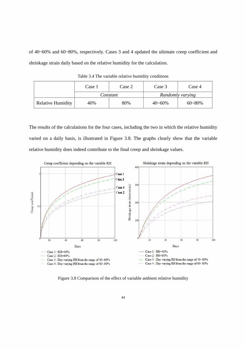
44

of 40~60% and 60~80%, respectively. Cases 3 and 4 updated the ultimate creep coefficient and

shrinkage strain daily based on the relative humidity for the calculation.

Table 3.4 The variable relative humidity conditions

Case 1 Case 2 Case 3 Case 4

Constant Randomly varying

Relative Humidity 40% 80% 40~60% 60~80%

The results of the calculations for the four cases, including the two in which the relative humidity

varied on a daily basis, is illustrated in Figure 3.8. The graphs clearly show that the variable

relative humidity does indeed contribute to the final creep and shrinkage values.

Figure 3.8 Comparison of the effect of variable ambient relative humidity

45

3.3.2 Comparison with experimental data

An experimental investigation of the effect of variable ambient humidity on the creep and

shrinkage of concrete was undertaken by Müller and Pristl (1993), who repeatedly cycled the

humidity condition between 90% and 40% over a period of 100 days, spending a week at each

humidity condition in turn (Figure 3.9), and monitored the resulting creep and shrinkage of a

concrete specimen (Table 3.5). The comparison with the experimental data collected by Müller

and Pristl is presented here to test the accuracy of the proposed new calculation method that

takes into account the effect of changes in the relative humidity. The results for the comparison

of shrinkage strain are shown in Figure 3.10 and Figure 3.11.

Table 3.5 Specimen properties Müller and Pristl (1993)

Concrete specimen properties Diameter = 50mm

Height =100mm

Material properties f’c=40.9 MPa (28-day concrete strength)

Curing condition 7-days moist cured

Relative humidity : Variable

Figure 3.9 Cyclic relative humidity (RH=90 40%)

(From Müller and Pristl, 1993 and used under fair use, 2014)

46

Figure 3.10 Development of shrinkage strain in concrete specimens with diameter of 50mm at variable (RH=90 40%) and constant (RH =65%) ambient humidity (From Müller and Pristl, 1993 and used under fair use, 2014)

Figure 3.11 Comparison of the shrinkage strain results predicted by the proposed method with Müller and Pristl’s (1993) experimental data

The outcome of the comparison of the experimental results with those predicted by the proposed

calculation method can be summarized as follows:

Cyclic relative humidity was applied to investigate the change in shrinkage strain. The

experimental results demonstrate that the concrete specimens are highly affected by large

changes in relative humidity and the resulting pattern of increase and decrease in the

shrinkage strain closely follows the rise and fall of the relative humidity.

Theoretically, concrete swelling due to hydration could occur over an extended time

47

period and this is possible under real-world environmental conditions. However, even

though this is technically feasible under extremely humid or drastically changing

humidity conditions, in practice such exceptional cases are rarely experienced. For this

reason, the swelling effect of concrete is usually ignored in structural analyses. ACI 209

excludes the swelling effect in predicting creep and shrinkage and only relative

humidities close to 99% are considered to be conditions that could cause swelling in CEB

MC90. For the purposes of this research, therefore, it has been determined that swelling

can be ignored for design purposes.

Performing the calculation with the proposed method and varying the humidity every 7

days to replicate the experimental conditions reported by Müller and Pristl (1993), the

ultimate shrinkage strain was updated accordingly. The results of the calculation revealed

that the proposed method follows the real amount of shrinkage fairly well and the rate of

change of the shrinkage strain consistently tracked the variation in the relative humidity.

3.3.3 Summary

Prediction of the time-dependent behaviors of concrete structures subject to creep and shrinkage

is the most uncertain and most difficult aspect of the design process. In particular, creep and

shrinkage are known to be influenced by a number of environmental factors and concrete

properties. Although variations in the ambient relative humidity are not a primary factor

governing the time-dependent behavior of concrete, they do affect the prediction results to some

extent. Given that most existing creep and shrinkage models fail to take variable environmental

conditions into account, it is worthwhile for structural designers to pay renewed attention to the

48

effects of variable ambient conditions and to identify ways to update the existing creep and

shrinkage models accordingly.

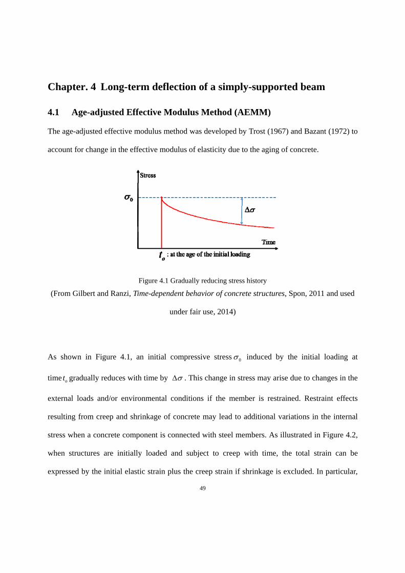
49

Chapter. 4 Long-term deflection of a simply-supported beam

4.1 Age-adjusted Effective Modulus Method (AEMM)

The age-adjusted effective modulus method was developed by Trost (1967) and Bazant (1972) to

account for change in the effective modulus of elasticity due to the aging of concrete.

Figure 4.1 Gradually reducing stress history

(From Gilbert and Ranzi, Time-dependent behavior of concrete structures, Spon, 2011 and used

under fair use, 2014)

As shown in Figure 4.1, an initial compressive stress 0 induced by the initial loading at

time ot gradually reduces with time by . This change in stress may arise due to changes in the

external loads and/or environmental conditions if the member is restrained. Restraint effects

resulting from creep and shrinkage of concrete may lead to additional variations in the internal

stress when a concrete component is connected with steel members. As illustrated in Figure 4.2,

when structures are initially loaded and subject to creep with time, the total strain can be

expressed by the initial elastic strain plus the creep strain if shrinkage is excluded. In particular,

50

the modulus of elasticity changes with the development of the creep strain, and the modulus of

elasticity must therefore be re-established with time so as to account for the increased strain. This

redefined modulus of elasticity is called the effective modulus of elasticity and is expressed by:

1c

e

EE

with : the creep coefficient (4-1)

Figure 4.2 The creep strain and the effective modulus of elasticity

However, the effective modulus of elasticity suffers from the limitation that it cannot reflect the

strain variations that result from the gradually changing stress, so the creep strain produced by a

gradually applied stress will be significantly smaller than that stemming from a stress which is

applied abruptly or maintained constantly over time. This is due to the ageing of the concrete.

Therefore, in order to predict a reasonable value for the creep strain with time for the case of a

gradually applied stress, the age-adjusted effective modulus was developed. This age-adjusted

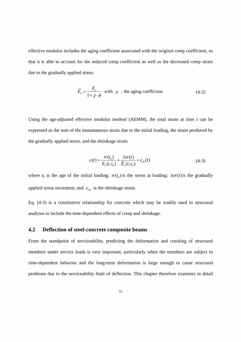
51

effective modulus includes the aging coefficient associated with the original creep coefficient, so

that it is able to account for the reduced creep coefficient as well as the decreased creep strain

due to the gradually applied stress.

1c

e

EE

with : the aging coefficient (4-2)

Using the age-adjusted effective modulus method (AEMM), the total strain at time t can be

expressed as the sum of the instantaneous strain due to the initial loading, the strain produced by

the gradually applied stress, and the shrinkage strain.

0

0 0

( ) ( )( ) ( )

( , ) ( , ) she e

t tt t

E t t E t t

(4-3)

where t0 is the age of the initial loading; 0( )t is the stress at loading; ( )t is the gradually

applied stress increment; and sh is the shrinkage strain.

Eq. (4-3) is a constitutive relationship for concrete which may be readily used in structural

analyses to include the time-dependent effects of creep and shrinkage.

4.2 Deflection of steel-concrete composite beams

From the standpoint of serviceability, predicting the deformation and cracking of structural

members under service loads is very important, particularly when the members are subject to

time-dependent behavior and the long-term deformation is large enough to cause structural

problems due to the serviceability limit of deflection. This chapter therefore examines in detail

52

the analytical procedures for predicting the time-dependent deflection of steel-concrete

composite beams.

4.2.1 Full interaction composite beams

In steel-concrete composite beams, when a combined axial force and bending moment are

applied to the composite beam leading to time-dependent deformations that develop due to the

effects of creep and shrinkage on concrete, both the instantaneous and time-dependent strains

and curvatures can be calculated using the AEMM. The variations in strain and curvature of the

cross-section are known at regular intervals along the beam, so it is relatively simple to

determine the deflection of that member. To apply this process to the analysis, a composite beam

model is utilized, based on the following assumptions.

A simply-supported steel-concrete composite beam is subject to sustained, uniformly

distributed loadings for entire time interval.

The short-term deformations are instantaneously developed at the age of the initial

loading and the effects of creep and shrinkage generate long-term deformations. The two

deformations are calculated separately.

For a composite beam in which the steel and concrete components are connected with a

sufficient number of shear connectors, complete shear interaction is assumed, which

means that there is no relative slip on the interface and the composite beam behaves in a

fully composite fashion.

Cross-sectional properties of the composite cross-section are calculated based on the

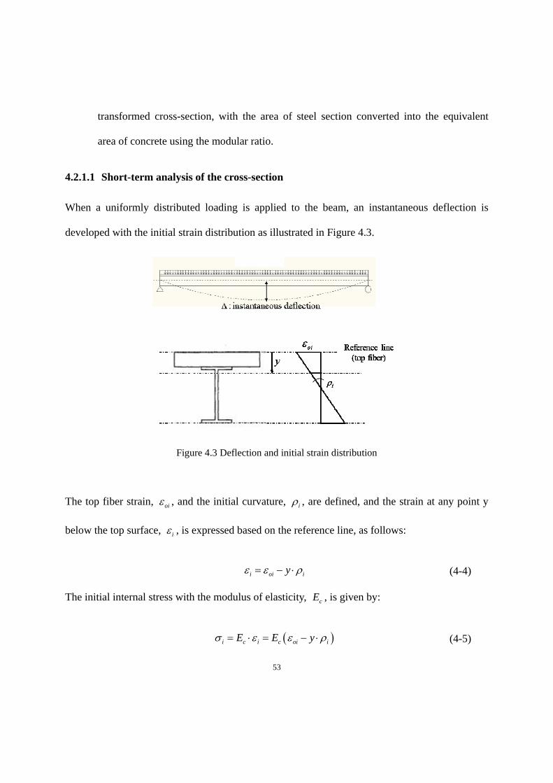
53

transformed cross-section, with the area of steel section converted into the equivalent

area of concrete using the modular ratio.

4.2.1.1 Short-term analysis of the cross-section

When a uniformly distributed loading is applied to the beam, an instantaneous deflection is

developed with the initial strain distribution as illustrated in Figure 4.3.

Figure 4.3 Deflection and initial strain distribution

The top fiber strain, oi , and the initial curvature, i , are defined, and the strain at any point y

below the top surface, i , is expressed based on the reference line, as follows:

i oi iy (4-4)

The initial internal stress with the modulus of elasticity, cE , is given by:

i c i c oi iE E y (4-5)

54

The initial axial force, N, and the bending moment about the top surface, M, are expressed by:

iN dA (4-6)

c oi c iN E A E B (4-7)

iM ydA (4-8)

c oi c iM E B E I (4-9)

where A, B, and I are the cross-sectional properties of the transformed section and correspond to

the area, and the first and second moments of area about the top reference surface, respectively.

For this cross-section, where only a uniformly distributed loading is applied, no resultant axial

force is generated and the internal moment about the top surface is identical to the external

bending moment. Rearranging Eq. (4-7) and Eq. (4-9), the short-term strain distribution and

curvature are obtained and can be expressed in terms of the applied force, N, and the bending

moment, M.

The initial top fiber strain is:

2oi

c

B M I N

E A I B

(4-10)

The initial curvature is:

2i

c

A M B N

E A I B

(4-11)

If the simply-supported member is subject to both axial and transverse loads and the curvatures

55

of the cross-section are provided, the deflection at any point along the member can be obtained

by integrating the curvatures throughout the length of the member (Figure 4.4)

Figure 4.4 Deflection of a simply-supported beam

In particular, if the curvature at the mid-span and at each support is known, the deflection at mid-

span mid initial is given by:

2

1096mid initial A mid C

L

(4-12)

A parabolic variation of curvature along the beam is assumed in this equation.

This method may be generally applied to all types of simply-supported beams under uniformly

distributed loading as long as elastic behavior can be assumed for the short-term analysis. For the

case of deflection in a steel-concrete composite beam, an alternative method introduced in AISC

can be recommended. For short term deflections, AISC proposes a lower bound elastic moment

56

of inertia, LBI , for plastic composite sections, and if the loading condition is determined, one may

calculate the mid-span deflection, as given in Eq. (4-13)

45

384 s LB

wL

E I (4-13)

4.2.1.2 Time-dependent analysis using the AEMM

The advantage of using the AEMM is that it can cope with the variations in stresses and strains

with time due to creep and shrinkage of concrete in steel-concrete composite cross-sections.

From the first loading onwards, creep and shrinkage strains develop in the concrete and the

gradual change of strain in the concrete with time results in changes in the stress within the steel

cross-section. In general, there is a gradual increase in the compressive stress in the steel part as

the concrete shrinks due to the effects of creep and shrinkage. At this point, the internal stresses

are redistributed and the gradual change of force in the steel is countered by an equal and

opposite restraining force on the concrete in order to maintain equilibrium. These resultant

restraining forces induced by creep and shrinkage on the concrete are defined as the change in

the axial force, N , and the change in moment about the reference axis, M . By applying three

structural basic conditions, namely equilibrium, compatibility, and the constitutive laws, either

the short- or the long-term deformations can be ultimately obtained. This approach to analyzing

the time-dependent behavior of steel-concrete composite structures has been used in many

previous studies, and in the current research the method presented by Gilbert (1989) is applied.

Figure 4.5 indicates the time-varying strain distributions along the cross-section and the

57

increasing deformations with time, respectively.

Figure 4.5 Instantaneous and time-dependent strain distribution for a steel-concrete cross-section

For the restraining actions, the constitutive relationship at any time, t, must be satisfied for both

the restraining forces and the time-dependent deformations:

( )( ) ( )c oi c i sh cN Ee t A B t A (4-14)

( )( ) ( )c oi c i sh cM Ee t B I t B (4-15)

where Ac, Bc, and Ic are the cross-sectional properties of concrete only; and ( )t and ( )sh t are

the creep coefficient and the shrinkage strain at time, t, respectively.

The reason that the cross-sectional properties of concrete are used in Eq. (4-10) and (4-11), is

that the effects of creep and shrinkage develop only in the concrete component; the steel is

unaffected.

58

As stated above, after the initial loading is applied and the instantaneous strain and curvature

have been determined, the axial force N and the moment M are responsible for the additional

time-varying deformations on the cross-section with increasing time. During this time-dependent

analysis, the AEMM is able to account for variations in creep and shrinkage effectively by

requiring the modular ratio of /s cE E to be revised for the transformed cross-section analysis.

Since the modular ratio varies according to the age-adjusted effective modulus, the transformed

cross-sectional properties must also be re-defined and A, B, and I are therefore modified as

, , and e e eA B I , respectively.

Using the axial force N , the moment M and the re-defined cross-sectional properties

associated with the age-adjusted effective modulus, eE , the following equations in terms of the

time-dependent strain and curvature can be established:

The additional top fiber strain is:

2e e

o

e e e e

B M I N

E A I B

(4-16)

The additional curvature is:

2e e

e e e e

A M B N

E A I B

(4-17)

In addition to initial deformations, the increased deflection of the beam due to creep and

shrinkage is calculated as:

59

2

1096mid increased A mid C

L (4-18)

Where increased is the increased mid-span deflection; and , , and A mid C are the additional

curvatures at each point along the member.

Finally, the total time-dependent deformations can be obtained by adding the time-dependent

strain, curvature and the deflection to the given initial values.

The total top fiber strain is:

o total oi o (4-19)

The total curvature is:

total i (4-20)

The total deflection is:

total mid initial mid increased (4-21)

4.2.2 Partial composite beams

To evaluate the time-dependent behavior of steel-concrete composite beams, fully composite

action for which no slip occurs on the interface between steel and concrete has been assumed so

far. However, this complete shear interaction for a composite beam can be achieved only when

there are sufficient shear connectors or studs to resist the occurrence of slip, and in practice it

may not always be necessary to enforce full shear interaction. In real construction applications,

the number of shear connectors required to achieve full shear interaction may be so large that it is

60

not practical to accommodate them in a composite beam due to the associated problems of cost

and workability. Therefore, the current design provisions generally allow some slip effects in

composite structures as long as these remain within safety limits for serviceability and many

engineers focus instead on controlling the amount of slip and the resultant behavior effectively.

When considering the serviceability of composite beams, the partial composite action is

connected with a deflection problem as a composite beam with partial shear interaction has a

higher deflection than a beam with complete shear interaction. The remainder of this chapter

deals first with the approximate method for calculating the deflection due to slip effects for the

short-term deflection due to immediate loading and then moves on to look at the long-term

deflection resulting from creep and shrinkage.

Figure 4.6 (a) Slip of a composite beam, (b) Strain distribution with slip

(From Wang, Deflection of steel-concrete composite beams with partial shear interaction,

Journal of Structural Engineering, 1998 and used under fair use, 2014)

61

4.2.2.1 Short-term analysis with slip

Figure 4.7 Shear force developed on the interface and strain distribution with the slip

When service loads are applied instantaneously, a shear force between steel and concrete

components is developed horizontally along the beam unless the slip is prevented totally by the

addition of sufficient stiff shear connectors. If this is not the case, the total strain distribution is

determined by adding the slip strain to the initial strain at the steel-concrete interface. This

process is illustrated in Figure 4.7.

The overall procedure for calculating the strain and curvature of the composite cross-section is

very similar to that for the analysis of a fully composite beam with complete shear interaction.

The transformed section analysis for the top fiber surface is identically adopted and a uniformly

distributed loading is assumed to act on a simply-supported beam. The only difference is that slip

must be taken into account when applying the constitutive laws and compatibility, so the

following set of equations for a short-term analysis with slip can be established.

62

The short-term strain i at any depth y from the top fiber surface is

In the concrete slab:

0i i iy (4-22)

In the steel section:

i oi slip iy (4-23)

The force cN in the concrete section and the force sN in the transformed steel section are

0

0

cy D

c c i

y

c c i c c i

N E d A

E A E B

(4-24)

( )

c

c

y D h

s c i

y D

c s oi slip c s i

N E d A

E A E B

(4-25)

where Dc and h are the depths of the concrete slab and the steel beam, respectively, and Ec is the

modulus of elasticity of concrete.

Only pure bending force is acting on the beam and there is no axial force, so the equilibrium

conditions are satisfied as follows:

0c sN N (4-26)

Rearranging Eq. (4-24) ~ Eq. (4-26), the strain at the top of the composite sample is given by:

63

0

( )

( )c s i s slip

ic s

B B A

A A

(4-27)

For a slice of the member along the interface, the horizontal shear force F equals the force cN in

the concrete slab. Substituting Eq. (4-27) into Eq. (4-24) gives:

c c s

c c c i c slip

A B A AN E B E F

A A

(4-28)

where A = Ac + As and B = Bc + Bs, both of which are associated with the transformed cross-

section.

The bending moment about the top reference line is

0

2

c c

c

y D y D h

c i c i

y y D

sc i c s slip

M E y d A E y d A

A BBE I E B

A A

(4-29)

Applying the above equations to obtain the slip strain, an approximate approach that assumes

that the shear force Q at each connector has an average value along the member and that there is

a linear relationship between the amount of slip and the longitudinal force at the connectors is

utilized. The whole process is as follows.

1) If the initial slip strain due to the applied loads is assumed to be very small, the initial

64

curvature can be determined because the moment M is known from statics using Eq.

(4-29).

2) By substituting the initially assumed slip strain and the obtained curvature into Eq. (4-28),

the total longitudinal force F acting on the interface is determined.

3) Assuming that this total longitudinal force F is resisted by the sum of the shear

connectors, the average force Qaverage acting on each connector is expressed by:

No. of the shear studs

FAverage Q

4) Several approaches have been suggested to define the relationship between the

longitudinal force Q and the slip. In Table 4.1, the methods proposed by Ollgaard et al.

(1971) and Bradford and Gilbert (1992) are applied to obtain the average slip slip at each

connector.

Table 4.1 The relationship between the longitudinal force Q and the slip

Q Kc

(Bradford & Gilbert 1992)

18 2/5(1 )Q Qu e

(Ollgaard, Slutter, and Fisher 1971)

Kc=84 kN/mm for a shear stud with a diameter of 0.5 in.

Kc is considered to be the slope of a secant line for a fairly small slip

Qu = the ultimate strength of the shear connectors; Kc = the modulus of the connector; and = the amount of slip at the interface.

5) Given the amount of the slip, a new value for the slip strain is calculated:

65

slip

Slip

Corresponding Length

(4-30)

6) Steps (1) ~ (5) are repeated iteratively until the slip strains converge at each section.

7) Once the slip strains have been determined by iteration, the additional curvatures due to

the slip can be calculated:

( )slip

slipcD h

(4-31)

Figure 4.8 (a) Final strain with the slip, (b) Strain without the slip, (c) Slip strain only

8) The final curvature, including the effects of the slip, is the sum of the initial curvature

without the slip and the additional curvature due to the slip.

, non- , i i slip i slip (4-32)

66

9) Using the obtained curvature for each section, the mid-span final deflection that includes

both the initial deflection and the additional deflection resulting from the slip is finally

calculated using Eq. (4-12) and Eq. (4-18).

4.2.2.2 Time-dependent analysis with slip

When the restraining forces and N M due to creep and shrinkage are released from the cross-

section, the strain distribution changes and additional deformations occur. These released forces

also add to the slip strain if the beam acts in a partially composite fashion. By adopting an

iteration scheme for the time-dependent slip strain, as was done when determining the short-term

slip strain, the time-dependent slip strain and curvature are also obtained. Ultimately, the final

curvature with time-dependent slip is determined by combining the initial curvature with the slip,

the additional time-dependent curvature without the slip, and the time-dependent curvature with

the slip. That is:

0 time dependent i slip (4-33)

where i is the short-term curvature including the slip; 0 is the long-term curvature without

the slip; and slip is the long-term curvature with the slip.

Given the time-dependent curvature, the final deflection with time can be determined for the case

of a partially composite beam subject to creep and shrinkage. In order to show the effects of the

slip, a simple application example of the time-dependent analysis of partially interactive beams is

introduced here. Figure 4.9 indicates the divergent results in the mid-span deflection of simply-

supported composite beams varying according to the degree of the partial interaction, and the

67

variables for calculation are assumed as shown in Table 4.2.

Table 4.2 Input variables for the application example

Cross-sectional properties

Effective width=96in

Depth of concrete deck=4.5in

Depth of steel beam=17.75in

Area of steel beam =10.3in2

Moment of inertia of steel beam =510 in4

Material properties

f’c=4000 psi (28-day concrete strength)

Ec=3644 ksi

Es=29,000 ksi

Curing condition 7-days moist cured

Relative humidity = 60%

Loading &

Boundary condition

Uniformly distributed load , W=0.638 k/ft

Simply supported beam

Span length L=380 in (96ft)

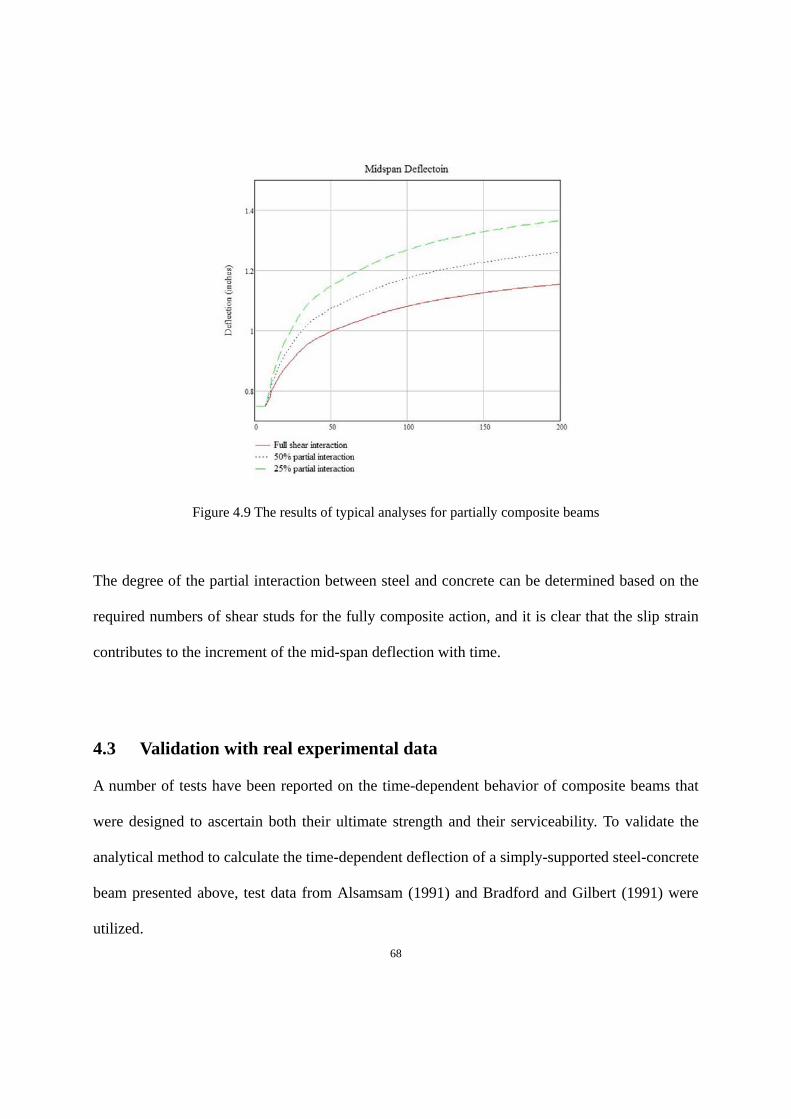
68

Figure 4.9 The results of typical analyses for partially composite beams

The degree of the partial interaction between steel and concrete can be determined based on the

required numbers of shear studs for the fully composite action, and it is clear that the slip strain

contributes to the increment of the mid-span deflection with time.

4.3 Validation with real experimental data

A number of tests have been reported on the time-dependent behavior of composite beams that

were designed to ascertain both their ultimate strength and their serviceability. To validate the

analytical method to calculate the time-dependent deflection of a simply-supported steel-concrete

beam presented above, test data from Alsamsam (1991) and Bradford and Gilbert (1991) were

utilized.

69

4.3.1 Comparison with the test data from Alsamsam (1991)

Alsamsam examined the use of an analytical tool for composite floor systems for instantaneous

and time-dependent deflections, concrete slab differential shrinkage, and creep effects due to

sustained loads. The analysis was then verified by a full-scale experimental testing program

involving four 32 ft. simply supported composite beam specimens with a full interaction over a

period of 200 days. To compare the mid-span deflection of the beam with the full shear

interaction, the process described in Chapter 4.2.1 was used here and the instantaneous deflection

due to the dead loads at 0 days calculated, taking into consideration the unshored construction.

The values for creep coefficient and shrinkage strain needed for the time-dependent analysis

were taken from ACI 209R-92, and the modification introduced in Chapter. 3.3 applied to reflect

the actual ambient relative humidity recorded in the laboratory.

4.3.1.1 Description of the test

Each specimen consisted of a W18x35 beam with a 4.5-in-thick and 96-in-wide slab on a 3-in

steel deck. The composite beams were 32 ft long and were designed to be fully composite, with

A36 steel and a concrete compressive strength of 4 ksi, utilizing normal-weight concrete. Two

beams, which were unshored during casting, were chosen to monitor long-term creep and

shrinkage, and an additional sustained load equal to about 25% of the design live load was

applied to one of the two beams at 10 days after casting. The details of the experiment are shown

below in Table 4.3 ~ Table 4.6 and Figure 4.10 and Figure 4.11.

70

Table 4.3 Construction conditions

Specimen Number Support Condition Shoring Age Tested (days)

Beams #1 and #2 Rollers Unshored 200 days

Table 4.4 Concrete mix variables and curing conditions

Specimen Number Beam #1 and #2

Curing type Moist

Cement type Type I

Fines (%) 35%

Air content (%) 6%

Slump (in.) 4 in.

Relative humidityBased on the real

record during 200 days

71

Figure 4.10 Ambient relative humidity condition

(Alsamsam, 1991)

Figure 4.11 Cross-section and elevation of the beam

72

Table 4.5 Cross-sectional properties

Beam #1 and #2

Steel depth, h 17.75 in.

Steel area, As 10.3 in2

Moment of inertia of steel, Is 510 in4

Modulus of elasticity of steel, Es 29,000 ksi

Strength of steel, Fy 36 ksi

Concrete slab depth, Dc 4.5 in.

Width of concrete 96 in.

Concrete weight, Wc 145 pcf

Modulus of elasticity of concrete, Ec 3,644 ksi

Strength of concrete, 'cf 4 ksi

Depth of the deck rib, Dr 3 in.

Aging coefficient, 0.85

* Ribs are perpendicular to the beam, therefore the concrete in the ribs of the deck are ignored

Table 4.6 Loading conditions

Beam #1 Beam #2

Dead load 0.64 kips/ft 0.64 kips/ft

Live load 1.5 kips/ft -

Span length 380 in. 380 in.

73

4.3.1.2 Results

1) Instantaneous mid-span deflection

For the unshored construction, the dead load deflection at casting due to the weight of the wet

concrete slab is carried by the steel beam only. Thus:

450.976 .

384D

Ds s

W Lin

E I

(4-34)

Alsamsam assumed 75% of the estimated dead load deflection as the reduction to account for

possible stiffening effects from the end connections, so the initial deflection at 0 days is (0.976 x

75%) = 0.732 in.

The instantaneous deflection at 10 days due to the additional sustained loading can be obtained

by Eq. (4-10) ~ (4-12), and the value is predicted to be 0.126 in. accordingly. This immediate

deflection is close to the experimental value of 0.1 in.

Table 4.7 Comparison of instantaneous mid-span deflection

Time Experimentally measured

deflection Calculated deflection

0 days (at casting) 0.75 in. 0.732 in.

10 days (under additional loading)

0.1 in. 0.126 in.

74

2) Creep and shrinkage with time (ACI 209R-92)

Based on the actual recorded relative humidity, the creep coefficient and shrinkage strain for the

long-term analysis were determined (Figure 4.12).

Figure 4.12 Creep coefficient and shrinkage strain, using ACI209R-92

75

3) Time-dependent mid-span deflection

Figure 4.13 Comparison of time-dependent deflection for the test data and the proposed method

Table 4.8 Comparison of the mid-span deflection 200 days after casting

Experimentally

measured deflectionCalculated deflection

Beam 1 (only dead load) 1.192 in. 1.152 in.

Beam 2 (additional load) 1.302 in. 1.277 in.

In summary, the proposed method for predicting the time-dependent deflection of the full

76

composite beams introduced in Chapter 4.2.1 has been verified by comparing the results with the

experimental test data reported by Alsamsam (1991). Although the long-term deflection obtained

from the proposed method is somewhat lower than those measured by Alsamsam, the prediction

using the proposed method matches the experimental data fairly well for both the short- and the

long-term mid-span deflection.

4.3.2 Comparison with the test data of Bradford and Gilbert (1991)

Bradford and Gilbert conducted a series of tests on four simply-supported steel-concrete

composite beams. The four simply supported beams were monitored for about 200 days to

observe the effects of creep and shrinkage, together with the effects of the shear studs employed

to examine the behaviors of the partially bonded steel-concrete composite beams. For the

analysis of the deflection of the partial composite beams, the process in section 4.2.2 was used.

4.3.2.1 Description of the test

Two beams (B1 and B3) were loaded using a superimposed sustained uniformly distributed load

of 7.52 kN/m, while the remaining two beams (B2 and B4) were subject to self-weight only. Two

beams (B1 and B2) were designed to have nearly full interaction, with pairs of studs at 200 mm

intervals along the beam, and the remaining two beams (B3 and B4) were designed with pairs of

studs at 600 mm so that substantial slip is likely to take place. All beams were moist-cured for 10

days after casting and were fully propped during this period. Among the four specimens, only B1

and B3 will be used here; both were loaded with 7.52 kN/m and B3 is considered to be a partially

composite beam. The experimental conditions are shown below in Figure 4.14 and Table 4.9 ~

Table 4.11.

77

Figure 4.14 Test set up (a) elevation, (b) cross-section, (c) stud

(From Bradford and Gilbert, Time-dependent behavior of simply-supported

steel-concrete composite beams, 1991 and used under fair use, 2014)

Table 4.9 Information on creep and shrinkage

Creep coefficient 2.55

Ultimate shrinkage 6410 10shu

Aging coefficient 0.85

Table 4.10 Cross-sectional properties

Steel depth, h 200 mm

Steel area, As 3230 mm2

Moment of inertia of steel, Is 2,360 x 104 mm4

Modulus of elasticity of steel, Es 200,000 MPa

Concrete slab depth, Dc 70 mm

Width of concrete 1,000 mm

Modulus of elasticity of concrete, Ec 25,000 MPa

Strength of concrete, 'cf 27.6 MPa

78

Table 4.11 Loading conditions and shear studs

Beam B1 Beam B3

Dead load 2.0 kN/m 2.0 kN/m

Live load 7.52 kN/m 7.52 kN/m

Span length 5,900 mm 5,900 mm

Shear stud interval 200 mm

(nearly full composite)

600 mm

(partial composite)

4.3.2.2 Results

Both the full (200mm interval) and partial (600 mm interval) shear interactions are examined, so

here the calculation is also separately applied to compare the differences between the two.

1) Short-term deflection

Beam B1 was designed to be fully composite and the short-term deflection can be obtained by

means of Eq. (4-10) ~ (4-12), predicting a mid-span deflection of 10.69 mm at the age of loading.

Unlike B1, only partially composite action is assumed for B3, and the B3 shear stud interval of

600 mm results in only approximately 30% of the full interaction between steel and concrete.

Applying the process from section 4.2.2.1, the short-term deflection of the mid-span is predicted

to be 11.22 mm, much larger than the deflection without the slip.

79

Table 4.12 Results of the short-term mid-span deflection

Experimentally measured deflection Calculated deflections

Beam B1 Beam B3 Beam B1 Beam B3

Studs at 200 mm

(fully composite)

Studs at 600 mm

(partially composite)

Fully composite analysis

Partially composite analysis

9.3 mm 11 mm 10.69 mm 11.22 mm

2) Time-dependent mid-span deflection

The partially composite analysis taking into account the time-varying creep and shrinkage as

well as the slip effects, discussed above in Chapter 4.2.2.2, yields the results shown in Figure

4.15.

Figure 4.15 Comparison of time-dependent deflection for the test data and the proposed method

80

Table 4.13 Comparison of the mid-span deflection after 250 days

Experimentally measured deflection Calculated deflection

Beam B1 Beam B3 Beam B1 Beam B3

Studs at 200 mm

(fully composite)

Studs at 600 mm

(partially composite)

Fully composite analysis

Partially composite analysis

22.4 mm 23.4 mm 22 mm 22.9 mm

The results of the analytical approach for the short-term and time-dependent response of a simply

supported composite beam that was developed for full and partial shear interactions were

compared with the results of experimental tests on composite beams reported by Bradford and

Gilbert (1991). The agreement between the test and the proposed method is shown to be good.

81

Chapter. 5 Parametric study

There are a number of factors that affect the structural response of steel-concrete composite

beams, and current design provisions neither incorporate well-established equations for

predicting the effects of creep and shrinkage nor specify serviceability criteria for long-term

deformations. AISC included no suggestions for calculating the long-term deformations

associated with creep and shrinkage before 2001, and it was not until 2005 that a brief

recommendation was included in the commentary. Similarly, ACI only proposes prescriptive

methods calibrated to older data, which may not be sufficiently reliable to calculate the long-term

deformations of composite members. Based on the current situation, where neither AISC nor

ACI provides a reasonable method incorporating the various effects of the related-variables for

the time-dependent analysis of composite structures, a concerted effort to define a correlation

between the effects of various variables and the resultant structural response in more detail is

clearly overdue. In this context, the parametric studies presented in this section will be used to

estimate the effect of the many variables used in a practical design to account for the long-term

deformations of composite beams due to creep and shrinkage.

5.1 Parameter setting

Of the wide variety of variables involved, the most frequently-used in construction utilizing

steel-concrete composite beams will be examined, namely the properties of concrete, structural

configuration of the composite beams, and the type of loading. These are discussed in turn below.

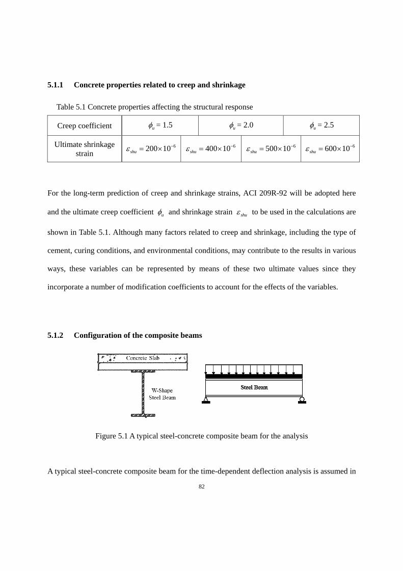
82

5.1.1 Concrete properties related to creep and shrinkage

Table 5.1 Concrete properties affecting the structural response

Creep coefficient u = 1.5 u = 2.0 u = 2.5

Ultimate shrinkage strain

6200 10shu 6400 10shu 6500 10shu 6600 10shu

For the long-term prediction of creep and shrinkage strains, ACI 209R-92 will be adopted here

and the ultimate creep coefficient u and shrinkage strain shu to be used in the calculations are

shown in Table 5.1. Although many factors related to creep and shrinkage, including the type of

cement, curing conditions, and environmental conditions, may contribute to the results in various

ways, these variables can be represented by means of these two ultimate values since they

incorporate a number of modification coefficients to account for the effects of the variables.

5.1.2 Configuration of the composite beams

Figure 5.1 A typical steel-concrete composite beam for the analysis

A typical steel-concrete composite beam for the time-dependent deflection analysis is assumed in

83

this analysis, as illustrated in Figure 5.1. The composite beam is connected by shear connectors

and a uniformly distributed load is applied to the beam with simply supported boundary

conditions. The characteristics of the beam are shown in Table 5.2.

Table 5.2 Configuration of the composite beam

Size of the steel beam

W18x35 W21x55 W27x94

Span length 24 ft 28 ft 32 ft 36 ft 40 ft

Degree of composite action

100%

Fully composite

50%

Partial composite

25%

Partial composite

5.1.3 Other factors

1) Floor system

Effective width (be) of the composite beam = Span length/4

Table 5.3 Effective width according to the span length

Span length 24 ft 28 ft 32 ft 36 ft 40 ft

Effective width 72 in. 84 in. 96 in. 108 in. 120 in.

The floor on which the uniformly distributed loads are applied is a square-bay frame.

2) Loading conditions

A uniformly distributed loading is considered for the floor of a square-bay frame, and the loads

84

acting along the beam are determined by the length of each bay.

The dead load from self-weight of the beam is ignored as it can be taken out by

cambering during manufacturing.

The superimposed dead load is determined by the sum of the mechanical and electrical

piping (10 psf), ceiling (10 psf), and floor finishes (5 psf).

The design live load for a common floor system for office buildings is assumed to be 50

psf.

The sustained load for the time-dependent behaviors is considered to be the superimposed

dead load plus 30% of the design live load.

For service loads, no load factors are applied to service checks, which means all loads are

1.0 x (Dead load) + 1.0 x (Live load).

Table 5.4 Loading configuration

Dead Load Self-weight N/A

Superimposed dead load 25 psf

Live Load Office building 50 psf

Sustained Load

Superimposed dead load plus 30% of design live load 40 psf

3) Other assumptions

The aging coefficient for the age-adjusted effective modulus is assumed to be 0.85.

85

The 28-day compressive strength of concrete is 4 ksi.

The modulus of elasticity of steel is 29,000 ksi.

The shear modulus for 0.5 in.-shear stud is close to 450 kips/in, based on reported test

results (Bradford and Gilbert 1992).

Time duration to be considered for the long-term analysis is 250 days.

5.2 Analysis and results

All the calculations were performed using a MathCAD simulation, and the following three issues

were analyzed.

Immediate deflection limitation due to the instantaneous live load.

The ratio of the long-term deflection to the short-term deflection due to creep and

shrinkage.

Comparison with AISC simple model to predict the long-term deflection due to creep and

shrinkage.

5.2.1 Short-term deflection due to the immediate design live load

A uniformly distributed load, 50 psf, is considered to be a full design live load and applied to a

series of the composite beams. To calculate the initial mid-span deflection, a lower bound

moment of inertia LBI is used; AISC proposes a lower bound moment of inertia for a realistic

short-term deflection of composite flexural members. The ILB is given in Table 3-20 in the 13th

edition of the Steel Construction Manual from AISC. Thus, the immediate mid-span deflection is

86

given by:

45

( )384

LLLive load short term

s LB

W L

E I

(5-1)

where (50 ) ( )LLW psf Length of Bay

L Length of Span

The obtained mid-span deflection is compared in Table 5.5 through 5.7 with Table 9.5(b)

Maximum Permissible Computed Deflections in ACI 318-11 in order to check the serviceability

limit state. In this case, the allowable deflection due to a live load is L/360. This is the most

common limit assumed to check floor deflections due to live load.

Table 5.5 Full interaction beams; immediate deflection limitation check due to live load

Beam (in.) W18x35 W21x55 W27x94

Span length (ft) 24 28 32 28 32 36 32 36 40

Immediate load (k/ft)

1.2 1.4 1.6 1.4 1.6 1.8 1.6 1.8 2.0

L/360 (in.) 0.80 0.93 1.07 0.93 1.07 1.20 1.07 1.20 1.33

Obtained immediate

deflection (in.) 0.21 0.45 0.85 0.23 0.43 0.80 0.17 0.30 0.52

87

Table 5.6 50% partial interaction beams; immediate deflection limitation check due to live load

Beam (in.) W18x35 W21x55 W27x94

Span length (ft) 24 28 32 28 32 36 32 36 40

Immediate load (k/ft)

1.2 1.4 1.6 1.4 1.6 1.8 1.6 1.8 2.0

L/360 (in.) 0.80 0.93 1.07 0.93 1.07 1.20 1.07 1.20 1.33

Obtained immediate

deflection (in.) 0.26 0.57

1.11

(N.G)0.29 0.56 1.00 0.21 0.38 0.64

Table 5.7 25% partial interaction; immediate deflection limitation check due to live load

Beam (in.) W18x35 W21x55 W27x94

Span length (ft) 24 28 32 28 32 36 32 36 40

Immediate load (k/ft)

1.2 1.4 1.6 1.4 1.6 1.8 1.6 1.8 2.0

L/360 (in.) 0.80 0.93 1.07 0.93 1.07 1.20 1.07 1.20 1.33

Obtained immediate

deflection (in.) 0.34 0.74

1.44

(N.G)0.36 0.70

1.26

(N.G)0.26 0.46 0.79

Table 5.5 shows the deflection on the full interaction composite beams. None of the obtained

deflection values exceeded the L/360 criteria. This indicates that the steel-concrete composite

beams with the most widely-used sizes and spans for building floor systems exhibit a good

performance in their structural serviceability if the beams are designed for full composite action.

In fact the most economical sections are those with partial interaction in the range of 30% to

88

50%.

Table 5.6 and Table 5.7 show the cases for the beams designed to 50% and 25% interaction,

respectively. The composite beams with W18x35 and W21x55 of steel beam exceeded the

deflection criteria under the sustained live loads acting on the 32ft- and 36ft-span beams. This

may imply that considerable attention has to be needed for serviceability limit state, in case that

the composite beams whose span lengths are fairly long and have a relatively light and shallow

steel beam.

Therefore, when considering a typical immediate design live load for a common floor system for

office buildings, it can be said that the most recommendable combinations of the size of steel

beams and the span length are as shown in Table 5.8.

Table 5.8 Reasonable combinations of the size of steel beams and span length

Full shear interaction 50% Partial interaction 25% Partial interaction

W18x35 32 ft 28 ft 28 ft

W21x55 36 ft 32 ft 32 ft

W27x94 40 ft 40 ft 40 ft

* Loading conditions: Design live load = 50 psf

5.2.2 The ratio of the long-term and short-term deflections due to creep and shrinkage

Although the short-term deflection can be easily obtained by Eq. (5-1), it is still not

straightforward to predict the long-term deflection due to creep and shrinkage under the

sustained service loads. Thus, in this section the ratio of the long-term deflection to the short-

89

term deflection will be examined under realistic service load conditions. This result may be

helpful for predicting the long-term deflection approximately based on its short-term values. The

loading conditions for the analysis are set up as shown below in Figure 5.2.

Figure 5.2 (a) Loading for the short-term deflection, (b) Loading for the long-term deflection

The ratio of the long-term deflection to the short-term deflection, long term

short term

, is comprehensively

summarized in Tables 5.9 ~ 5.11.

90

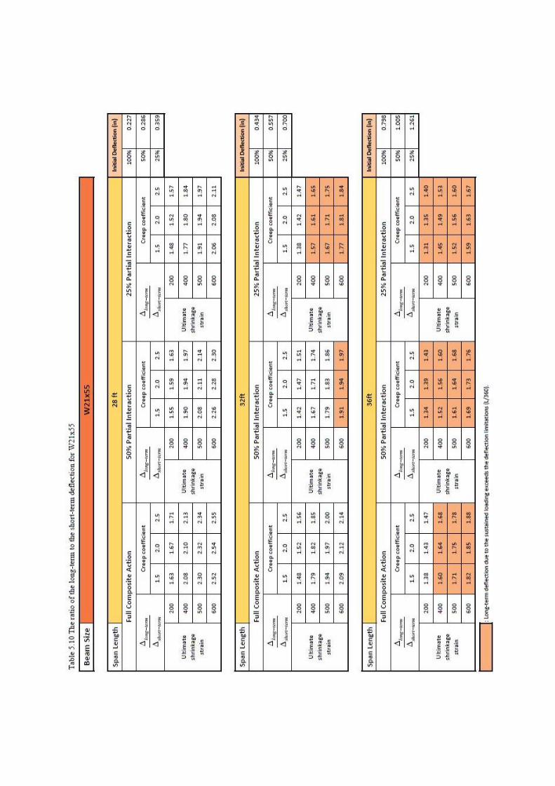
91

92

93

The results of the parametric analyses in Tables 5.9 ~ 5.11 imply that

the ratio of the short-term deflection to the long-term deflection covers a range of

approximately 1.5 ~ 2.5, which means that the long-term mid-span deflection of a steel-

concrete composite beam is about 1.5 ~ 2.5 times its short-term deflection,

as the effects of creep increase, although the long-term deformation also increases, the

increment in the long-term value is relatively small,

the effects of shrinkage may contribute much more to the time-dependent deformation

than the effect of creep for cases where the sustained live load is 30%,

a composite beam with a partial shear interaction exhibits a larger mid-span deflection for

both the short- and long-term deflections than a beam with a full shear interaction.

When it comes to the deflection limitations, it turned out that although the short-term deflections

due to the immediate design live load satisfy the deflection criteria well, its long-term deflections

can exceed the deflection limitations. In addition, it is generally agreed that design for the

composite beams is not governed by strength limit state. Therefore, when considering the

sustained loading for about 250 days, it can be summarized that the reasonably recommendable

combinations of the size of steel beams and the span length are as follows.

94

Table 5.12 Reasonable combinations of the size of steel beams and span length

Full shear interaction 50% Partial interaction 25% Partial interaction

W18x35 28 ft 24 ft 24 ft

W21x55 32 ft 28~32 ft 28 ft

W27x94 40 ft 40 ft 36 ft

* Loading conditions: Sustained loads = 40 psf

5.2.3 Comparison with AISC simple model to predict the long-term deflection

AISC (Commentary I3 in the 13th edition of the Steel Construction Manual from AISC)

proposes a simple method to predict the long-term deflection due to creep and shrinkage, and

according to AISC, if the restrained shrinkage coefficient for the aggregates is not known, the

shrinkage strain for these calculations may be taken as 0.02%. AISC basically uses shrinkage

force coming from shrinkage strain of concrete and assumes a uniform moment along the beam

associated with corresponding eccentricity. The long-term deformation due to shrinkage can be

calculated with the simplified model in AISC, as shown in Figure 5.3.

95

Figure 5.3 Calculation of shrinkage effects

(From AISC Fig. C-I3.2 and used under fair use, 2014)

To compare the AISC simple model with the proposed method in Chapter. 4, the variable

conditions are identically set up each other and analysis for predicting the long-term deflection is

carried out. For AISC calculation, a lower bound moment of inertia is used. The results are

described in Table 5.13 ~ 5.15.

Table 5.13 Long-term deflection from AISC simple model and the proposed method for W18x35

Beam size : W18x35

Span length 24 ft 28 ft 32 ft

Long-term deflection

(Proposed method) 0.21 in. 0.30 in. 0.42 in.

Long-term deflection

(AISC method) 0.14 in. 0.20 in. 0.26 in.

96

Table 5.14 Long-term deflection from AISC simple model and the proposed method for W21x55

Beam size : W21x55

Span length 28 ft 32 ft 36 ft

Long-term deflection

(Proposed method) 0.24 in. 0.33 in. 0.45 in.

Long-term deflection

(AISC method) 0.15 in. 0.21 in. 0.27 in.

Table 5.15 Long-term deflection from AISC simple model and the proposed method for W27x94

Beam size : W27x94

Span length 32 ft 36 ft 40 ft

Long-term deflection

(Proposed method) 0.22 in. 0.30 in. 0.39 in.

Long-term deflection

(AISC method) 0.13 in. 0.18 in. 0.23 in.

In case of the full composite beams, the long-term deflection obtained by the AISC method is

smaller than that from the proposed method. Therefore, the results of the parametric analyses in

Tables 5.13 ~ 5.15 imply that the AISC simple model to predict the long-term deflection tends to

underestimate the effect of shrinkage with time, especially in case of the full composite beams.

97

Chapter. 6 Conclusions

This thesis makes a contribution to knowledge in that it has focused specifically on the issues of

both creep and shrinkage of concrete and the time-dependent behavior of steel-concrete

composite beams due creep and shrinkage. The work for re-examining the proposed existing

models regarding creep and shrinkage is done because understanding creep and shrinkage

behaviors is very important for designers as they may contribute to the time-dependent structural

responses of composite beams in a complex way. In particular, focusing the long-term mid-span

deflection of composite beams, an analytical method to predict the time-varying deformations of

composite beams is presented and in order to evaluate the effects of a wide variety of variables

including information on creep and shrinkage, a parametric study is carried out with a series of

typical configuration of beams for steel-concrete composite floor systems. In the following

sections, the contributions of the presented approach and the results of the parametric study are

summarized and the future work of this research is identified.

6.1 Summary of contributions

First, the four main academic issues which are considered significant in the area of composite

structures are thoroughly highlighted throughout the review of past research: concrete properties

affecting creep and shrinkage, the time-dependent structural response, full and partial interaction

problems, and the load-slip relationship. This review provided a solid background on what

factors have to be carefully considered and how closely those factors affect the structural

behaviors of steel-concrete composite systems.

98

A discussion of proposed models provided a fundamental knowledge of creep and shrinkage. In

particular, four methods to predict the time-varying creep and shrinkage strains are described in

this Chapter. 4. Of the four models, examples of ACI 209R-92 and CEB MC90-99

implementation were introduced to show the detailed process for calculating creep and shrinkage

strains of concrete. These two application examples will help a person calculate creep and

shrinkage strains with time easily.

The present study also provided the method to calculate the long-term deformations of a simply-

supported steel-concrete beam due to the effects of creep and shrinkage. The proposed method

based on Bradford and Gilbert (1992) used the age-adjusted effective modulus method for

considering the time-dependent variations in strains and stresses of concrete, and the method was

explained step-by-step throughout Chapter. 5. In addition, the method considered both the full

and partial interaction composite beams; therefore, it will give a clear guidance for a person to

calculate the long-term deflections of composite beams according to the degree of composite

action.

Lastly, the parametric study provided useful information for a designer who wants to simply

predict the long-term deflection of typically-used steel-concrete composite beams. The tables in

Chapter. 5 will help a person predict how much the long-term deflection will be developed

approximately based on its initial deflection. Ultimately, information on the ratio of the long-

99

term and short-term deflections due to creep and shrinkage will enable a person to design the

composite beams within a range of its serviceability criteria, satisfying its deflection limitation,

as well as to choose the most reasonable and economical composite cross-sections easily.

6.2 Research limitations and future work

While this study was being conducted, it was found that there are several limitations that need to

be understood about the analysis of steel-concrete composite beams as described herein. First,

several assumptions about the behavior of creep and shrinkage were used in the present research,

which may result in different structural responses. Firstly, the shrinkage gradient across the slab

thickness has to be more thoroughly considered in an exact analysis. Concrete will have different

deformations due to shrinkage, which depend upon the position of concrete in the element, the

degree of restraint, and the maturity of the concrete. In addition, the dissipation of heat of

hydration inside the concrete and the cooling on the concrete surface can make different

shrinkage results in the concrete specimen. Moreover, only drying shrinkage was dealt with in

this research, but current research trends also focus on autogenous shrinkage in parallel with

drying shrinkage to develop more realistic estimations of the deformations of the concrete. Many

design codes also attempt to include the effects of autogenous shrinkage in their long-term

behavior predictions, so this research should be expanded to include autogenous shrinkage in the

calculation for the analysis of steel-concrete composite beams. .

Secondly, a detailed consideration of the effects of both the reinforcing bars and the metal deck

in steel-concrete composite beams is not included in this study. These effects need to be studied

100

since the amount and placement of reinforcement will affect the deformations of the concrete

component. As already mentioned in Chapter. 3, changes in strains due to creep and shrinkage

can be highly affected by restraining effects from reinforcement or metal deck; therefore, in

order to capture more exact behavior of composite members, reliable data which includes the

effects of reinforcing bars has to be developed and incorporated into simplified models.

Finally, future studies will need to focus on the global behavior of the complete frame; this study

was limited to simply-supported beams. The current study only deals with the mid-span

deflection of steel-concrete composite beams; however, the effects of creep and shrinkage may

affect an entire structural system in very complicated ways. Therefore, the process for predicting

response of the complete structural system should be developed by means of both more

sophisticated analysis and validation from real experiments.

If the above-mentioned issues are taken into account when developing future studies, the

reliability of predictions for the time-dependent structural responses due to creep and shrinkage

can be significantly improved for steel-concrete composite systems.

101

References

Alsamsam, I. (1991). "Serviceability criteria for composite floor systems." University of Minnesota.

ACI Committee 209, (2008), “Guide for Modeling and Calculating Shrinkage and Creepin Hardened Concrete.” American Concrete Institute, Farmington Hills, MI

Bawa, S. (1990). "Behavior of large composite columns during construction." University of Minnesota.

Bazant, Z. P. (1972). "Prediction of concrete creep effects using age-adjusted effective modulus method." ACI Journal, 69(4), 212-217.

Bažant, Z. P., and Wang, T.-S. (1985). "Practical prediction of cyclic humidity effect in creep and shrinkage of concrete." Materials and Structures, 18(4), 247-252.

Bažant, Z. P., and Baweja, S. (1995). “Creep and Shrinkage Prediction Model for Analysis and Design of Concrete Structures—Model B3,” Materials and Structures, V. 28, pp. 357-365, 415-430, 488-495

Bazant, Z. P., and Baweja, S. (2000). "Creep and shrinkage prediction model for analysis and design of concrete structures: Model B3." ACI Special Publicastions, 194, 1-84.

Bradford, M. A. (1991). "Deflections of composite steel-concrete beams subject to creep and shrinkage." ACI Structural Journal, 88(5).

Bradford, M. A., and Gilbert, R. I. (1991). "Time-dependent behaviour of simply-supported steel-concrete composite beams." Magazine of Concrete Research, 43(157), 265-274.

Bradford, M. A., and Gilbert, R. I. (1992). "Composite beams with partial interaction under sustained loads." Journal of Structural Engineering, 118(7), 1871-1883.

Branson, D. E., and Christiason, M. (1971). "Time Dependent Concrete Properties Related To Design-Strength and Elastic Properties, Creep, and Shrinkage." ACI Special Publication, 27.

Branson, D. E., and Metz, G. A. (1963). Instantaneous and Time-dependent deflections of simple and continuous reinforced concrete beams, Department of Civil Engineering and Auburn Research Foundation, Auburn University.

Bresler, B., and Selna, L. (1964). "Analysis of time-dependent behavior of reinforced concrete structures." ACI Special Publication, 9.

Christensen, E. "Cinders as Concrete Aggregate." Proc., ACI Journal Proceedings, ACI.

Corley, W. G., and Sozen, M. A. "Time-Dependent Deflections Reinforced Concrete Beams." Proc., ACI Journal Proceedings, ACI.

Faber, O., and Jeffcott, H. (1928). Plastic Yield, Shrinkage, and Other Problems of Concrete, and Their Effect on Design, Institution.

102

Faella, C., Martinelli, E., and Nigro, E. (2002). "Steel and concrete composite beams with flexible shear connection:“exact” analytical expression of the stiffness matrix and applications." Computers & structures, 80(11), 1001-1009.

Gardner, N. J., and Lockman, M. J., (2001), “Design Provisions for Drying Shrinkage and Creep of Normal Strength Concrete,” ACI Materials Journal, V. 98, No. 2, Mar.-Apr., pp. 159-167.

Gilbert, R. I., and Bradford, M. A. (1995). "Time-dependent behavior of continuous composite beams at service loads." Journal of Structural Engineering, 121(2), 319-327.

Gunnarsson, A. K., Lehman, D., Roeder, C., and Kuder, K. (2012). "Long-term and Seismic Performance of Concrete-filled Steel Tube Columns with Conventional and High-volume SCM Concrete."

Hansen, T. C. (1960). Creep of Concrete: The Influence of Variations in the Humidity of the Ambient Atmosphere, Swedish Cement and Concrete Research Institute.

Ian Gilbert, R. (1989). "Time-dependent analysis of composite steel-concrete sections." Journal of Structural Engineering, 115(11), 2687-2705.

Johnson, R. P., and Buckby, R. (1975). Composite structures of steel and concrete, Crosby Lockwood Staples London.

Lawther, R., and Gilbert, R. (1992). "Deflection Analysis of Composote Structures Using the Rate-of-Creep Method." Structural Engineer, 70(12).

Martin, S., Whittier, C., and Randall, F. (1930). "Test of steel floor framing encased in concrete." Concrete, 36, 34.

Müller, H., and Pristl, M. "Creep and shrinkage of concrete at variable ambient conditions." Proc., RILEM PROCEEDINGS, CHAPMAN & HALL, 15-15.

Nie, J., and Cai, C. S. (2003). "Steel-concrete composite beams considering shear slip effects." Journal of Structural Engineering, 129(4), 495-506.

Ollgaard, J. G., Slutter, R. G., and Fisher, J. W. (1971). "Shear strength of stud connectors in lightweight and normal-weight concrete." AISC Engineering Journal, 8(2), 55-64.

Scanlon, A., and Murray, D. W. (1974). "Time-dependent reinforced concrete slab deflections." Journal of the Structural Division, 100(9), 1911-1924.

Slutter, R. G., and Driscoll Jr, G. C. (1963). "Flexural strength of steel and concrete composite beams."

Trost, H. (1967). "Implications of the superposition principle in creep and relaxation problems for concrete and prestressed concrete." Beton und stahlbeton (Berlin–Wilmersdorf), 62(10).

Varshney, L. K., Patel, K., Chaudhary, S., and Nagpal, A. (2013). "Control of time-dependent effects in steel-concrete composite frames." International Journal of Steel Structures, 13(4), 589-606.

103

Viest, I. "Investigation of stud shear connectors for composite concrete and steel t-beams." Proc., ACI Journal Proceedings, ACI.

Viest, I. M., Fountain, R., and Singleton, R. (1958). Composite construction in steel and concrete for bridges and buildings, McGraw-Hill NY.

Wang, Y. (1998). "Deflection of steel-concrete composite beams with partial shear interaction." Journal of Structural Engineering, 124(10), 1159-1165.

104

Appendix A

MathCAD Routine

- For the long-term mid-span deflection with the slip when partial shear interaction

105

106

Appendix B

Worked out example

- Analysis for the W21x55 at 32 ft. for 25% interaction

107

This is a worked out example of one of analysis which was introduced in Chapter. 5, and all

input variables were defined in Chapter. 5 in detail.

Step 1. Input data

108

109

110

Step 2. Analysis – structural responses

- For the short-term deflection,

111

- For the long-term deflection, using the routine provided in Appendix A

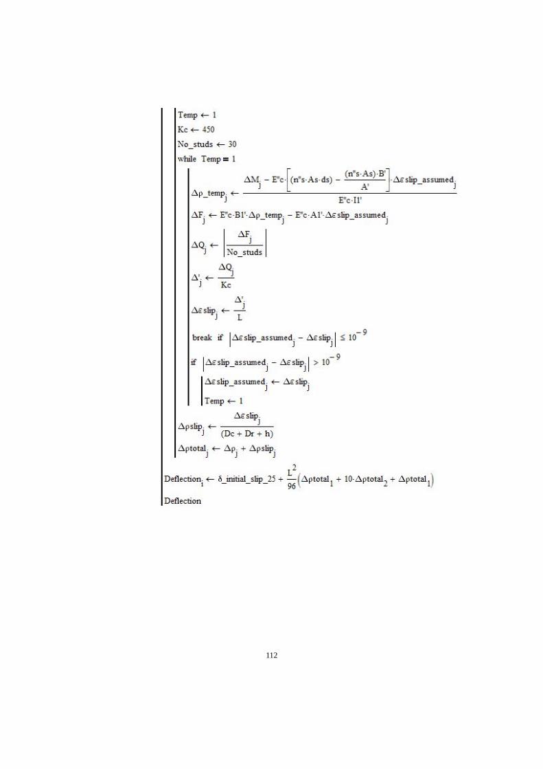
112

113

Step 3. Results

In summary,

114

Short- and long-term mid-span deflection for the W21x55 at 32 ft. for 25% interaction

Short-term Long-term (after 250 days)

Mid-span deflection

(unit : inches) 0.70 1.157

Immediate deflection limitation check (Maximum permissible deflection = L/360)

1.067360

Lin > 0.70 in. (O.K.)

Deflection limitation check after 250 days

1.067360

Lin <1.157 in. (N.G.)

The ratio of the long-term and short-term deflection

1.157 .1.653

0.70 .long term

short term

in

in

Similarly, the final values can be obtained throughout the above procedure when other creep and shrinkage values are used, and the results can be summarized as follow.

Long-term deflection The ratio of the long- and short-term deflection

Colored values indicate that its long-term deflection exceeds the maximum allowable deflection.