CrimeStat Version 3.3 Update Notes: Part I: Fixes Getis-Ord G Bayesian Journey-to-Crime Ned Levine Ned Levine & Associates Houston, TX

July 2010

The author would like to thank Ms. Haiyan Teng and Mr. Pradeep Mohan for the programming and Dr. Dick1

Block of Loyola University for reading and editing the update notes. Mr. Ron Wilson of the NationalInstitute of Justice deserves thanks for overseeing the project and Dr. Shashi Shekhar of the University ofMinnesota is thanked for supervising some of the programming. Additional thanks should be given to Dr.David Wong for help with the Getis-Ord ‘G’ and local Getis-Ord and Dr. Wim Bernasco, Dr. MichaelLeitner, Dr. Craig Bennell, Dr. Brent Snook, Dr. Paul Taylor, Dr. Josh Kent, and Ms. Patsy Lee forextensively testing the Bayesian Journey to Crime module.

CrimeStat Version 3.3 Update Notes: Part I: Fixes Getis-Ord G Bayesian Journey-to-Crime

July 2010

Ned Levine1

Ned Levine & AssociatesHouston, TX

This is Part I in the update notes for version 3.3 They provide information on some of thechanges to CrimeStat III since the release of version 3.0 in March 2005. They incorporate the changesthat were included in version 3.1, which was released in March 2007 and version 3.2 that was released inJune 2009, and re-released in September 2009.

The notes proceed by, first, discussing changes that were made to the existing routines fromversion 3.0 and, second, by discussing some new routines and organizational changes that were madesince version 3.0 (either in version 3.1 or in this current version, 3.2). For all existing routines, thechapters of the CrimeStat manual should be consulted. Part II of the update notes to version 3.3discusses the new regression module.

2

Table of Contents

Known Problems with Version 3.2Accessing the Help Menu in Windows Vista 5Running CrimeStat with MapInfo Open 5

Fixes and Improvements to Existing Routines from Version 3.0 5Paths 5MapInfo Output 5Geometric Mean 6

Uses 7

Harmonic Mean 7Uses 7

Linear Nearest Neighbor Index 8Risk-adjusted Nearest Neighbor Hierarchical Clustering 8Crime Travel Demand Module 8Crime Travel Demand Project Directory Utility 9Moran Correlogram 9

Calculate for Individual Intervals 9

Simulation of Confidence Intervals for Anselin’s Local Moran 9Example of Simulated Confidence Interval for Local Moran Statistic 10Simulated vs. Theoretical Confidence Intervals 13Potential Problem with Significance Tests of Local “I” 14

New Routines Added in Versions 3.1 through 3.3 14Spatial Autocorrelation Tab 14Getis-Ord “G” Statistic 14

Testing the Significance of G 15Simulating Confidence Intervals for G 17Running the Getis-Ord “G” 17Search distance 17Output 17Getis-Ord simulation of confidence intervals 18Example 1: Testing Simulated Data with the Getis-Ord “G” 18Example 2: Testing Houston Burglaries with the Getis-Ord “G” 22Use and limitations of the Getis-Ord “G” 23

Geary Correlogram 24Adjust for Small Distances 24Calculate for Individual Intervals 24Geary Correlogram Simulation of Confidence Intervals 24Output 24Graphing the “C” Values by Distance 25Example: Testing Houston Burglaries with the Geary Correlogram 25Uses of the Geary Correlogram 27

3

Getis-Ord Correlogram 27Getis-Ord Simulation of Confidence Intervals 27Output 27Graphing the “G” Values by Distance 28Example: Testing Houston Burglaries with the Getis-Ord Correlogram 28Uses of the Getis-Ord Correlogram 28

Getis-Ord Local “G” 30ID Field 31Search Distance 31Getis-Ord Local “G” Simulation of Confidence Intervals 31Output for Each Zone 31Example: Testing Houston Burglaries with the Getis-Ord Local “G” 32Uses of the Getis-Ord Local “G” 32Limitations of the Getis-Ord Local “G” 32

Interpolation I and II Tabs 34Head Bang 34

Rates and Volumes 35Decision Rules 35Example to Illustrate Decision Rules 37Setup 39Output 41Example 1: Using the Head Bang for Mapping Houston Burglaries 41Example 2: Using the Head Bang for Mapping Houston Burglary Rates 41Example 3: Using the Head Bang for Creating Burglary Rates 44Uses of the Head Bang Routine 47Limitations of the Head Bang Routine 47

Interpolated Head Bang 47Method of Interpolation 47Choice of Bandwidth 48Output (areal) Units 48Calculate Densities or Probabilities 48Output 49Example: Using the Interpolated Head Bang to Visualize Houston Burglaries 49Advantages and Disadvantages of the Interpolated Head Bang 49

Bayesian Journey to Crime Module 52Bayesian Probability 52Bayesian Inference 54Application of Bayesian Inference to Journey to Crime Analysis 55

The Bayesian Journey to Crime Estimation Module 60Data Preparation for Bayesian Journey to Crime Estimation 60Logic of the Routine 64

Bayesian Journey to Crime Diagnostics 65Data Input 65Methods Tested 65Interpolated Grid 66Output 67Which is the Most Accurate and Precise Journey to Crime Estimation Method? 68

4

Measures of Accuracy and Precision 69Testing the Routine with Serial Offenders from Baltimore County 75Conclusion of the Evaluation 78Tests with Other Data Sets 79

Estimate Likely Origin of a Serial Offender 79Data Input 80Selected Method 80Interpolated Grid 80Output 81Accumulator Matrix 81Two Examples of Using the Bayesian Journey to Crime Routine 82Potential to Add more Information to Improve the Methodology 92Probability Filters 95Summary 95

References 96

5

Known Problems with Version 3.2a

There are several known problems with version 3.2a.

Accessing the Help Menu in Windows Vista

CrimeStat III works with the Windows Vista operating system. There are several problems thathave been identified with Vista, however. First, Vista does not recognize the help menu. If a user clickson the help menu button in CrimeStat, there will be no response. However, Microsoft has developed aspecial file that allows help menus to be viewed in Vista. It will be necessary for Vista users to obtain thefile and install it according the instructions provided by Microsoft. The URL is found at:

http://support.microsoft.com/kb/917607

Second, version 3.2 has problems running multiple Monte Carlo simulations in Vista. CrimeStatis a multi-threading routine, which means that it will run separate calculations as unique ‘threads’. Ingeneral, this capability works with Vista. However, if multiple Monte Carlo simulations are run,“irrecoverable error” messages are produced with some of the results not being visible on the outputscreen. Since version 3.2a added a number of new Monte Carlo simulations (Getis-Ord “G”, GearyCorrelogram, Getis-Ord Correlogram, Anselin’s Local Moran, and Getis-Ord Local “G”), there is apotential for this error to become more prominent. This is a Vista problem only and involves conflictsover access to the graphics device interface. The output will not be affected and the user can access the‘graph’ button for those routines where it is available. We suggest that users run only one simulation at atime. This problem does not occur when the program is run in Windows XP. We have tested it in theWindows 7 Release Candidate and the problem appears to have been solved.

Running CrimeStat with MapInfo Open

The same ‘dbf’ or ‘tab’ file should not be opened simultaneously in MapInfo and CrimeStat. ®

This causes a file conflict error which may cause CrimeStat to crash. This is not a problem withArcGIS .®

Fixes and Improvements to Version 3.0

The following fixes and improvements to version 3.0 have been made.

Paths

For any output file, the program now checks that a path which is defined actually exists.

MapInfo Output

The output format for MapInfo MIF/MID files has been updated. The user can access a varietyof common projections and their parameters. MapInfo uses a file called MAPINFOW.PRJ, which is inthe MapInfo application folder, that lists many projections and their parameter. New projections can alsobe added to that file; users should consult the MapInfo Interchange documentation file. To use the

6

projections in CrimeStat copy the file (MAPINFOW.PRJ) to the same directory that CrimeStat resideswithin. When this is done, CrimeStat will allow the user to scroll down and select a particular projectionthat will then be saved in MIF/MID format for graphical output. The user can also choose to define acustom projection by filling in the eight parameter fields that are required: name of projection (optional),projection number, datum number, units, origin longitude, origin latitude, scale factor, false easting, andfalse northing. We suggest that any custom projection be added to the MAPINFOW.PRJ file. Note thatthe first projection listed in the file ("--- Longitude / Latitude ---") has one too many zeros and won’t beread. Use the second definition or remove one zero from that first line.

Geometric Mean

The Geometric Mean output in the “Mean center and standard distance” routine under SpatialDescription now allows weighted values. It is defined as (Wikipedia, 2007a):

N

iGeometric Mean of X = GM(X) = Ð ( X ) (Up. 1.1)Wi 1/(ÓWi)

i=1

N

iGeometric Mean of Y = GM(Y) = Ð (Y ) (Up. 1.2)Wi 1/(ÓWi)

i=1

where Ð is the product term of each point value, i (i.e., the values of X or Y are multiplied times each

iother), W is the weight used (default=1), and N is the sample size (Everitt, 1995). The weights have tobe defined on the Primary File page, either in the Weights field or in the Intensity field (but not bothtogether).

The equation can be evaluated by logarithms.

i i1 G[W *Ln(X )]

1 1 2* 2 2* NLn[GM(X)] = ---- [ W *Ln(X ) + W Ln(X ) + ..+ W Ln(X ) ] = ------------------ (Up. 1.3)

i i GW GW

i i 1 G[W *Ln(Y )]

1 1 2* 2 2* NLn[GM(Y)] = ---- [ W *Ln(Y ) + W Ln(Y ) + ..+ W Ln(Y ) ] = ---------------------- (Up. 1.4)

i i GW GW

GM(X) = e (Up. 1.5)Ln[GM(X)]

GM(Y) = e (Up.1.6)Ln[GM(Y)]

The geometric mean is the anti-log of the mean of the logarithms. If weights are used, then thelogarithm of each X or Y value is weighted and the sum of the weighted logarithms are divided by thesum of the weights. If weights are not used, then the default weight is 1 and the sum of the weights willequal the sample size. The geometric mean is output as part of the Mcsd routine and has a ‘Gm’ prefixbefore the user defined name.

7

Uses

The geometric mean is used when units are multipled by each other (e.g., a stock’s valueincreases by 10% one year, 15% the next, and 12% the next) (Wikipedia, 2007a). One can’t just take thesimple mean because there is a cumulative change in the units. In most cases, this is not relevant to point(incident) locations since the coordinates of each incident are independent and are not multiplied by eachother. However, the geometric mean can be useful because it first converts all X and Y coordinates intologarithms and, thus, has the effect of discounting extreme values.

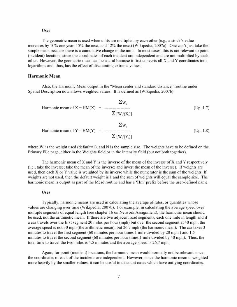
Harmonic Mean

Also, the Harmonic Mean output in the “Mean center and standard distance” routine underSpatial Description now allows weighted values. It is defined as (Wikipedia, 2007b):

i GWHarmonic mean of X = HM(X) = ------------------- (Up. 1.7)

i i G [W /(X )]

i GWHarmonic mean of Y = HM(Y) = ------------------- (Up. 1.8)

i iG [W /(Y )]

iwhere W is the weight used (default=1), and N is the sample size. The weights have to be defined on thePrimary File page, either in the Weights field or in the Intensity field (but not both together).

The harmonic mean of X and Y is the inverse of the mean of the inverse of X and Y respectively(i.e., take the inverse; take the mean of the inverse; and invert the mean of the inverse). If weights areused, then each X or Y value is weighted by its inverse while the numerator is the sum of the weights. Ifweights are not used, then the default weight is 1 and the sum of weights will equal the sample size. Theharmonic mean is output as part of the Mcsd routine and has a ‘Hm’ prefix before the user-defined name.

Uses

Typically, harmonic means are used in calculating the average of rates, or quantities whosevalues are changing over time (Wikipedia, 2007b). For example, in calculating the average speed overmultiple segments of equal length (see chapter 16 on Network Assignment), the harmonic mean shouldbe used, not the arithmetic mean. If there are two adjacent road segments, each one mile in length and ifa car travels over the first segment 20 miles per hour (mph) but over the second segment at 40 mph, theaverage speed is not 30 mph (the arithmetic mean), but 26.7 mph (the harmonic mean). The car takes 3minutes to travel the first segment (60 minutes per hour times 1 mile divided by 20 mph ) and 1.5minutes to travel the second segment (60 minutes per hour times 1 mile divided by 40 mph). Thus, thetotal time to travel the two miles is 4.5 minutes and the average speed is 26.7 mph.

Again, for point (incident) locations, the harmonic mean would normally not be relevant sincethe coordinates of each of the incidents are independent. However, since the harmonic mean is weightedmore heavily by the smaller values, it can be useful to discount cases which have outlying coordinates.

8

Linear Nearest Neighbor Index

The test statistic for the Linear Nearest Neighbor index on the Distance Analysis I page nowgives the correct probability level.

Risk-adjusted Nearest Neighbor Hierarchical Clustering (Rnnh)

The intensity checkbox for using the Intensity variable on the Primary File in calculating baselinevariable for the risk-adjusted nearest neighbor hierarchical clustering (Rnnh) has been brought from therisk parameters dialogue to the main interface. Some users had forgotten to check this box to utilize theintensity variable in the calculation.

Crime Travel Demand Module

Several fixes have been made to the Crime Travel Demand module routines:

1. In the “Make prediction” routine under the Trip Generation module of the Crime TravelDemand model, the output variable has been changed from “Prediction” to“ADJORIGINS” for the origin model and “ADJDEST” for the destination model.

2. In the “Calculate observed origin-destination trips” routine under the “Describe origin-destination trips” of the Trip Distribution module of the Crime Travel Demand model,the output variable is now called “FREQ”.

3. Under the “Setup origin-destination model” page of the Trip Distribution module of theCrime Travel Demand, there is a new parameter defining the minimum number of tripsper cell. Typically, in the gravity model, many cells will have small predicted values(e.g., 0.004). In order to concentrate the predicted values, the user can set a minimumlevel. If the predicted value is below this minimum, the routine automatically sets a zero(0) value with the remaining predicted values being re-scaled so that the total number ofpredicted trips remains constant. The default value is 0.05.

This parameter should be used cautiously, however, as extreme concentration can occurby merely raising this value. Because the number of predicted trips remains constant,setting a minimum that is too high will have the effect of increasing all values greaterthan the minimum substantially. For example, in one run where the minimum was set at5, a re-scaled minimum value for a line became 13.3.

4. For the Network Assignment routine, the prefix for the network load output is now VOL.

5. In defining a travel network either on the Measurement Parameters page or on theNetwork Assignment page, if the network is defined as single directional, then the “Fromone way flag” and “To one way flag” options are blanked out.

9

Crime Travel Demand Project Directory Utility

The Crime Travel Demand module is a complex model that involves many different files. Because of this, we recommend that the separate steps in the model be stored in separate directoriesunder a main project directory. While the user can save any file to any directory within the module,keeping the inputs and output files in separate directories can make it easier to identify files as well asexamine files that have already been used at some later time.

A new project directory utility tab under the Crime Travel Demand module allows the creation ofa master directory for a project and four separate sub-directories under the master directory thatcorrespond to the four modeling stages. The user puts in the name of a project in the dialogue box andpoints it to a particular drive and directory location (depending on the number of drives available to theuser). For example, a project directory might be called “Robberies 2003” or “Bank robberies 2005”. The utility then creates this directory if it does not already exist and creates four sub-directoriesunderneath the project directory:

Trip generationTrip distributionMode splitNetwork assignment

The user can then save the different output files into the appropriate directories. Further, foreach sequential step in the crime travel demand model, the user can easily find the output file from theprevious step which would then become the input file for the next step.

Moran Correlogram

Calculate for Individual Intervals

Currently, the Moran Correlogram calculates a cumulative value for the interval from a distanceof 0 up to the mid-point of the interval. If the option to calculate for individual intervals is checked, the“I” value will be calculated only for those pairs of points that are separated by a distance between theminimum and maximum distances of the interval (i.e., excluding distances that are shorter than theminimum value of the interval). This can be useful for checking the spatial autocorrelation for a specificinterval or checking whether some distances don’t have sufficient numbers of points (in which case the“I” value will be unreliable).

Simulation of Confidence Intervals for Anselin’s Local Moran

In previous versions of CrimeStat, the Anselin’s Local Moran routine had a option to calculatethe variance and a standardized “I” score (essentially, a Z-test of the significance of the “I” value). One problem with this test is that “I” may not actually follow a normal standard error. That is, if “I” iscalculated for all zones with random data, the distribution of the statistic may not be normally distributed.This would be especially true if the variable of interest, X, is a skewed variable with some zones havingvery high values while the majority having low values, as is typically true with crime distributions.

Consequently, the user can estimate the confidence intervals using a Monte Carlo simulation. Inthis case, a permutation type simulation is run whereby the original values of the intensity variable, Z,

10

are maintained but are randomly re-assigned for each simulation run. This will maintain the distributionof the variable Z but will estimate the value of I for each under random assignment of this variable. Note: a simulation may take time to run especially if the data set is large or if a large number ofsimulation runs are requested.

If a permutation Monte Carlo simulation is run to estimate confidence intervals, specify thenumber of simulations to be run (e.g., 1000, 5,000, 10000). In addition to the above statistics, the outputof includes the results that were obtained by the simulation for:

1. The minimum “I” value2. The maximum “I” value3. The 0.5 percentile of “I”4. The 2.5 percentile of “I”5. The 97.5 percentile of “I”6. The 99.5 percentile of “I”

The two pairs of percentiles (2.5 and 97.5; 0.5 and 99.5) create approximate 95% and 99%confidence intervals respectively. The minimum and maximum “I” values create an ‘envelope’ aroundeach zone. It is important to run enough simulations to produce reliable estimates.

The tabular results can be printed, saved to a text file or saved as a '.dbf' file with a LMoran<rootname> prefix with the root name being provided by the user. For the latter, specify a file name in the“Save result to” in the dialogue box. The ‘dbf’ file can then be linked to the input ‘dbf’ file by using theID field as a matching variable. This would be done if the user wants to map the “I” variable, the Z-test,or those zones for which the “I” value is either higher than the 97.5 or 99.5 percentiles or lower than the2.5 or 0.5 percentiles of the simulation results.

Example of Simulated Confidence Intervals for Local Moran Statistic

To illustrate the simulated confidence intervals, we apply Anselin’s Local Moran to an analysisof 2006 burglaries in the City of Houston. The data are 26,480 burglaries that have been aggregated to1,179 traffic analysis zones (TAZ). These are, essentially, census blocks or aggregations of censusblocks. Figure Up. 1.1 shows a map of burglaries in the City of Houston in 2006 by TAZ.

Anselin’s Local Moran statistic was calculated on each of 1,179 traffic analysis zones with 1,000Monte Carlo simulations being calculated. Figure Up. 1.2 shows a map of the calculated local “I” values. It can be seen that there are many more zones of negative spatial autocorrelation where the zones aredifferent than their neighbors. In most of these cases, the zone has no burglaries whereas it is surroundedby zones that have some burglaries. A few zones have positive spatial autocorrelation. In most of thecases, the zones have many burglaries and are surrounded by other zones with many burglaries.

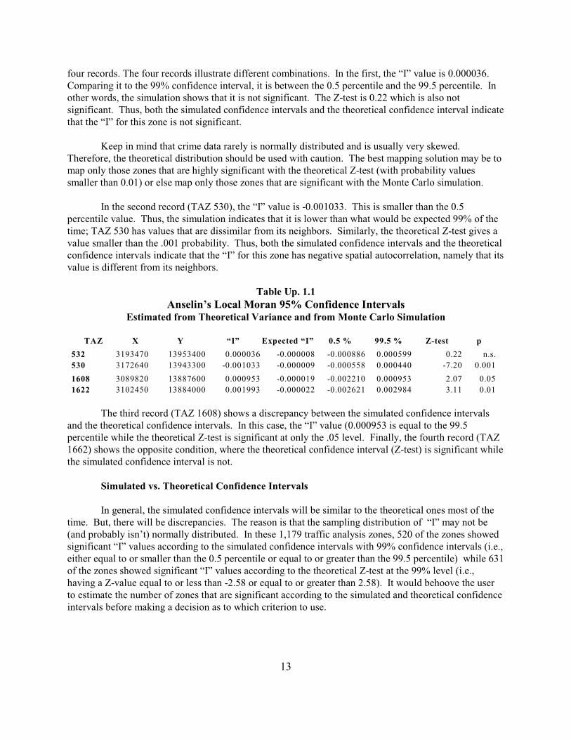
Confidence intervals were calculated in two ways. First, the theoretical variance was calculatedand a Z-test computed. This is done in CrimeStat by checking the ‘theoretical variance’ box. The testassumes that “I” is normally distributed. Second, a Monte Carlo simulation was used to estimate the99% confidence intervals (i.e., outside the 0.5 and 99.5 percentiles). Table Up. 1.1 shows the results for

Figure Up. 1.1:

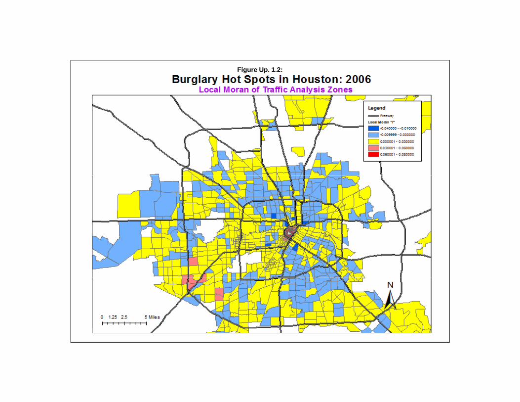
Figure Up. 1.2:

13

four records. The four records illustrate different combinations. In the first, the “I” value is 0.000036. Comparing it to the 99% confidence interval, it is between the 0.5 percentile and the 99.5 percentile. Inother words, the simulation shows that it is not significant. The Z-test is 0.22 which is also notsignificant. Thus, both the simulated confidence intervals and the theoretical confidence interval indicatethat the “I” for this zone is not significant.

Keep in mind that crime data rarely is normally distributed and is usually very skewed. Therefore, the theoretical distribution should be used with caution. The best mapping solution may be tomap only those zones that are highly significant with the theoretical Z-test (with probability valuessmaller than 0.01) or else map only those zones that are significant with the Monte Carlo simulation.

In the second record (TAZ 530), the “I” value is -0.001033. This is smaller than the 0.5percentile value. Thus, the simulation indicates that it is lower than what would be expected 99% of thetime; TAZ 530 has values that are dissimilar from its neighbors. Similarly, the theoretical Z-test gives avalue smaller than the .001 probability. Thus, both the simulated confidence intervals and the theoreticalconfidence intervals indicate that the “I” for this zone has negative spatial autocorrelation, namely that itsvalue is different from its neighbors.

Table Up. 1.1

Anselin’s Local Moran 95% Confidence IntervalsEstimated from Theoretical Variance and from Monte Carlo Simulation

TAZ X Y “I” Expected “I” 0.5 % 99.5 % Z-test p

532 3193470 13953400 0.000036 -0.000008 -0.000886 0.000599 0.22 n.s.

530 3172640 13943300 -0.001033 -0.000009 -0.000558 0.000440 -7.20 0.001

1608 3089820 13887600 0.000953 -0.000019 -0.002210 0.000953 2.07 0.05

1622 3102450 13884000 0.001993 -0.000022 -0.002621 0.002984 3.11 0.01

The third record (TAZ 1608) shows a discrepancy between the simulated confidence intervalsand the theoretical confidence intervals. In this case, the “I” value (0.000953 is equal to the 99.5percentile while the theoretical Z-test is significant at only the .05 level. Finally, the fourth record (TAZ1662) shows the opposite condition, where the theoretical confidence interval (Z-test) is significant whilethe simulated confidence interval is not.

Simulated vs. Theoretical Confidence Intervals

In general, the simulated confidence intervals will be similar to the theoretical ones most of thetime. But, there will be discrepancies. The reason is that the sampling distribution of “I” may not be(and probably isn’t) normally distributed. In these 1,179 traffic analysis zones, 520 of the zones showedsignificant “I” values according to the simulated confidence intervals with 99% confidence intervals (i.e.,either equal to or smaller than the 0.5 percentile or equal to or greater than the 99.5 percentile) while 631of the zones showed significant “I” values according to the theoretical Z-test at the 99% level (i.e.,having a Z-value equal to or less than -2.58 or equal to or greater than 2.58). It would behoove the userto estimate the number of zones that are significant according to the simulated and theoretical confidenceintervals before making a decision as to which criterion to use.

14

Potential Problem with Significance Tests of Local “I”

Also, one has to be suspect about a technique that finds significance in more than half the cases. It would probably be more conservative to use the 99% confidence intervals as a test for identifyingzones that show positive or negative spatial autocorrelation rather than using the 95% confidenceintervals or, better yet, choosing only those zones that have very negative or very positive “I” values. Unfortunately, this characteristic of the Anselin’s local Moran is also true of the local Getis-Ord routine(see below). The significance tests, whether simulated or theoretical, are not strict enough and, thereby,increase the likelihood of a Type I (false positive) error. A user must be careful in interpreting the “I”values for individual zones and would be better served choosing only the very highest or very lowest.

New Routines Added in Versions 3.1 through 3.2

New routines were added in versions 3.1 and 3.2. The second update chapter describes theregression routines that were added in version 3.3.

Spatial Autocorrelation Tab

Spatial autocorrelation tests have now been separated from the spatial distribution routines. Thissection now includes six tests for global spatial autocorrelation:

1. Moran’s “I” statistic2. Geary’s “C” statistic3. Getis-Ord “G” statistic (NEW)4. Moran Correlogram5. Geary Correlogram (NEW)6. Getis-Ord Correlogram (NEW)

These indices would typically be applied to zonal data where an attribute value can be assignedto each zone. Six spatial autocorrelation indices are calculated. All require an intensity variable in thePrimary File.

Getis-Ord “G” Statistic

The Getis-Ord “G” statistic is an index of global spatial autocorrelation for values that fall withina specified distance of each other (Getis and Ord, 1992). When compared to an expected value of “G”under the assumption of no spatial association, it has the advantage over other global spatialautocorrelation measures (Moran, Geary) in that it can distinguish between ‘hot spots’ and ‘cold spots’,which neither Moran’s “I” nor Geary’s “C” can do.

The “G” statistic calculates the spatial interaction of the value of a particular variable in a zonewith the values of that same variable in nearby zones, similar to Moran’s “I” and Geary’s “C”. Thus, it isalso a measure of spatial association or interaction. Unlike the other two measures, it only identifiespositive spatial autocorrelation, that is where zones have similar values to their neighbors. It cannotdetect negative spatial autocorrelation where zones have different values to their neighbors. But, unlikethe other two global measures it can distinguish between positive spatial autocorrelation where zoneswith high values are near to other zones with high values (high positive spatial autocorrelation) from

15

positive spatial autocorrelation which results from zones with low values being near to other zones alsowith low values (low positive spatial autocorrelation. Further, the “G” value is calculated with respect toa specified search distance (defined by the user) rather than to an inverse distance, as with the Moran’s“I” or Geary’s “C”.

The formulation of the general “G” statistic presented here is taken from Lee and Wong (2001). It is defined as:

i j j i j G G W (d) X X

G(d) = --------------------------------- (Up. 1.9)

ji i jG G X X

for a variable, X. This formula indicates that the cross-product of the value of X at location “i” and at

janother zone “j” is weighted by a distance weight, w (d) which is defined by either a ‘1' if the two zonesare equal to or closer than a threshold distance, d, or “0" otherwise. The cross-product is summed for allother zones, j, over all zones, i. Thus, the numerator is a sub-set of the denominator and can varybetween 0 and 1. If the distance selected is too small so that no other zones are closer than this distance,then the weight will be 0 for all cross-products of variable X. Hence, the value of G(d) will be 0. Similarly, if the distance selected is too large so that all other zones are closer than this distance, then theweight will be 1 for all cross-products of variable X. Hence, the value of G(d) will be 1.

There are actually two G statistics. The first one, G*, includes the interaction of a zone withitself; that is, zone “i” and zone “j” can be the same zone. The second one, G, does not include theinteraction of a zone with itself. In CrimeStat, we only include the G statistic (i.e., there is no interactionof a zone with itself) because, first, the two measures produce almost identical results and, second, theinterpretation of G is more straightforward than with G*. Essentially, with G, the statistic measures theinteraction of a zone with nearby zones (a ‘neighborhood’). See articles by Getis & Ord (1992) and byKhan, Qin and Noyce (2006) for a discussion of the use of G*.

Testing the Significance of G

By itself, the G statistic is not very meaningful. Since it can vary between 0 and 1, as thethreshold distance increases, the statistic will always approach 1.0. Consequently, G is compared to anexpected value of G under no significant spatial association. The expected G for a threshold distance, d,is defined as:

WE[G(d)] = ------------ (Up.1.10)

N(N-1)

where W is the sum of weights for all pairs and N is the number of cases. The sum of the weights isbased on symmetrical distances for each zone “i”. That is, if zone 1 is within the threshold distance ofzone 2, then zone 1 has a weight of 1 with zone 2. In counting the total number of weights for zone 1, theweight of zone 2 is counted. Similarly, zone 2 has a weight of 1 with zone 1. So, in counting the totalnumber of weights for zone 2, the weight of zone 1 is counted, too. In other words, if two zones arewithin the threshold (search) distance, then they both contribute 2 to the total weight.

16

Note that, since the expected value of G is a function of the sample size and the sum of weightswhich, in turn, is a function of the search distance, it will be the same for all variables of a single data setin which the same search distance is specified. However, as the search distance changes, so will theexpected G change.

Theoretically, the G statistic is assumed to have a normally distributed standard error. If this isthe case (and we often don’t know if it is), then the standard error of G can be calculated and a simplesignificance test based on the normal distributed be constructed. The variance of G(d) is defined as:

Var[G(d)] = E(G ) - E(G) (Up. 1.11)2 2

where

1

o 2 1 4 2 1 2 3 1 3 4 1E(G) = -------------------- [B m + B m + B m m + B m m + B m ] (Up. 1.12)2 2 2 4

1 2 (m - m ) n2 2 (4)

and where

j1 im = G X (Up. 1.13)

j2 im = G X (Up. 1.14)2

3 im = GX (Up. 1.15)3

4 im = GX (Up. 1.16)4

n = n(n-1)(n-2)(n-3) (Up. 1.17)(4)

i j1 ij jiS = 0.5 G G (w +w ) (Up. 1.18)2

i j j2 ij jiS = G (G w + G w ) (Up. 1.19)2

0 1 2B = (n - 3n + 3)S - nS + 3W (Up. 1.20)2 2

1 1 2B = -[(n - n)S - 2nS + 3W ] (Up. 1.21)2 2

2 1 2B = -[2nS - (n+3)S + 6W ] (Up. 1.22)2

3 1 2B = 4(n - 1)S - 2(n + 1)S + 8W (Up. 1.23)2

4 1 2B = S -S + W (Up. 1.24)2

where i is the zone being calculated, j is all other zones, and n (Lee and Wong, 2001). Note that thisformula is different than that written in other sources (e.g., see Lees, 2006) but is consistent with theformulation by Getis and Ord (1992).

The standard error of G(d) is the square root of the variance of G. Consequently, a Z-test can beconstructed by:

S.E.[G(d)] = SQRT{Var[G(d)]} (Up. 1.25)

G(d) - E[G(d)]Z[G(d)] = --------------------------- (Up. 1.26)

S.E.[G(d)]

17

Relative to the expected value of G, a positive Z-value indicates spatial clustering of high values(high positive spatial autocorrelation or ‘hot spots’) while a negative Z-value indicates spatial clusteringof low values (low positive spatial autocorrelation or ‘cold spots’). A “G” value around 0 typicallyindicates either no positive spatial autocorrelation, negative spatial autocorrelation (which the Getis-Ordcannot detect), or that the number of ‘hot spots’ more or less balances the number of ‘cold spots’. Notethat the value of this test will vary with the search distance selected. One search distance may yield asignificant spatial association for G whereas another may not. Thus, the statistic is useful for identifyingdistances at which spatial autocorrelation exists (see the Getis-Ord Correlogram below).

Also, and this is an important point, the expected value of G as calculated in equation Up.1.10 isonly meaningful if the variable is positive. For variables with negative values, such as residual errorsfrom a regression model, one cannot use equation Up. 1.10 but, instead, must use a simulation to estimateconfidence intervals.

Simulating Confidence Intervals for G

One of the problems with this test is that G may not actually follow a normal standard error. That is, if G was calculated for a specific distance, d, with random data, the distribution of the statisticmay not be normally distributed. This would be especially true if the variable of interest, X, is a skewedvariable with some zones having very high values while the majority of zones having low values.

Consequently, the user has an alternative for estimating the confidence intervals using a MonteCarlo simulation. In this case, a permutation type simulation is run whereby the original values of theintensity variable, Z, are maintained but are randomly re-assigned for each simulation run. This willmaintain the distribution of the variable Z but will estimate the value of G under random assignment ofthis variable. The user can take the usual 95% or 99% confidence intervals based on the simulation.Keep in mind that a simulation may take time to run especially if the data set is large or if a large numberof simulation runs are requested.

Running the Getis-Ord “G” Routine

The Getis-Ord global “G” routine is found on the new Spatial Autocorrelation tab under the mainSpatial Description heading. The variable that will be used in the calculation is the intensity variablewhich is defined on the Primary File page. By choosing different intensity variables, the user canestimate G for different variables (e.g., number of assaults, robbery rate).

Search distance

The user must specify a search distance for the test and indicate the distance units (miles,nautical miles, feet, kilometers, or meters,).

Output

The Getis-Ord “G” routine calculates 7 statistics:

1. The sample size2. Getis-Ord “G”

18

3. The spatially random (expected) "G"4. The difference between “G” and the expected “G”5. The standard error of "G"6. A Z-test of "G" under the assumption of normality (Z-test)7. The one-tail probability level8. The two-tail probability level

Getis-Ord Simulation of Confidence Intervals

If a permutation Monte Carlo simulation is run to estimate confidence intervals, specify thenumber of simulations to be run (e.g., 100, 1000, 10000). In addition to the above statistics, the output ofincludes the results that were obtained by the simulation for:

1. The minimum “G” value2. The maximum “G” value3. The 0.5 percentile of “G”4. The 2.5 percentile of “G”5. The 5 percentile of “G”6. The 10 percentile of “G”7. The 90 percentile of “G”8. The 95 percentile of “G”9. The 97.5 percentile of “G”10. The 99.5 percentile of “G”

The four pairs of percentiles (10 and 90; 5 and 95; 2.5 and 97.5; 0.5 and 99.5) create approximate80%, 90%, 95% and 99% confidence intervals respectively.

The tabular results can be printed, saved to a text file or saved as a '.dbf' file. For the latter,specify a file name in the “Save result to” in the dialogue box.

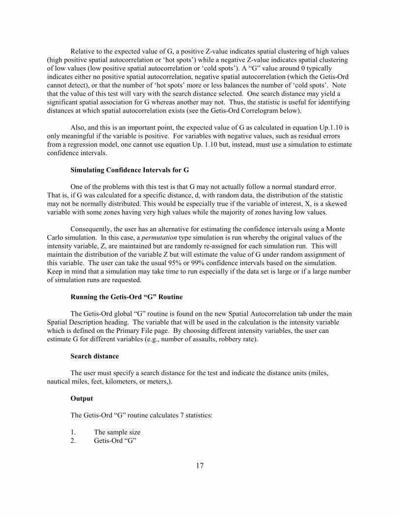
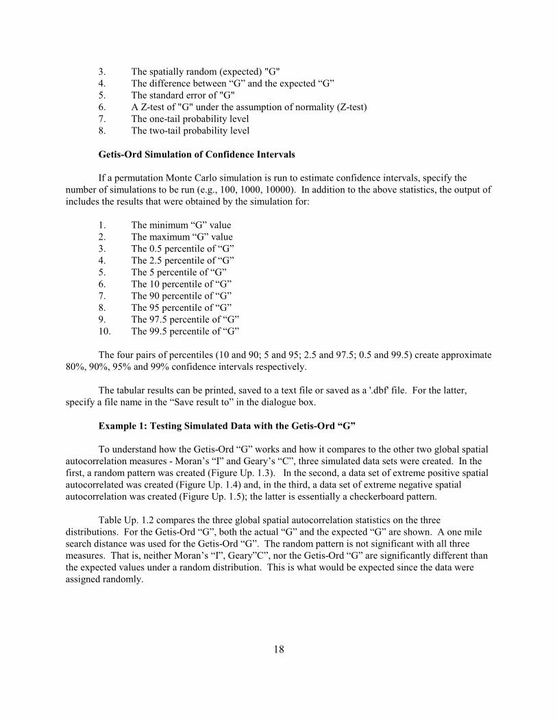
Example 1: Testing Simulated Data with the Getis-Ord “G”

To understand how the Getis-Ord “G” works and how it compares to the other two global spatialautocorrelation measures - Moran’s “I” and Geary’s “C”, three simulated data sets were created. In thefirst, a random pattern was created (Figure Up. 1.3). In the second, a data set of extreme positive spatialautocorrelated was created (Figure Up. 1.4) and, in the third, a data set of extreme negative spatialautocorrelation was created (Figure Up. 1.5); the latter is essentially a checkerboard pattern.

Table Up. 1.2 compares the three global spatial autocorrelation statistics on the threedistributions. For the Getis-Ord “G”, both the actual “G” and the expected “G” are shown. A one milesearch distance was used for the Getis-Ord “G”. The random pattern is not significant with all threemeasures. That is, neither Moran’s “I”, Geary”C”, nor the Getis-Ord “G” are significantly different thanthe expected values under a random distribution. This is what would be expected since the data wereassigned randomly.

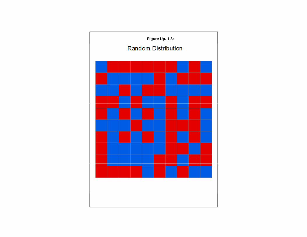
Figure Up. 1.3:

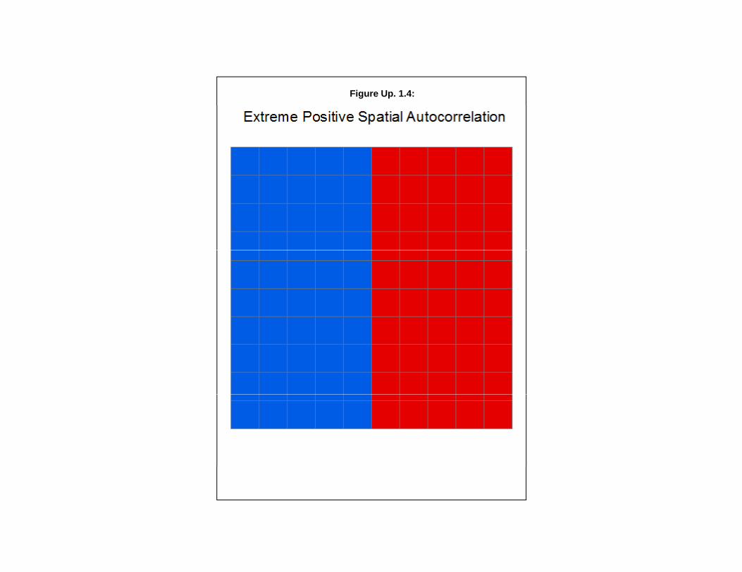
Figure Up. 1.4:

Figure Up. 1.5:

22

Table Up. 1.2:

Global Spatial Autocorrelation Statistics for Simulated Data SetsN = 100 Grid Cells

Pattern Moran’s “I” Geary’s “C” Getis-Ord “G” Expected “G” (1 mile search) (1 mile search)

Random -0.007162 0.965278 0.151059 0.159596n.s. n.s n.s

Positive spatialautocorrelation 0.292008 0.700912 0.241015 0.159596*** *** ***

Negative spatialautocorrelation -0.060071 1.049471 0.140803 0.159596*** * n.s.

_____________________n.s not significant* p#.05** p#.01*** p#.001

For the extreme positive spatial autocorrelation pattern, on the other hand, all three measuresshow highly significant differences with a random simulation. Moran’s “I” is highly positive. Geary’s“C is below 1.0, indicating positive spatial autocorrelation and the Getis-Ord “G” has a “G” value that issignificantly higher than the expected “G” according to the Z-test based on the theoretical standard error.The Getis-Ord “G”, therefore, indicates that the type of spatial autocorrelation is high positive. Finally,the extreme negative spatial autocorrelation pattern (Figure Up. 1.5 above) shows different results for thethree measures. Moran’s “I” shows negative spatial autocorrelation and is highly significant. Geary’s “Calso shows negative spatial autocorrelation but it is significant only at the .05 level. Finally, the Getis-Ord “G” is not significant which is not surprising since the statistic cannot detect negative spatialautocorrelation. The “G” is slightly smaller than the expected “G”, which indicates low positive spatialautocorrelation, but it is not significant.

In other words, all three statistics can identify positive spatial correlation. Of these, Moran’s “I”is a more powerful (sensitive) test than either Geary’s “C” or the Getis-Ord “G”. For the negative spatialautocorrelation pattern, only Moran’s “I” and Geary’s “C” is able to detect it and, again, Moran’s “I” ismore powerful than Geary’s “C”. On the other hand, only the Getis-Ord “G” can distinguish betweenhigh positive and low positive spatial autocorrelation. The Moran and Geary tests would show theseconditions to be identical, as the example below shows.

Example 2: Testing Houston Burglaries with the Getis-Ord “G”

Now, let’s take a real data set, the 26,480 burglaries in the City of Houston in 2006 aggregated to1,179 traffic analysis zones (Figure Up. 1.1 above). To compare the Getis-Ord “G” statistic with theMoran’s “I” and Geary’s “C”, the three spatial autocorrelation tests were run on this data set. The Getis-Ord “G” was tested with a search distance of 2 miles and 1000 simulation runs were made on the “G”. Table Up. 1.3 shows the three global spatial autocorrelation statistics for these data.

23

Table Up. 1.3:

Global Spatial Autocorrelation Statistics for City of Houston Burglaries: 2001N = 1,179 Traffic Analysis Zones

Moran’s “I” Geary’s “C” Getis-Ord “G” (2 mile search)

Observed 0.25179 0.397080 0.028816

Expected -.000849 1.000000 0.107760

Observed -Expected 0.25265 -0.60292 -0.07894

Standard Error 0.002796 0.035138 0.010355

Z-test 90.35 -17.158851 -7.623948

p-value *** *** ***

Based on simulation:2.5 percentile n.a. n.a. 0.088162

97.5 percentile n.a. n.a. 0.129304 _____________________n.s not significant* p#.05** p#.01*** p#.001

The Moran and Geary tests show that the Houston burglaries have significant positive spatialautocorrelation (zones have values that are similar to their neighbors). Moran’s “I” is significantlyhigher than the expected “I”. Geary’s “C” is significantly lower than the expected “C” (1.0), whichmeans positive spatial autocorrelation. However, the Getis-Ord “G” is lower than the expected “G valueand is significant whether using the theoretical Z-test or the simulated confidence intervals (notice howthe “G” is lower than the 2.5 percentile). This indicates that, in general, zones having low values arenearby other zones with low values. In other words, there is low positive spatial autocorrelation,suggesting a number of ‘cold spots’. Note also that the expected “G” is between the 2.5 percentile and97.5 percentile of the simulated confidence intervals.

Uses and Limitations of the Getis-Ord “G”

The advantage of the “G” statistic over the other two spatial autocorrelation measures is that itcan definitely indicate ‘hot spots’ or ‘cold spots’. The Moran and Geary measures cannot determinewhether the positive spatial autocorrelation is ‘high positive’ or ‘low positive’. With Moran’s “I” orGeary’s “C”, an indicator of positive spatial autocorrelation means that zones have values that are similarto their neighbors. However, the positive spatial autocorrelation could be caused by many zones withlow values being concentrated, too. In other words, one cannot tell from those two indices whether theconcentration is a hot spot or a cold spot. The Getis-Ord “G” can do this.

24

The main limitation of the Getis-Ord “G” is that it cannot detect negative spatial autocorrelation,a condition that, while rare, does occur. With the checkerboard pattern above (Figure Up. 1.5), this testcould not detect that there was negative spatial autocorrelation. For this condition (which is rare),Moran’s “I” or Geary’s “C” would be more appropriate tests.

Geary Correlogram

The Geary “C” statistic is already part of CrimeStat (see chapter 4 in the manual). This statistictypically varies between 0 and 2 with a value of 1 indicating no spatial autocorrelation. Values less than1 indicate positive spatial autocorrelation (zones have similar values to their neighbors) while valuesgreater than 1 indicate negative spatial autocorrelation (zones have different values from their neighbors).

The Geary Correlogram requires an intensity variable in the primary file and calculates the Geary“C” index for different distance intervals/bins. The user can select any number of distance intervals. Thedefault is 10 distance intervals. The size of each interval is determined by the maximum distance betweenzones and the number of intervals selected.

Adjust for Small Distances

If checked, small distances are adjusted so that the maximum weighting is 1 (see documentationfor details.) This ensures that the “C” values for individual distances won't become excessively large orexcessively small for points that are close together. The default value is no adjustment.

Calculate for Individual Intervals

The Geary Correlogram normally calculates a cumulative value for the interval/bin from adistance of 0 up to the mid-point of the interval/bin. If this option is checked, the “C” value will becalculated only for those pairs of points that are separated by a distance between the minimum andmaximum distances of the interval. This can be useful for checking the spatial autocorrelation for aspecific interval or checking whether some distance intervals don’t have sufficient numbers of points (inwhich case the “C” value will be unreliable for that distance).

Geary Correlogram Simulation of Confidence Intervals

Since the Geary’s “C” statistic may not be normally distributed, the significance test is frequentlyinaccurate. Instead, a permutation type Monte Carlo simulation is run whereby the original values of thevariable, Z, are maintained but are randomly re-assigned for each simulation run. This will maintain thedistribution of the variable Z but will estimate the value of “C” under random assignment of this variable. Specify the number of simulations to be run (e.g., 1000, 5000, 10000). Note, a simulation may take timeto run especially if the data set is large or if a large number of simulation runs are requested.

Output

The output includes:

1. The sample size2. The maximum distance

25

3. The bin (interval) number4. The midpoint of the distance bin5. The “C” value for the distance bin

and if a simulation is run:

6. The minimum “C” value for the distance bin7. The maximum “C” value for the distance bin8. The 0.5 percentile of “C” for the distance bin9. The 2.5 percentile of “C” for the distance bin10. The 97.5 percentile of “C” for the distance bin11. The 99.5 percentile of “C” for the distance bin.

The two pairs of percentiles (2.5 and 97.5; 0.5 and 99.5) create approximate 95% and 99%confidence intervals respectively. The minimum and maximum simulated “C” values create an‘envelope’ for each interval. However, unless a large number of simulations are run, the actual “C” valuemay fall outside the envelope for any one interval. The tabular results can be printed, saved to a text fileor saved as a '.dbf' file with a GearyCorr<root name> prefix with the root name being provided by theuser. For the latter, specify a file name in the “Save result to” in the dialogue box.

Graphing the “C” Values by Distance

A graph can be shown with the “C” value on the Y-axis by the distance bin on the X-axis. Clickon the “Graph” button. If a simulation is run, the 2.5 and 97.5 percentiles of the simulated “C” values arealso shown on the graph. The graph displays the reduction in spatial autocorrelation with distance. Thegraph is useful for selecting the type of kernel in the single- and dual-kernel interpolation routines whenthe primary variable is weighted (see Chapter 8 on Kernel Density Interpolation). For a presentationquality graph, however, the output file should be brought into Excel or another graphics program in orderto display the change in “C” values and label the axes properly.

Example: Testing Houston Burglaries with the Geary Correlogram

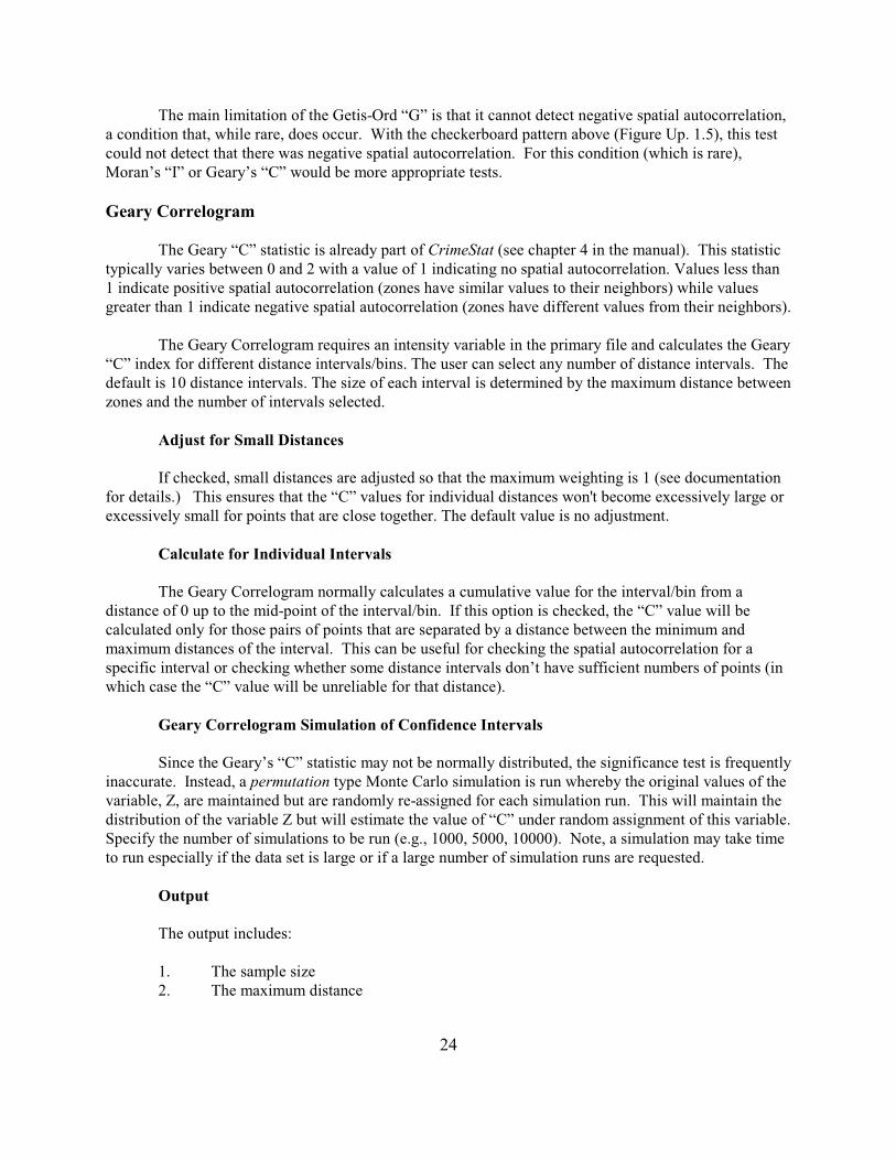
Using the same data set on the Houston burglaries as above, the Geary Correlogram was run with100 intervals (bins). The routine was also run with 1000 simulations to estimate confidence intervalsaround the “C” value. Figure Up. 1.6 illustrates the distance decay of “C” as a function of distance alongwith the simulated 95% confidence interval. The theoretical “C” under random conditions is also shown. As seen, the “C” values are below 1.0 for all distances tested and are also below the 2.5 percentilesimulated “C” for all intervals.

Thus, it is clear that there is substantial positive spatial autocorrelation with the Houstonburglaries. Looking at the ‘distance decay’, the “C” values decrease with distance indicating that theyapproach a random distribution. However, they level off at around 15 miles to the global “C” value(0.397). In other words, spatial autocorrelation is substantial in these data up to about a separation of 15miles, whereupon the general positive spatial autocorrelation holds. This distance can be used to setlimits for search distances in other routines (e.g., kernel density interpolation).

Figure Up. 1.6:

97.5 percentile of “C”

2 5 til f “C”

Theoretical random “C”

2.5 percentile of “C”

“C” of Houston burglaries

27

Uses of the Geary Correlogram

Similar to the Moran Correlogram and the Getis-Ord Correlogram (see below), the GearyCorrelogram is useful in order to determine the degree of spatial autocorrelation and how far away fromeach zone it typically lasts. Since it is an average over all zones, it is a general indicator of the spread ofthe spatial autocorrelation. This can be useful for defining limits to search distances in other routines,such as the single kernel density interpolation routine where a fixed bandwidth would be defined tocapture the majority of spatial autocorrelation.

Getis-Ord Correlogram

The Getis-Ord Correlogram calculates the Getis-Ord “G” index for different distanceintervals/bins. The statistic requires an intensity variable in the primary file and calculates the Getis-Ord“G” index for different distance intervals/bins. The user can select any number of distance intervals. Thedefault is 10 distance intervals. The size of each interval is determined by the maximum distance betweenzones and the number of intervals selected.

Getis-Ord Correlogram Simulation of Confidence Intervals

Since the Getis-Ord “G” statistic may not be normally distributed, the significance test isfrequently inaccurate. Instead, a permutation type Monte Carlo simulation is run whereby the originalvalues of the intensity variable, Z, are maintained but are randomly re-assigned for each simulation run. This will maintain the distribution of the variable Z but will estimate the value of G under randomassignment of this variable. Specify the number of simulations to be run (e.g., 100, 1000, 10000). Note,a simulation may take time to run especially if the data set is large or if a large number of simulation runsare requested.

Output

The output includes:

1. The sample size2. The maximum distance3. The bin (interval) number4. The midpoint of the distance bin5. The “G” value for the distance bin

and if a simulation is run, the simulated results under the assumption of random re-assignment for:

6. The minimum “G” value7. The maximum “G” value8. The 0.5 percentile of “G” 9. The 2.5 percentile of “G”10. The 97.5 percentile of “G”11. The 99.5 percentile of “G”

28

The two pairs of percentiles (2.5 and 97.5; 0.5 and 99.5) create approximate 95% and 99%confidence intervals respectively. The minimum and maximum “G” values create an ‘envelope’ for eachinterval. However, unless a large number of simulations are run, the actual “G” value for any intervalmay fall outside the envelope. The tabular results can be printed, saved to a text file or saved as a '.dbf'file with a Getis-OrdCorr<root name> prefix with the root name being provided by the user. For thelatter, specify a file name in the “Save result to” in the dialogue box.

Graphing the “G” Values by Distance

A graph can be shown that shows the “G” and Expected “G” values on the Y-axis by the distancebin on the X-axis. Click on the “Graph” button. If a simulation is run, the 2.5 and 97.5 percentile “G”values are also shown on the graph along with the “G”; the Expected “G” is not shown in this case. Thegraph displays the reduction in spatial autocorrelation with distance. Note that the “G” and expected “G”approach 1.0 as the search distance increases, that is as the pairs included within the search distanceapproximate the number of pairs in the entire data set. The graph is useful for selecting the type of kernelin the single- and dual-kernel interpolation routines when the primary variable is weighted (see Chapter 8on Kernel Density Interpolation). For a presentation quality graph, however, the output file should bebrought into Excel or another graphics program in order to display the change in “G” values and label theaxes properly.

Note that the “G” and expected “G” approach 1.0 as the search distance increases, that is as thepairs included within the search distance approximate the number of pairs in the entire data set. Graphingthe Getis-Ord correlogram is useful for selecting the type of kernel in the single- and dual-kernelinterpolation routines when the primary variable is weighted with an intensity value (see Chapter 8 onKernel Density Interpolation).

Example: Testing Houston Burglaries with the Getis-Ord Correlogram

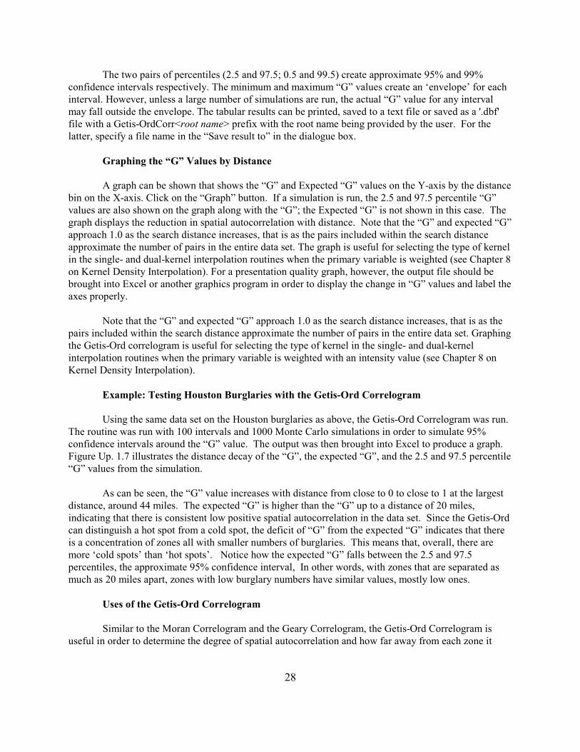
Using the same data set on the Houston burglaries as above, the Getis-Ord Correlogram was run.The routine was run with 100 intervals and 1000 Monte Carlo simulations in order to simulate 95%confidence intervals around the “G” value. The output was then brought into Excel to produce a graph.Figure Up. 1.7 illustrates the distance decay of the “G”, the expected “G”, and the 2.5 and 97.5 percentile“G” values from the simulation.

As can be seen, the “G” value increases with distance from close to 0 to close to 1 at the largestdistance, around 44 miles. The expected “G” is higher than the “G” up to a distance of 20 miles,indicating that there is consistent low positive spatial autocorrelation in the data set. Since the Getis-Ordcan distinguish a hot spot from a cold spot, the deficit of “G” from the expected “G” indicates that thereis a concentration of zones all with smaller numbers of burglaries. This means that, overall, there aremore ‘cold spots’ than ‘hot spots’. Notice how the expected “G” falls between the 2.5 and 97.5percentiles, the approximate 95% confidence interval, In other words, with zones that are separated asmuch as 20 miles apart, zones with low burglary numbers have similar values, mostly low ones.

Uses of the Getis-Ord Correlogram

Similar to the Moran Correlogram and the Geary Correlogram, the Getis-Ord Correlogram isuseful in order to determine the degree of spatial autocorrelation and how far away from each zone it

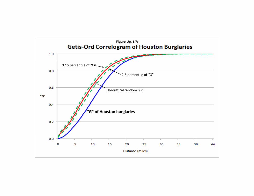
Figure Up. 1.7:

2.5 percentile of “G”

97.5 percentile of “G”

Theoretical random “G”

“G” f H b l i“G” of Houston burglaries

30

typically lasts. Since it is an average over all zones, it is a general indicator of the spread of the spatialautocorrelation. This can be useful for defining limits to search distances in other routines, such as thesingle kernel density interpolation routine or the MCMC spatial regression module (to be released inversion 4.0). Unlike the other two correlograms, however, it can distinguish hot spots from cold spots. Inthe example above, there are more cold spots than hot spots since the “G” is smaller than the expected“G” for most of the distances. The biggest limitation for the Getis-Ord Correlogram is that it cannotdetect negative spatial autocorrelation, where zones have different values from their neighbors. For thatcondition, which is rare, the other two correlograms should be used.

Getis-Ord Local “G”

The Getis-Ord Local G statistic applies the Getis-Ord "G" statistic to individual zones to assesswhether particular points are spatially related to the nearby points. Unlike the global Getis-Ord “G”, theGetis-Ord Local “G” is applied to each individual zone. The formulation presented here is taken fromLee and Wong (2001). The “G” value is calculated with respect to a specified search distance (definedby the user), namely:

j j j G w (d) X

iG(d) = ---------------------------- (Up. 1.27)

j jG X

i W

iE[G(d) ] = ------------ (Up. 1.28) (N-1)

ji * i j i i 1 W (n-1-W )*G X ) W (W - 1)2

iVar[G(d) ] = ---------------- * [----------------------------] + -------------- (Up. 1.29)

j j (G X ) (n-1)(n-2) (n-1)(n-2)2

j iwhere w is the weight of zone “j” from zone “i”, W is the sum of weights for zone “i”, and n is thenumber of cases.

The standard error of G(d) is the square root of the variance of G. Consequently, a Z-test can beconstructed by:

i iS.E.[G(d) ] = SQRT{Var[G(d) ]} (Up. 1.30)

i i G(d) - E[G(d) ]

iZ[G(d) ] = --------------------------- (Up. 1.31)

i S.E.[G(d) ]

31

A good example of using the Getis-Ord local “G” statistic in crime mapping is found in Chaineyand Racliffe (2005, pp. 164-172).

ID Field

The user should indicate a field for the ID of each zone. This ID will be saved with the outputand can then be linked with the input file (Primary File) for mapping.

Search Distance

The user must specify a search distance for the test and indicate the distance units (miles,nautical miles, feet, kilometers, meters,

Getis-Ord Local “G” Simulation of Confidence Intervals

Since the Getis-Ord “G” statistic may not be normally distributed, the significance test isfrequently inaccurate. Instead, a permutation type Monte Carlo simulation can be run whereby theoriginal values of the intensity variable, Z, for the zones are maintained but are randomly re-assigned tozones for each simulation run. This will maintain the distribution of the variable Z but will estimate thevalue of G for each zone under random assignment of this variable. Specify the number of simulations tobe run (e.g., 100, 1000, 10000).

Output for Each Zone

The output is for each zone and includes:

1. The sample size2. The ID for the zone3. The X coordinate for the zone4. The Y coordinate for the zone5. The “G” for the zone6. The expected “G” for the zone7. The difference between “G” and the expected “G”8. The standard deviation of “G” for the zone9. A Z-test of "G" under the assumption of normality for the zone

and if a simulation is run:

10. The 0.5 percentile of “G” for the zone11. The 2.5 percentile of “G” for the zone12. The 97.5 percentile of “G” for the zone13. The 99.5 percentile of “G” for the zone

The two pairs of percentiles (5 and 95; 2.5 and 97.5; 0.5 and 99.5) create approximate 95% and99% confidence intervals respectively around each zone. The minimum and maximum “G” values createan ‘envelope’ around each zone. However, unless a large number of simulations are run, the actual “G”value may fall outside the envelope for any zone. The tabular results can be printed, saved to a text file or

32

saved as a '.dbf' file. For the latter, specify a file name in the “Save result to” in the dialogue box. Thefile is saved with a LGetis-Ord<root name> prefix with the root name being provided by the user.

The ‘dbf’ output file can be linked to the Primary File by using the ID field as a matchingvariable. This would be done if the user wants to map the “G” variable, the expected “G”, the Z-test, orthose zones for which the “G” value is either higher than the 97.5 or 99.5 percentiles or lower than the2.5 or 0.5 percentiles of the simulation results respectively (95% or 99% confidence intervals).

Example: Testing Houston Burglaries with the Getis-Ord Local “G”

Using the same data set on the Houston burglaries as above, the Getis-Ord Local “G” was runwith a search radius of 2 miles and with 1000 simulations being run to produce 95% confidence intervalsaround the “G” value. The output file was then linked to the input file using the ID field to allow themapping of the local “G” values. Figure Up. 1.8 illustrates the local Getis-Ord “G” for different zones. The map displays the difference between the “G” and the expected “G (“G” minus expected “G”) withthe Z-test being applied to the difference. Zones with a Z-test of +1.96 or higher are shown in red (hotspots). Zones with Z-tests of -1.96 or smaller are shown in blue (cold spots) while zones with a Z-testbetween -1.96 and +1.96 are shown in yellow (no pattern).

As seen, there are some very distinct patterns of zones with high positive spatial autocorrelationand low positive spatial autocorrelation. Examining the original map of burglaries by TAZ (Figure Up.1.1 above), it can be seen that where there are a lot of burglaries, the zones show high positive spatialautocorrelation in Figure Up. 1.8. Conversely, where there are few burglaries, the zones show lowpositive spatial autocorrelation in Figure Up. 1.8.

Uses of the Getis-Ord Local “G”

The Getis-Ord Local “G” is very good at identifying hot spots and also good at identifying coldspots. As mentioned, Anselin’s Local Moran can only identify positive or negative spatialautocorrelation. Those zones with positive spatial autocorrelation could occur because zones with highvalues are nearby other zones with high values or zones with low values are nearby other zones with lowvalues. The Getis-Ord Local “G” can distinguish those two types.

Limitations of the Getis-Ord Local “G”

The biggest limitation with the Getis-Ord Local “G”, which applies to all the Getis-Ord routines,is that it cannot detect negative spatial autocorrelation, where a zone is surrounded by neighbors that aredifferent (either having a high value surrounded by zones with low values or having a low value andbeing surrounded by zones with high values). In actual use, both the Anselin’s Local Moran and theGetis-Ord Local “G” should be used to produce a full interpretation of the rsults.

Another limitation is that the significance tests are too weak, allowing too many zones to showsignificance. In the data shown in Figure Up. 1.8, more than half the zones (727) were statisticallysignificant, either by the Z-test or by the simulated 99% confidence intervals. Thus, there is a substantialType I error with this statistic (false positives), a similarity it shares with Anselin’s Local Moran. A usershould be careful in interpreting zones with significant “G” values and would probably be better servedby choosing only those zones with the highest or lowest “G” values.

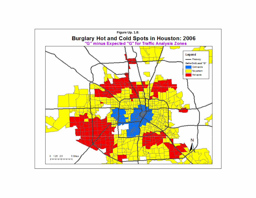
Figure Up. 1.8:

The Head Bang statistic is sometimes written as Head-Bang or even Headbang. We prefer to use the term2

without the hyphen.

34

Interpolation I and Interpolation II Tabs

The Interpolation tab, under Spatial Modeling, has now been separated into two tabs:Interpolation I and Interpolation II. The Interpolation I tab includes the single and dual kernel densityroutines that have been part of CrimeStat since version 1.0. The interpolation II tab includes the HeadBang routine and the Interpolated Head Bang routine.

Head Bang

The Head Bang statistic is a weighted two-dimensional smoothing algorithm that is applied tozonal data. It was developed at the National Cancer Institute in order to smooth out ‘peaks’ and ‘valleys’in health data that occur because of small numbers of events (Mungiole, Pickle, and Simonson, 2002;Pickle and Su, 2002). For example, with lung cancer rates (relative to population), counties with smallpopulations could show extremely high lung cancer rates with only an increase of a couple of cases in ayear or, conversely, very low rates if there was a decrease of a couple of cases. On the other hand,counties with large populations will show stable estimates because their numbers are larger. The aim ofthe Head Bang, therefore, is to smooth out the values for smaller geographical zones while generallykeeping the values of larger geographical zones. The methodology is based on the idea of a median-based head-banging smoother proposed by Tukey and Tukey (1981) and later implemented by Hansen(1991) in two dimensions. Mean smoothing functions tend to over-smooth in the presence of edges whilemedian smoothing functions tend to preserve the edges.

The Head Bang routine applies the concept of a median smoothing function to a three-dimensional plane. The Head Bang algorithm used in CrimeStat is a simplification of the methodologyproposed by Mungiole, Pickle and Simonson (2002) but similar to that used by Pickle and Su (2002). 2

Consider a set of zones with a variable being displayed. In a raw map, the value of the variable for anyone zone is independent of the values for nearby zones. However, in a Head Bang smoothing, the valueof any one zone becomes a function of the values of nearby zones. It is useful for eliminating extremevalues in a distribution and adjusting the values of zones to be similar to their neighbors.

A set of neighbors is defined for a particular zone (the central zone). In CrimeStat, the user canchoose any number of neighbors with the default being 6. Mungiole and Pickle (1999) found that 6nearest neighbors generally produced small errors between the actual values and the smoothed values,and that increasing the number did not reduce the error substantially. On the other hand, they found thatchoosing fewer than 6 neighbors could sometimes produce unusual results.

The values of the neighbors are sorted from high to low and divided into two groups, called the‘high screen’ and the ‘low screen’. If the number of neighbors is even, then the two groups are mutuallyexclusive; on the other hand, if the number of neighbors is odd, then the middle record is counted twice,once with the high screen and once with the low screen. For each sub-group, the median value iscalculated. Thus, the median of the high screen group is the ‘high median’ and the median of the lowscreen group is the ‘low median’. The value of the central zone is then compared to these two medians.

35

Rates and Volumes

Figure Up. 1.9 shows the graphical interface for the Interpolation II page, which includes theHead Bang and the Interpolated Head Bang routines. The original Head Bang statistic was applied torates (e.g., number of lung cancer cases relative to population). In the CrimeStat implementation, theroutine can be applied to volumes (counts) or rates or can even be used to estimate a rate from volumes. Volumes have no weighting (i.e., they are self-weighted). In the case of rates, though, they should beweighted (e.g., by population). The most plausible weighting variable for a rate is the same baselinevariable used in the denominator of the rate (e.g., population, number of households) because the ratevariance is proportional to 1/baseline (Pickle and Su, 2002).

Decision Rules

Depending on whether the intensity variable is a volume (count) or rate variable, slightlydifferent decision rules apply.

Smoothed Median for Volume Variable

With a volume variable, there is only a volume (the number of events). There is no weighting ofthe volume since it is self-weighting (i.e., the number equals its weight). In CrimeStat, the volumevariable is defined as the Intensity variable on the Primary File page. For a volume variable, if the valueof the central zone falls between the two medians (‘low screen’ and ‘high screen’), then the central zoneretains its value. On the other hand, if the value of the central zone is higher than the high median, then ittakes the high median as its smoothed value whereas if it is lower than the low median, then it takes thelow median as its smoothed value.

Smoothed Median for Rate Variable

With a rate, there is both a value (the rate) and a weight. The value of the variable is its rate.However, there is a separate weight that must be applied to this rate to distinguish a large zone from asmall zone. In CrimeStat, the weight variable is always defined on the Primary File under the Weightfield. Depending on whether the rate is input as part of the original data set or created out of twovariables from the original data set, it will be defined slightly differently. If the rate is a variable in thePrimary File data set, it must be defined as the Intensity variable. If the rate is created out of twovariables from the Primary File data set, it is defined on the Head Bang interface under ‘Create rate’.

Irrespective of how a rate is defined, if the value of the central zone falls between the twomedians, then the central zone retains its value. However, if it is either higher than the high median orlower than the low median, then its weight determines whether it is adjusted or not. First, it is comparedto the screen to which it is closest (high or low). Second, if it has a weight that is greater than all theweights of its closest screen, then it maintains it value. For example, if the central zone has a rate valuegreater than the high median but also a weight greater than any of the weights of the high screen zones,then it still maintains its value. On the other hand, if its weight is smaller than any of the weights in thehigh screen, then it takes the high median as its value. The same logic applies if its value is lower thanthe low median.

This logic ensures that if a central zone is large relative to its neighbors, then its rate is mostlikely an accurate indicator of risk. However, if it is smaller than its neighbors, then its value is adjusted

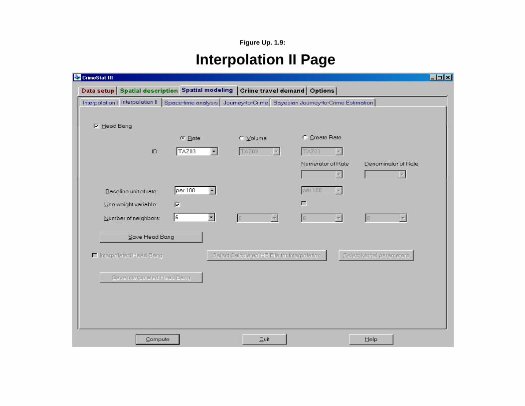
Figure Up. 1.9:

Interpolation II Page

37

to be like its neighbors. In this case, extreme rates, either high or low, are reduced to moderate levels(smoothed) and, thereby, minimize the potential for ‘peak’ or ‘valleys’ as well as maintaining sensitivitywhere there are real edges in the data.

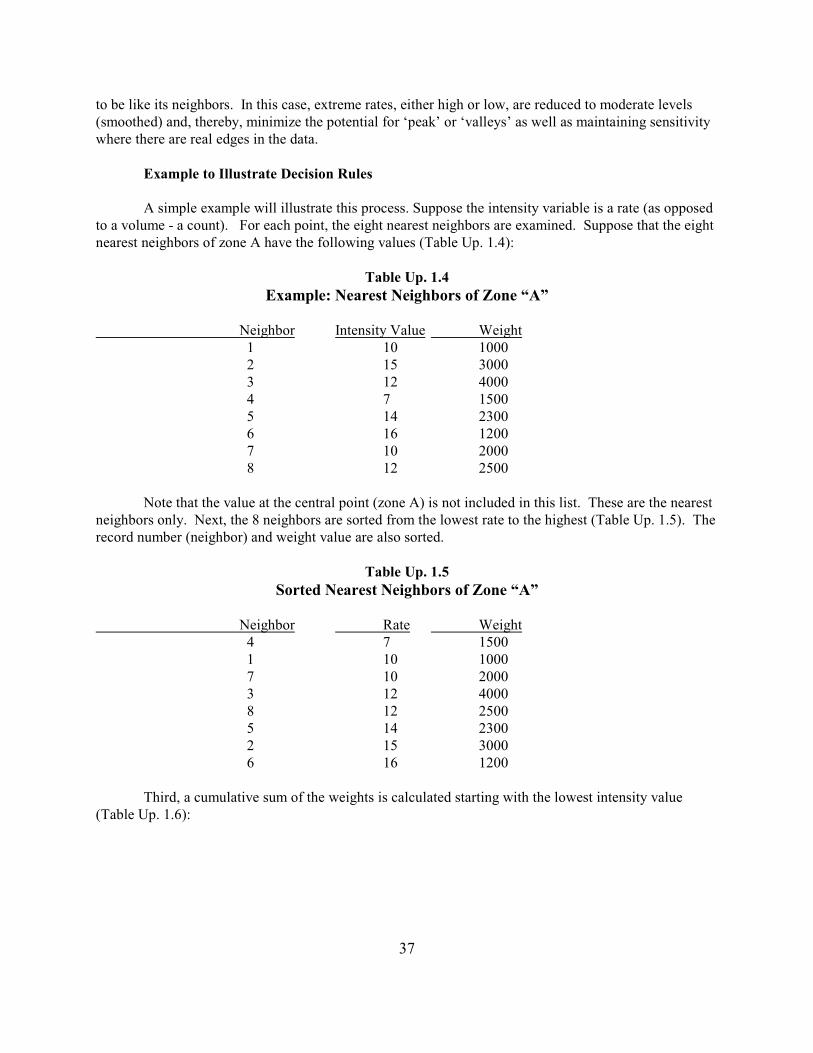
Example to Illustrate Decision Rules

A simple example will illustrate this process. Suppose the intensity variable is a rate (as opposedto a volume - a count). For each point, the eight nearest neighbors are examined. Suppose that the eightnearest neighbors of zone A have the following values (Table Up. 1.4):

Table Up. 1.4

Example: Nearest Neighbors of Zone “A”

Neighbor Intensity Value Weight 1 10 1000 2 15 3000 3 12 4000 4 7 1500 5 14 2300 6 16 1200 7 10 2000 8 12 2500

Note that the value at the central point (zone A) is not included in this list. These are the nearestneighbors only. Next, the 8 neighbors are sorted from the lowest rate to the highest (Table Up. 1.5). Therecord number (neighbor) and weight value are also sorted.

Table Up. 1.5

Sorted Nearest Neighbors of Zone “A”

Neighbor Rate Weight 4 7 1500 1 10 1000 7 10 2000 3 12 4000 8 12 2500 5 14 2300 2 15 3000 6 16 1200

Third, a cumulative sum of the weights is calculated starting with the lowest intensity value(Table Up. 1.6):

38

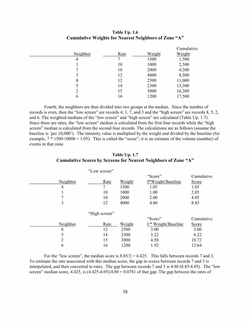
Table Up. 1.6

Cumulative Weights for Nearest Neighbors of Zone “A”

CumulativeNeighbor Rate Weight Weight 4 7 1500 1,500 1 10 1000 2,500 7 10 2000 4,500 3 12 4000 8,500 8 12 2500 11,000 5 14 2300 13,300 2 15 3000 16,300 6 16 1200 17,500

Fourth, the neighbors are then divided into two groups at the median. Since the number ofrecords is even, then the “low screen” are records 4, 1, 7, and 3 and the “high screen” are records 8, 5, 2,and 6. The weighted medians of the “low screen” and “high screen” are calculated (Table Up. 1.7). Since these are rates, the “low screen” median is calculated from the first four records while the “highscreen” median is calculated from the second four records. The calculations are as follows (assume thebaseline is ‘per 10,000’). The intensity value is multiplied by the weight and divided by the baseline (forexample, 7 * 1500/10000 = 1.05). This is called the “score”; it is an estimate of the volume (number) ofevents in that zone.

Table Up. 1.7

Cumulative Scores by Screens for Nearest Neighbors of Zone “A”

“Low screen”“Score” Cumulative

Neighbor Rate Weight I*Weight/Baseline Score 4 7 1500 1.05 1.05 1 10 1000 1.00 2.05 7 10 2000 2.00 4.05 3 12 4000 4.80 8.85

“High screen”“Score” Cumulative

Neighbor Rate Weight I * Weight/Baseline Score 8 12 2500 3.00 3.00 5 14 2300 3.22 6.22 2 15 3000 4.50 10.72 6 16 1200 1.92 12.64

For the “low screen”, the median score is 8.85/2 = 4.425. This falls between records 7 and 3. To estimate the rate associated with this median score, the gap in scores between records 7 and 3 isinterpolated, and then converted to rates. The gap between records 7 and 3 is 4.80 (8.85-4.05). The “lowscreen” median score, 4.425, is (4.425-4.05)/4.80 = 0.0781 of that gap. The gap between the rates of

39

records 7 and 3 is 2 (12-10). Thus, 0.0781 of that gap is 0.1563. This is added to the rate of record 7 toyield a low median rate of 10.1563

For the “high screen”, the median score is 12.64/2 = 6.32. This falls between records 5 and 2. Toestimate the rate associated with this median score, the gap in scores between records 5 and 2 isinterpolated, and then converted to rates. The gap between records 5 and 2 is 4.50 (10.72-6.22). The“low screen” median score, 6.32, is (6.32-6.22)/4.50 = 0.0222 of that gap. The gap between the rates ofrecords 5 and 2 is 1 (15-14). Thus, 0.0222 of that gap is 0.0222. This is added to the rate of record 5 toyield a high median rate of 14.0222.

Finally, the rate associated with the central zone (zone A in our example) is compared to thesetwo medians. If its rate falls between these medians, then it keeps its value. For example, if the rate ofzone A is 13, then that falls between the two medians (10.1563 and 14.0222).

On the other hand, if its rate falls outside this range (either lower than the low median or higherthan the high median), its value is determined by its weight relative to the screen to which it is closest.For example, suppose zone A has a rate of 15 with a weight of 1700. In this case, its rate is higher thanthe high median (14.0222) but its weight is smaller than three of the weights in the high screen. Therefore, it takes the high median as its new smoothed value. Relative to its neighbors, it is smallerthan three of them so that its value is probably too high.

But, suppose it has a rate of 15 and a weight of 3000? Even though its rate is higher than thehigh median, its weight is also higher than the four neighbors making up the high screen. Consequently,it keeps its value. Relative to its neighbors, it is a large zone and its value is probably accurate.

For volumes, the comparison is simpler because all weights are equal. Consequently, the volumeof the central zone is compared directly to the two medians. If it falls between the medians, it keeps itsvalue. If it falls outside the medians, then it takes the median to which it is closest (the high median if ithas a higher value or the low median if it has a lower value).

Setup

For either a rate or a volume, the statistic requires an intensity variable in the primary file. Theuser must specify whether the variable to be smoothed is a rate variable, a volume variable, or twovariables that are to be combined into a rate. If a weight is to be used (for either a rate or the creating ofa rate from two volume variables), it must be defined as a Weight on the Primary File page. Note that ifthe variable is a rate, it probably should be weighted. A typical weighting variable is the population sizeof the zone.

The user has to complete the following steps to run the routine:

1. Define input file and coordinates on the Primary File page

2. Define an intensity variable, Z(intensity), on the Primary File page.

3. OPTIONAL: Define a weighting variable in the weight field on the Primary File page(for rates and for the creating of rates from two volume variables)

40

4. Define an ID variable to identify each zone.

5. Select data type:

A. Rate: the variable to be smoothed is a rate variable which calculates the numberof events (the numerator) relative to a baseline variable (the denominator).

a. The baseline units should be defined, which is an assumed multiplier inpowers of 10. The default is ‘per 100' (percentages) but other choicesare 0 (no multiplier used), ‘per 10' (rate is multiplied by 10), ‘per 1000',‘per 10,000', ‘per 100,000', and ‘per 1,000,000'. This is not used in thecalculation but for reference only.

b. If a weight is to be used, the ‘Use weight variable’ box should bechecked.

B. Volume: the variable to be smoothed is a raw count of the number of events. There is no baseline used.

C. Create Rate: A rate is to be calculated by dividing one variable by another.

a. The user must define the numerator variable and the denominatorvariable.

b. The baseline rate must be defined, which is an assumed multiplier inpowers of 10. The default is ‘per 100' (percentages) but other choicesare 1 (no multiplier used), ‘per 10' (rate is multiplied by 10), ‘per 1000',‘per 10,000', ‘per 100,000', and ‘per 1,000,000'. This is used in thecalculation of the rate.

c. If a weight is to be used, the ‘Use weight variable’ box should bechecked.

6. Select number of neighbors. The number of neighbors can run from 4 through 40. Thedefault is 6. If the number of neighbors selected is even, the routine divides the data setinto two equal-sized groups. If the number of neighbors selected is odd, then the middlezone is used in calculating both the low median and the high median. Itis recommendedthat an even number of neighbors be used (e.g., 4, 6, 8, 10, 12).

7. Select output file. The output can be saved as a dbase ‘dbf’ file. If the output file is arate, then the prefix RateHB is used. If the output is a volume, then the prefix VolHB isused. If the output is a created rate, then the prefix CrateHB is used.

8. Run the routine by clicking ‘Compute’.

41

Output

The Head Bang routine creates a ‘dbf’ file with the following variables:

1. The ID field2. The X coordinate3. The Y coordinate4. The smoothed intensity variable (called ‘Z_MEDIAN’). Note that this is not a Z

score but a smoothed intensity (Z) value5. The weight applied to the smoothed intensity variable. This will be

automatically 1 if no weighting is applied.

The ‘dbf’ file can then be linked to the input ‘dbf’ file by using the ID field as a matchingvariable. This would be done if the user wants to map the smoothed intensity variable.

Example 1: Using the Head Bang Routine for Mapping Houston Burglaries

Earlier, Figure Up. 1.1 showed a map of Houston burglaries by traffic analysis zones; the mappedvariable is the number of burglaries committed in 2006. On the Head Bang interface, the ‘Volume’ boxis checked, indicating that the number of burglaries will be estimated. The number of neighbors is left atthe default 6. The output ‘dbf’ file was then linked to the input ‘dbf’ file using the ID field to allow thesmoothed intensity values to be mapped.

Figure Up. 1.10 shows a smoothed map of the number of burglaries conducted by the Head Bangroutine. With both maps, the number of intervals that are mapped is 5. Comparing this map with FigureUp. 1.1, it can be seen that there are fewer zones in the lowest interval/bin (in yellow). The actual countsare 528 zones with scores of less than 10 in Figure Up. 1.1 compared to 498 zones in Figure Up. 1.10. Also, there are fewer zones in the highest interval/bin (in black) as well. The actual counts are 215 zoneswith scores of 40 or more in Figure Up. 1.1 compared to 181 zones in Figure Up 1.

In other words, the Head Bang routine has eliminated many of the highest values by assigningthem to the median values of their neighbors, either those of the ‘high screen’ or the ‘low screen’.

Example 2: Using the Head Bang Routine for Mapping Burglary Rates

The second example shows how the Head Bang routine can smooth rates. In the Houstonburglary data base, a rate variable was created which divided the number of burglaries in 2006 by thenumber of households in 2006. This variable was then multiplied by 1000 to minimize the effects ofdecimal place (the baseline unit). Figure Up. 1.11 shows the raw burglary rate (burglaries per 1,000households) for the City of Houston in 2006.

The Head Bang routine was set up to estimate a rate for this variable (Burglaries Per 1000Households). On the Primary File page, the intensity variable was defined as the calculated rate(burglaries per 1,000 households) because the Head Bang will smooth the rate. Also, a weight variable isselected on the Primary File page. In this example, the weight variable was the number of households.

Figure Up. 1.10:

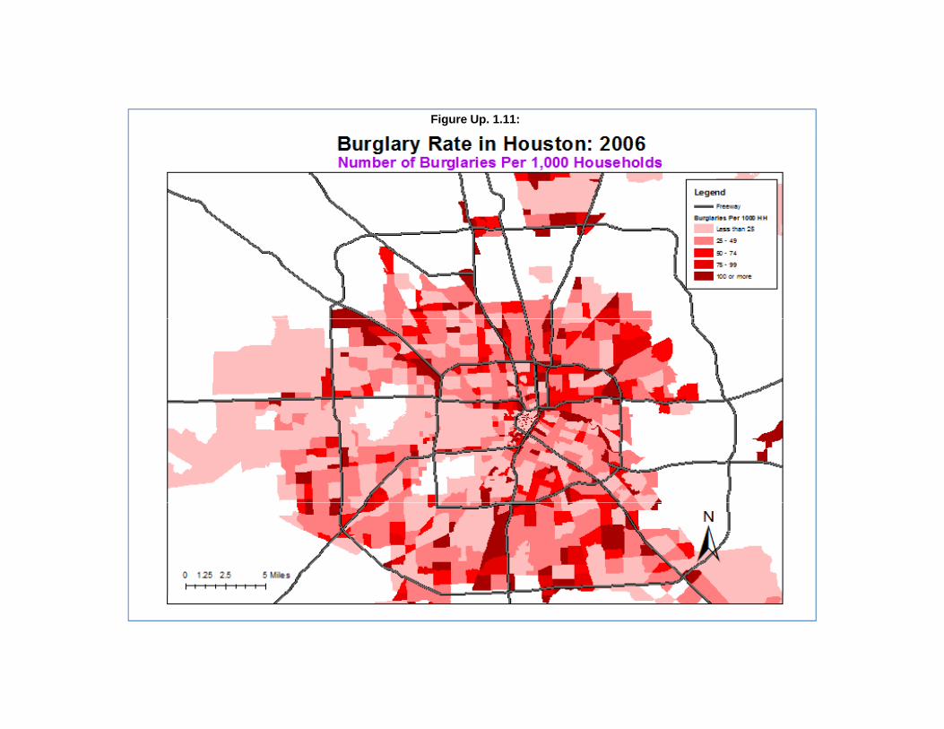
Figure Up. 1.11:

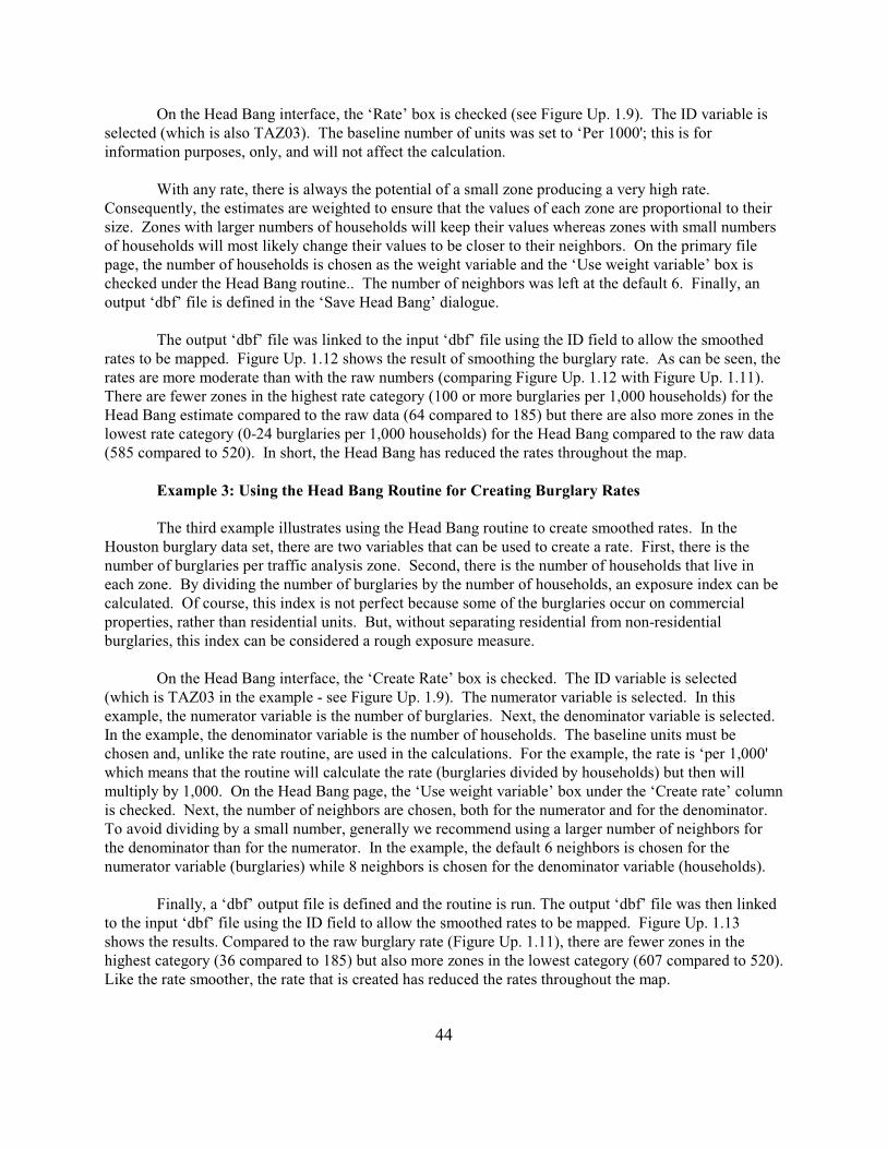
44

On the Head Bang interface, the ‘Rate’ box is checked (see Figure Up. 1.9). The ID variable isselected (which is also TAZ03). The baseline number of units was set to ‘Per 1000'; this is forinformation purposes, only, and will not affect the calculation.

With any rate, there is always the potential of a small zone producing a very high rate. Consequently, the estimates are weighted to ensure that the values of each zone are proportional to theirsize. Zones with larger numbers of households will keep their values whereas zones with small numbersof households will most likely change their values to be closer to their neighbors. On the primary filepage, the number of households is chosen as the weight variable and the ‘Use weight variable’ box ischecked under the Head Bang routine.. The number of neighbors was left at the default 6. Finally, anoutput ‘dbf’ file is defined in the ‘Save Head Bang’ dialogue.

The output ‘dbf’ file was linked to the input ‘dbf’ file using the ID field to allow the smoothedrates to be mapped. Figure Up. 1.12 shows the result of smoothing the burglary rate. As can be seen, therates are more moderate than with the raw numbers (comparing Figure Up. 1.12 with Figure Up. 1.11). There are fewer zones in the highest rate category (100 or more burglaries per 1,000 households) for theHead Bang estimate compared to the raw data (64 compared to 185) but there are also more zones in thelowest rate category (0-24 burglaries per 1,000 households) for the Head Bang compared to the raw data(585 compared to 520). In short, the Head Bang has reduced the rates throughout the map.

Example 3: Using the Head Bang Routine for Creating Burglary Rates

The third example illustrates using the Head Bang routine to create smoothed rates. In theHouston burglary data set, there are two variables that can be used to create a rate. First, there is thenumber of burglaries per traffic analysis zone. Second, there is the number of households that live ineach zone. By dividing the number of burglaries by the number of households, an exposure index can becalculated. Of course, this index is not perfect because some of the burglaries occur on commercialproperties, rather than residential units. But, without separating residential from non-residentialburglaries, this index can be considered a rough exposure measure.

On the Head Bang interface, the ‘Create Rate’ box is checked. The ID variable is selected(which is TAZ03 in the example - see Figure Up. 1.9). The numerator variable is selected. In thisexample, the numerator variable is the number of burglaries. Next, the denominator variable is selected. In the example, the denominator variable is the number of households. The baseline units must bechosen and, unlike the rate routine, are used in the calculations. For the example, the rate is ‘per 1,000'which means that the routine will calculate the rate (burglaries divided by households) but then willmultiply by 1,000. On the Head Bang page, the ‘Use weight variable’ box under the ‘Create rate’ columnis checked. Next, the number of neighbors are chosen, both for the numerator and for the denominator. To avoid dividing by a small number, generally we recommend using a larger number of neighbors forthe denominator than for the numerator. In the example, the default 6 neighbors is chosen for thenumerator variable (burglaries) while 8 neighbors is chosen for the denominator variable (households).

Finally, a ‘dbf’ output file is defined and the routine is run. The output ‘dbf’ file was then linkedto the input ‘dbf’ file using the ID field to allow the smoothed rates to be mapped. Figure Up. 1.13shows the results. Compared to the raw burglary rate (Figure Up. 1.11), there are fewer zones in thehighest category (36 compared to 185) but also more zones in the lowest category (607 compared to 520). Like the rate smoother, the rate that is created has reduced the rates throughout the map.

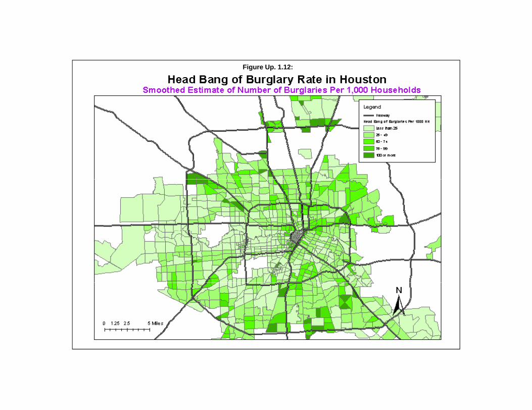
Figure Up. 1.12:

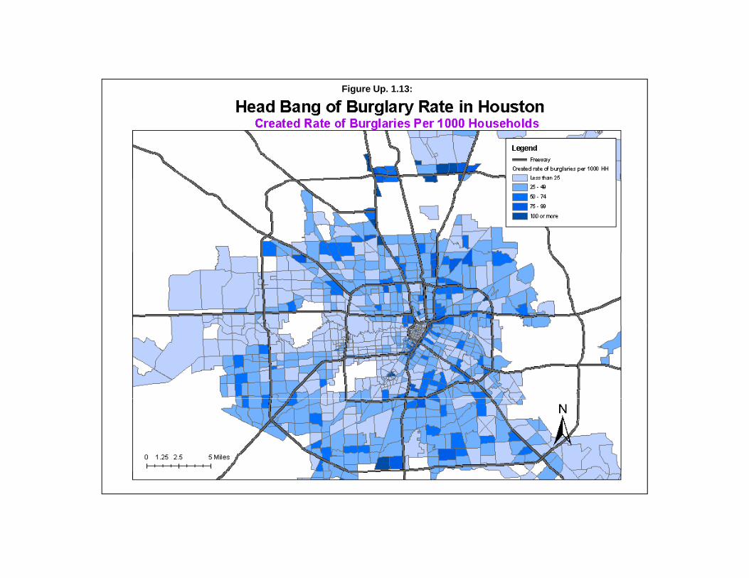
Figure Up. 1.13:

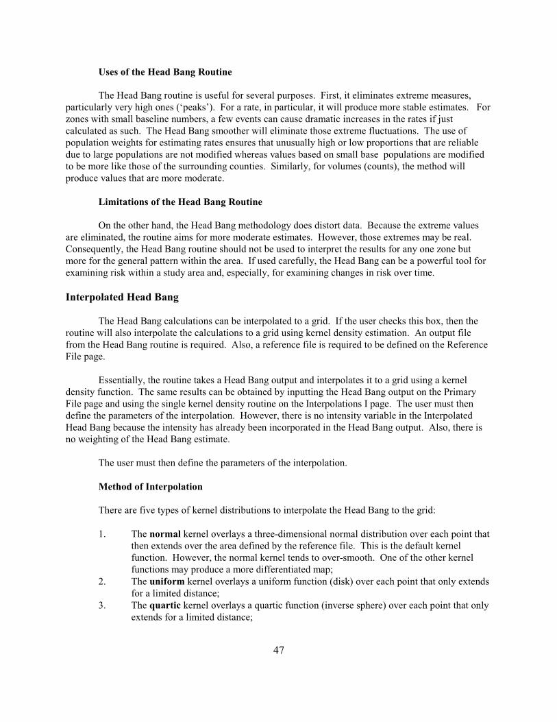
47

Uses of the Head Bang Routine

The Head Bang routine is useful for several purposes. First, it eliminates extreme measures,particularly very high ones (‘peaks’). For a rate, in particular, it will produce more stable estimates. Forzones with small baseline numbers, a few events can cause dramatic increases in the rates if justcalculated as such. The Head Bang smoother will eliminate those extreme fluctuations. The use ofpopulation weights for estimating rates ensures that unusually high or low proportions that are reliabledue to large populations are not modified whereas values based on small base populations are modifiedto be more like those of the surrounding counties. Similarly, for volumes (counts), the method willproduce values that are more moderate.

Limitations of the Head Bang Routine

On the other hand, the Head Bang methodology does distort data. Because the extreme valuesare eliminated, the routine aims for more moderate estimates. However, those extremes may be real.Consequently, the Head Bang routine should not be used to interpret the results for any one zone butmore for the general pattern within the area. If used carefully, the Head Bang can be a powerful tool forexamining risk within a study area and, especially, for examining changes in risk over time.

Interpolated Head Bang

The Head Bang calculations can be interpolated to a grid. If the user checks this box, then theroutine will also interpolate the calculations to a grid using kernel density estimation. An output filefrom the Head Bang routine is required. Also, a reference file is required to be defined on the ReferenceFile page.

Essentially, the routine takes a Head Bang output and interpolates it to a grid using a kerneldensity function. The same results can be obtained by inputting the Head Bang output on the PrimaryFile page and using the single kernel density routine on the Interpolations I page. The user must thendefine the parameters of the interpolation. However, there is no intensity variable in the InterpolatedHead Bang because the intensity has already been incorporated in the Head Bang output. Also, there isno weighting of the Head Bang estimate.

The user must then define the parameters of the interpolation.

Method of Interpolation

There are five types of kernel distributions to interpolate the Head Bang to the grid:

1. The normal kernel overlays a three-dimensional normal distribution over each point thatthen extends over the area defined by the reference file. This is the default kernelfunction. However, the normal kernel tends to over-smooth. One of the other kernelfunctions may produce a more differentiated map;

2. The uniform kernel overlays a uniform function (disk) over each point that only extendsfor a limited distance;

3. The quartic kernel overlays a quartic function (inverse sphere) over each point that onlyextends for a limited distance;

48

4. The triangular kernel overlays a three-dimensional triangle (cone) over each point thatonly extends for a limited distance; and

5. The negative exponential kernel overlays a three dimensional negative exponentialfunction over each point that only extends for a limited distance.

The different kernel functions produce similar results though the normal is generally smootherfor any given bandwidth.

Choice of Bandwidth

The kernels are applied to a limited search distance, called 'bandwidth'. For the normal kernel,bandwidth is the standard deviation of the normal distribution. For the uniform, quartic, triangular andnegative exponential kernels, bandwidth is the radius of a circle defined by the surface. For all types,larger bandwidth will produce smoother density estimates and both adaptive and fixed bandwidthintervals can be selected.

Adaptive bandwidth

An adaptive bandwidth distance is identified by the minimum number of other points foundwithin a circle drawn around a single point. A circle is placed around each point, in turn, and the radiusis increased until the minimum sample size is reached. Thus, each point has a different bandwidthinterval. The user can modify the minimum sample size. The default is 100 points. If there is a smallsample size (e.g., less than 500), then a smaller minimum sample size would be more appropriate).

Fixed bandwidth

A fixed bandwidth distance is a fixed interval for each point. The user must define the intervaland the distance units by which it is calculated (miles, nautical miles, feet, kilometers, meters.)

Output (areal) units

Specify the areal density units as points per square mile, per squared nautical miles, per squarefeet, per square kilometers, or per square meters. The default is points per square mile.

Calculate Densities or Probabilities

The density estimate for each cell can be calculated in one of three ways:

Absolute densities

This is the number of points per grid cell and is scaled so that the sum of all grid cells equals thesample size. This is the default.

Relative densities

For each grid cell, this is the absolute density divided by the grid cell area and is expressed in theoutput units (e.g., points per square mile)

49

Probabilities

This is the proportion of all incidents that occur in each grid cell. The sum of all grid cellsequals 1.

Select whether absolute densities, relative densities, or probabilities are to be output for eachcell. The default is absolute densities.

Output

The results can be output as a Surfer for Windows file (for both an external or generatedreference file) or as an ArcView '.shp', MapInfo '.mif', Atlas*GIS '.bna', ArcView Spatial Analyst 'asc', orASCII grid 'grd' file (only if the reference file is generated by CrimeStat.) The output file is saved asIHB<root name> with the root name being provided by the user.

Example: Using the Interpolated Head Bang to Visualize Houston Burglaries

The Houston burglary data set was, first, smoothed using the Head Bang routine (Figure Up. 1.10above) and, second, interpolated to a grid using the Interpolated Head Bang routine. The kernel chosenwas the default normal distribution but with a fixed bandwidth of 1 mile. Figure Up. 1.14 shows theresults of the interpolation.

To compare this to an interpolation of the original data, the raw number of burglaries in eachzone were interpolated using the single kernel density routine. The kernel used was also the normaldistribution with a fixed bandwidth of 1 mile. Figure Up. 1.15 shows the results of interpolating the rawburglary numbers.

An inspection of these two figures show that they both capture the areas with the highestburglary density. However, the Interpolated Head Bang produces fewer high density cells which, in turn,allows the moderately high cells to stand out. For example, in southwest Houston, the Interpolated HeadBang shows two small areas of moderately high density of burglaries whereas the raw interpolationmerges these together.

Advantages and Disadvantages of the Interpolated Head Bang

The Interpolated Head Bang routine has the same advantages and disadvantages as the HeadBang routine. Its advantages are that it captures the strongest tendencies by eliminating ‘peaks’ and‘valleys’. But, it also does this by distorting the data. The user has to determine whether the eliminationof areas with very high or very low density values are real just due to small number of events.

For law enforcement applications, this may or may not be an advantage. Some hot spots, forexample, are small areas where there are a many crime events. Smoothing the data may eliminate thevisibility of these. On the other hand, large hot spots will generally survive the smoothing processbecause the number of events is large and will usually spread to adjacent grid cells. As usual, the userhas to be aware of the advantages and disadvantages in order to decide whether a particular tool, such asthe interpolated Head Bang is useful or not.

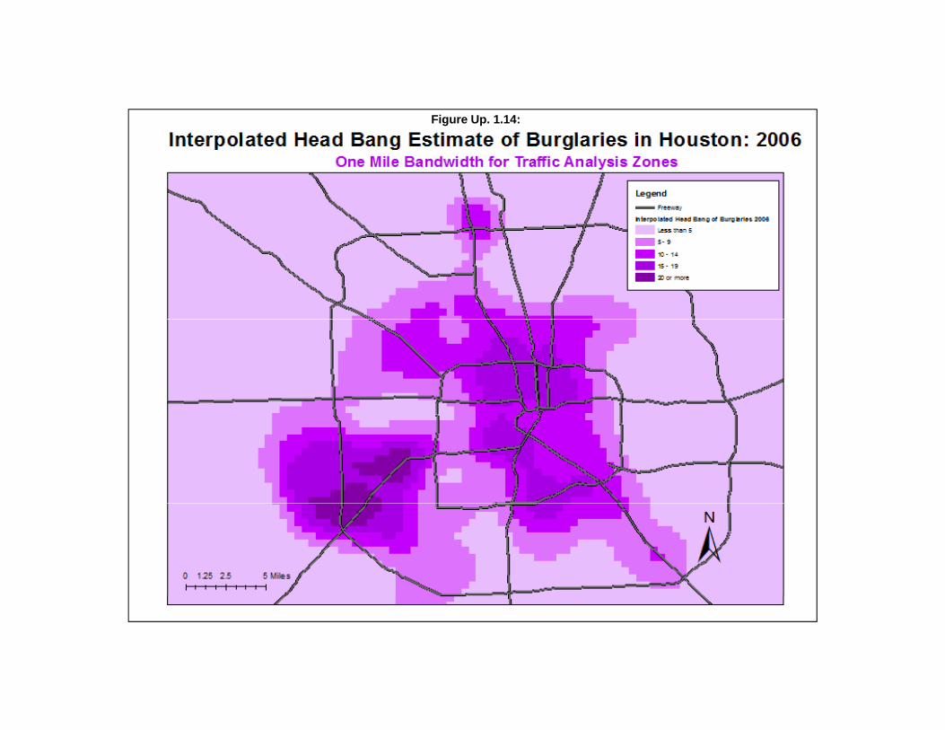
Figure Up. 1.14:

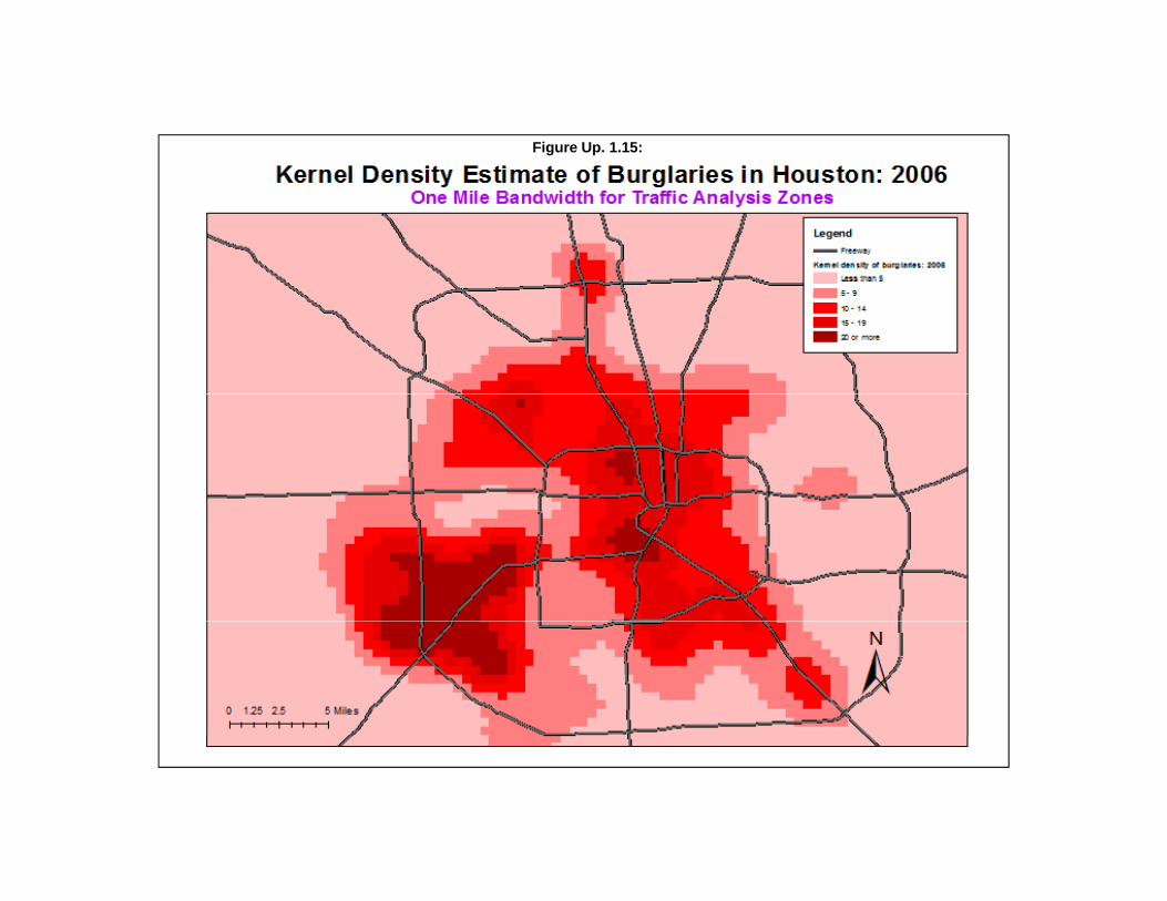
Figure Up. 1.15:

52

Bayesian Journey to Crime Module

The Bayesian Journey to Crime module (Bayesian Jtc) are a set of tools for estimating the likelyresidence location of a serial offender. It is an extension of the distance-based Journey to crime routine(Jtc) which uses a typical travel distance function to make guesses about the likely residence location. The extension involves the use an origin-destination matrix which provides information about theparticular origins of offenders who committed crimes in particular destinations.

First, the theory behind the Bayesian Jtc routine will be described. Then, the data requirementswill be discussed. Finally, the routine will be illustrated with some data from Baltimore County.

Bayesian Probability

Bayes Theorem is a formulation that relates the conditional and marginal probabilitydistributions of random variables. The marginal probability distribution is a probability independent ofany other conditions. Hence, P(A) and P(B) is the marginal probability (or just plain probability) of Aand B respectively.

The conditional probability is the probability of an event given that some other event hasoccurred. It is written in the form of P(A|B) (i.e., event A given that event B has occurred). In probabilitytheory, it is defined as:

P (A and B)P(A|B) = ----------------- (Up. 1.32)

P(B)

Conditional probabilities can be best be seen in contingency tables. Table Up. 1.8 below show apossible sequence of counts for two variables (e.g., taking a sample of persons and counting their gender- male = 1; female = 0, and their age - older than 30 = 1; 30 or younger = 0). The probabilities can beobtained just by counting:

P(A) = 30/50 = 0.6P(B) = 35/50 = 0.7P(A and B) = 25/50 = 0.5P(A or B) = (30+35-25)/50 = 0.8P(A|B) = 25/35 = 0.71P(B|A) = 25/30 = 0.83

53

Table Up. 1.8:

Example of Determining Probabilities by Counting

A has A hasNOT Occurred Occurred TOTAL

B has NOTOccurred 10 5 15

B hasOccurred 10 25 35

TOTAL 20 30 50

However, if four of these six calculations are known, Bayes Theorem can be used to solve for theother two. Two logical terms in probability are the ‘and’ and ‘or’ conditions. Usually, the symbol c isused for ‘or’ and 1 is used for ‘and’, but writing it in words makes it easier to understand. The followingtwo theorems define these.

1. The probability that either A or B will occur is

P(A or B) = P(A) + P(B) - P(A and B) (Up. 1.33)

2. The probability that both A and B will occur is:

P(A and B) = P(A) * P(B|A) = P(B)*P(A|B) (Up. 1.34)

Bayes Theorem relates the two equivalents of the ‘and’ condition together.

P(B) * P(A|B) = P(A) * P(B|A) (Up. 1.35)

P(A) * P(B|A)P(A|B) = ------------------- (Up. 1.36)

P(B)

The theorem is sometimes called the ‘inverse probability’ in that it can invert two conditionalprobabilities:

P(B) * P(A|B)P(B|A) = -------------------- (Up. 1.37)

P(A)

By plugging in the values from the example in Table Up. 1.8, the reader can verify that BayesTheorem produces the correct results (e.g., P(B|A) = 0.7 * 0.71/0.6 = 0.83).

54

Bayesian Inference

In the statistical interpretation of Bayes Theorem, the probabilities are estimates of a randomvariable. Let è be a parameter of interest and let X be some data. Thus, Bayes Theorem can beexpressed as:

P(X|è) * P(è)P(è|X) = ------------------- (Up. 1.38)

P(X)

Interpreting this equation, P(è|X) is the probability of è given the data, X. P(è) is the probabilitythat è has a certain distribution and is often called the prior probability. P(X|è) is the probability that thedata would be obtained given that è is true and is often called the likelihood function (i.e., it is thelikelihood that the data will be obtained given the distribution of è). Finally, P(X) is the marginalprobability of the data, the probability of obtaining the data under all possible scenarios; essentially, it isthe data.

The equation can be rephrased in logical terms:

Posterior Likelihood of Priorprobability that obtaining the data probabilityè is true given the given è is true * of èdata, X = --------------------------------------------------------- (Up. 1.39)

Marginal probability of X

In other words, this formulation allows an estimate of the probability of a particular parameter, è,to be updated given new information. Since è is the prior probability of an event, given some new data,X, Bayes Theorem can be used to update the estimate of è. The prior probability of è can come fromprior studies, an assumption of no difference between any of the conditions affecting è, or an assumedmathematical distribution. The likelihood function can also come from empirical studies or an assumedmathematical function. Irrespective of how these are interpreted, the result is an estimate of theparameter, è, given the evidence, X. This is called the posterior probability (or posterior distribution).

A point that is often made is that the prior probability of obtaining the data (the denominator ofthe above equation) is not known or can’t easily be evaluated. The data are what was obtained fromsome data gathering exercise (either experimental or from observations). Thus, it is not easy to estimateit. Consequently, often the numerator only is used for estimate the posterior probability since

P(è|X) % P(X|è) * P(è) (Up. 1.40)

where % means ‘proportional to’. In some statistical methods (e.g., the Markov Chain Monte Carlosimulation, or MCMC), the parameter of interest is estimated by thousands of random simulations usingapproximations to P(X|è) and P(è) respectively.

The key point behind this logic is that an estimate of a parameter can be updated by additionalnew information systematically. The formula requires that a prior probability value for the estimate begiven with new information being added which is conditional on the prior estimate, meaning that it

55

factors in information from the prior. Bayesian approaches are increasingly be used provide estimatesfor complex calculations that previously were intractable (Denison, Holmes, Mallilck, and Smith, 2002;Lee, 2004; Gelman, Carlin, Stern, and Rubin, 2004).

Application of Bayesian Inference to Journey to Crime Analysis

Bayes Theorem can be applied to the journey to crime methodology. In the Journey to Crime(Jtc) method, an estimate is made about where a serial offender is living. The Jtc method produces aprobability estimate based on an assumed travel distance function (or, in more refined uses of themethod, travel time). That is, it is assumed that an offender follows a typical travel distance function. This function can be estimated from prior studies (Canter and Gregory, 1994; Canter, 2003) or fromcreating a sample of known offenders - a calibration sample (Levine, 2004) or from assuming that everyoffender follows a particular mathematical function (Rossmo, 1995; 2000). Essentially, it is a priorprobability for a particular location, P(è). That is, it is a guess about where the offender lives on theassumption that the offender of interest is following an existing travel distance model.

However, additional information from a sample of known offenders where both the crimelocation and the residence location are known can be added. This information would be obtained fromarrest records, each of which will have a crime location defined (a ‘destination’) and a residence location(an ‘origin’). If these locations are then assigned to a set of zones, a matrix that relates the origin zonesto the destination zones can be created (Figure Up. 1.16). This is called an origin-destination matrix (ora trip distribution matrix or an O-D matrix, for short).

In this figure, the numbers indicate crimes that were committed in each destination zone thatoriginated (i.e., the offender lived) in each origin zone. For example, taking the first row in figure Up.1.16, there were 37 crimes that were committed in zone 1 and in which the offender also lived in zone 1;there were 15 crimes committed in zone 2 in which the offender lived in zone 1; however, there wereonly 7 crimes committed in zone 1 in which the offender lived in zone 2; and so forth.

Note two things about the matrix. First, the number of origin zones can be (and usually is)greater than the number of destination zones because crimes can originate outside the study area. Second, the marginal totals have to be equal. That is, the number of crimes committed in all destinationzones has to equal the number of crimes originating in all origin zones.

This information can be treated as the likelihood estimate for the Journey to Crime framework. That is, if a certain distribution of incidents committed by a particular serial offender is known, then thismatrix can be used to estimate the likely origin zones from which offenders came, independent of anyassumption about travel distance. In other words, this matrix is equivalent to the likelihood function inequation Up. 1.38, which is repeated below:

P(X|è) * P(è)P(è|X) = ----------------- repeat (Up. 1.38)

P(X)

Thus, the estimate of the likely location of a serial offender can be improved by updating theestimate from the Jtc method, P(è), with information from an empirically-derived likelihood estimate,P(X|è). Figure Up. 1.17 illustrates how this process works. Suppose one serial offender committed

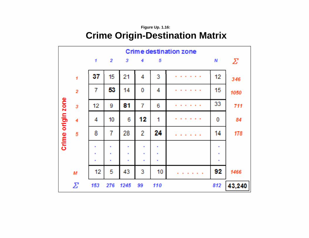
Crime Origin-Destination MatrixFigure Up. 1.16:

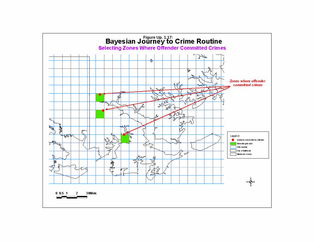
Figure Up. 1.17:

58

crimes in three zones. These are shown in terms of grid cell zones. In reality, most zones are not gridcell shaped but are irregular. However, illustrating it with grid cells makes it more understandable. Using an O-D matrix based on those cells, only the destination zones corresponding to those cells areselected (Figure Up. 1.18). This process is repeated for all serial offenders in the calibration file whichresults in marginal totals that correspond to frequencies for those serial offenders who committed crimesin the selected zones. In other words, the distribution of crimes is conditioned on the locations thatcorrespond to where the serial offender of interest committed his or her crimes. It is a conditionalprobability.

But, what about the denominator, P(X)? Essentially, it is the spatial distribution of all crimesirrespective of which particular model or scenario we’re exploring. In practice, it is very difficult, if notimpossible, to estimate the probability of obtaining the data under all circumstances.

I’m going to change the symbols at this point so the Jtc represents the distance-based Journey toCrime estimate, O represents an estimate based on an origin-destination matrix, and O|Jtc represents theparticular origins associated with crimes committed in the same zones as that identified in the Jtcestimate. Therefore, there are three different probability estimates of where an offender lives:

1. A probability estimate of the residence location of a single offender based on thelocation of the incidents that this person committed and an assumed travel distancefunction, P(Jtc);

2. A probability estimate of the residence location of a single offender based on a generaldistribution of all offenders, irrespective of any particular destinations for incidents,P(O). Essentially, this is the distribution of origins irrespective of the destinations; and

3. A probability estimate of the residence location of a single offender based on thedistribution of offenders given the distribution of incidents committed by otheroffenders who committed crimes in the same locaiton, P(O|Jtc).

Therefore, Bayes Theorem can be used to create an estimate that combines information bothfrom a travel distance function and an origin-destination matrix (equation Up. 1.38):

P(Jtc|O) % P(O|Jtc) * P(Jtc) (Up. 1.41)

in which the posterior probability of the journey to crime location conditional on the origin-destinationmatrix is proportional to the product of the prior probability of the journey to crime function, P(Jtc), andthe conditional probability of the origins for other offenders who committed crimes in the same locations.This will be called the product probability. As mentioned above, it is very difficult, if not impossible, todetermine the probability of obtaining the data under any circumstance. Consequently, the Bayesianestimate is usually calculated only with respect to the numerator, the product of the prior probability andthe likelihood function.

A very rough approximation to the full Bayesian probability can be obtained by taking theproduct probability and dividing it by the general probability: It related the the product term (thenumerator) to the general distribution of crimes. This will produce a relative risk measure, which iscalled Bayesian risk.

Crime destination zone

Conditional Origin-Destination MatrixDestination zones where serial

ff d itt d iMarginal totals for

Figure Up. 1.18:

1 2 3 4 5 N

Crime destination zone

G

offender committed crimesg

selected zones only

1

2

. . . . . .

. . . . . .53 0

15 4 12

15

121

205

3

4

. . . . . .

. . . . . .gin

zone

12 0 35

9

10

7 33 65

5

. . .

. . . . . .

Crim

e or

i

407 2 14

M

.

...

.

.

92 1415 3M . . . . . . 92

G

1415 3

99276 812 1,597

60

P(O|Jtc) * P(Jtc)P(Jtc|O) = ------------------------ (Up. 1.42)

P(O)

In this case, the product probability is being compared to the general distribution of the origins of alloffenders irrespective of where they committed their crimes. Note that this measure will correlate withthe product term because they both have the same numerator.

The Bayesian Journey to Crime Estimation Module

The Bayesian Journey to Crime estimation module is made up of two routines, one fordiagnosing which Journey to Crime method is best and one for applying that method to a particular serialoffender. Figure Up. 1.19 shows the layout of the module.

Data Preparation for Bayesian Journey to Crime Estimation

There are four data sets that are required:

1. The incidents committed by a single offender for which an estimate will be made ofwhere that individual lives;

2. A Journey to Crime travel distance function that estimates the likelihood of an offendercommitting crimes at a certain distance (or travel time if a network is used);

3. An origin-destination matrix; and

4. A diagnostics file of multiple known serial offenders for which both their residence andcrime locations are known.

Serial offender data

For each serial offender for whom an estimate will be made of where that person lives, the dataset should include the location of the incidents committed by the offender. The data are set up as a seriesof records in which each record represents a single event. On each data set, there are X and Ycoordinates identifying the location of the incidents this person has committed (Table Up. 1.9).

Figure Up. 1.19:

Bayesian Journey to Crime Page

62

Table Up. 1.9:

Minimum Information Required for Serial Offenders:Example for Offender Who Committed Seven Incidents

ID UCR INCIDX INCIDYTS7C 430.00 -76.494300 39.2846TS7C 440.00 -76.450900 39.3185TS7C 630.00 -76.460600 39.3157TS7C 430.00 -76.450700 39.3181TS7C 311.00 -76.449700 39.3162TS7C 440.00 -76.450300 39.3178TS7C 341.00 -76.448200 39.3123

Journey to Crime travel function

The Journey to Crime travel function (Jtc) is an estimate of the likelihood of an offendertraveling a certain distance. Typically, it represents a frequency distribution of distances traveled, thoughit could be a frequency distribution of travel times if a network was used to calibrate the function withthe Journey to crime estimation routine. It can come from an a priori assumption about travel distances,prior research, or a calibration data set of offenders who have already been caught. The “CalibrateJourney to Crime function” routine (on the Journey to Crime page under Spatial modeling) can be used toestimate this function. Details are found in chapter 10 of the CrimeStat manual.

The BJtc routine can use two different travel distance functions: 1) An already-calibrateddistance function; and 2) A mathematical formula. Either direct or indirect (Manhattan) distances can beused though the default is direct (see Measurement parameters). In practice, an empirically-derivedtravel function is often as accurate, if not better, than a mathematically-defined one. Given that anorigin-destination matrix is also needed, it is easy for the user to estimate the travel function using the“Calibrate Journey to crime function”.

Origin-destination matrix

The origin-destination matrix relates the number of offenders who commit crimes in one of Nzones who live (originate) in one of M zones, similar to Figure Up. 1.16 above. It can be created fromthe “Calculate observed origin-destination trips” routine (on the ‘Describe origin-destination trips’ pageunder the Trip distribution module of the Crime Travel Demand model).

How many incidents are needed where the origin and destination location are known? Whilethere is no simple answer to this, the numbers ideally should be in the tens of thousands. If there are Ndestinations and M rows, ideally one would want an average of 30 cases for each cell to produce areliable estimate. Obviously, that’s a huge amount of data and one not easily found with any realdatabase. For example, if there are 325 destination zones and 532 origin zones (the Baltimore Countyexample given below), that would be 172,900 individual cells. If the 30 cases or more rule is applied,then that would require 5,187,000 records or more to produce a barely reliable estimate for most cells.

63

The task becomes even more daunting when it is realized that many of these links (cells) havefew or no cases in them as offenders typically travel along certain pathways. Obviously, such a demandfor data is impractical even in the largest jurisdictions. Therefore, we recommend that as much data aspossible be used to produce the origin-destination (O-D) matrix, at least several years worth. The matrixcan be built with what data is available and then periodically updated to produce better estimates.

Diagnostics file for Bayesian Jtc routine

The fourth data set is used for estimating which of several parameters is best at predicting theresidence location of serial offenders in a particular jurisdiction. Essentially, it is a set of serial offenders,each record of which has information on the X and Y coordinates of the residence location as well as thecrime location. For example, offender T7B committed seven incidents while offender S8A committedeight incidents. The records of both offenders are placed in the same file along with the records for allother offenders in the diagnostics file.

The diagnostics file provides information about which of several parameters (to be describedbelow) are best at guessing where an offender lives. The assumption is that if a particular parameter wasbest with the K offenders in a diagnostics file in which the residence location was known, then the sameparameter will also be best for a serial offender for whom the residence location is not known.

How many serial offenders are needed to make up a diagnostics file? Again, there is no simpleanswer to this though the number are much less than for the O-D matrix. Clearly, the more, the bettersince the aim is to identify which parameter is most sensitive with a certain level of precision andaccuracy. I used 88 offenders in my diagnostics file (see below). Certainly, a minimum of 10 would benecessary. But, more would certainly be more accurate. Further, the offender records used in thediagnostics file should be similar in other dimensions to the offender that is being tracked. However, thismay be impractical. In the example data set, I combined offenders who committed different types ofcrimes. The results may be different if offenders who had committed only one type of crimes were tested.

Once the data sets have been collected, they need to be placed in an appended file, with oneserial offender on top of another. Each record has to represent a single incident. Further, the recordshave to be arranged sequentially with all the records for a single offender being grouped together. Theroutine automatically sorts the data by the offender ID. But, to be sure that the result is consistent, thedata should be prepared in this way.

The structure of the records is similar to the example in Table Up. 1.10 below. At the minimum,there is a need for an ID field, and the X and Y coordinates of both crime location and the residencelocation. Thus, in the example, all the records for the first offender (Num 1) are together; all the recordsfor the second offender (Num 2) are together; and so forth. The ID field is any string variable. In TableUp. 1.10, the ID field is labeled “ID”, but any label would be acceptable as long as it is consistent (i.e.,all the records of a single offender are together).

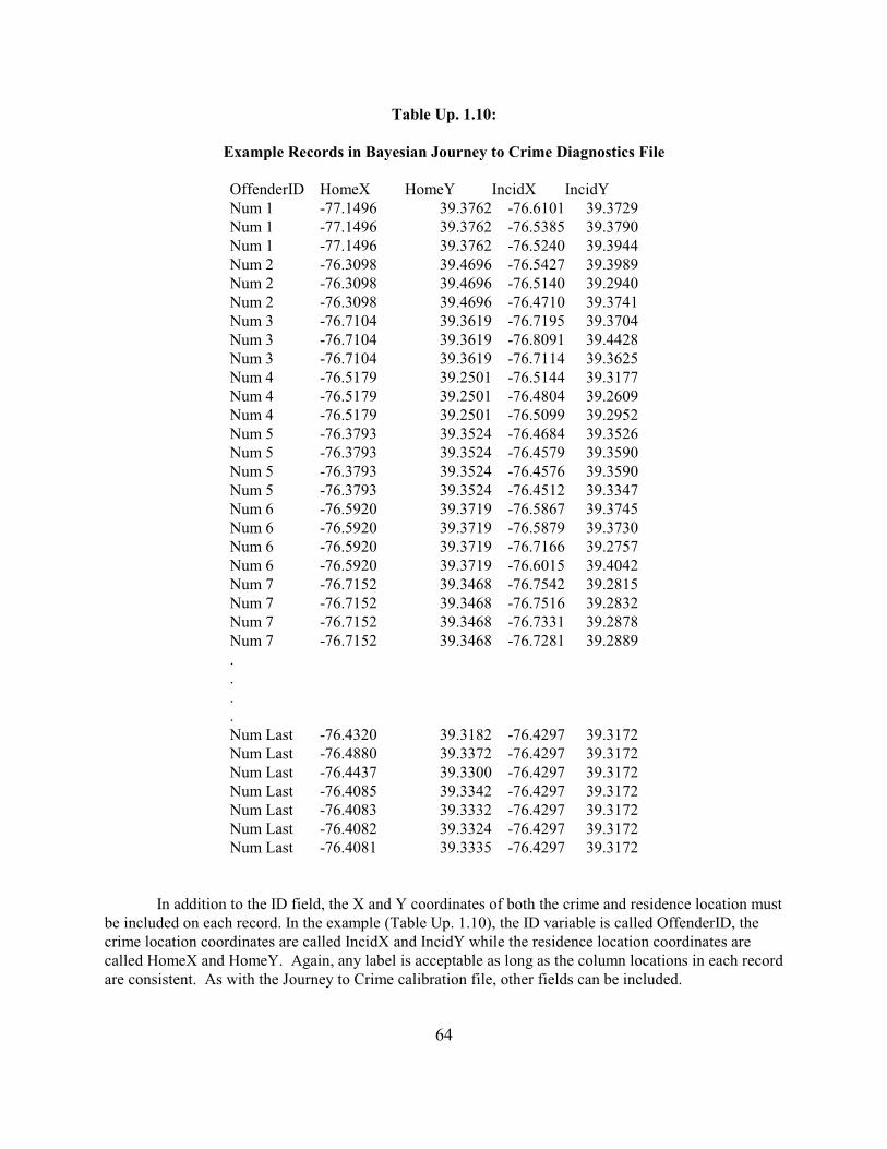
64

Table Up. 1.10:

Example Records in Bayesian Journey to Crime Diagnostics File

OffenderID HomeX HomeY IncidX IncidYNum 1 -77.1496 39.3762 -76.6101 39.3729Num 1 -77.1496 39.3762 -76.5385 39.3790Num 1 -77.1496 39.3762 -76.5240 39.3944Num 2 -76.3098 39.4696 -76.5427 39.3989Num 2 -76.3098 39.4696 -76.5140 39.2940Num 2 -76.3098 39.4696 -76.4710 39.3741Num 3 -76.7104 39.3619 -76.7195 39.3704Num 3 -76.7104 39.3619 -76.8091 39.4428Num 3 -76.7104 39.3619 -76.7114 39.3625Num 4 -76.5179 39.2501 -76.5144 39.3177Num 4 -76.5179 39.2501 -76.4804 39.2609Num 4 -76.5179 39.2501 -76.5099 39.2952Num 5 -76.3793 39.3524 -76.4684 39.3526Num 5 -76.3793 39.3524 -76.4579 39.3590Num 5 -76.3793 39.3524 -76.4576 39.3590Num 5 -76.3793 39.3524 -76.4512 39.3347Num 6 -76.5920 39.3719 -76.5867 39.3745Num 6 -76.5920 39.3719 -76.5879 39.3730Num 6 -76.5920 39.3719 -76.7166 39.2757Num 6 -76.5920 39.3719 -76.6015 39.4042Num 7 -76.7152 39.3468 -76.7542 39.2815Num 7 -76.7152 39.3468 -76.7516 39.2832Num 7 -76.7152 39.3468 -76.7331 39.2878Num 7 -76.7152 39.3468 -76.7281 39.2889....Num Last -76.4320 39.3182 -76.4297 39.3172Num Last -76.4880 39.3372 -76.4297 39.3172Num Last -76.4437 39.3300 -76.4297 39.3172Num Last -76.4085 39.3342 -76.4297 39.3172Num Last -76.4083 39.3332 -76.4297 39.3172Num Last -76.4082 39.3324 -76.4297 39.3172Num Last -76.4081 39.3335 -76.4297 39.3172

In addition to the ID field, the X and Y coordinates of both the crime and residence location mustbe included on each record. In the example (Table Up. 1.10), the ID variable is called OffenderID, thecrime location coordinates are called IncidX and IncidY while the residence location coordinates arecalled HomeX and HomeY. Again, any label is acceptable as long as the column locations in each recordare consistent. As with the Journey to Crime calibration file, other fields can be included.

65

Logic of the Routine

The module is divided into two parts (under the “Bayesian Journey to Crime Estimation” page of“Spatial Modeling”):

1. Diagnostics for Journey to Crime methods; and

2. Estimate likely origin location of a serial offender.

The “diagnostics” routine takes the diagnostics calibration file and estimates a number ofmethods for each serial offender in the file and tests the accuracy of each parameter against the knownresidence location. The result is a comparison of the different methods in terms of accuracy in predictingboth where the offender lives as well as minimizing the distance between where the method predicts themost likely location for the offender and where the offender actually lives.

The “estimate” routine allows the user to choose one method and to apply it to the data for asingle serial offender. The result is a probability surface showing the results of the method in predictingwhere the offender is liable to be living.

Bayesian Journey to Crime Diagnostics

The following applies to the “diagnostics” routine only.

Data Input

The user inputs the four required data sets.

1. Any primary file with an X and Y location. A suggestion is to use one of the files for theserial offender, but this is not essential;

2. A grid that will be overlaid on the study area. Use the Reference File under Data Setupto define the X and Y coordinates of the lower-left and upper-right corners of the grid aswell as the number of columns;

3. A Journey to Crime travel function (Jtc) that estimates the likelihood of an offendercommitting crimes at a certain distance (or travel time if a network is used);

4. An origin-destination matrix; and

5. The diagnostics file of known serial offenders in which both their residence and crimelocations are known.

Methods Tested

The “diagnostics” routine compares six methods for estimating the likely location of a serialoffender:

66

1. The Jtc distance method, P(Jtc);

2. The general crime distribution based on the origin-destination matrix, P(O). Essentially,this is the distribution of origins irrespective of the destinations;

3. The distribution of origins in the O-D matrix based only on the incidents in zones thatare identical to those committed by the serial offender, P(O|Jtc);

4. The product of the Jtc estimate (1 above) and the distribution of origins based only onthose incidents committed in zones identical to those by the serial offender (3 above),P(Jtc)*P(O|Jtc). This is the numerator of the Bayesian function (equation Up. 1.38), theproduct of the prior probability times the likelihood estimate;

5. The Bayesian risk estimate as indicated in equation Up. 1.38 above (method 4 abovedivided by method 2 above), P(Bayesian). This is a rough approximation to theBayesian function in equal Up. 1.42 above; and

6. The center of minimum distance, Cmd. Previous research has indicated that the center ofminimum of distance produces the least error in minimizing the distance between wherethe method predicts the most likely location for the offender and where the offenderactually lives (Levine, 2004; Snook, Zito, Bennell, and Taylor (2005).

Interpolated Grid

For each serial offender in turn and for each method, the routine overlays a grid over the studyarea. The grid is defined by the Reference File parameters (under Data Setup; see chapter 3). Theroutine then interpolates each input data set into a probability estimate for each grid cell with the sum ofthe cells equaling 1.0 (within three decimal places). The manner in which the interpolation is done variesby the method:

1. For the Jtc method, P(Jtc), the routine interpolates the selected distance function to eachgrid cell to produce a density estimate. The densities are then re-scaled so that the sumof the grid cells equals 1.0 (see chapter 10);

2. For the general crime distribution method, P(O), the routine sums up the incidents byeach origin zone from the origin-destination matrix and interpolates that using the normaldistribution method of the single kernel density routine (see chapter 9). The densityestimates are converted to probabilities so that the sum of the grid cells equals 1.0;

3. For the distribution of origins based only on the incidents committed by the serialoffender, from the origin-destination matrix the routine identifies the zone in which theincidents occur and reads only those origins associated with those destination zones. Multiple incidents committed in the same origin zone are counted multiple times. Theroutine adds up the number of incidents counted for each zone and uses the single kerneldensity routine to interpolate the distribution to the grid (see chapter 9). The densityestimates are converted to probabilities so that the sum of the grid cells equals 1.0;

67

4. For the product of the Jtc estimate and the distribution of origins based only on theincidents committed by the serial offender, the routine multiples the probability estimateobtained in 1 above by the probability estimate obtained in 3 above. The probabilitiesare then re-scaled so that the sum of the grid cells equals 1.0;

5. For the Bayesian risk estimate, the routine takes the product estimate (4 above) anddivides it by the general crime distribution estimate (2 above). The resultingprobabilities are then re-scaled so that the sum of the grid cells equals 1.0; and

6. Finally, for the center of minimum distance estimate, the routine calculates the center ofminimum distance for each serial offender in the “diagnostics” file and calculates thedistance between this statistic and the location where the offender is actually residing. This is used only for the distance error comparisons.

Note in all of the probability estimate (excluding 6), the cells are converted to probabilities priorto any multiplication or division. The results are then re-scaled so that the resulting grid is a probability(i.e., all cells sum to 1.0).

Output

For each offender in the “diagnostics” file, the routine calculates three different statistics foreach of the methods:

1. The estimated probability in the cell where the offender actually lives. It does this by,first, identifying the grid cell in which the offender lives (i.e., the grid cell where theoffender’s residence X and Y coordinate is found) and, second, by noting the probabilityassociated with that grid cell;

2. The percentile of all grid cells in the entire grid that have to be searched to find the cellwhere the offender lives based on the probability estimate from 1, ranked from thosewith the highest probability to the lowest. Obviously, this percentile will vary by howlarge a reference grid is used (e.g., with a very large reference grid, the percentile wherethe offender actually lives will be small whereas with a small reference grid, thepercentile will be larger). But, since the purpose is to compare methods, the actualpercentage should be treated as a relative index. The result is sorted from low to high sothat the smaller the percentile, the better. For example, a percentile of 1% indicates thatthe probability estimate for the cell where the offender lives is within the top 1% of allgrid cells. Conversely, a percentile of 30% indicates that the probability estimate for thecell where the offender lives in within the top 30% of all grid cells; and

3. The distance between the cell with the highest probability and the cell where theoffender lives.

Table Up. 1.11 illustrates a typical probability output for four of the methods (there are too manyto display in a single table). Only five serial offenders are shown in the table.

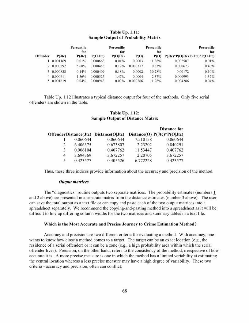
68

Table Up. 1.11:Sample Output of Probability Matrix

Percentilefor

Percentilefor

Percentilefor

Percentilefor

Offender P(Jtc) P(Jtc) P(O|Jtc) P(O|Jtc) P(O) P(O) P(Jtc)*P(O|Jtc) P(Jtc)*P(O|Jtc)

1 0.001169 0.01% 0.000663 0.01% 0.0003 11.38% 0.002587 0.01%

2 0.000292 5.68% 0.000483 0.12% 0.000377 0.33% 0.000673 0.40%

3 0.000838 0.14% 0.000409 0.18% 0.0002 30.28% 0.00172 0.10%

4 0.000611 1.56% 0.000525 1.47% 0.0004 2.37% 0.000993 1.37%5 0.001619 0.04% 0.000943 0.03% 0.000266 11.98% 0.004286 0.04%

Table Up. 1.12 illustrates a typical distance output for four of the methods. Only five serialoffenders are shown in the table.

Table Up. 1.12:Sample Output of Distance Matrix

Distance forOffenderDistance(Jtc) Distance(O|Jtc) Distance(O) P(Jtc)*P(O|Jtc)

1 0.060644 0.060644 7.510158 0.0606442 6.406375 0.673807 2.23202 0.8402913 0.906104 0.407762 11.53447 0.4077624 3.694369 3.672257 2.20705 3.6722575 0.423577 0.405526 6.772228 0.423577

Thus, these three indices provide information about the accuracy and precision of the method.

Output matrices

The “diagnostics” routine outputs two separate matrices. The probability estimates (numbers 1and 2 above) are presented in a separate matrix from the distance estimates (number 3 above). The usercan save the total output as a text file or can copy and paste each of the two output matrices into aspreadsheet separately. We recommend the copying-and-pasting method into a spreadsheet as it will bedifficult to line up differing column widths for the two matrices and summary tables in a text file.

Which is the Most Accurate and Precise Journey to Crime Estimation Method?

Accuracy and precision are two different criteria for evaluating a method. With accuracy, onewants to know how close a method comes to a target. The target can be an exact location (e.g., theresidence of a serial offender) or it can be a zone (e.g., a high probability area within which the serialoffender lives). Precision, on the other hand, refers to the consistency of the method, irrespective of howaccurate it is. A more precise measure is one in which the method has a limited variability at estimatingthe central location whereas a less precise measure may have a high degree of variability. These twocriteria - accuracy and precision, often can conflict.

69

The following example is from Jessen (1978). Consider a target that one is trying to ‘hit’ (FigureUp. 1.20). The target can be a physical target, such as a dart board, or it can be a location in space, suchas the residence of a serial offender. One can think of three different ‘throwers’ or methods attempting tohit the center of target, the Bulls Eye. The throwers make repeated attempts to hit the target and the‘throws’ (or estimates from the method) can be evaluated in terms of accuracy and precision. In FigureUp. 1.21, the thrower is all over the dartboard. There is no consistency at all. However, if the center ofminimum distance (Cmd) is calculated, it is very close to the actual center of the target, the Bulls Eye. In this case, the thrower is accurate but not precise. That is, there is no systematic bias in the thrower’sthrows, but they are not reliable. This thrower is accurate (or unbiased) but not precise.

In Figure Up.1. 22, there is an opposite condition. In this case, the thrower is precise but notaccurate. That is, there is a systematic bias in the throws even though the throws (or method) arerelatively consistent. Finally, in Figure Up. 1.23, the thrower is both relatively precise and accurate asthe Cmd of the throws is almost exactly on the Bulls Eye.

One can apply this analogy to a method. A method produces estimates from a sample. For eachsample, one can evaluate how accurate is the method (i.e., how close to the target did it come) and howconsistent is it (how much of variability does it produce). Perhaps the analogy is not perfect because thethrower makes multiple throws whereas the method produces a single estimate. But, clearly, we want amethod that is both accurate and precise.

Measures of Accuracy and Precision

Much of the debate in the area of journey to crime estimation has revolved around argumentsabout the accuracy and precision of the method. Levine (2004) first raised the issue of accuracy byproposing distance from the location with the highest probability to the location where the offender livedas a measure of accuracy, and suggested that simple, centrographic measures were as accurate as moreprecise journey to crime methods in estimating this. Snook and colleagues confirmed this conclusion andshowed that human subjects could do as well as any of the algorithms (Snook, Zito, Bennell, and Taylor,2005; Snook, Taylor and Bennell, 2004). Canter, Coffey and Missen (2000), Canter (2003), and Rossmo(2000) have argued for an area of highest probability being the criterion for evaluating accuracy,indicating a ‘search cost’ or a ‘hit score’ with the aim being to narrow the search area to as small aspossible. Rich and Shivley (2004) compared different journey to crime/geographic profiling softwarepackages and concluded that there were at least five different criteria for evaluating accuracy andprecision - error distance, search cost/hit score, profile error distance, top profile area, and profileaccuracy. Rossmo (2005a; b) and Rossmo and Filer (2005) have critiqued these measures as being toosimple and have rejected error distance. Levine (2005) justified the use of error distance as beingfundamental to statistical error while acknowledging that an area measure is necessary, too. Paulsen(2007; 2006a; 2006b) compared different journey to crime/geographic profiling methods and argued thatthey are more or less were comparable to in terms of several criteria of accuracy, both error distance andsearch cost/hit score.

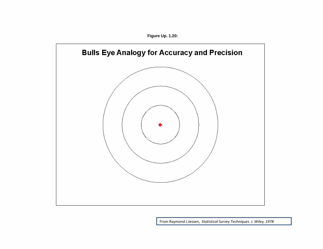
Figure Up. 1.20:

From Raymond J.Jessen,  Statistical Survey Techniques. J. Wiley, 1978

Figure Up. 1.21:

Figure Up. 1.22:

Figure Up. 1.23:

74

While the debate continues to develop, practically a distinction can be made in terms of measuresof accuracy and measures of precision. Accuracy is measured by how close to the target is the estimatewhile precision refers to how large or small an area the method produces. The two become identicalwhen the precision is extremely small, similar to a variance converging into a mean in statistics as thedistance between observations and the mean approach zero.

In evaluating the methods, five different measures are used:

Accuracy

1. True accuracy - the probability in the cell where the offender actually lives. TheBayesian Jtc diagnostics routine evaluates the six above mentioned methods on a sampleof serial offenders with known residence address. Each of the methods (except for thecenter of minimum distance, Cmd) has a probability distribution. That method whichhas the highest probability in the cell where the offender lives is the most accurate.

2. Diagnostic accuracy - the distance between the cell with the highest probability estimateand the cell where the offender lives. Each of the probability methods producesprobability estimates for each cell. The cell with the highest probability is the best guessof the method for where the offender lives. The error from this location to where theoffender lives is an indicator of the diagnostic accuracy of the method.

3. Neighborhood accuracy - the percent of offenders who reside within the cell with thehighest probability. Since the grid cell is the smallest unit of resolution, this measuresthe percent of all offenders who live at the highest probability cell. This was estimatedby those cases where the error distance was smaller than half the grid cell size.

Precision

4. Search cost/hit score - the percent of the total study area that has to be searched to findthe cell where the offender actually lived after having sorted the output cells from thehighest probability to the lowest

5. Potential search cost - the percent of offenders who live within a specified distance ofthe cell with the highest probability. In this evaluation, two distances are used thoughothers can certainly be used:

A. The percent of offender who live within one mile of the cell with the highestprobability.

B. The percent of offenders who live within one-half mile of the cell with thehighest probability (“Probable search area in miles”).

Summary Statistics

The “diagnostics” routine will also provide summary information at the bottom of each matrix. There are summary measures and counts of the number of times a method had the highest probability or

75

the closest distance from the cell with the highest probability to the cell where the offender actuallylived; ties between methods are counted as fractions (e.g., two tied methods are given 0.5 each; three tiedmethods are give 0.33 each). For the probability matrix, these statistics include:

1. The mean (probability or percentile);2. The median (probability or percentile);3. The standard deviation (probability or percentile);4. The number of times the P(Jtc) estimate produces the highest probility;5. The number of times the P(O|Jtc) estimate produces the highest probability;6. The number of times the P(O) estimate produces the highest probability;7. The number of times the product term estimate produces the highest probability;8. The number of times the Bayesian estimate produces the highest probability.

For the distance matrix, these statistics include:

1. The mean distance;2. The median distance;3. The standard deviation distance;4. The number of times the P(Jtc) estimate produces the closest distance;5. The number of times the P(O|Jtc) estimate produces the closest distance;6. The number of times the P(O) estimate produces the closest distance;7. The number of times the product term estimate produces the closest distance;8. The number of times the Bayesian estimate produces the closest distance; and9. The number of times the center of minimum distance produces the closest distance.

Testing the Routine with Serial Offenders from Baltimore County

To illustrate the use of the Bayesian Jtc diagnostics routine, the records of 88 serial offenderswho had committed crimes in Baltimore County, MD, between 1993 and 1997 were compiled into adiagnostics file. The number of incidents committed by these offenders varied from 3 to 33 and includeda range of different crime types (larceny, burglary, robbery, vehicle theft, arson, bank robbery). Thefollowing are the results for the three measures of accuracy and three measures of precision.

Because the methods are interdependent, traditional parametric statistical tests cannot be used. Instead, non-parametric tests have been applied. For the probability and distance measures, two testswere used. First, the Friedman two-way analysis of variance test examines differences in the overall rankorders of multiple measures (treatments) for a group of subjects (Kanji, 1993, 115; Siegel, 1956). This isa chi-square test and measures whether there are significant differences in the rank orders across allmeasures (treatments). Second, differences between specific pairs of measures can be tested using theWilcoxon matched pairs signed-ranks test (Siegel, 1956, 75-83). This examines pairs of methods by notonly their rank, but also by the difference in the values of the measurements.

For the percentage of offenders who live in the same grid cell, within one mile, and within onehalf-mile of the cell with the peak likelihood, the Cochran Q test for k related samples was used to testdifferences among the methods (Kanji, 1993, 74; Siegel, 1956, 161-166). This is a chi-square test ofwhether there are overall differences among the methods in the percentages, but it cannot indicatewhether any one method has a statistically higher percentage. Consequently, we then tested the method

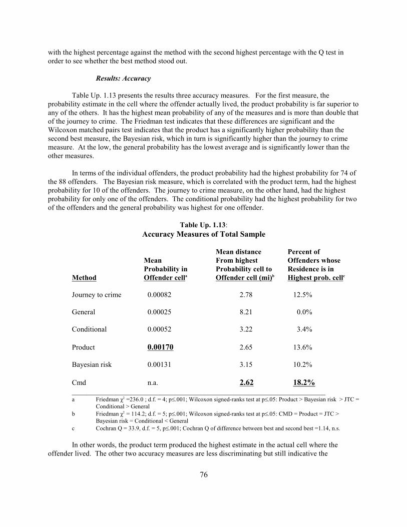
76

with the highest percentage against the method with the second highest percentage with the Q test inorder to see whether the best method stood out.

Results: Accuracy

Table Up. 1.13 presents the results three accuracy measures. For the first measure, theprobability estimate in the cell where the offender actually lived, the product probability is far superior toany of the others. It has the highest mean probability of any of the measures and is more than double thatof the journey to crime. The Friedman test indicates that these differences are significant and theWilcoxon matched pairs test indicates that the product has a significantly higher probability than thesecond best measure, the Bayesian risk, which in turn is significantly higher than the journey to crimemeasure. At the low, the general probability has the lowest average and is significantly lower than theother measures.

In terms of the individual offenders, the product probability had the highest probability for 74 ofthe 88 offenders. The Bayesian risk measure, which is correlated with the product term, had the highestprobability for 10 of the offenders. The journey to crime measure, on the other hand, had the highestprobability for only one of the offenders. The conditional probability had the highest probability for twoof the offenders and the general probability was highest for one offender.

Table Up. 1.13:

Accuracy Measures of Total Sample

Mean distance Percent ofMean From highest Offenders whoseProbability in Probability cell to Residence is in

Method Offender cell Offender cell (mi) Highest prob. cella b c

Journey to crime 0.00082 2.78 12.5%

General 0.00025 8.21 0.0%

Conditional 0.00052 3.22 3.4%

Product 0.00170 2.65 13.6%

Bayesian risk 0.00131 3.15 10.2%

Cmd n.a. 2.62 18.2%_____________________________________________________________________a Friedman ÷ =236.0 ; d.f. = 4; p£.001; Wilcoxon signed-ranks test at p£.05: Product > Bayesian risk > JTC =2

Conditional > Generalb Friedman ÷ = 114.2; d.f. = 5; p£.001; Wilcoxon signed-ranks test at p£.05: CMD = Product = JTC >2

Bayesian risk = Conditional < Generalc Cochran Q = 33.9, d.f. = 5, p£.001; Cochran Q of difference between best and second best =1.14, n.s.

In other words, the product term produced the highest estimate in the actual cell where theoffender lived. The other two accuracy measures are less discriminating but still indicative the

77

improvement gained from the Bayesian approach. For the measure of diagnostic accuracy (the distancefrom the cell with the highest probability to the cell where the offender lived), the center of minimumdistance (Cmd) had the lowest error distance followed closely by the product term. The journey to crimemethod had a slightly larger error. Again, the general probability had the greatest error, as might beexpected. The Friedman test indicates that there are overall differences in the mean distance among thesix measures. The Wilcoxon signed-ranks test, however, showed that the Cmd, the product, and thejourney to crime estimates are not significantly different, though all three are significantly lower than theBayesian risk measure and the conditional probability which, in turn, are significantly lower than thegeneral probability.

In terms of individual cases, the Cmd produced the lowest average error for 30 of the 88 caseswhile the conditional term (O|Jtc) had the lowest error in 17.9 cases (including ties). The product termproduced a lower average distance error for 9.5 cases (including ties) and the Jtc estimate produced loweraverage distance errors in 8.2 cases (again, including ties). In other words, the Cmd will either be veryaccurate or very inaccurate, which is not surprising given that it is only a point estimate.

Finally, for the third accuracy measure, the percent offenders residing in the area covered by thecell with the highest probability estimate, the Cmd has the highest percentage (18.2%) followed by theproduct probability, and the journey to crime probabilty. The Cochran Q shows that there are significantdifferences over all these measures. However, the difference between the measure with the highestpercentage in the same grid cell (the Cmd) and the measure with the second highest percentage (theproduct probability) is not significant.

For accuracy, the product probability appears to be better than the journey to crime estimate andalmost as accurate as the Cmd. It has the highest probability in the cell where the offender lived and alower error distance than the journey to crime (though not significantly so). Finally, it had a slightlyhigher percentage of offenders living in the area covered by cell with the highest probability than for thejourney to crime.

The Cmd, on the other hand, which had been shown to be the most accurate in previous studies(Levine, 2004; (Snook, Zito, Bennell, and Taylor, 2005; Snook, Taylor and Bennell, 2004; Paulsen,2006a; 2006b), does not appear to be more accurate than the product probability. It has only a slightlylower error distance and a slightly higher percentage of offenders residing in the area covered by the cellwith the highest probability. Thus, the product term has equaled the Cmd in terms of accuracy. Both,however, are more accurate than the journey to crime estimate.

Results: Precision

Table Up. 1.14 presents the three precision measures used to evaluate the six different measures. For the first measure, the mean percent of the study area with a higher probability (what Canter calls‘search cost’ and Rossmo calls ‘hit score’; Canter, 2003; Rossmo, 2005a, 2005b), the Bayesian riskmeasure had the lowest percentage followed closely by the product term. The conditional probabilitywas third followed by the journey to crime probability followed by the general probability. TheFriedman test indicates that these differences are significant overall and the Wilcoxon test shows that theBayesian risk, product term, conditional probability and journey to crime estimates are not significantlydifferent from each other. The general probability estimate, however, is much worse.

78

In terms of individual cases, the product probability had either the lowest percentage or was tiedwith other measures for the lowest percentage in 36 of the 88 cases. The Bayesian risk and journey tocrime measures had the lowest percentage or were tied with other measures for the lowest percentage in34 of the 88 cases. The conditional probability had the lowest percentage or was tied with other measuresfor the lowest percentage in 23 of the cases. Finally, the general probability had the lowest percentage orwas tied with other measures for the lowest percentage in only 7 of the cases.

Similar results are seen for the percent of offenders living within one mile of the cell with thehighest probability and also for the percent living within a half mile. For the percent within one mile, theproduct term had the highest percentage followed closely by the journey to crime measure and the Cmd. Again, at the low end is the general probability. The Cochran Q test indicates that these differences aresignificant over all measures though the difference between the best method (the product) and the secondbest (the journey to crime) is not significant.

Table Up. 1.14:

Precision Measures of Total Sample

Mean percent of Percent of offenders living withinStudy area with distance of highest probability cell:Higher

Method Probability 1 mile 0.5 milesa b c

Journey to crime 4.7% 56.8% 44.3%

General 16.8% 2.3% 0.0%

Conditional 4.6% 47.7% 31.8%

Product 4.2% 59.1% 48.9%

Bayesian risk 4.1% 51.1% 42.0%

Cmd n.a. 54.5% 42.0%________________________________________________________________a Friedman ÷ =115.4 ; d.f. = 4; p£.001; Wilcoxon signed-ranks test at p£.05: Bayesian risk =Product= JTC =2

Conditional> Generalb Cochran Q = 141.0, d.f. = 5, p£.001; Cochran Q of difference between best and second best = 0.7, n.s.c Cochran Q = 112.2, d.f. = 5, p£.001; Cochran Q of difference between best and second best = 2.0, n.s.

Conclusion of the Evaluation

In conclusion, the product method appears to be an improvement over the journey to crimemethod, at least with these data from Baltimore County. It is substantially more accurate and about asprecise. Further, the product probability appears to be, on average, as accurate as the Cmd, though theCmd still is more accurate for a small proportion of the cases (about one-sixth). That is, the Cmd willidentify about one-sixth of all offenders exactly. For a single guess of where a serial offender is living,the center of minimum distance produced the lowest distance error. But, since it is only a point estimate,

79

it cannot point to a search area where the offender might be living. The product term, on the other hand,produced an average distance error almost as small as the center of minimum distance, but producedestimates for other grid cells too. Among all the measures, it had the highest probability in the cell wherethe offender lived and was among the most efficient in terms of reducing the search area.

In other words, using information about the origin location of other offenders appears to improvethe accuracy of the Jtc method. The result is an index (the product term) that is almost as good as thecenter of minimum distance, but one that is more useful since the center of minimum distance is only asingle point.

Of course, each jurisdiction should re-run these diagnostics to determine the most appropriatemeasure. It is very possible that other jurisdictions will have different results due to the uniqueness oftheir land uses, street layout, and location in relation to the center of the metropolitan area. BaltimoreCounty is a suburb and the conclusions in a central city or in a rural area might be different.

Tests with Other Data Sets

The Bayesian Journey-to-crime model has been tested over the last few years in severaljurisdictions:

1. In Baltimore County with 850 serial offenders by Michael Leitner and Joshua Kent ofLouisiana State University (Leitner and Kent, 2009)

2. In the Hague, Netherlands with 62 serial burglars by Dick Block of Loyola University inChicago and Wim Bernasco of the Netherlands Institute for the Study of Crime and LawEnforcement (Block and Bernasco, 2009).

3. In Chicago, with 103 serial robbers by Dick Block of Loyola University (Levine andBlock, 2010).

4. In Manchester, England with 171 serial offenders by Patsy Lee of the GreaterManchester Police Department and myself (Levine and Lee, 2009)

In all cases, the product probability measures was both more accurate and more precise than theJourney to Crime measure. In two of the studies (Chicago and the Hague), the product term was alsomore accurate than the Center of Minimum Distance, the previous most accurate measure. In the othertwo studies (Baltimore County and Manchester), the Center of Minimum Distance was slightly moreaccurate than the product term. However, the product term has been more precise than the Center ofMinimum Distance in all four study comparisons. The mathematics of these models has been exploredby O’Leary (2009). These studies are presented in a special issue of the Journal of InvestigativePsychology and Offender Profiling. Introductions are provided by Canter (2009) and Levine (2009).

Estimate Likely Origin Location of a Serial Offender

The following applies to the Bayesian Jtc “Estimate likely origin of a serial offender” routine. Once the “diagnostic” routine has been run and a preferred method selected, the next routine allows theapplication of that method to a single serial offender.

80

Data Input

The user inputs the three required data sets and a reference file grid:

1. The incidents committed by a single offender that we’re interested in catching. Thismust be the Primary File;

2. A Jtc function that estimates the likelihood of an offender committing crimes at a certaindistance (or travel time if a network is used). This can be either a mathematically-defined function or an empirically-derived one (see Chapter 10 on Journey to CrimeEstimation). In general, the empirically-derived function is slightly more accurate thanthe mathematically-defined one (though the differences are not large);

3. An origin-destination matrix; and

4. The reference file also needs to be defined and should include all locations where crimeshave been committed (see Reference File).

Selected Method

The Bayesian Jtc “Estimate” routine interpolates the incidents committed by a serial offender toa grid, yielding an estimate of where the offender is liable to live. There are five different methods forthat can be used. However, the user has to choose one of these:

1. The Jtc distance method, P(Jtc);

2. The general crime distribution based on the origin-destination matrix, P(O). Essentially,this is the distribution of origins irrespective of the destinations;

3. The conditional Jtc distance. This is the distribution of origins based only on theincidents committed by other offenders in the same zones as those committed by theserial offender, P(O|Jtc). This is extracted from the O-D matrix;

4. The product of the Jtc estimate (1 above) and the distribution of origins based only onthe incidents committed by the serial offender (3 above), P(Jtc)*P(O|Jtc). This is thenumerator of the Bayesian function (equation Up. 1.38), the product of the priorprobability times the likelihood estimate; and

5. The Bayesian risk estimate as indicated in equation Up. 1.42 above (method 4 abovedivided by method 2 above), P(Bayesian).

Interpolated Grid

For the method that is selected, the routine overlays a grid on the study area. The grid is definedby the reference file parameters (see chapter 3). The routine then interpolates the input data set (theprimary file) into a probability estimate for each grid cell with the sum of the cells equaling 1.0 (withinthree decimal places). The manner in which the interpolation is done varies by the method chosen:

81

1. For the Jtc method, P(Jtc), the routine interpolates the selected distance function to eachgrid cell to produce a density estimate. The density estimates are converted toprobabilities so that the sum of the grid cells equals 1.0 (see chapter 10);

2. For the general crime distribution method, P(O), the routine sums up the incidents byeach origin zone and interpolates this to the grid using the normal distribution method ofthe single kernel density routine (see chapter 9). The density estimates are converted toprobabilities so that the sum of the grid cells equals 1.0;

3. For the distribution of origins based only on the incident committed by the serialoffender, the routine identifies the zone in which the incident occurs and reads only thoseorigins associated with those destination zones in the origin-destination matrix. Multipleincidents committed in the same origin zone are counted multiple times. The routinethen uses the single kernel density routine to interpolate the distribution to the grid (seechapter 9). The density estimates are converted to probabilities so that the sum of thegrid cells equals 1.0;

4. For the product of the Jtc estimate and the distribution of origins based only on theincidents committed by the serial offender , the routine multiples the probability estimateobtained in 1 above by the probability estimate obtained in 3 above. The productprobabilities are then re-scaled so that the sum of the grid cells equals 1.0; and

5. For the full Bayesian estimate as indicated in equation Up. 1.38 above, the routine takesthe product estimate (4 above) and divides it by the general crime distribution estimate (2above). The resulting density estimates are converted to probabilities so that the sum ofthe grid cells equals 1.0.

Note in all estimates, the results are then re-scaled so that the resulting grid is a probability (i.e.,all cells sum to 1.0).

Output

Once the method has been selected, the routine interpolates the data to the grid cell and outputs itas a ‘shp’, ‘mif/mid’, or Ascii file for display in a GIS program. The tabular output shows the probabilityvalues for each cell in the matrix and also indicates which grid cell has the highest probability estimate.

Accumulator Matrix

There is also an intermediate output, called the accumulator matrix, which the user can save. This lists the number of origins identified in each origin zone for the specific pattern of incidentscommitted by the offender, prior to the interpolation to grid cells. That is, in reading the origin-destination file, the routine first identifies which zone each incident committed by the offender fallswithin. Second, it reads the origin-destination matrix and identifies which origin zones are associatedwith incidents committed in the particular destination zones. Finally, it sums up the number of origins byzone ID associated with the incident distribution of the offender. This can be useful for examining thedistribution of origins by zones prior to interpolating these to the grid.

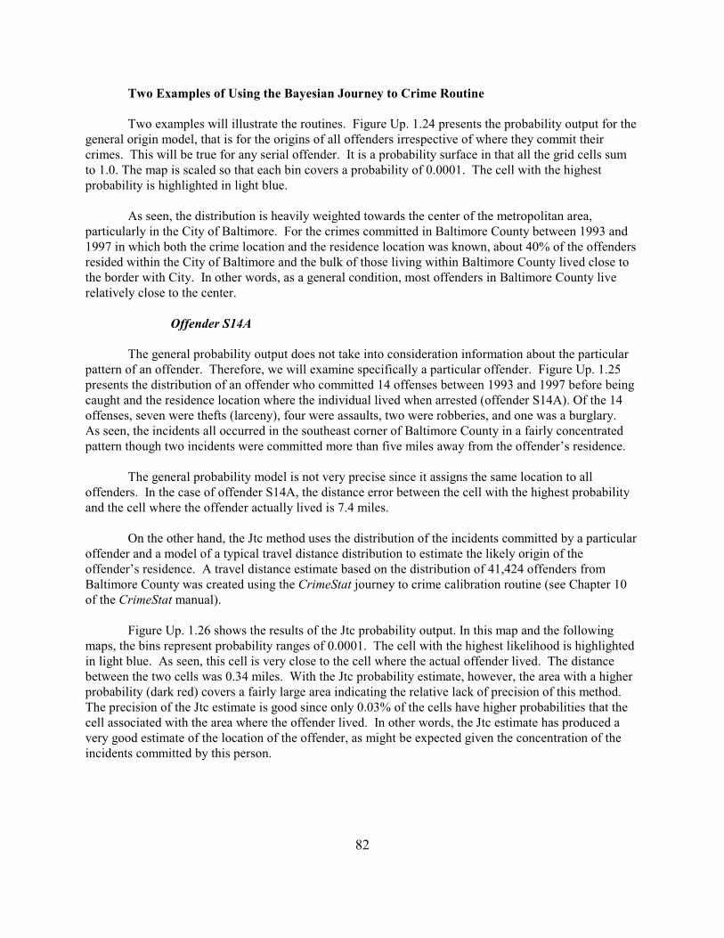
82

Two Examples of Using the Bayesian Journey to Crime Routine

Two examples will illustrate the routines. Figure Up. 1.24 presents the probability output for thegeneral origin model, that is for the origins of all offenders irrespective of where they commit theircrimes. This will be true for any serial offender. It is a probability surface in that all the grid cells sumto 1.0. The map is scaled so that each bin covers a probability of 0.0001. The cell with the highestprobability is highlighted in light blue.

As seen, the distribution is heavily weighted towards the center of the metropolitan area,particularly in the City of Baltimore. For the crimes committed in Baltimore County between 1993 and1997 in which both the crime location and the residence location was known, about 40% of the offendersresided within the City of Baltimore and the bulk of those living within Baltimore County lived close tothe border with City. In other words, as a general condition, most offenders in Baltimore County liverelatively close to the center.

Offender S14A

The general probability output does not take into consideration information about the particularpattern of an offender. Therefore, we will examine specifically a particular offender. Figure Up. 1.25presents the distribution of an offender who committed 14 offenses between 1993 and 1997 before beingcaught and the residence location where the individual lived when arrested (offender S14A). Of the 14offenses, seven were thefts (larceny), four were assaults, two were robberies, and one was a burglary. As seen, the incidents all occurred in the southeast corner of Baltimore County in a fairly concentratedpattern though two incidents were committed more than five miles away from the offender’s residence.

The general probability model is not very precise since it assigns the same location to alloffenders. In the case of offender S14A, the distance error between the cell with the highest probabilityand the cell where the offender actually lived is 7.4 miles.

On the other hand, the Jtc method uses the distribution of the incidents committed by a particularoffender and a model of a typical travel distance distribution to estimate the likely origin of theoffender’s residence. A travel distance estimate based on the distribution of 41,424 offenders fromBaltimore County was created using the CrimeStat journey to crime calibration routine (see Chapter 10of the CrimeStat manual).

Figure Up. 1.26 shows the results of the Jtc probability output. In this map and the followingmaps, the bins represent probability ranges of 0.0001. The cell with the highest likelihood is highlightedin light blue. As seen, this cell is very close to the cell where the actual offender lived. The distancebetween the two cells was 0.34 miles. With the Jtc probability estimate, however, the area with a higherprobability (dark red) covers a fairly large area indicating the relative lack of precision of this method. The precision of the Jtc estimate is good since only 0.03% of the cells have higher probabilities that thecell associated with the area where the offender lived. In other words, the Jtc estimate has produced avery good estimate of the location of the offender, as might be expected given the concentration of theincidents committed by this person.

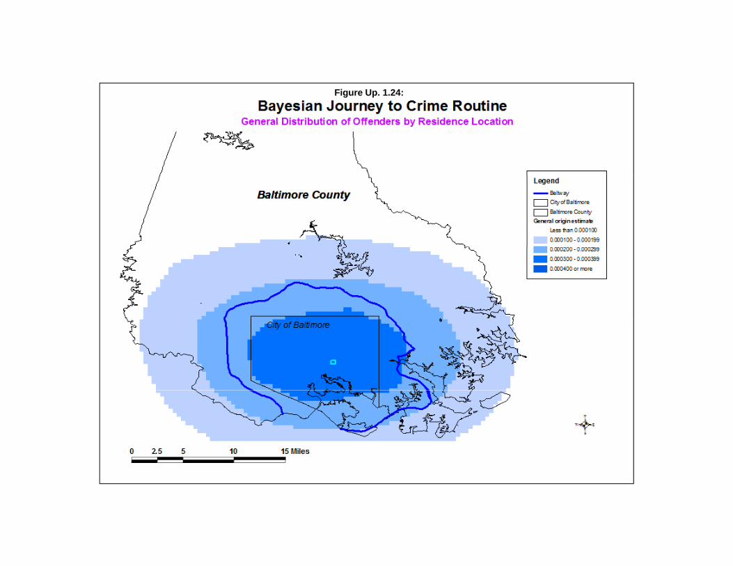
Figure Up. 1.24:

Figure Up. 1.25:

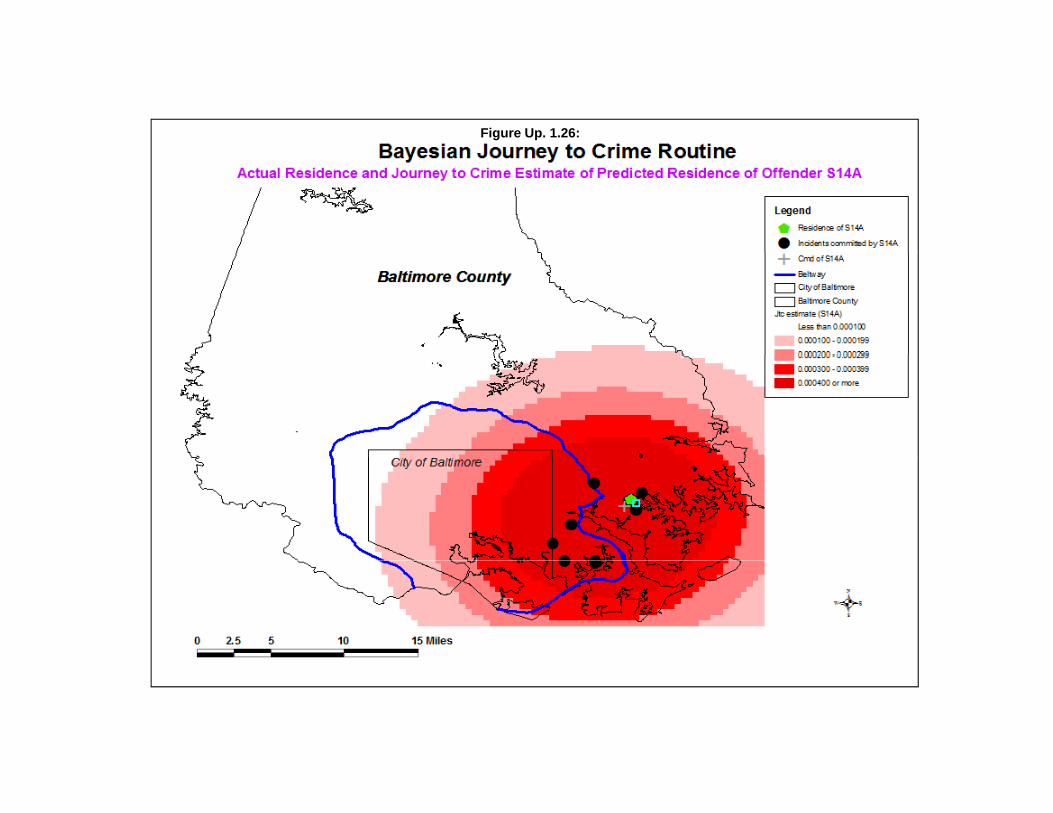
Figure Up. 1.26:

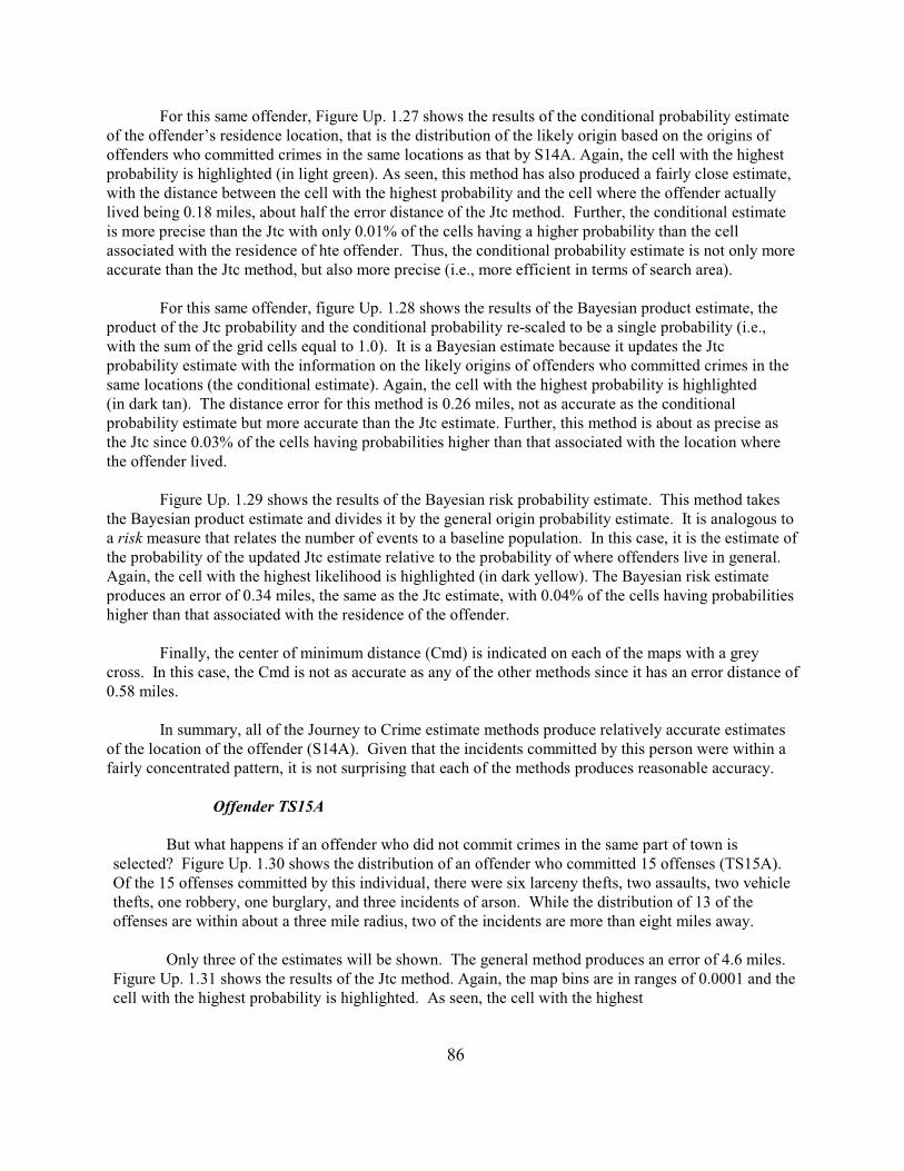
86

For this same offender, Figure Up. 1.27 shows the results of the conditional probability estimateof the offender’s residence location, that is the distribution of the likely origin based on the origins ofoffenders who committed crimes in the same locations as that by S14A. Again, the cell with the highestprobability is highlighted (in light green). As seen, this method has also produced a fairly close estimate,with the distance between the cell with the highest probability and the cell where the offender actuallylived being 0.18 miles, about half the error distance of the Jtc method. Further, the conditional estimateis more precise than the Jtc with only 0.01% of the cells having a higher probability than the cellassociated with the residence of hte offender. Thus, the conditional probability estimate is not only moreaccurate than the Jtc method, but also more precise (i.e., more efficient in terms of search area).

For this same offender, figure Up. 1.28 shows the results of the Bayesian product estimate, theproduct of the Jtc probability and the conditional probability re-scaled to be a single probability (i.e.,with the sum of the grid cells equal to 1.0). It is a Bayesian estimate because it updates the Jtcprobability estimate with the information on the likely origins of offenders who committed crimes in thesame locations (the conditional estimate). Again, the cell with the highest probability is highlighted (in dark tan). The distance error for this method is 0.26 miles, not as accurate as the conditionalprobability estimate but more accurate than the Jtc estimate. Further, this method is about as precise asthe Jtc since 0.03% of the cells having probabilities higher than that associated with the location wherethe offender lived.

Figure Up. 1.29 shows the results of the Bayesian risk probability estimate. This method takesthe Bayesian product estimate and divides it by the general origin probability estimate. It is analogous toa risk measure that relates the number of events to a baseline population. In this case, it is the estimate ofthe probability of the updated Jtc estimate relative to the probability of where offenders live in general.Again, the cell with the highest likelihood is highlighted (in dark yellow). The Bayesian risk estimateproduces an error of 0.34 miles, the same as the Jtc estimate, with 0.04% of the cells having probabilitieshigher than that associated with the residence of the offender.

Finally, the center of minimum distance (Cmd) is indicated on each of the maps with a greycross. In this case, the Cmd is not as accurate as any of the other methods since it has an error distance of0.58 miles.

In summary, all of the Journey to Crime estimate methods produce relatively accurate estimatesof the location of the offender (S14A). Given that the incidents committed by this person were within afairly concentrated pattern, it is not surprising that each of the methods produces reasonable accuracy.

Offender TS15A

But what happens if an offender who did not commit crimes in the same part of town isselected? Figure Up. 1.30 shows the distribution of an offender who committed 15 offenses (TS15A). Of the 15 offenses committed by this individual, there were six larceny thefts, two assaults, two vehiclethefts, one robbery, one burglary, and three incidents of arson. While the distribution of 13 of theoffenses are within about a three mile radius, two of the incidents are more than eight miles away.

Only three of the estimates will be shown. The general method produces an error of 4.6 miles. Figure Up. 1.31 shows the results of the Jtc method. Again, the map bins are in ranges of 0.0001 and thecell with the highest probability is highlighted. As seen, the cell with the highest

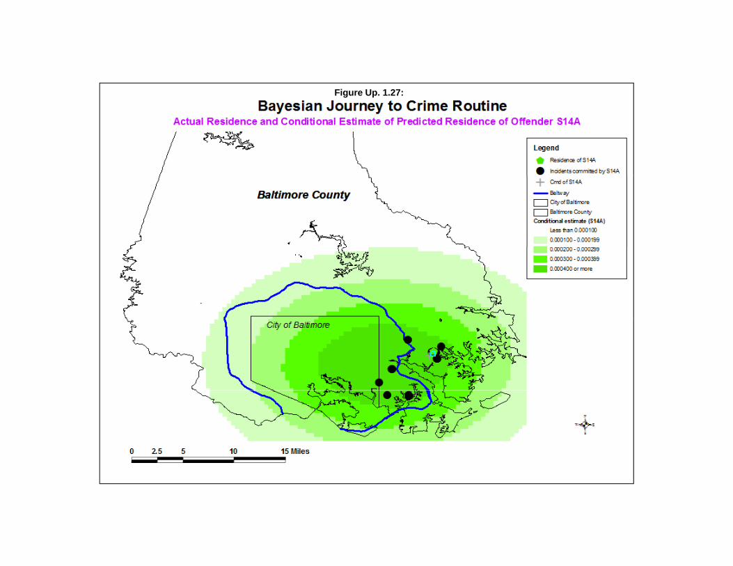
Figure Up. 1.27:

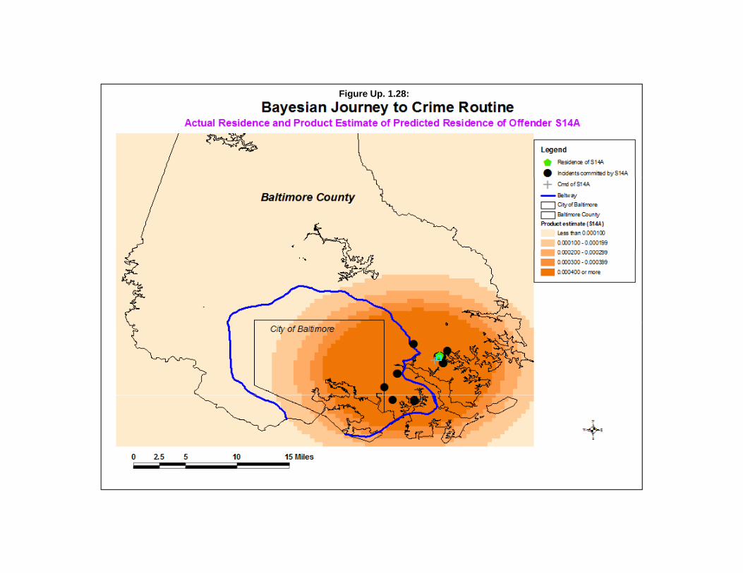
Figure Up. 1.28:

Figure Up. 1.29:

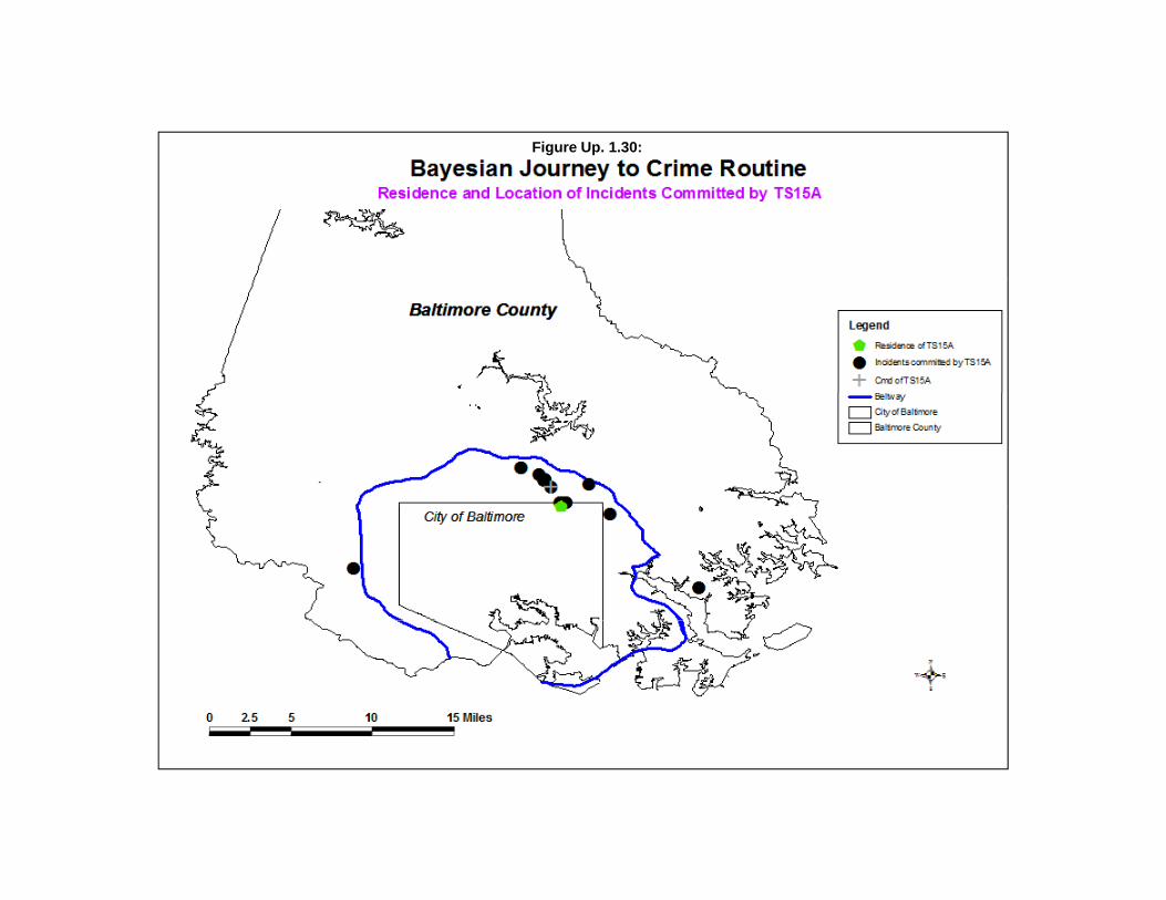
Figure Up. 1.30:

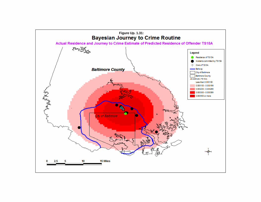
Figure Up. 1.31:

92

probability is located north and west of the actual offender’s residence. The distance error is 1.89 miles.The precision of this estimate is good with only 0.08% of the cells having higher probabilities than thecell where the offender lived.

Figure Up. 1.32 shows the result of the conditional probability estimate for this offender. In thiscase, the conditional probability method is less accurate than the Jtc method with a distance between thecell with the highest probability and the cell where the offender lived being 2.39 miles. However, thismethod is less precise than the Jtc method with 1.6% of the study area having probabilities higher thanthat in the cell where the offender lived.

Finally, figure Up. 1.33 shows the results of the product probability estimate. For this method,the error distance is only 0.47 miles, much less than the Jtc method. Further, it is smaller than thecenter of minimum distance which has a distance error of 1.33 miles. Again, updating the Jtc estimatewith information from the conditional estimate produces a more accurate guess where the offender lives. Further, the product estimate is more precise with only 0.02% of the study area having probabilitieshigher than the cell covering the area where the offender lived.

In other words, the “Estimate likely origin of a serial offender” routine allows the estimation ofa probability grid based on a single selected method. The user must decide which probability method toselect and the routine then calculates that estimate and assigns it to a grid. As mentioned above, the“diagnostics” routine should be first run to decide on which method is most appropriate for yourjurisdiction. In these 88 cases, the Bayesian product estimate was the most accurate of all theprobability methods. But, it is not known whether it will be the most accurate for other jurisdictions. Differences in the balance between central-city and suburbs, the road network, and land uses maychange the travel patterns of offenders. However, so far, as mentioned above, in tests in four cities(Baltimore County, Chicago, the Hague, Manchester), the product estimate has consistently been betterthan the journey to crime estimate and almost as good, if not better, than the center of minimumdistance. Further, the product term appears to be more precise than the journey to crime method. Thecenter of minimum distance, while generally more accurate than other methods, has no probabilitydistribution; it is simply a point. Consequently, one cannot select a search area from the estimate.

Potential to Add More Information to Improve the Methodology

Further, it should be possible to add more information to this framework to improve theaccuracy and precision of the estimates. One obvious dimension that should be added is an opportunitymatrix, a distribution of targets that are crime attractions for offenders. Among these are conveniencestores, shopping malls, parking lots, and other types of land uses that attract offenders. It will benecessary to create a probability matrix for quantifying these attractions. Further, the opportunitymatrix would have to be conditional on the distribution of the crimes and on the distribution of originsof offenders who committed crimes in the same location. The Bayesian framework is a conditional onewhere factors are added to the framework but conditioned on the distribution of earlier factors, namely

P(Jtc|O) % P(Jtc)*P(O|Jtc)*P(A|O,Jtc) (Up. 1.43)

where A is the attractions (or opportunities), Jtc is the distribution of incidents, and O is the distributionof other offender origins. It will not be an easy task to estimate an opportunity matrix that is

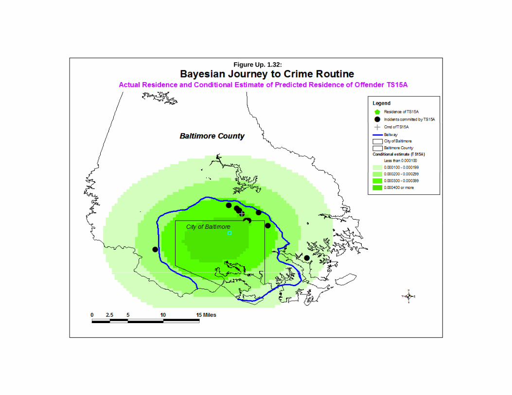
Figure Up. 1.32:

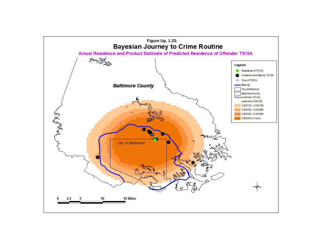
Figure Up. 1.33:

95

conditioned (dependent) upon both the distribution of offences (Jtc) and the origin of other offenderswho committed crimes in the same location (O|Jtc) and it may be necessary to approximate this througha series of filters.

Probability Filters

A filter is a probability matrix that is applied to the estimate but is not conditioned on theexisting variables in the model. For example, an opportunity matrix that was independent of thedistribution of offences by a single serial offender or the origins of other offenders who committedcrimes in the same locations could be applied as an alternative to equation Up. 1.43.

P(Jtc|O) % P(Jtc)*P(O|Jtc)*P(A) (Up. 1.44)

In this case, P(A) is an independent matrix. Another filter that could be applied are residentialland uses. The vast majority of offenders are going to live in residential areas. Thus, a residential landuse filter estimates the probability of a residential land use for every cell, P(Rs), could be applied toscreen out cells that are not residential, such as

P(Jtc|O) % P(Jtc)*P(O|Jtc)*P(A)*P(Rs) (Up. 1.45)

In this way, additional information can be integrated into the journey to crime methodology toimprove the accuracy and precision of the estimates. Clearly, having additional variables beconditioned upon existing variables in the model would be ideal since that would fit the true Bayesianapproach. But, even if independent filters were brought in, the model could be improved.

Summary

In sum, the Bayesian Jtc methodology presented here is an improvement over the currentjourney to crime method and appears to be as good, and more useful, than the center of minimumdistance. First, it adds new information to the journey to crime function to yield a more accurate andmore precise estimate. Second, it can sometimes predict the origin of ‘commuter’-type serial offenders,those individuals who do not commit crimes in their neighborhoods (Paulsen, 2007). The traditionaljourney to crime function cannot predict the origin location of a ‘commuter’-type. Of course, this willonly work if there are prior offenders who lived in the same location as the serial offender of interest. Ifthe offender lives in a neighborhood where there has been no previous serial offenders that aredocumented in the origin-destination matrix, the Bayesian approach cannot detect that location, either.

A caveat should be noted, however, in that the Bayesian method still has a substantial amount oferror. Much of this error reflects, I believe, the inherent mobility of offenders, especially those living ina suburb such as in Baltimore County. While adolescent offenders tend to commit crimes within a morecircumscribed area, the ability of an adult to own an automobile and to travel outside the residentialneighborhood is turning crime into a much more mobile phenomena than it was, say, 50 years ago whenonly about half of American households owned an automobile.

Thus, the Bayesian approach to Journey to Crime estimation must be seen as a tool whichproduces an incremental improvement in accuracy and precision. Geographic profiling is but one toolin the arsenal of methods that police must use to catch serial offenders.

96

References

Anselin, Luc (2008). “Personal note on the testing of significance of the local Moran values”.

Block, Richard and Wim Bernasco (2009). “Finding a serial burglar’s home using distance decay andconditional origin-destination patterns: A test of Empirical Bayes journey to crime estimation in TheHague”. Journal of Investigative Psychology & Offender Profiling. 6(3), 187-211.

Canter, David (2009). “Developments in geographical offender profiling: Commentary on Bayesianjourney-to-crime modeling”. Journal of Investigative Psychology & Offender Profiling. 6(3), 161-166.

Canter, David (2003). Dragnet: A Geographical Prioritisation Package. Center for InvestigativePsychology, Department of Psychology, The University of Liverpool: Liverpool, UK.http://www.i-psy.com/publications/publications_dragnet.php.

Canter, D., Coffey, T., Huntley, M., & Missen, C. (2000). “Predicting serial killers' home base using adecision support system”. Journal of Quantitative Criminology, 16 (4), 457 -- 478.

Canter, D. and A. Gregory (1994). “Identifying the residential location of rapists”, Journal of theForensic Science Society, 34 (3), 169-175.

Chainey, Spencer and Jerry Ratcliffe (2005). GIS and Crime Mapping, John Wiley & Sons,Inc.:Chichester, Sussex, England.

Denison, D.G.T., C.C. Holmes, B.K. Mallilck, and A.F.M. Smith (2002). Bayesian Methods forNonlinear Classification and Regression. John Wiley & Sons, Ltd: New York.

Gelman, Andrew, John B. Carlin, Hal S. Stern, and Donald B. Rubin (2004). Bayesian Data Analysis(second edition). Chapman & Hall/CRC: Boca Raton, FL

Getis, A. and J.K. Ord (1992). “The analysis of spatial association by use of distance statistics”,Geographical Analysis, 24, 189-206.

Hansen, Katherine (1991). “Head-banging: robust smoothing in the plane”. IEEE Transactions onGeoscience and Remote Sensing, 29 (3), 369-378.

Kanji, Gopal K. (1993). 100 Statistical Tests. Sage Publications: Thousand Oaks, CA.

Khan, Ghazan, Xiao Qin, and David A. Noyce (2006). “Spatial analysis of weather crash patterns inWisconsin”. 85 Annual meeting of the Transportation Research Board: Washington, DC.th

Lee, Jay and David W. S. Wong (2001). Statistical Analysis with ArcView GIS. J. Wiley & Sons, Inc.:New York.

Lee, Peter M. (2004). Bayesian Statistics: An Introduction (third edition). Hodder Arnold: London.

97

Lees, Brian (2006). “The spatial analysis of spectral data: Extracting the neglected data”, Applied GIS, 2(2), 14.1-14.13.

Leitner, Michael and Joshua Kent (2009). “Bayesian journey to crime modeling of single- and multiplecrime type series in Baltimore County, MD”. Journal of Investigative Psychology & Offender Profiling. 6(3), 213-236.

Levine, Ned, and Richard Block (2010). Bayesian Journey-to-Crime Estimation: An Improvement inGeographic Profiling Methodology”. The Professional Geographer. In press.

Levine, Ned and Patsy Lee (2009). “Bayesian journey to crime modeling of juvenile and adultoffenders by gender in Manchester”. Journal of Investigative Psychology & Offender Profiling. 6(3),237-251.

Levine, Ned (2009). “Introduction to the special issue on Bayesian Journey-to-crime modeling”.Journal of Investigative Psychology & Offender Profiling. 6(3), 167-185.

Levine, Ned (2005). “The evaluation of geographic profiling software: Response to Kim Rossmo'scritique of the NIJ methodology”. http://www.nedlevine.com/Response to Kim Rossmo Critique of theGP Evaluation Methodology.May 8 2005.doc

Levine, Ned (2004). “Journey to crime Estimation”. Chapter 10 of Ned Levine (ed), CrimeStat III: ASpatial Statistics Program for the Analysis of Crime Incident Locations (version 3.0). Ned Levine &Associates, Houston, TX.; National Institute of Justice, Washington, DC. November.http://www.icpsr.umich.edu/crimestat. Originally published August 2000.

Mungiole, Michael, Linda W. Pickle, and Katherine H. Simonson (2002). “Application of a weightedHead-Banging algorithm to Mortality data maps”, Statistics in Medicine, 18, 3201-3209.

Mungiole, Michael and Linda Williams Pickle (1999). “Determining the optimal degree of smoothingusing the weighted head-banging algorithm on mapped mortality data”, In ASC '99 - Leading Survey &Statistical Computing into the New Millennium, Proceedings of the ASC International Conference,September. Available at http://srab.cancer.gov/headbang.

O’Leary, Mike (2009). “The mathematics of geographical profiling”. Journal of InvestigativePsychology & Offender Profiling. 6(3), 253-265.

Ord, J.K. and A. Getis (1995). “Local spatial autocorrelation statistics:Distributional Issues and anApplication. Geographical Analysis, Vol. 27, 1995, 286-306.

Paulsen, Derek (2007). “Improving geographic profiling through commuter/marauder prediction:. Police Practice and Research 8: 347-357

Paulsen, Derek (2006a). “Connecting the dots: assessing the accuracy of geographic profilingsoftware”. Policing: An International Journal of Police Strategies and Management. 20 (2), 306-334.

98

Paulsen, Derek (2006b). “Human versus machine: A comparison of the accuracy of geographic profilingmethods”. Journal of Investigative Psychology and Offender Profiling 3: 77-89.

Pickle, Linda W. and Yuchen Su (2002). “Within-State geographic patterns of health insurancecoverage and health risk factors in the United States”, American Journal of Preventive Medicine, 22 (2),75-83.

Pickle, Linda Williams, Michael Mungiole, Gretchen K Jones, Andrew A White (1996). Atlas of UnitedStates Mortality. National Center for Health Statistics: Hyattsville, MD.

Rich, T., & Shively, M. (2004). A Methodology for Evaluating Geographic Profiling Software. FinalReport for the National Institute of Justice, Abt Associates: Cambridge, MA.http://www.ojp.usdoj.gov/nij/maps/gp.pdf

Rossmo, D. Kim (2005a). “Geographic heuristics or shortcuts to failure?: Response to Snook et al.Applied Cognitive Psychology 19: 651-654.

Rossmo, D. Kim (2005b). “Response to NIJ’s methodology for evaluating geographic profilingsoftware”. http://www.ojp.usdoj.gov/nij/maps/gp.htm.

Rossmo, D. Kim, & Filer, S. (2005). “Analysis versus guesswork”. Blue Line Magazine, , August /September, 24:26.

Rossmo, D. Kim (2000). Geographic Profiling. CRC Press: Boca Raton Fl.

Rossmo, D. Kim (1995). “Overview: multivariate spatial profiles as a tool in crime investigation”. InCarolyn Rebecca Block, Margaret Dabdoub and Suzanne Fregly, Crime Analysis Through ComputerMapping. Police Executive Research Forum: Washington, DC. 65-97.

Siegel, Sidney (1956). Nonparametric Statistics for the Behavioral Sciences. McGraw-Hill: NewYork.

Snook, Brent, Michele Zito, Craig Bennell, and Paul J. Taylor (2005). “On the complexity and accuracyof geographic profiling strategies”. Journal of Quantitative Criminology, 21 (1), 1-26.

Snook, Brent, Paul Taylor and Craig Bennell (2004). “Geographic profiling; the fast, fugal and accurateway”. Applied Cognitive Psychology 18: 105-121.

Tukey, P. A. and J.W. Tukey (1981). “Graphical display of data sets in 3 or more dimensions”. In V.Barnett (ed), Interpreting Multivariate Data. John Wiley & Sons: New York.

Wikipedia (2007a). “Geometric mean” http://en.wikipedia.org/wiki/Geometric_mean and “Weightedgeometric mean” http://en.wikipedia.org/wiki/Weighted_geometric_mean.

Wikipedia (2007b). “Harmonic mean” http://en.wikipedia.org/wiki/Harmonic_mean and “Weightedharmonic mean” http://en.wikipedia.org/wiki/Weighted_harmonic_mean.