Embed Size (px)
Citation preview
FACULTEIT Ingenieurswetenschappen
Eindwerk ingediend voor het behalen van de graad van Master in de Ingenieurswetenschappen: Toegepaste Computerwetenschappen
Cross-layer Link Estimation For Contiki-based Wireless Sensor Networks Ward Van Heddeghem Promotor: Prof. Dr. ir. Kris Steenhaut Copromotor: Prof. Dr. Ann Nowé Begeleider: ir. Joris Borms
Academiejaar 2008-2009

ii
iii
Abstract
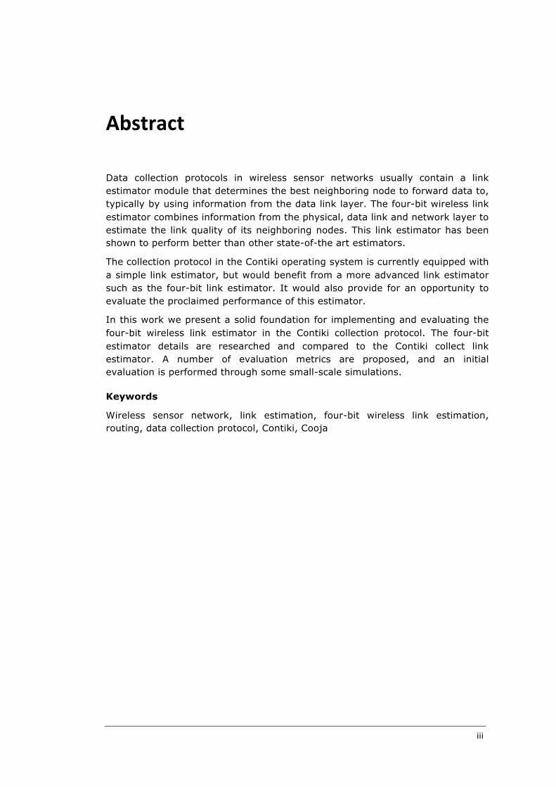
Data collection protocols in wireless sensor networks usually contain a link estimator module that determines the best neighboring node to forward data to, typically by using information from the data link layer. The four-bit wireless link estimator combines information from the physical, data link and network layer to estimate the link quality of its neighboring nodes. This link estimator has been shown to perform better than other state-of-the art estimators.
The collection protocol in the Contiki operating system is currently equipped with a simple link estimator, but would benefit from a more advanced link estimator such as the four-bit link estimator. It would also provide for an opportunity to evaluate the proclaimed performance of this estimator.
In this work we present a solid foundation for implementing and evaluating the four-bit wireless link estimator in the Contiki collection protocol. The four-bit estimator details are researched and compared to the Contiki collect link estimator. A number of evaluation metrics are proposed, and an initial evaluation is performed through some small-scale simulations.
Keywords
Wireless sensor network, link estimation, four-bit wireless link estimation, routing, data collection protocol, Contiki, Cooja
iv
Abstract
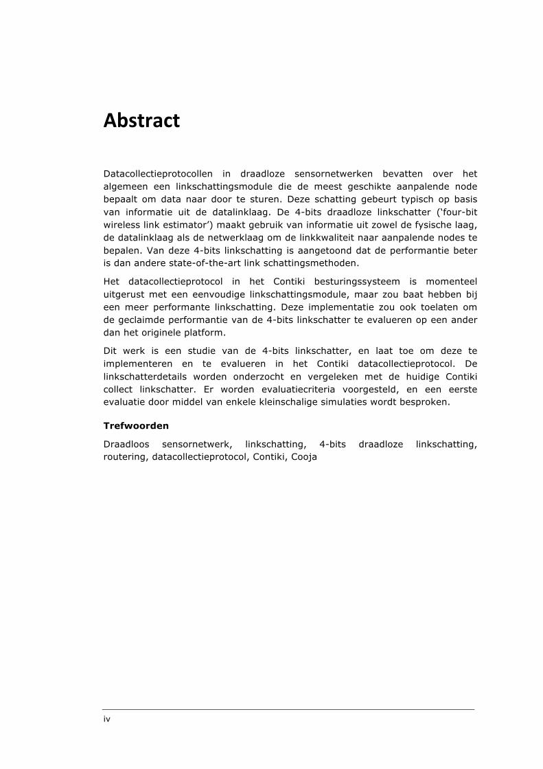
Datacollectieprotocollen in draadloze sensornetwerken bevatten over het algemeen een linkschattingsmodule die de meest geschikte aanpalende node bepaalt om data naar door te sturen. Deze schatting gebeurt typisch op basis van informatie uit de datalinklaag. De 4-bits draadloze linkschatter (‘four-bit wireless link estimator’) maakt gebruik van informatie uit zowel de fysische laag, de datalinklaag als de netwerklaag om de linkkwaliteit naar aanpalende nodes te bepalen. Van deze 4-bits linkschatting is aangetoond dat de performantie beter is dan andere state-of-the-art link schattingsmethoden.
Het datacollectieprotocol in het Contiki besturingssysteem is momenteel uitgerust met een eenvoudige linkschattingsmodule, maar zou baat hebben bij een meer performante linkschatting. Deze implementatie zou ook toelaten om de geclaimde performantie van de 4-bits linkschatter te evalueren op een ander dan het originele platform.
Dit werk is een studie van de 4-bits linkschatter, en laat toe om deze te implementeren en te evalueren in het Contiki datacollectieprotocol. De linkschatterdetails worden onderzocht en vergeleken met de huidige Contiki collect linkschatter. Er worden evaluatiecriteria voorgesteld, en een eerste evaluatie door middel van enkele kleinschalige simulaties wordt besproken.
Trefwoorden
Draadloos sensornetwerk, linkschatting, 4-bits draadloze linkschatting, routering, datacollectieprotocol, Contiki, Cooja

v
Acknowledgments
I would like to thank a number of people for their help and support.
First, I would like to thank Prof. Dr. ir. Kris Steenhaut who gave me the opportunity to work on such an interesting topic and kept me on track with regular deadlines.
I would like to thank Joris Borms for his guidance and advice. I would like to thank Bart Lemmens for taking the time to read this work through, and Walter Colitti for organizing insightful meetings.
Also, I would like to thank Jelmer Tiete, who helped me out trying to get things working on Sentilla nodes.
Finally, I am forever in debt to my girlfriend Klaske, who supported me when I took up studying again and did overtime as a fresh mother to let me work on my thesis.
Ward, May 2009

vi
vii
Tableofcontents
1 Introduction ......................................................................................11.1What it is about............................................................................. 11.2Goal of this work ........................................................................... 31.3Outline and contributions of this work .............................................. 4
2 Background .......................................................................................52.1Wireless mesh networks ................................................................. 5
2.1.1 Categorizing networks .......................................................... 52.1.2 Multi-hop wireless networks .................................................. 5
2.2Wireless Sensor Networks............................................................... 62.3 Collection protocols & link estimators ............................................... 72.4 The Contiki operating system .......................................................... 9
2.4.1 Overview ............................................................................ 92.4.2 The Rime stack.................................................................. 102.4.3 The announcement primitive ............................................... 11
2.5 The Contiki collect protocol ........................................................... 122.5.1 Components...................................................................... 132.5.2 Protocol attributes ............................................................. 172.5.3 Operation (initialization, sending and receiving) ..................... 18
2.6 The four-bit wireless link estimator (4B) ......................................... 203 Implementation of 4B......................................................................23
3.1Where does 4B fit in? ................................................................... 233.2 The 4B hybrid estimator algorithm ................................................. 23
3.2.1 Neighbor insertion (neighbor table management) ................... 263.2.2 Link quality calculation ....................................................... 27
3.3 Implementation notes .................................................................. 283.4 Rewrite of the Rime reliable unicast primitive .................................. 29
3.4.1 The problem ..................................................................... 293.4.2 The solution ...................................................................... 30
4 Evaluation of 4B ..............................................................................334.1 Introduction................................................................................ 334.2 Evaluation metrics ....................................................................... 334.3 Simulation .................................................................................. 34
4.3.1 Evaluation methods............................................................ 344.3.2 Parameters influencing the evaluation/simulation ................... 344.3.3 Setup and processing of the information ............................... 374.3.4 Simulation results .............................................................. 39
4.4 Evaluation .................................................................................. 444.4.1 Packet delivery cost (PDC) and delivery ratio (DR) ................. 44
viii
4.4.2 Memory requirements ........................................................ 444.4.3 Complexity ....................................................................... 45
4.5 Conclusion.................................................................................. 465 Thesis evaluation.............................................................................47
5.1 Thesis progress ........................................................................... 475.2 Problems encountered.................................................................. 47
6 Conclusion and further work............................................................496.1 Conclusion.................................................................................. 496.2 Further work............................................................................... 496.3Other suggestions........................................................................ 50
7 Literature ........................................................................................538 Appendix .........................................................................................55
8.1 Appendix A – Tutorial ‘Installing Contiki / Cooja on Ubuntu 8.10’ ....... 558.2 Appendix B – Tutorial ‘Getting started with Sentilla nodes’ ................ 598.3 Appendix C – Source code brunicast............................................... 66
8.3.1 brunicast.h ....................................................................... 668.3.2 brunicast.c........................................................................ 67
8.4 Appendix D – Source code 4B........................................................ 728.4.1 neighbor.h ........................................................................ 728.4.2 neighbor.c ........................................................................ 73
8.5 Appendix E – Reported bugs ......................................................... 86
ix
Tableoffigures
Figure 1 – A wireless sensor network setup for volcano monitoring (source: [13]).......................................................................................... 1
Figure 2 – The four-bit wireless link estimator and the OSI reference model ...... 2Figure 3 – A WSN Sentilla node as used at the VUB ....................................... 3Figure 4 – A multi-hop ‘mesh’ wireless network (source: [7]) ............................ 6Figure 5 – Different motes, each with a 8 MHz microcontroller, 10kB of
RAM, 48kB of program flash, and a 250kbps radio (source: [11]) ....... 7Figure 6 – A sample collection tree, showing per-link and node costs. The
cost of a node is its next hop’s cost plus the cost of the link (source: [11]) ............................................................................. 8
Figure 7 – Cooja, the network simulator that comes with Contiki ................... 10Figure 8 – The communication primitives in the Rime stack........................... 11Figure 9 – The polite-announcement algorithm............................................ 12Figure 10 – The Contiki collect protocol: event processing............................. 13Figure 11 – The Contiki collect protocol: link estimator and neighbor
management........................................................................... 16Figure 12 – 4B mapped to the Rime protocol stack ...................................... 21Figure 13 – The 4B link estimator .............................................................. 25Figure 14 – The 4B link estimator – neighbor insertion ................................. 26Figure 15 – The 4B link estimator – link quality calculation ........................... 27Figure 16 – Example hybrid ETX calculation (source: [8])............................... 28Figure 17 – The brunicast (better runicast) primitive that replaced the
flawed runicast and stunicast primitives ...................................... 30Figure 18 – Evaluation setup..................................................................... 37Figure 19 – Information logging ................................................................ 38Figure 20 – Final collection routing tree after 720 seconds ............................ 39Figure 21 – Node metric evolution during the simulation............................... 40Figure 22 – PDC and DR........................................................................... 41Figure 23 – Retransmission count .............................................................. 42Figure 24 – Bad ACK count ....................................................................... 42Figure 25 – How bad ACKs occur at link-level .............................................. 43Figure 26 – Mockup of Cooja log visualized in an event-diagram .................... 50Figure 27 – Collection tree visualization example ......................................... 51

x
1 - Introduction 1
1 Introduction
1.1 Whatitisabout
If you do not happen to be active in a telecom related research field, chances are fairly small that you have ever heard of wireless sensor networks (WSNs). A wireless sensor network is exactly what its name implies; it is a network of small devices which each contain a sensor (to measure for example temperature, or pressure, or both), and which communicate with each other wirelessly.
WSNs have come into existence only about a decade ago. As often the case, their birth was inspired by military motives, where the idea of so-called ‘smart dust’ was proposed. As the story goes, smart dust is a collection of tiny, dust-sized devices that can be sprinkled by an airplane over hostile territory. Once deployed, these devices start gathering tactical data such as troop movements, and transmit this data from one device to another until it happens to reach some sort of collection point – for example a computer in a scouting vehicle – were the data can be collect and further analyzed.
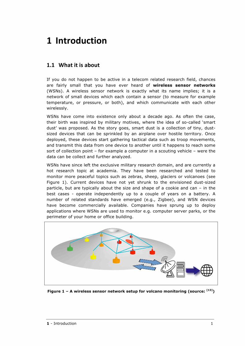
WSNs have since left the exclusive military research domain, and are currently a hot research topic at academia. They have been researched and tested to monitor more peaceful topics such as zebras, sheep, glaciers or volcanoes (see Figure 1). Current devices have not yet shrunk to the envisioned dust-sized particle, but are typically about the size and shape of a cookie and can – in the best cases - operate independently up to a couple of years on a battery. A number of related standards have emerged (e.g., Zigbee), and WSN devices have become commercially available. Companies have sprung up to deploy applications where WSNs are used to monitor e.g. computer server parks, or the perimeter of your home or office building.
Figure 1 – A wireless sensor network setup for volcano monitoring (source: [13])
2 1 - Introduction
Still, a lot of WSN research is going on. The quest to prolong the independent operation of these battery-powered devices fuels research for new ways to limit the energy consumption, which is primarily defined by the radio communication between the devices. Also, novel ways are researched to transfer the data in the most optimal way (i.e. requiring the least energy) to a nearby collection point.
One such research topic focuses on the way in which a device selects the optimal neighbor to send its data to. Out of the potentially many neighboring devices it can communicate with and set up a link, it has to estimate which link is the best one. The component of the routing algorithm that decides upon this is called a link estimator.
Initial link estimators were relatively simple and selected the neighbor that led to the collection point with the fewest number of hops (i.e. jumps from device to device). A number of improved link estimators have been proposed, a recent one being called four-bit wireless link estimator (4B), and subject of this work.
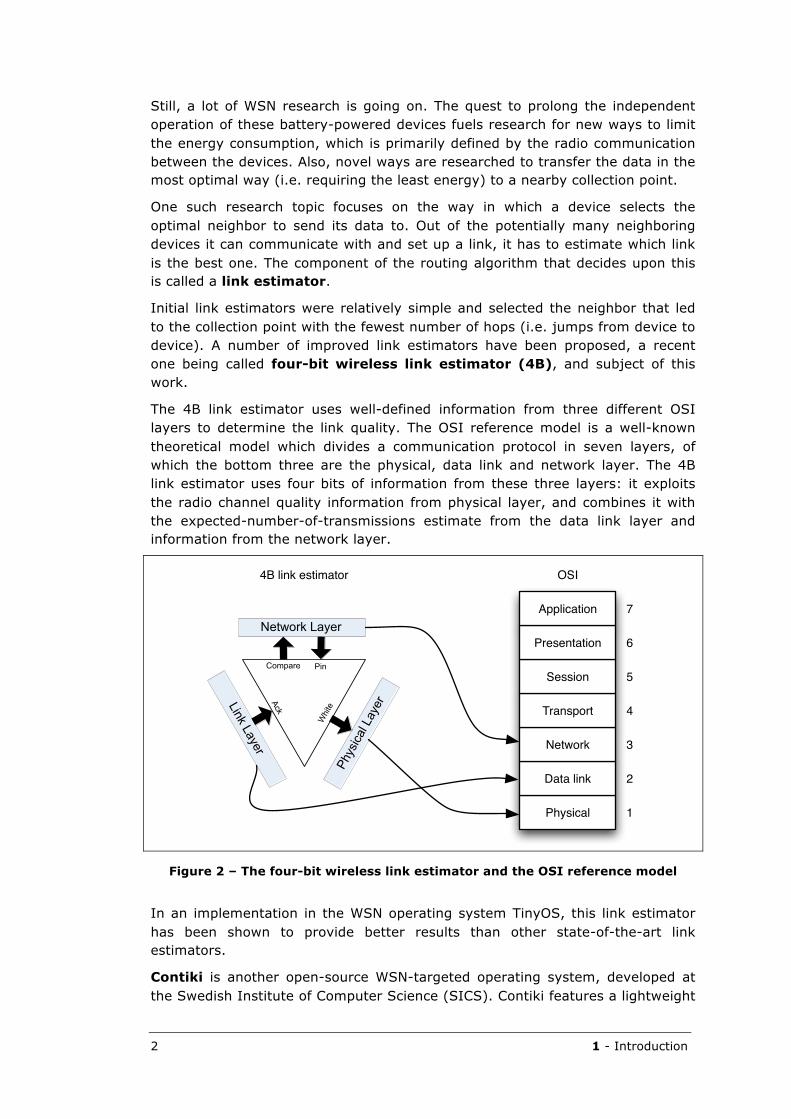
The 4B link estimator uses well-defined information from three different OSI layers to determine the link quality. The OSI reference model is a well-known theoretical model which divides a communication protocol in seven layers, of which the bottom three are the physical, data link and network layer. The 4B link estimator uses four bits of information from these three layers: it exploits the radio channel quality information from physical layer, and combines it with the expected-number-of-transmissions estimate from the data link layer and information from the network layer.
Figure 2 – The four-bit wireless link estimator and the OSI reference model
In an implementation in the WSN operating system TinyOS, this link estimator has been shown to provide better results than other state-of-the-art link estimators.
Contiki is another open-source WSN-targeted operating system, developed at the Swedish Institute of Computer Science (SICS). Contiki features a lightweight
Physical
Data link
Network
Transport
Session
Presentation
Application
1
2
3
4
5
6
7
OSI4B link estimator

1 - Introduction 3
network stack called Rime that provides, among other things, a data collection protocol to route data to a collection device. This collection protocol has a simple link estimator based on information solely from the data link layer.
It has been deemed useful by SICS to incorporate the 4B link estimator in Contiki, both to validate (or refute) the improved performance of this estimator, as well as to equip the collection protocol with a better link estimator.
Since the VUB TELE research group is also active on Contiki-based WSN research, and since a testbed of Sentilla nodes (see Figure 3) is available to run experiments on, this research project was a perfect fit.
Figure 3 – A WSN Sentilla node as used at the VUB
1.2 Goalofthiswork
As it was realized during this work that the original 4B paper[8] was not as detailed as initially assumed, the goal of this work is to study the details and application domain of the 4B link estimator as to provide a solid foundation for a future implementation and evaluation of 4B.
Personal motivation
On a personal level, I was interested in doing this thesis for a number of reasons. I think they are equally important for stating here, since they, as well, shape the setup and content of this thesis:
• I believe that for any student in the field of computer science, it is of great value to have some practical experience with the C programming language. Not only for adding an extra language to one’s toolkit, but also since C exposes some of the lower level details when interfacing with hardware, thereby providing a lot of insight. Since I had no practical experience programming in C, I deemed it important to do so before graduating.
• I am interested in networking and the co-operation of distributed systems. Wireless sensor networks provide a fascinating blend of both these topics. This thesis provides me with the opportunity to get hands-on experience and contact with networking stacks.

4 1 - Introduction
• The Contiki operating system is a relatively young but very vibrant, fast-moving research project. It is rewarding to try to contribute to such a project.
1.3 Outlineandcontributionsofthiswork
Research contributions
This work provides a solid foundation for the implementation and evaluation of the four-bit wireless link estimator in Contiki:
• After a short introduction to wireless sensor networks (§ 2.2) and showing the relevance of link estimators in collection protocols (§ 2.3), we completely dissect and document the current Contiki data collection protocol (§ 2.5). This information is based on a detailed study of the Contiki source code.
• We completely dissect and document the 4B wireless link estimator (§ 3), discussing the differences with the Contiki collect estimator. This study is then used for an initial, working implementation in Contiki (§ 3.3).
• Finally, we propose a number of evaluation metrics (§ 4.2), investigate evaluation conditions (§ 4.3.2), and perform some small-scale simulation experiments.
Community contributions
Additionally, this work also resulted in a number of minor contributions to the Contiki community:
• To alleviate the problem of lack of documentation, two tutorials were created and published on the Contiki website. The first tutorial (see § 8.1) describes in detail the installation process of Contiki and Cooja on Ubuntu. The second tutorial (see § 8.2) is more extensive and describes ‘getting started with Sentilla nodes’.
• A number of bugs were discovered and reported to the Contiki mailing list (see § 8.5).
• The reliable unicast primitive brunicast (see § 3.4) was submitted for replacement of runicast and stunicast in the Rime stack.
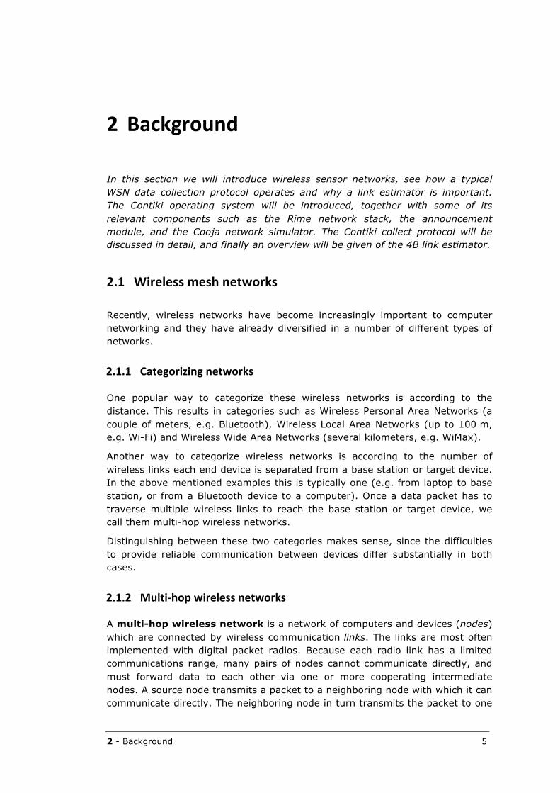
2 - Background 5
2 Background
In this section we will introduce wireless sensor networks, see how a typical WSN data collection protocol operates and why a link estimator is important. The Contiki operating system will be introduced, together with some of its relevant components such as the Rime network stack, the announcement module, and the Cooja network simulator. The Contiki collect protocol will be discussed in detail, and finally an overview will be given of the 4B link estimator.
2.1 Wirelessmeshnetworks
Recently, wireless networks have become increasingly important to computer networking and they have already diversified in a number of different types of networks.
2.1.1 Categorizingnetworks
One popular way to categorize these wireless networks is according to the distance. This results in categories such as Wireless Personal Area Networks (a couple of meters, e.g. Bluetooth), Wireless Local Area Networks (up to 100 m, e.g. Wi-Fi) and Wireless Wide Area Networks (several kilometers, e.g. WiMax).
Another way to categorize wireless networks is according to the number of wireless links each end device is separated from a base station or target device. In the above mentioned examples this is typically one (e.g. from laptop to base station, or from a Bluetooth device to a computer). Once a data packet has to traverse multiple wireless links to reach the base station or target device, we call them multi-hop wireless networks.
Distinguishing between these two categories makes sense, since the difficulties to provide reliable communication between devices differ substantially in both cases.
2.1.2 Multi‐hopwirelessnetworks
A multi-hop wireless network is a network of computers and devices (nodes) which are connected by wireless communication links. The links are most often implemented with digital packet radios. Because each radio link has a limited communications range, many pairs of nodes cannot communicate directly, and must forward data to each other via one or more cooperating intermediate nodes. A source node transmits a packet to a neighboring node with which it can communicate directly. The neighboring node in turn transmits the packet to one
6 2 - Background
of its neighbors, and so on until the packet is transmitted to its ultimate destination. Each link that a packet is sent over is referred to as a hop; the set of links that a packet travels over from the source to the destination is called a route or path. Routes are discovered by running a distributed routing protocol on the network.[7]
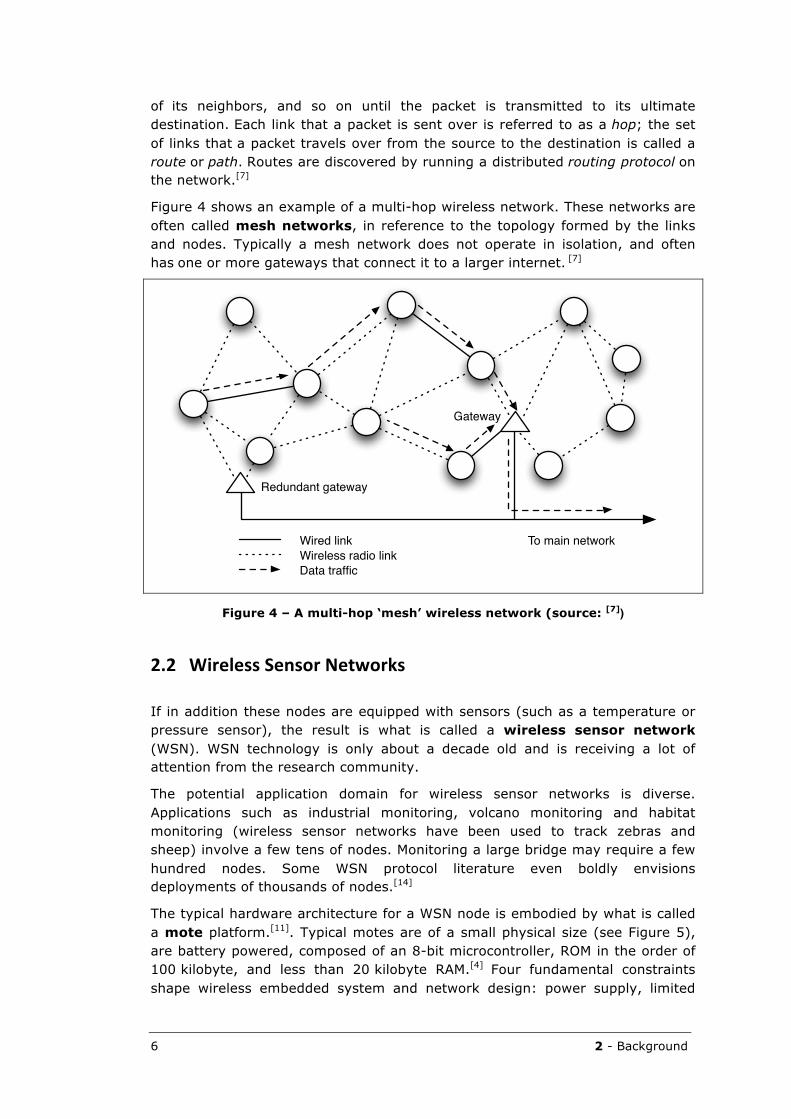
Figure 4 shows an example of a multi-hop wireless network. These networks are often called mesh networks, in reference to the topology formed by the links and nodes. Typically a mesh network does not operate in isolation, and often has one or more gateways that connect it to a larger internet. [7]
Figure 4 – A multi-hop ‘mesh’ wireless network (source: [7])
2.2 WirelessSensorNetworks
If in addition these nodes are equipped with sensors (such as a temperature or pressure sensor), the result is what is called a wireless sensor network (WSN). WSN technology is only about a decade old and is receiving a lot of attention from the research community.
The potential application domain for wireless sensor networks is diverse. Applications such as industrial monitoring, volcano monitoring and habitat monitoring (wireless sensor networks have been used to track zebras and sheep) involve a few tens of nodes. Monitoring a large bridge may require a few hundred nodes. Some WSN protocol literature even boldly envisions deployments of thousands of nodes.[14]
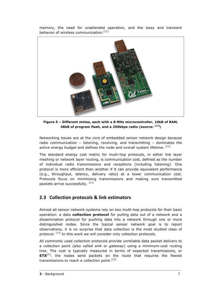
The typical hardware architecture for a WSN node is embodied by what is called a mote platform.[11]. Typical motes are of a small physical size (see Figure 5), are battery powered, composed of an 8-bit microcontroller, ROM in the order of 100 kilobyte, and less than 20 kilobyte RAM.[4] Four fundamental constraints shape wireless embedded system and network design: power supply, limited
Wired linkWireless radio linkData trafc
To main network
Redundant gateway
Gateway
2 - Background 7
memory, the need for unattended operation, and the lossy and transient behavior of wireless communication.[11]
Figure 5 – Different motes, each with a 8 MHz microcontroller, 10kB of RAM, 48kB of program flash, and a 250kbps radio (source: [11])
Networking issues are at the core of embedded sensor network design because radio communication – listening, receiving, and transmitting – dominates the active energy budget and defines the node and overall system lifetime. [11]
The standard energy cost metric for multi-hop protocols, in either link layer meshing or network layer routing, is communication cost, defined as the number of individual radio transmissions and receptions (including listening). One protocol is more efficient than another if it can provide equivalent performance (e.g., throughput, latency, delivery ratio) at a lower communication cost. Protocols focus on minimizing transmissions and making sure transmitted packets arrive successfully. [11]
2.3 Collectionprotocols&linkestimators
Almost all sensor network systems rely on two multi-hop protocols for their basic operation: a data collection protocol for pulling data out of a network and a dissemination protocol for pushing data into a network through one or more distinguished nodes. Since the typical sensor network goal is to report observations, it is no surprise that data collection is the most studied class of protocol. [11] In this work we will consider only collection protocols.
All commonly used collection protocols provide unreliable data packet delivery to a collection point (also called sink or gateway) using a minimum-cost routing tree. The cost is typically measured in terms of expected transmissions, or ETX[7]: the nodes send packets on the route that requires the fewest transmissions to reach a collection point.[11]
8 2 - Background
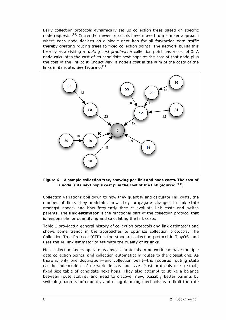
Early collection protocols dynamically set up collection trees based on specific node requests.[10] Currently, newer protocols have moved to a simpler approach where each node decides on a single next hop for all forwarded data traffic thereby creating routing trees to fixed collection points. The network builds this tree by establishing a routing cost gradient. A collection point has a cost of 0. A node calculates the cost of its candidate next hops as the cost of that node plus the cost of the link to it. Inductively, a node’s cost is the sum of the costs of the links in its route. See Figure 6.[11]
Figure 6 – A sample collection tree, showing per-link and node costs. The cost of a node is its next hop’s cost plus the cost of the link (source: [11])
Collection variations boil down to how they quantify and calculate link costs, the number of links they maintain, how they propagate changes in link state amongst nodes, and how frequently they re-evaluate link costs and switch parents. The link estimator is the functional part of the collection protocol that is responsible for quantifying and calculating the link costs.
Table 1 provides a general history of collection protocols and link estimators and shows some trends in the approaches to optimize collection protocols. The Collection Tree Protocol (CTP) is the standard collection protocol in TinyOS, and uses the 4B link estimator to estimate the quality of its links.
Most collection layers operate as anycast protocols. A network can have multiple data collection points, and collection automatically routes to the closest one. As there is only one destination—any collection point—the required routing state can be independent of network density and size. Most protocols use a small, fixed-size table of candidate next hops. They also attempt to strike a balance between route stability and need to discover new, possibly better parents by switching parents infrequently and using damping mechanisms to limit the rate
35
23
2222
36
2412
15
0
10
18
20
12
23
10 10
14
12
15
12
10
18
10
2 - Background 9
of change.[11]
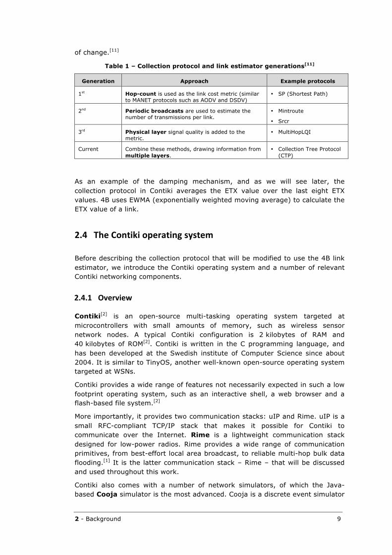
Table 1 – Collection protocol and link estimator generations[11]
Generation Approach Example protocols
1st Hop-count is used as the link cost metric (similar to MANET protocols such as AODV and DSDV)
• SP (Shortest Path)
2nd Periodic broadcasts are used to estimate the number of transmissions per link.
• Mintroute
• Srcr
3rd Physical layer signal quality is added to the metric.
• MultiHopLQI
Current Combine these methods, drawing information from multiple layers.
• Collection Tree Protocol (CTP)
As an example of the damping mechanism, and as we will see later, the collection protocol in Contiki averages the ETX value over the last eight ETX values. 4B uses EWMA (exponentially weighted moving average) to calculate the ETX value of a link.
2.4 TheContikioperatingsystem
Before describing the collection protocol that will be modified to use the 4B link estimator, we introduce the Contiki operating system and a number of relevant Contiki networking components.
2.4.1 Overview
Contiki[2] is an open-source multi-tasking operating system targeted at microcontrollers with small amounts of memory, such as wireless sensor network nodes. A typical Contiki configuration is 2 kilobytes of RAM and 40 kilobytes of ROM[2]. Contiki is written in the C programming language, and has been developed at the Swedish institute of Computer Science since about 2004. It is similar to TinyOS, another well-known open-source operating system targeted at WSNs.
Contiki provides a wide range of features not necessarily expected in such a low footprint operating system, such as an interactive shell, a web browser and a flash-based file system.[2]
More importantly, it provides two communication stacks: uIP and Rime. uIP is a small RFC-compliant TCP/IP stack that makes it possible for Contiki to communicate over the Internet. Rime is a lightweight communication stack designed for low-power radios. Rime provides a wide range of communication primitives, from best-effort local area broadcast, to reliable multi-hop bulk data flooding.[1] It is the latter communication stack – Rime – that will be discussed and used throughout this work.
Contiki also comes with a number of network simulators, of which the Java-based Cooja simulator is the most advanced. Cooja is a discrete event simulator
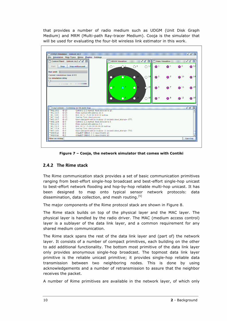
10 2 - Background
that provides a number of radio medium such as UDGM (Unit Disk Graph Medium) and MRM (Multi-path Ray-tracer Medium). Cooja is the simulator that will be used for evaluating the four-bit wireless link estimator in this work.
Figure 7 – Cooja, the network simulator that comes with Contiki
2.4.2 TheRimestack
The Rime communication stack provides a set of basic communication primitives ranging from best-effort single-hop broadcast and best-effort single-hop unicast to best-effort network flooding and hop-by-hop reliable multi-hop unicast. It has been designed to map onto typical sensor network protocols: data dissemination, data collection, and mesh routing.[5]
The major components of the Rime protocol stack are shown in Figure 8.
The Rime stack builds on top of the physical layer and the MAC layer. The physical layer is handled by the radio driver. The MAC (medium access control) layer is a sublayer of the data link layer, and a common requirement for any shared medium communication.
The Rime stack spans the rest of the data link layer and (part of) the network layer. It consists of a number of compact primitives, each building on the other to add additional functionality. The bottom most primitive of the data link layer only provides anonymous single-hop broadcast. The topmost data link layer primitive is the reliable unicast primitive; it provides single-hop reliable data transmission between two neighboring nodes. This is done by using acknowledgements and a number of retransmission to assure that the neighbor receives the packet.
A number of Rime primitives are available in the network layer, of which only
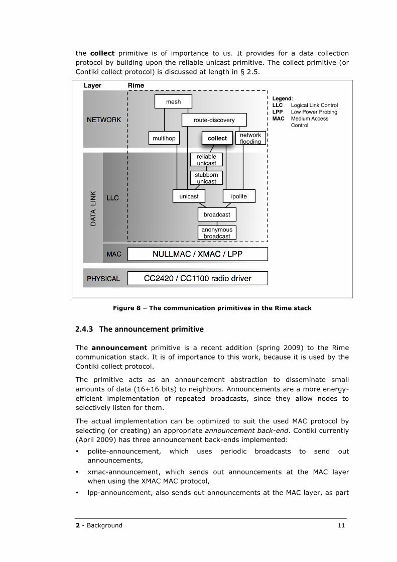
2 - Background 11
the collect primitive is of importance to us. It provides for a data collection protocol by building upon the reliable unicast primitive. The collect primitive (or Contiki collect protocol) is discussed at length in § 2.5.
Figure 8 – The communication primitives in the Rime stack
2.4.3 Theannouncementprimitive
The announcement primitive is a recent addition (spring 2009) to the Rime communication stack. It is of importance to this work, because it is used by the Contiki collect protocol.
The primitive acts as an announcement abstraction to disseminate small amounts of data (16+16 bits) to neighbors. Announcements are a more energy-efficient implementation of repeated broadcasts, since they allow nodes to selectively listen for them.
The actual implementation can be optimized to suit the used MAC protocol by selecting (or creating) an appropriate announcement back-end. Contiki currently (April 2009) has three announcement back-ends implemented:
• polite-announcement, which uses periodic broadcasts to send out announcements,
• xmac-announcement, which sends out announcements at the MAC layer when using the XMAC MAC protocol,
• lpp-announcement, also sends out announcements at the MAC layer, as part
PHYSICAL
MAC
NETWORK
NULLMAC / XMAC / LPP
CC2420 / CC1100 radio driver
RimeLayer
LLC
anonymous broadcast
broadcast
unicast
stubborn unicast
reliable unicast
collectmultihop
route-discovery
mesh
ipolite
network ooding
Legend:LLC Logical Link ControlLPP Low Power ProbingMAC Medium Access
Control
DATA
LIN
K
12 2 - Background
of the LPP beacons when using the Low Power Probing MAC protocol. [3]
The polite-announcement will be used when evaluating the Contiki collect protocol (see § 2.5). It is particularly suitable when using the Contiki nullmac MAC layer protocol in the Cooja simulator. The nullmac MAC layer protocol is a simple pass-through protocol, and doesn’t perform any medium access control.
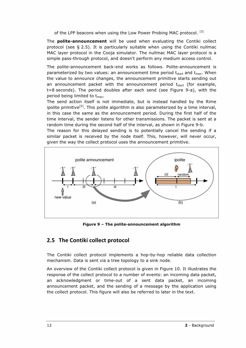
The polite-announcement back-end works as follows. Polite-announcement is parameterized by two values: an announcement time period tstart and tmax. When the value to announce changes, the announcement primitive starts sending out an announcement packet with the announcement period tstart (for example, t=8 seconds). The period doubles after each send (see Figure 9-a), with the period being limited to tmax. The send action itself is not immediate, but is instead handled by the Rime ipolite primitive[5]. This polite algorithm is also parameterized by a time interval, in this case the same as the announcement period. During the first half of the time interval, the sender listens for other transmissions. The packet is sent at a random time during the second half of the interval, as shown in Figure 9-b. The reason for this delayed sending is to potentially cancel the sending if a similar packet is received by the node itself. This, however, will never occur, given the way the collect protocol uses the announcement primitive.
Figure 9 – The polite-announcement algorithm
2.5 TheContikicollectprotocol
The Contiki collect protocol implements a hop-by-hop reliable data collection mechanism. Data is sent via a tree topology to a sink node.
An overview of the Contiki collect protocol is given in Figure 10. It illustrates the response of the collect protocol to a number of events: an incoming data packet, an acknowledgment or time-out of a sent data packet, an incoming announcement packet, and the sending of a message by the application using the collect protocol. This figure will also be referred to later in the text.
t 2t 4t
new value
t
polite announcement ipolite
t/2 random
(a) (b)
2 - Background 13
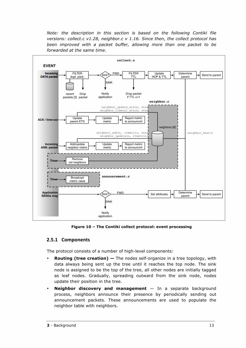
Note: the description in this section is based on the following Contiki file versions: collect.c v1.28, neighbor.c v 1.16. Since then, the collect protocol has been improved with a packet buffer, allowing more than one packet to be forwarded at the same time.
Figure 10 – The Contiki collect protocol: event processing
2.5.1 Components
The protocol consists of a number of high-level components:
• Routing (tree creation) — The nodes self-organize in a tree topology, with data always being sent up the tree until it reaches the top node. The sink node is assigned to be the top of the tree, all other nodes are initially tagged as leaf nodes. Gradually, spreading outward from the sink node, nodes update their position in the tree.
• Neighbor discovery and management — In a separate background process, neighbors announce their presence by periodically sending out announcement packets. These announcements are used to populate the neighbor table with neighbors.
FILTERdupl. pack.
FILTERTTL
UpdateHOP & TTL
Determine parent Send to parentIncoming
DATA packet Sink?
Update parent ETX
Update metric
Report metric to announcmt
Add/update neighbor metric
Update metric
Report metric to announcmt
ACK / time-out
Incoming ANN. packet
Removeold neighborsTimer
Timer
Application SENDs msg
Broadcast metric value
Sink? Set attributes Determine parent Send to parent
recentpackets [2]
neighbors [8]
Drop packet
Notifyapplication
Drop packetif TTL <=1
SINK
FWD
EVENT
neighbor.c
announcement.c
neighbor_update_etx(n, etx)neighbor_timeout_etx(n, etx)
neighbor_add(n, rtmetric, etx)neighbor_update(n, rtmetric)
neighbor_best()
Notifyapplication
SINK
FWD
collect.c
14 2 - Background
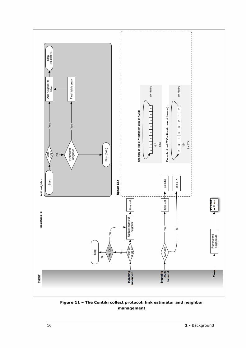
• Link estimation — Based on link level acknowledgments for data packets sent by the node, the ETX value of each neighbor in the neighbor table is updated on each acknowledgment or time-out.
• Duplicate packet filtering and packet aging — Packets get forwarded by nodes until they reach the sink node. To protect against forwarding duplicate packets, a node checks a packet to be forwarded against a limited history of forwarded packets. If it has recently been forwarded, the packet is dropped. Additionally, to prevent packets from roaming through the network forever, the packet is dropped if it exceeds a certain maximum number hops.
On a side note, the Contiki collect protocol does not contain any loop detection mechanism. Routing loops generally occur when a node chooses a new route that has a significantly higher ETX than its old one, perhaps in response to losing connectivity with a candidate parent. If the new route includes a node which was a descendant, then a loop occurs.[18] It would be interesting to investigate and implement a number of practical solutions to alleviate this. For example, the collect protocol could be modified to include the current node’s routing cost gradient in the packet header, and prevent the receiving node from forwarding packets with a lower gradient. [18]
2.5.1.1 Routing(treecreation)
The routing mechanism to transport data originating from any node to the sink node builds a routing tree (see also § 2.3).
All nodes are organized in a virtual tree, with their position in the tree defined by a 16-bit rtmetric (route metric) value. The sink node, at the top of the tree, has an rtmetric value 0. Child nodes further down the tree have an increasing rtmetric value. The parent of a node is the best neighbor of node, i.e. the node that minimizes the expected number of transmission to the sink.
The tree is created dynamically by updating the rtmetric value at particular events. Initially all nodes have the maximum rtmetric value (this maximum is currently set to 255, not all 16 bits are used), except for the sink node which has value 0 assigned by the application using the collect protocol. The announcement packets sent out for neighbor discovery (see § 2.5.1.1) report the rtmetric value of the announcing node. This neighbor's rtmetric value is stored in the neighbor table of each receiving node.
The node's own rtmetric value is then calculated based on the rtmetric value of the best neighbor node. The best neighbor node is the node that provides the path with the fewest expected transmissions to the sink node. This is the case for the neighbor that minimizes the sum of the neighbor rtmetric and the expected number of transmissions (ETX) from the node to that neighbor.
€
rtmetric = argminn∈N
(rtmetricn + ETXn ) (eq. 1)
The rtmetric value is updated on the following events: designation of a node as sink node, an incoming announcement packet, the acknowledgement of a data packet and the time-out of a data packet.
The rtmetric calculation process gradually trickles down from the neighbors of
2 - Background 15
the sink node to the leaf nodes. Once the process has stabilized, the rtmetric of a node represents the expected number of total transmission for a packet to arrive at the sink node.
2.5.1.2 Neighbordiscoveryandmanagement
See Figure 11.
Neighbor discovery and management is located in a separate code module (core/net/rime/neighbor.c). This is also the location where the neighbor table is managed.
Neighbor discovery is organized using the Rime announcement primitive, see § 2.4.3. The announcement primitive periodically sends out announcement packets (specifically tagged as such) on a separate logical channel. Announcements are characterized by an (ID, value) tuple and are disseminated to local area neighbors. Incoming announcement packets do not traverse the complete Rime stack, but instead are intercepted at the MAC layer. The MAC layer then notifies any registered processes (based on the announcement ID) about the incoming announcement.
The collect protocol is such a registered process, and it uses the incoming announcement to populate a neighbor table. The announcement specifies the sending neighbor address, the ID (which is set to the channel number but of no further use), while the value represents the routing metric used for tree creation and routing. Since the neighbor table is limited in size (currently set to 8 neighbors), it is important that 'old' neighbors do not occupy the table for too long. Thereto, a timer triggers periodic (i.e., every second) scanning of the neighbor table and removes all neighbors which haven't been heard from during the previous 120 scans (i.e., roughly 120 seconds).
2.5.1.3 Linkestimation
See Figure 11.
The ETX values for each node's neighbors are stored in the neighbor table, and are calculated each time a data packet is sent to a neighbor. When the sent packed is ACK'ed, the number of transmissions that was required to deliver the packet is reported to the link estimator.
Each of the last eight transmission counts is kept in the table. The link ETX value from a node to a neighbor is then the average over these eight transmission counts. If a transmission times out, the maximum number of transmission (e.g., 4) is reported and added to the current history entry (instead of overwriting it).
16 2 - Background
Figure 11 – The Contiki collect protocol: link estimator and neighbor management
!"!#$ $%&'(
!"#$%&'(&%)*+',-'
.&*/01,)
2&*/01,)'
*.'%$13&4
2,
5##'674
8&9
:&(,;&',3#'
.&*/01,<)9
=%,"
%*(&'>'?
-,)'&$+0'
.@'%*(&AA
-,)'&$+0'
.@'%*(&A
A
2, 5B7
)*+,&%*-.
/012
3%&'4,53
%*(&'>'?
8&9!"#$%&'()*
=&&'C*/<)&'DD
)*+,&%*-.
6**,5*+&7
2,
89:63'.!$;
=&&'C*/<)&'DDD
/::.*'%-<=,(
9&%'EFD
$##'EFD
GH
IJ
HG
IK
GH
IJ
HG
IK
EFD
H'A'EFD
&%L'0*9%,)M
&%L'0*9%,)M
!>6&9?'.,@.AB'3.!$;A.6+3%,*.C%*.+6B'.,@.3%&'4,53DE
!>6&9?'.,@.AB'3.!$;A.6+3%,*.C%*.+6B'.,@./01DE
89:63'.!$;
N&('
$;$*34
C3<90'%$13&'&.%)M
5##'.&*/01,)'%,'
%$13&
8&9
2,
=%,"'OC5PQR
C*.#'S,)9%'
.&*/01,)
8&9
=%,"'
O=!BBE=R
=%$)%
2 - Background 17
2.5.1.4 Duplicatepacketfilteringandpacketaging
See also Figure 10.
Duplicate packets can be created upon retransmission when the ACK is lost. Without duplicate packet elimination, these will be forwarded, possibly causing more retransmissions and more contention, and wasting energy. To protect against forwarding duplicate packets, a node will not forward a packet that it has recently forwarded. Thereto it keeps a small history of recently forwarded packets (currently 2 packets), which are uniquely characterized by their packet ID (EPACKET_ID) and originating node (ESENDER). If a node receives a packet that has the same ID and originator address, the packet is dropped.
Additionally, to prevent packets from roaming through the network forever, the packet is dropped if it exceeds a certain maximum number hops. Thereto each packet has a time-to-live (TTL) attribute, which is initialized to 10 and gets decremented each time a packet is forwarded. On receiving a packet with a TTL value of 1 or lower, the node drops the packet.
2.5.2 Protocolattributes
The following attributes (i.e. fields) are attached to a packet sent using the collect protocol:
• EPACKET_ID. Each packet originating from a node gets a 4-bit packet ID (also called sequence number). Together with the originating address stored in the ESENDER attribute, it uniquely identifies the packet.
• ESENDER. The address of the node initializing the send of the packet.
• HOPS. This attribute represents the current hop count. It is initialized to 1, and will be incremented on each forward by a node.
• TTL. The time-to-live represent the maximum number of hops the packet can make. It is initialized to 10. On each forward by a node, the TTL value is decreased by 1. If a node receives a packet with TTL equal to (or lower than) 1, the packet is discarded. This prevents packets from traveling through the network forever.
• MAX_REXMIT. Used by the underlying reliable unicast Rime layer (runicast). This value represents the maximum number of link-level transmissions to send or forward the packet to a neighbor. If the maximum number of transmissions is reached, the packet times out. Upon time-out of a packet, the packet is dropped, the neighbor ETX data is updated, and the rtmetric is updated as well.
Note that there is no destination address attribute, since for the collect protocol all data is send to the sink, i.e. the node with the routing metric 0.
The following table lists the attributes attached to a packet by the collect protocol and underlying Rime layers (shown from left to right).
18 2 - Background
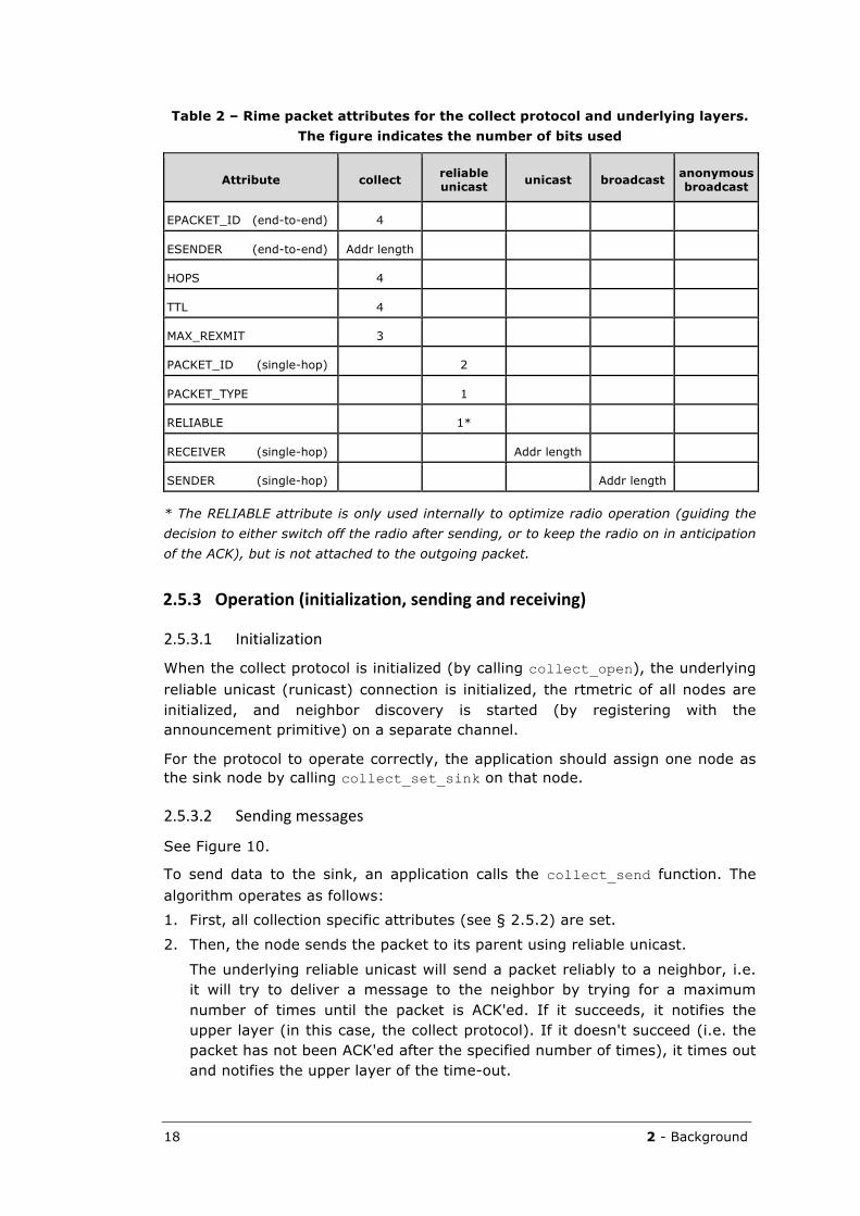
Table 2 – Rime packet attributes for the collect protocol and underlying layers. The figure indicates the number of bits used
Attribute collect reliable unicast unicast broadcast anonymous
broadcast
EPACKET_ID (end-to-end) 4
ESENDER (end-to-end) Addr length
HOPS 4
TTL 4
MAX_REXMIT 3
PACKET_ID (single-hop) 2
PACKET_TYPE 1
RELIABLE 1*
RECEIVER (single-hop) Addr length
SENDER (single-hop) Addr length
* The RELIABLE attribute is only used internally to optimize radio operation (guiding the decision to either switch off the radio after sending, or to keep the radio on in anticipation of the ACK), but is not attached to the outgoing packet.
2.5.3 Operation(initialization,sendingandreceiving)
2.5.3.1 Initialization
When the collect protocol is initialized (by calling collect_open), the underlying
reliable unicast (runicast) connection is initialized, the rtmetric of all nodes are initialized, and neighbor discovery is started (by registering with the announcement primitive) on a separate channel.
For the protocol to operate correctly, the application should assign one node as the sink node by calling collect_set_sink on that node.
2.5.3.2 Sendingmessages
See Figure 10.
To send data to the sink, an application calls the collect_send function. The
algorithm operates as follows:
1. First, all collection specific attributes (see § 2.5.2) are set.
2. Then, the node sends the packet to its parent using reliable unicast.
The underlying reliable unicast will send a packet reliably to a neighbor, i.e. it will try to deliver a message to the neighbor by trying for a maximum number of times until the packet is ACK'ed. If it succeeds, it notifies the upper layer (in this case, the collect protocol). If it doesn't succeed (i.e. the packet has not been ACK'ed after the specified number of times), it times out and notifies the upper layer of the time-out.
2 - Background 19
The parent node is determined each time upon sending by requesting the best neighbor from the neighbor table. If no best neighbor can be found (i.e., the table is empty), the packet is dropped and the node actively listens for announcements (during a limited period) to detect potential neighbors.
Should the send function have been called on the node that is the sink node, the receive function of the application using the collect protocol is called, and no reliable unicast send takes place.
3. When the sent packet gets ACK'ed by the parent (node_packet_sent is called) or times out (node_packet_timedout is called), the node's rtmetric and the ETX of the parent is updated.
2.5.3.3 Receivingmessages
See Figure 10.
Two types of packets can be received: data packets and announcement packets.
Data packets
When a node receives a collection data packet (via reliable unicast which calls the function node_packet_received) several things happen:
• First, duplicate packet filtering is executed: the packet is checked against the last two forwarded packets. If the ID (EPACKET_ID attribute) and originator address (ESENDER attribute) match with any of these, the packet is dropped. If not dropped, the ID and originator address of the received packet is stored in the recently forwarded packets table.
• If the node receiving the packet is the sink node, the application using the collect protocol is notified of the reception of a packet. The originator address, packet ID and number of hops the packet has travelled are provided as arguments.
• If the node receiving the packet is NOT the sink node, the packet has to be forwarded.
• If the TTL value is 1 (or lower), the packet is dropped.
• The HOP count is incremented, and the TTL is decremented.
• The packet is forwarded to its parent using the underlying reliable unicast layer. The parent selection is identical as described under "Sending messages" (see § 2.5.3.2).
When a packet has not yet been ACK'ed or timed-out, new packets cannot be forwarded but are dropped instead. In a recent update of the collect protocol, a packet queue has been added. This will not be considered in this work however.
Announcement packets
When a node receives an announcement packet (received_announcement is
called by the announcement back-end, see § 2.4.3) the following actions are taken:
• The neighbor who sent out the announcement is checked against the neighbor table. If not yet present, the neighbor is added to the table.
20 2 - Background
Otherwise, the neighbor's rtmetric value is updated in the neighbor table.
If the neighbor table is full, the worst neighbor in the neighbor table is evicted, and replaced by the new neighbor (see Figure 11). The worst neighbor is defined as the neighbor with the highest route metric to the sink.
• The node updates its rtmetric.
2.6 Thefour‐bitwirelesslinkestimator(4B)
The link estimator in the Contiki collect protocol bases its calculation on information from the data link layer only, i.e. link level acknowledgments or time-outs.
The four-bit wireless link estimator (4B), proposed by Fonseca et al. [8], provides well-defined interfaces to combine information from the physical, data-link and network layers for link estimation. 4B uses ETX (see § 2.3) as the link quality metric.
In 4B, the interfaces provide 4 bits of information compiled from different layers:
• A white bit from the physical layer, denoting the low probability of decoding error in received packets. If the white bit is set, the medium quality is high. If the white bit is not set, then the medium quality may or may not have been high during the packet’s reception. As a rule of thumb, the medium quality is considered high when the Link Quality Indication (LQI) of a packet is above 90%. The LQI is a characterization of the strength and/or quality of a received packet, as defined by the IEEE 802.15.4 Standard.[12]
• An ack bit from the data link layer, indicating if an acknowledgment is received for a sent packet. If the bit is set, the packet was acknowledged by the data link layer transmission. If not set, the packet may or may not have been received successfully.
• A pin bit from the network layer, indicating if the link estimator can remove the neighbor entry from its neighbor table or not. The network layer sets the pin bit for those entries that should not be removed from the table. This makes sense for, for example, the neighbors of the sink node: they would want to keep the sink in their neighbor table at all cost.
• A compare bit from the network layer, indicating if the metric value of the neighbor from which a packet was received is better – i.e. lower – than the metric value of one or more entries in the neighbor table. If the bit is set, the network signals that the path through that neighbor is better than a path through at least one neighbor in the neighbor table.
Figure 12 shows 4B mapped to the Rime protocol stack. 4B is typically represented by a triangle to indicate the three layers that it utilizes.
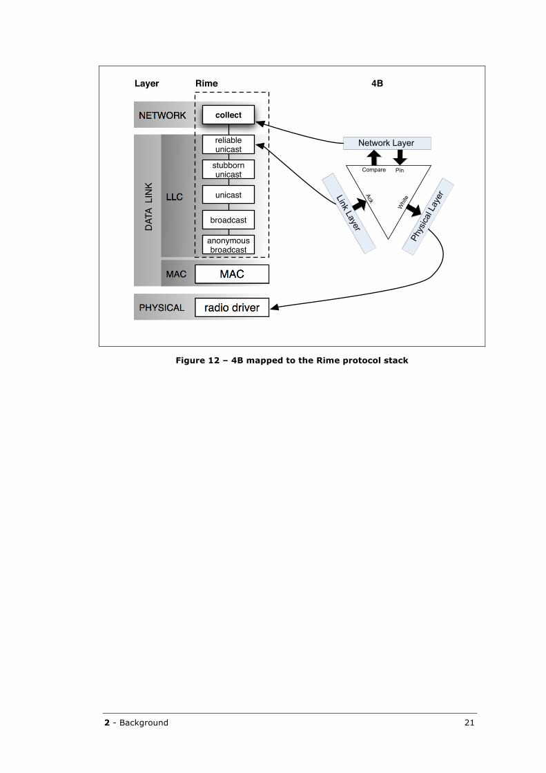
2 - Background 21
Figure 12 – 4B mapped to the Rime protocol stack
PHYSICAL
MAC
NETWORK
MAC
radio driver
RimeLayer
LLC
anonymous broadcast
broadcast
unicast
stubborn unicast
reliable unicast
collect
4B
DATA
LIN
K

22 2 - Background
3 - Implementation of 4B 23
3 Implementationof4B
In this section we will look at the operation details of the 4B estimator, show how it is different from the collect estimator, and discuss some Contiki implementation notes. A modified reliable unicast Rime primitive will also be introduced to correct for a flaw in the current reliable unicast Rime primitive.
3.1 Wheredoes4Bfitin?
As outlined in § 2.5.1, the Contiki collect protocol is made up of a number of high level components: neighbor discovery & management, link estimation and routing.
The implementation of 4B will impact the first two components (neighbor discovery & management and link estimation). The routing component will be kept identical for the 4B implementation.
3.2 The4Bhybridestimatoralgorithm
The 4B link estimator that will be implemented in the Contiki collect protocol is based on the 4B TinyOS implementation (see [17], [18] and [19]).
The 4B link estimator described in the 4B paper[8] and also implemented in TinyOS is a hybrid link estimator: to calculate the link quality it combines the information provided by the three layers with periodic beacons (i.e. broadcast packets without any payload).
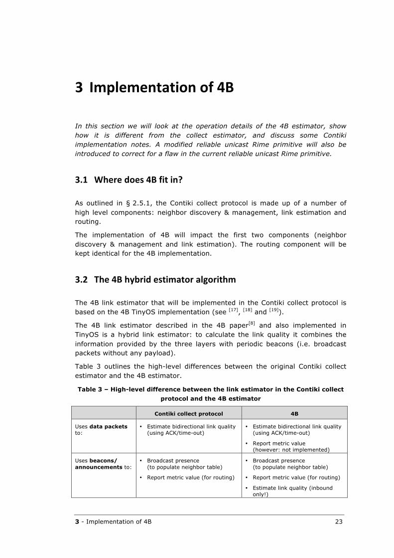
Table 3 outlines the high-level differences between the original Contiki collect estimator and the 4B estimator.
Table 3 – High-level difference between the link estimator in the Contiki collect protocol and the 4B estimator
Contiki collect protocol 4B
Uses data packets to:
• Estimate bidirectional link quality (using ACK/time-out)
• Estimate bidirectional link quality (using ACK/time-out)
• Report metric value (however: not implemented)
Uses beacons/ announcements to:
• Broadcast presence (to populate neighbor table)
• Report metric value (for routing)
• Broadcast presence (to populate neighbor table)
• Report metric value (for routing)
• Estimate link quality (inbound only!)

24 3 - Implementation of 4B
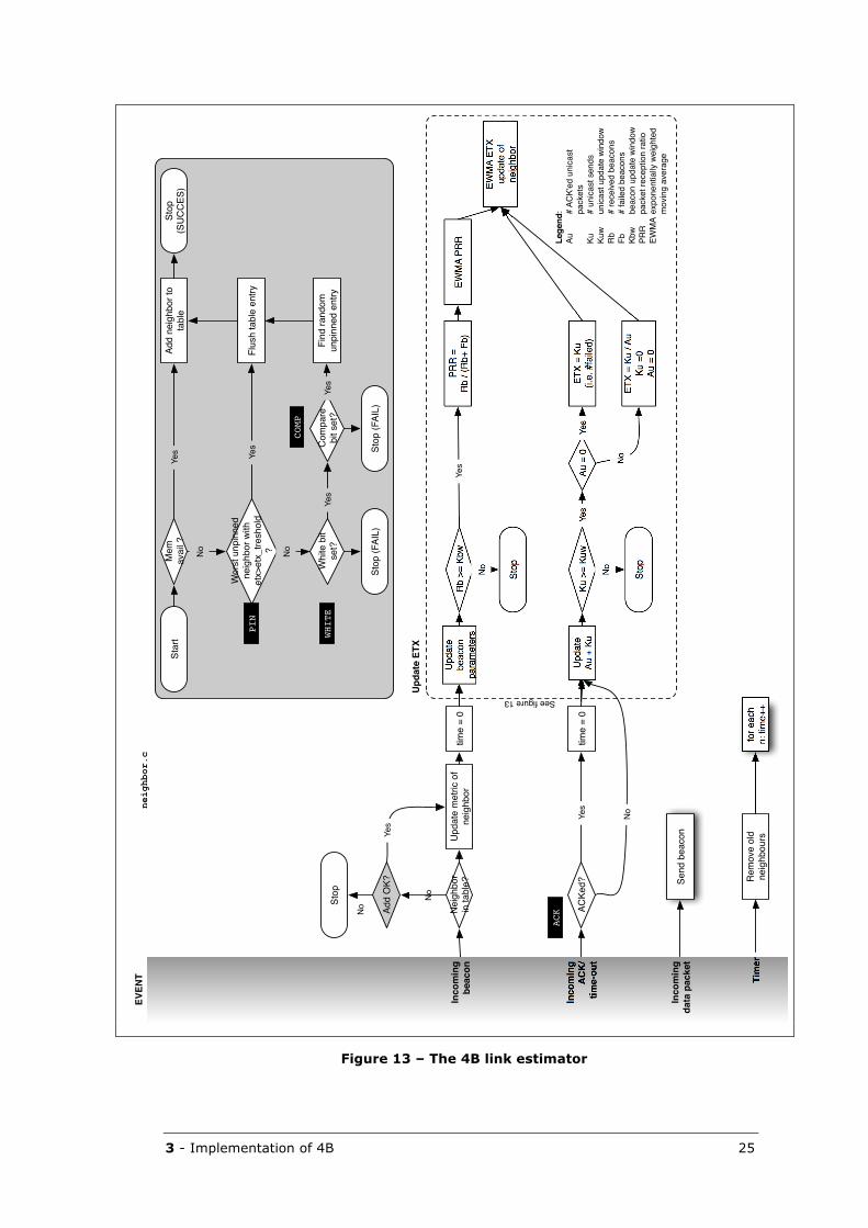
Figure 13 shows where each of the four bits is used in the 4B algorithm. The ack bit is used for sent data packets to calculate the ETX value. The pin, white and compare bit are all used to decide upon insertion of a neighbor in the neighbor table.
As can be seen when comparing Figure 11 with Figure 13 the differences between the Contiki collect protocol estimator and the 4B estimator are:
• a different neighbor eviction/insertion policy,
• usage of data packets, in addition to beacons, to update link quality,
• a different link quality (i.e. ETX) calculation.
3 - Implementation of 4B 25
Figure 13 – The 4B link estimator
!"!#$ $%&'(
!"#$%&'(&%)*+',-'
.&*/01,)
2&*/01,)'
*.'%$13&4
2,
5##'674
8&9
:&(,;&',3#'
.&*/01,<)9
=%,"
%*(&'>'?
-,)'&$+0'
.@'%*(&AA
-,)'&$+0'
.@'%*(&AA
2, 5B7
)*+,&%*-.
/012
3%&'4,53
%*(&'>'?
8&9!"#$%&'()*
!"#$%&'
5<'A'7<
7<'C>'7<D
5<'>'?
EFG'>'7<'
H*I&I'J-$*3&#K
EFG'>'7<'L'5<
7<'>?
5<'>'?
EMN5'EFG'
<"#$%&',-'
.&*/01,)
!"#$%&'
1&$+,.'
"$)$(&%&)9
:1'C>'71D
EMN5'O::
O::'>'
:1'L'H:1A'P1K
=%,"
=%,"
8&9
2,
2,
8&9
67893'.!$:
2,
8&9
;'-'*8@
5<
J'5B7Q&#'<.*+$9%
"$+R&%9
7<
J'<.*+$9%'9&.#9
7<D
<.*+$9%'<"#$%&'D*.#,D
:1
J')&+&*;&#'1&$+,.9
P1
J'-$*3&#'1&$+,.9
71D
1&$+,.'<"#$%&'D*.#,D
O::
"$+R&%')&+&"%*,.')$%*,
EMN5&S",.&.%*$33T'D&*/0%&#
(,;*./'$;&)$/&
=&&'!/<)&'UV
=&.#'1&$+,.
)*+,&%*-.
8939.79+<'3
2,
)*+,&%*-.
='9+,*
M0*%&'1*%'
9&%4
B,("$)&'
1*%'9&%4
N&('
$;$*3'4
P*.#')$.#,('
<."*..&#'&.%)T
P3<90'%$13&'&.%)T
5##'.&*/01,)'%,'
%$13&
8&9
2,
=%,"'HP5WXK
=%,"'HP5WXK
M,)9%'<."*..&#'
.&*/01,)'D*%0'
&%SC&%SY%)&90,3#
4
8&9
2,
8&9
=%,"'
H=!BBE=K
=%$)%
!"#$
%&'()
$'*
8&9
+!,
26 3 - Implementation of 4B
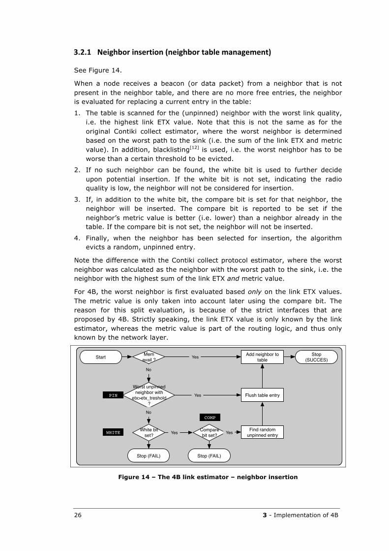
3.2.1 Neighborinsertion(neighbortablemanagement)
See Figure 14.
When a node receives a beacon (or data packet) from a neighbor that is not present in the neighbor table, and there are no more free entries, the neighbor is evaluated for replacing a current entry in the table:
1. The table is scanned for the (unpinned) neighbor with the worst link quality, i.e. the highest link ETX value. Note that this is not the same as for the original Contiki collect estimator, where the worst neighbor is determined based on the worst path to the sink (i.e. the sum of the link ETX and metric value). In addition, blacklisting[12] is used, i.e. the worst neighbor has to be worse than a certain threshold to be evicted.
2. If no such neighbor can be found, the white bit is used to further decide upon potential insertion. If the white bit is not set, indicating the radio quality is low, the neighbor will not be considered for insertion.
3. If, in addition to the white bit, the compare bit is set for that neighbor, the neighbor will be inserted. The compare bit is reported to be set if the neighbor’s metric value is better (i.e. lower) than a neighbor already in the table. If the compare bit is not set, the neighbor will not be inserted.
4. Finally, when the neighbor has been selected for insertion, the algorithm evicts a random, unpinned entry.
Note the difference with the Contiki collect protocol estimator, where the worst neighbor was calculated as the neighbor with the worst path to the sink, i.e. the neighbor with the highest sum of the link ETX and metric value.
For 4B, the worst neighbor is first evaluated based only on the link ETX values. The metric value is only taken into account later using the compare bit. The reason for this split evaluation, is because of the strict interfaces that are proposed by 4B. Strictly speaking, the link ETX value is only known by the link estimator, whereas the metric value is part of the routing logic, and thus only known by the network layer.
Figure 14 – The 4B link estimator – neighbor insertion
Mem avail?
Flush table entry
Add neighbor to tableYes
No
Stop (FAIL)
Find worst neighbor Yes
Stop (SUCCES)Start
White bit set?
Compare bit set?
Mem avail ?
Find random unpinned entry
Flush table entry
Add neighbor to table
Yes
No
Stop (FAIL) Stop (FAIL)
Worst unpinned neighbor with
etx>etx_treshold?
Yes
No
Yes
Stop (SUCCES)Start
COMP
WHITE
PIN
Yes
3 - Implementation of 4B 27
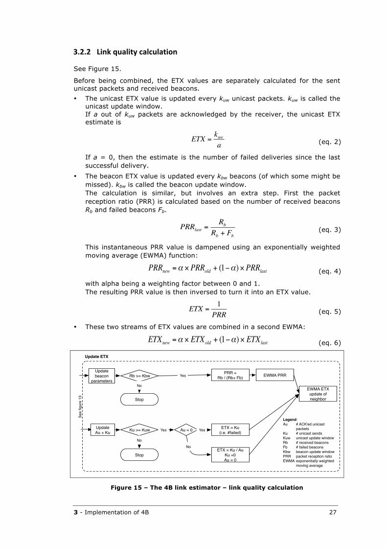
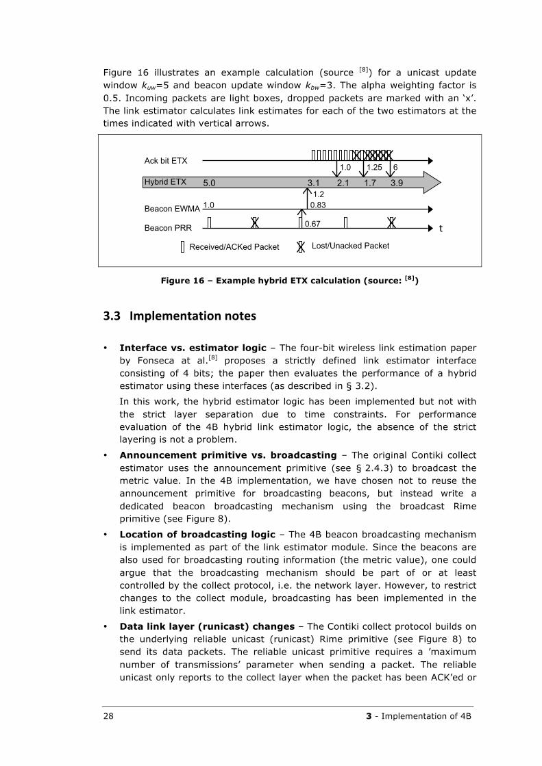
3.2.2 Linkqualitycalculation
See Figure 15.
Before being combined, the ETX values are separately calculated for the sent unicast packets and received beacons.
• The unicast ETX value is updated every kuw unicast packets. kuw is called the unicast update window. If a out of kuw packets are acknowledged by the receiver, the unicast ETX estimate is
€
ETX =kuwa (eq. 2)
If a = 0, then the estimate is the number of failed deliveries since the last successful delivery.
• The beacon ETX value is updated every kbw beacons (of which some might be missed). kbw is called the beacon update window. The calculation is similar, but involves an extra step. First the packet reception ratio (PRR) is calculated based on the number of received beacons Rb and failed beacons Fb.
€
PRRlast =Rb
Rb + Fb (eq. 3)
This instantaneous PRR value is dampened using an exponentially weighted moving average (EWMA) function:
€
PRRnew =α × PRRold + (1−α) × PRRlast (eq. 4)
with alpha being a weighting factor between 0 and 1. The resulting PRR value is then inversed to turn it into an ETX value.
€
ETX =1
PRR (eq. 5)
• These two streams of ETX values are combined in a second EWMA:
€
ETXnew =α × ETXold + (1−α) × ETXlast (eq. 6)
Figure 15 – The 4B link estimator – link quality calculation
Update Au + Ku Ku >= Kuw Au = 0 ETX = Ku
(i.e. #failed)
ETX = Ku / AuKu =0Au = 0
EWMA ETX update of neighbor
Update beacon
parametersRb >= Kbw EWMA PRRPRR =
Rb / (Rb+ Fb)
Stop
Stop
Yes
No
No
Yes
Update ETX
No
Yes
Legend:Au # ACK'ed unicast
packetsKu # unicast sendsKuw unicast update windowRb # received beaconsFb # failed beaconsKbw beacon update windowPRR packet reception ratioEWMA exponentially weighted
moving average
See g
ure
13
28 3 - Implementation of 4B
Figure 16 illustrates an example calculation (source [8]) for a unicast update window kuw=5 and beacon update window kbw=3. The alpha weighting factor is 0.5. Incoming packets are light boxes, dropped packets are marked with an ‘x’. The link estimator calculates link estimates for each of the two estimators at the times indicated with vertical arrows.
Figure 16 – Example hybrid ETX calculation (source: [8])
3.3 Implementationnotes
• Interface vs. estimator logic – The four-bit wireless link estimation paper by Fonseca at al.[8] proposes a strictly defined link estimator interface consisting of 4 bits; the paper then evaluates the performance of a hybrid estimator using these interfaces (as described in § 3.2).
In this work, the hybrid estimator logic has been implemented but not with the strict layer separation due to time constraints. For performance evaluation of the 4B hybrid link estimator logic, the absence of the strict layering is not a problem.
• Announcement primitive vs. broadcasting – The original Contiki collect estimator uses the announcement primitive (see § 2.4.3) to broadcast the metric value. In the 4B implementation, we have chosen not to reuse the announcement primitive for broadcasting beacons, but instead write a dedicated beacon broadcasting mechanism using the broadcast Rime primitive (see Figure 8).
• Location of broadcasting logic – The 4B beacon broadcasting mechanism is implemented as part of the link estimator module. Since the beacons are also used for broadcasting routing information (the metric value), one could argue that the broadcasting mechanism should be part of or at least controlled by the collect protocol, i.e. the network layer. However, to restrict changes to the collect module, broadcasting has been implemented in the link estimator.
• Data link layer (runicast) changes – The Contiki collect protocol builds on the underlying reliable unicast (runicast) Rime primitive (see Figure 8) to send its data packets. The reliable unicast primitive requires a ’maximum number of transmissions’ parameter when sending a packet. The reliable unicast only reports to the collect layer when the packet has been ACK’ed or
1.0
1.0 0.83
5.0 3.1 1.72.1
1.25 6
3.9
0.67
1.2
Ack bit ETX
Received/ACKed Packet Lost/Unacked Packet
Hybrid ETX
Beacon EWMA
Beacon PRR t
3 - Implementation of 4B 29
when the maximum number of transmission has been reached (i.e. a time-out). The 4B estimator, however, requires reporting of an acknowledgment or absence thereof after each packet (re)sent. Thereto, the reliable unicast primitive had to be changed to support notifying the link estimator upon each individual ACK or time-out.
• ETX vs. EETX – The 4B TinyOS implementation internally represents the link quality as extra expected number of transmissions (EETX). So, an optimal link has a link quality of EETX=0, corresponding to one transmission (ETX=1). In the 4B Contiki implementation regular ETX values have been used instead of EETX values.
• WHITE BIT (LQI) – For the CC2420 radio, present in the Sentilla Jcreate motes used at VUB, the white bit is set when the Link Quality Indication (LQI) of a packet is above 105. The LQI is a characterization of the strength and/or quality of a received packet, as defined by the IEEE 802.15.4 Standard.[12] The LQI value range is specified[12] to be from 0 – 225. However, the range of LQI returned by the CC2420 radio is from 50 to 110[16]. So a packet with an LQI value greater than 105 indicates a link quality better than 90%. In Contiki, the LQI can be queried directly through a sensor interface call.
• PIN BIT – In the 4B TinyOS implementation, a neighbor is pinned in two cases: (a) if the neighbor is the sink node, or (b) if the neighbor is elected as parent (when a new parent is chosen, the old parent is unpinned). This prevents the parent or sink from being removed from the neighbor table (see Figure 14). In the 4B Contiki implementation, the pin bit logic is not explicitly implemented (i.e. no arbitrary neighbors can be pinned by the collect protocol). However, the parent neighbor is prevented from being evicted.
3.4 RewriteoftheRimereliableunicastprimitive
3.4.1 Theproblem
As mentioned in § 3.3, the Contiki collect protocol uses reliable unicast (runicast) to send its packet to a single-hop neighbor (see also § 2.4.2).
It turned out that the default runicast implementation is inherently flawed in reporting the number of required transmissions to the upper layer primitive (collect, in our case). This value is critical however to correctly evaluate the performance of both link estimators. Therefore, reliable unicast had to be rewritten to support correct (re)transmission count reporting.
The reason for the flaw is the way in which runicast builds on stubborn unicast (stunicast) to deliver its packets reliably (see Figure 17).
The stunicast primitive sends and resends the packet until the upper layer primitive (runicast) cancels the transmission. Stunicast reports to runicast each
30 3 - Implementation of 4B
time it has (re)sent the packet. Based on this reporting, runicast will let stunicast continue sending, or, if the maximum number of transmissions has been reached, will instruct stunicast to cancel the repeated sending and report a time-out to the upper layer primitive (e.g. collect).
This interaction is flawed, and makes it for example possible for runicast to both report a time-out and an acknowledgment to the upper layer primitive. This is easy to illustrate if we consider a packet that has to be sent reliable with a maximum transmission count of 1:
1. Runicast will instruct stunicast to start sending the packet.
2. Stunicast will send the packet, schedule the next resend, and report the send to runicast.
3. Since runicast keeps track of the maximum number of transmissions (i.e. 1), and since this value has now been reached, it will instruct stunicast to cancel any subsequent sends. Runicast will report a time-out to the upper layer primitive (collect) because the maximum number of transmissions has been reached.
4. However, the packet that was sent might by now be ACK’ed. So, runicast will now also report an ACK to the upper layer primitive, while it has already reported a time-out!
The reason for this bug is that the reporting from stunicast to runicast about the sent packet is too late. Stunicast should report to runicast just before resending, so that runicast can cancel the pending resent in case the maximum transmission count has been reached.
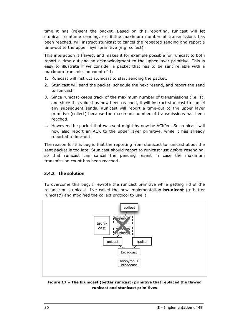
3.4.2 Thesolution
To overcome this bug, I rewrote the runicast primitive while getting rid of the reliance on stunicast. I’ve called the new implementation brunicast (a ‘better runicast’) and modified the collect protocol to use it.
Figure 17 – The brunicast (better runicast) primitive that replaced the flawed runicast and stunicast primitives
anonymous broadcast
broadcast
unicast
stubborn unicast
reliable unicast
collect
ipolite
bruni-cast
3 - Implementation of 4B 31
The brunicast primitive schedules an evaluation instead of a resend. If an acknowledgment packet is received before the evaluation function has been called, the scheduled evaluation is canceled, and the acknowledgment is reported to the upper layer primitive. If no acknowledgment comes in, the evaluation function is called when the timer expires. Upon evaluation, the packet is either resend if the maximum transmission count has not yet been reached, or a time-out is reported to the upper layer primitive in the other case.
I’ve submitted brunicast to replace runicast and stunicast in the official source tree.

32 3 - Implementation of 4B
4 - Evaluation of 4B 33
4 Evaluationof4B
In this section we will put forward the foundations for comparing the performance of the 4B link estimator and the Contiki collect link estimator. We will define a number of metrics for comparing both estimators and evaluate the estimators through a simulation in Cooja, Contiki’s network simulator. At first sight, 4B and collect appear to perform similarly; however, no general conclusions can be drawn form these experiments since the number of simulations was too limited and since a varying radio link quality cannot be simulated in Cooja.
4.1 Introduction
The 4B paper[8] claims that their ‘link estimator design with these interfaces [..] reduces the packet delivery costs by up to 44% over current [i.e. anno 2007] approaches and maintains a 99% delivery ratio over large multi-hop testbeds.’
Since Contiki only has one collection tree protocol (i.e. the Contiki collect protocol) and corresponding link estimator implemented, 4B will be evaluated against the Contiki collect protocol link estimator (from here on referred to as ‘collect’).
To evaluate 4B, two issues have to be addressed:
• how will 4B be evaluated, i.e. which metrics will be used,
• what parameters and conditions will be chosen to evaluate 4B?
4.2 Evaluationmetrics
Different metrics can be chosen to evaluate 4B against collect. Depending on the application requirements, one or more metrics might be more or less relevant.
We will evaluate 4B using the following metrics:
• Packet delivery cost (PDC) – The PDC is defined as the total number of packets transmitted for each data message received by the sink:
€
PDC =txtotal
msgrx,total (eq. 7)
The PDC is an important metric, since higher PDC values translate to higher energy consumption in the network, ultimately shortening the network lifetime.
In the optimal case, the PDC will be lower bound by the average depth of the
34 4 - Evaluation of 4B
network, since each message needs to be transmitted at least once for each hop. In reality the PDC will be higher because link-level retransmissions will occur, and because both estimators incur an overhead by sending out beacons/announcements. The difference between the average depth and the PDC is indicative of the quality of the links chosen[8].
• Delivery ratio (DR) – The DR is defined as the number of messages received by the sink over the total number of messages sent in the network.
€
DR =msgrx,totalmsgtx,total
(eq. 8)
A high delivery ratio indicates a reliable network.
• Memory footprint – As mentioned before (§ 2.2), WSN applications should have a memory footprint that is as low as possible. A protocol or estimator that requires less memory, both ROM and RAM, will be more advantageous for certain deployments.
• Complexity – Less complex algorithms have a number of benefits: they will usually have a smaller code size, are easier to implement, are easier to understand, and protocol errors are easier to spot. We will see later which metrics can be used to evaluate the complexity of code.
More metrics can be defined, such as the rate at which the routing tree can adapt to dynamic behavior of the network, or the degree in which the routing tree is balanced. Only the above-mentioned metrics will be considered however.
4.3 Simulation
4.3.1 Evaluationmethods
Evaluation of a network protocol can be performed on a network simulator and/or on a live testbed. The initial goal was to (a) first evaluate on the Cooja simulator that comes with Contiki (see § 2.4.1) and (b) then evaluate the results on a live testbed of Sentilla nodes at the VUB.
Because of time constraints, only some initial evaluations were performed with the Cooja simulator. No collect experiments were performed on real nodes.
4.3.2 Parametersinfluencingtheevaluation/simulation
Many parameters influence the performance of an algorithm or protocol. These parameters are both protocol parameters as well as network properties such as node density and average tree depth.
Although some research projects consider a default or typical wireless sensor network as a large-scale ad hoc, multi-hop, unpartitioned network [15], in reality many variations exist depending on the application of the WSN.[14] This makes it difficult to establish the many parameters for evaluation.
4 - Evaluation of 4B 35
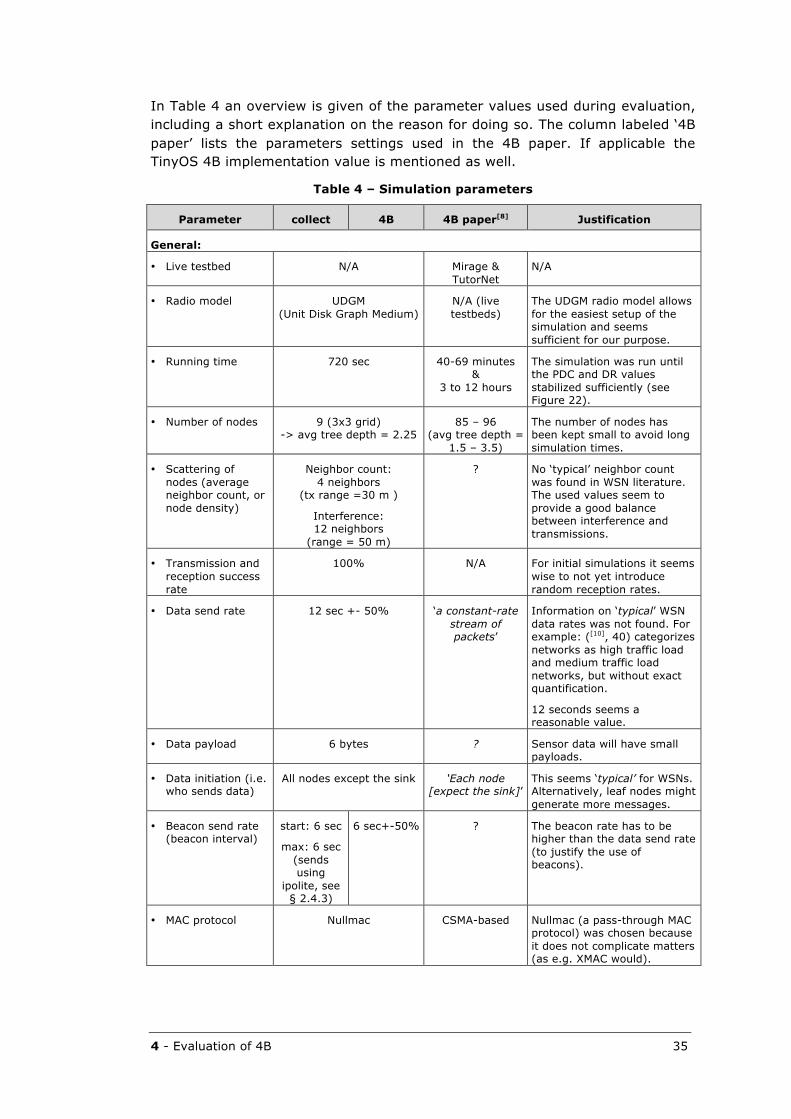
In Table 4 an overview is given of the parameter values used during evaluation, including a short explanation on the reason for doing so. The column labeled ‘4B paper’ lists the parameters settings used in the 4B paper. If applicable the TinyOS 4B implementation value is mentioned as well.
Table 4 – Simulation parameters
Parameter collect 4B 4B paper[8] Justification
General:
• Live testbed N/A Mirage & TutorNet
N/A
• Radio model UDGM (Unit Disk Graph Medium)
N/A (live testbeds)
The UDGM radio model allows for the easiest setup of the simulation and seems sufficient for our purpose.
• Running time 720 sec 40-69 minutes &
3 to 12 hours
The simulation was run until the PDC and DR values stabilized sufficiently (see Figure 22).
• Number of nodes 9 (3x3 grid) -> avg tree depth = 2.25
85 – 96 (avg tree depth =
1.5 – 3.5)
The number of nodes has been kept small to avoid long simulation times.
• Scattering of nodes (average neighbor count, or node density)
Neighbor count: 4 neighbors
(tx range =30 m )
Interference: 12 neighbors
(range = 50 m)
? No ‘typical’ neighbor count was found in WSN literature. The used values seem to provide a good balance between interference and transmissions.
• Transmission and reception success rate
100% N/A For initial simulations it seems wise to not yet introduce random reception rates.
• Data send rate 12 sec +- 50% ‘a constant-rate stream of packets’
Information on ‘typical’ WSN data rates was not found. For example: ([10], 40) categorizes networks as high traffic load and medium traffic load networks, but without exact quantification.
12 seconds seems a reasonable value.
• Data payload 6 bytes ? Sensor data will have small payloads.
• Data initiation (i.e. who sends data)
All nodes except the sink ‘Each node [expect the sink]’
This seems ‘typical’ for WSNs. Alternatively, leaf nodes might generate more messages.
• Beacon send rate (beacon interval)
start: 6 sec
max: 6 sec (sends using
ipolite, see § 2.4.3)
6 sec+-50% ? The beacon rate has to be higher than the data send rate (to justify the use of beacons).
• MAC protocol Nullmac CSMA-based Nullmac (a pass-through MAC protocol) was chosen because it does not complicate matters (as e.g. XMAC would).
36 4 - Evaluation of 4B
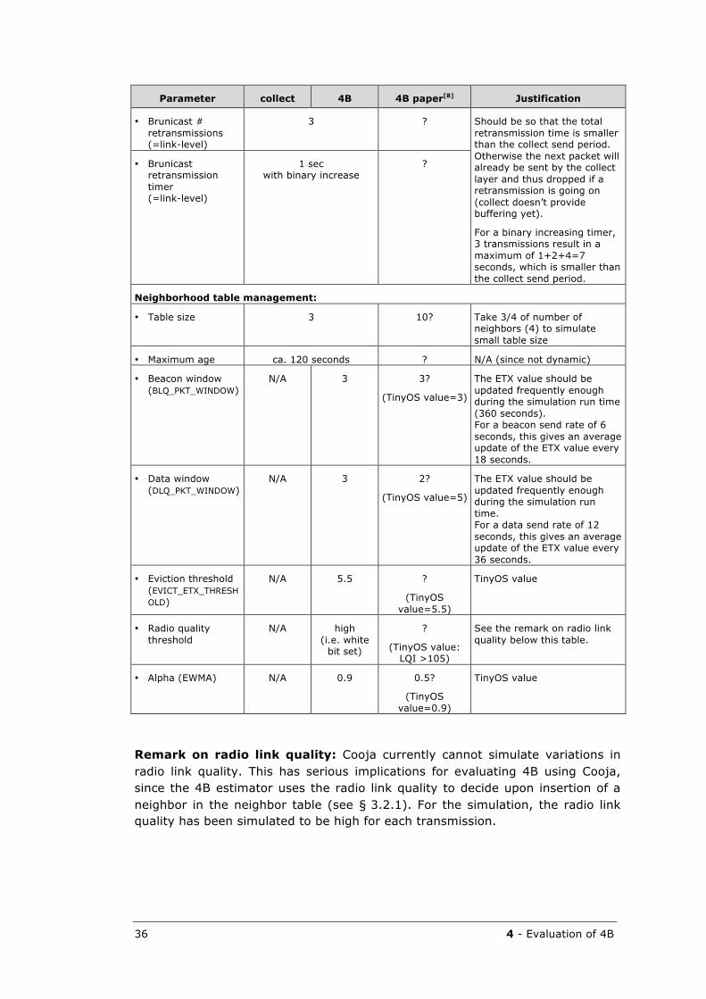
Parameter collect 4B 4B paper[8] Justification
• Brunicast # retransmissions (=link-level)
3 ?
• Brunicast retransmission timer (=link-level)
1 sec with binary increase
?
Should be so that the total retransmission time is smaller than the collect send period. Otherwise the next packet will already be sent by the collect layer and thus dropped if a retransmission is going on (collect doesn’t provide buffering yet).
For a binary increasing timer, 3 transmissions result in a maximum of 1+2+4=7 seconds, which is smaller than the collect send period.
Neighborhood table management:
• Table size 3 10? Take 3/4 of number of neighbors (4) to simulate small table size
• Maximum age ca. 120 seconds ? N/A (since not dynamic)
• Beacon window (BLQ_PKT_WINDOW)
N/A 3 3?
(TinyOS value=3)
The ETX value should be updated frequently enough during the simulation run time (360 seconds). For a beacon send rate of 6 seconds, this gives an average update of the ETX value every 18 seconds.
• Data window (DLQ_PKT_WINDOW)
N/A 3 2?
(TinyOS value=5)
The ETX value should be updated frequently enough during the simulation run time. For a data send rate of 12 seconds, this gives an average update of the ETX value every 36 seconds.
• Eviction threshold (EVICT_ETX_THRESHOLD)
N/A 5.5 ?
(TinyOS value=5.5)
TinyOS value
• Radio quality threshold
N/A high (i.e. white
bit set)
?
(TinyOS value: LQI >105)
See the remark on radio link quality below this table.
• Alpha (EWMA) N/A 0.9 0.5?
(TinyOS value=0.9)
TinyOS value
Remark on radio link quality: Cooja currently cannot simulate variations in radio link quality. This has serious implications for evaluating 4B using Cooja, since the 4B estimator uses the radio link quality to decide upon insertion of a neighbor in the neighbor table (see § 3.2.1). For the simulation, the radio link quality has been simulated to be high for each transmission.
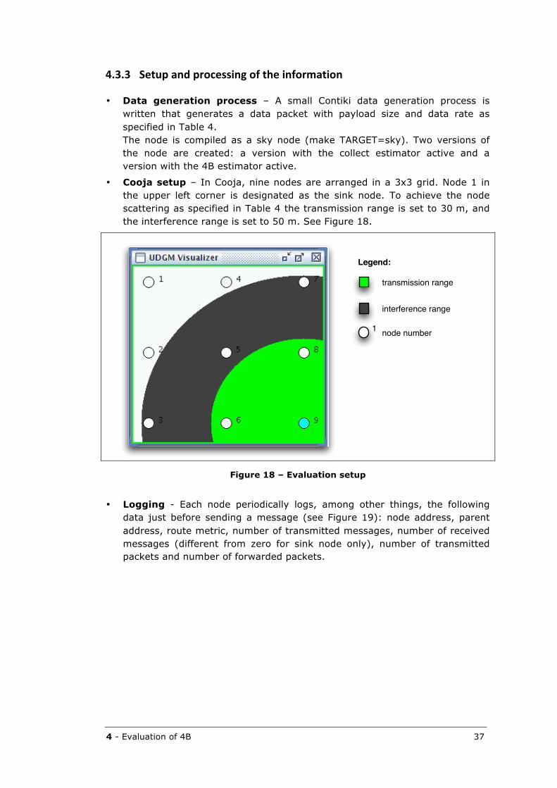
4 - Evaluation of 4B 37
4.3.3 Setupandprocessingoftheinformation
• Data generation process – A small Contiki data generation process is written that generates a data packet with payload size and data rate as specified in Table 4. The node is compiled as a sky node (make TARGET=sky). Two versions of the node are created: a version with the collect estimator active and a version with the 4B estimator active.
• Cooja setup – In Cooja, nine nodes are arranged in a 3x3 grid. Node 1 in the upper left corner is designated as the sink node. To achieve the node scattering as specified in Table 4 the transmission range is set to 30 m, and the interference range is set to 50 m. See Figure 18.
Figure 18 – Evaluation setup
• Logging - Each node periodically logs, among other things, the following data just before sending a message (see Figure 19): node address, parent address, route metric, number of transmitted messages, number of received messages (different from zero for sink node only), number of transmitted packets and number of forwarded packets.
Legend:
interference range
transmission range
node number1
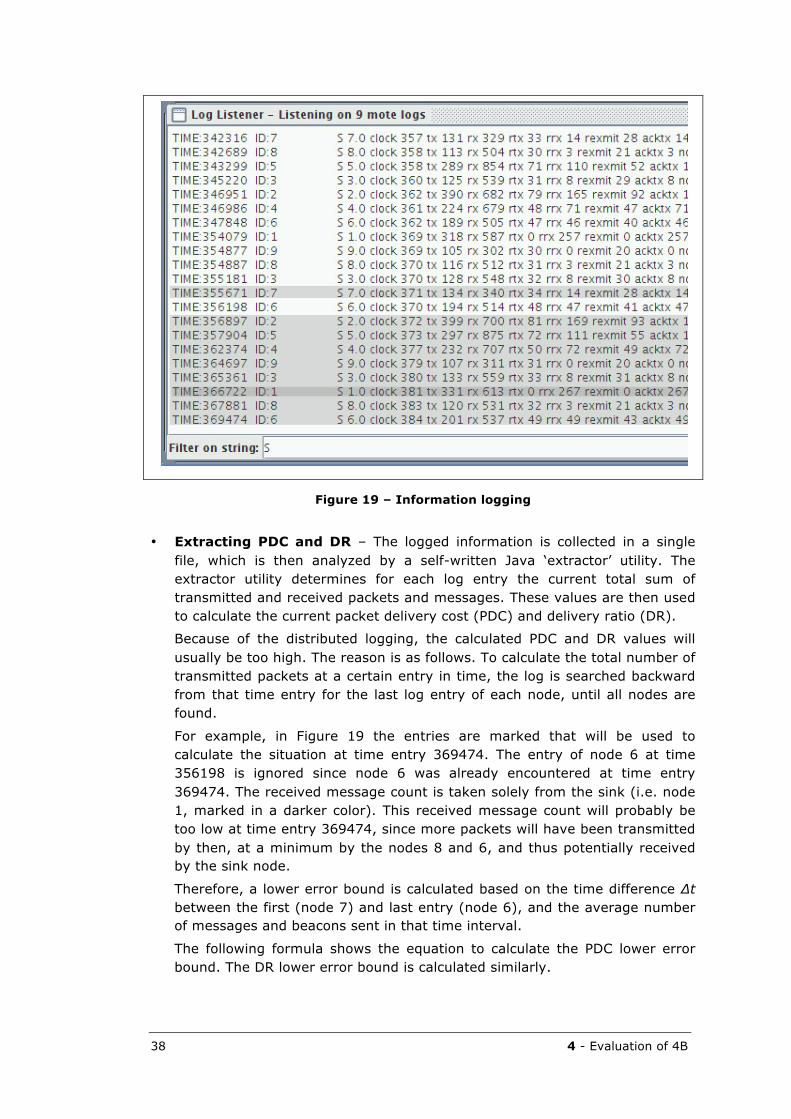
38 4 - Evaluation of 4B
Figure 19 – Information logging
• Extracting PDC and DR – The logged information is collected in a single file, which is then analyzed by a self-written Java ‘extractor’ utility. The extractor utility determines for each log entry the current total sum of transmitted and received packets and messages. These values are then used to calculate the current packet delivery cost (PDC) and delivery ratio (DR).
Because of the distributed logging, the calculated PDC and DR values will usually be too high. The reason is as follows. To calculate the total number of transmitted packets at a certain entry in time, the log is searched backward from that time entry for the last log entry of each node, until all nodes are found.
For example, in Figure 19 the entries are marked that will be used to calculate the situation at time entry 369474. The entry of node 6 at time 356198 is ignored since node 6 was already encountered at time entry 369474. The received message count is taken solely from the sink (i.e. node 1, marked in a darker color). This received message count will probably be too low at time entry 369474, since more packets will have been transmitted by then, at a minimum by the nodes 8 and 6, and thus potentially received by the sink node.
Therefore, a lower error bound is calculated based on the time difference ∆t between the first (node 7) and last entry (node 6), and the average number of messages and beacons sent in that time interval.
The following formula shows the equation to calculate the PDC lower error bound. The DR lower error bound is calculated similarly.
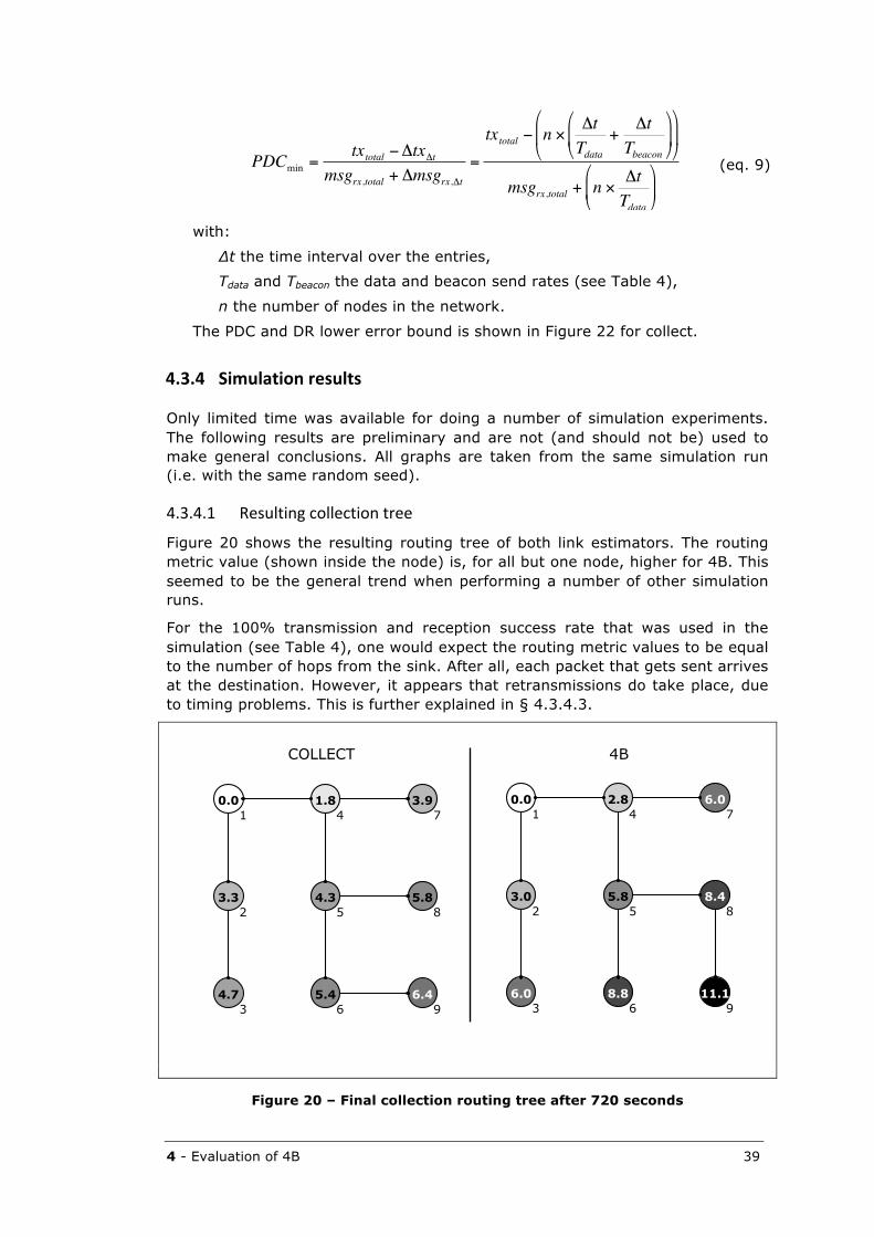
4 - Evaluation of 4B 39
€
PDCmin =txtotal −ΔtxΔt
msgrx,total + Δmsgrx,Δt=
txtotal − n × ΔtTdata
+Δt
Tbeacon
msgrx,total + n × ΔtTdata
(eq. 9)
with:
∆t the time interval over the entries,
Tdata and Tbeacon the data and beacon send rates (see Table 4),
n the number of nodes in the network.
The PDC and DR lower error bound is shown in Figure 22 for collect.
4.3.4 Simulationresults
Only limited time was available for doing a number of simulation experiments. The following results are preliminary and are not (and should not be) used to make general conclusions. All graphs are taken from the same simulation run (i.e. with the same random seed).
4.3.4.1 Resultingcollectiontree
Figure 20 shows the resulting routing tree of both link estimators. The routing metric value (shown inside the node) is, for all but one node, higher for 4B. This seemed to be the general trend when performing a number of other simulation runs.
For the 100% transmission and reception success rate that was used in the simulation (see Table 4), one would expect the routing metric values to be equal to the number of hops from the sink. After all, each packet that gets sent arrives at the destination. However, it appears that retransmissions do take place, due to timing problems. This is further explained in § 4.3.4.3.
Figure 20 – Final collection routing tree after 720 seconds
COLLECT 4B
0.01
3.32
4.73
1.84
4.35
5.46
3.97
5.88
6.49
0.01
3.02
6.03
2.84
5.85
8.86
6.07
8.48
11.19
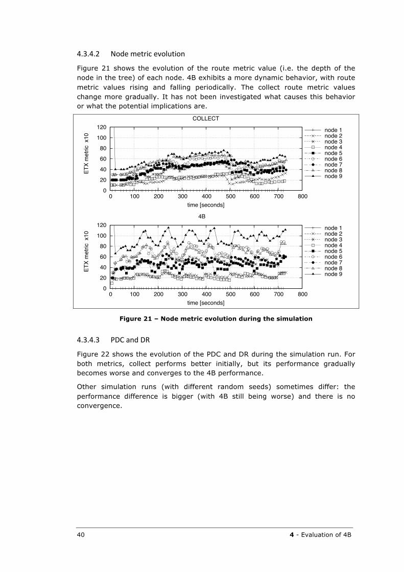
40 4 - Evaluation of 4B
4.3.4.2 Nodemetricevolution
Figure 21 shows the evolution of the route metric value (i.e. the depth of the node in the tree) of each node. 4B exhibits a more dynamic behavior, with route metric values rising and falling periodically. The collect route metric values change more gradually. It has not been investigated what causes this behavior or what the potential implications are.
Figure 21 – Node metric evolution during the simulation
4.3.4.3 PDCandDR
Figure 22 shows the evolution of the PDC and DR during the simulation run. For both metrics, collect performs better initially, but its performance gradually becomes worse and converges to the 4B performance.
Other simulation runs (with different random seeds) sometimes differ: the performance difference is bigger (with 4B still being worse) and there is no convergence.
0
20
40
60
80
100
120
0 100 200 300 400 500 600 700 800
ETX
met
ric x
10
time [seconds]
COLLECT
node 1node 2node 3node 4node 5node 6node 7node 8 node 9
0
20
40
60
80
100
120
0 100 200 300 400 500 600 700 800
ETX
met
ric x
10
time [seconds]
4B
node 1 node 2 node 3 node 4 node 5 node 6 node 7 node 8 node 9
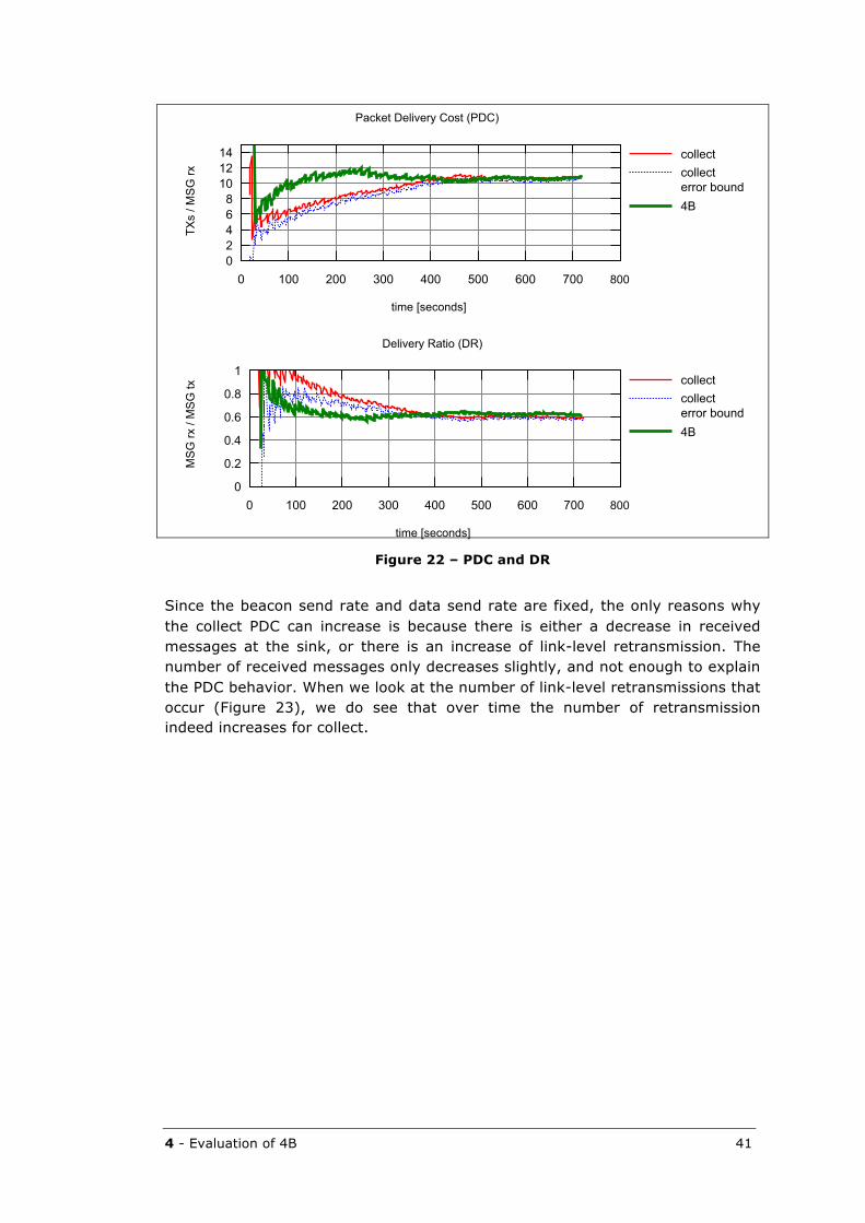
4 - Evaluation of 4B 41
Figure 22 – PDC and DR
Since the beacon send rate and data send rate are fixed, the only reasons why the collect PDC can increase is because there is either a decrease in received messages at the sink, or there is an increase of link-level retransmission. The number of received messages only decreases slightly, and not enough to explain the PDC behavior. When we look at the number of link-level retransmissions that occur (Figure 23), we do see that over time the number of retransmission indeed increases for collect.
02468
101214
0 100 200 300 400 500 600 700 800
TXs
/ MSG
rx
time [seconds]
Packet Delivery Cost (PDC)
collectcollect error bound4B
0
0.2
0.4
0.6
0.8
1
0 100 200 300 400 500 600 700 800
MSG
rx /
MSG
tx
time [seconds]
Delivery Ratio (DR)
collectcollecterror bound4B
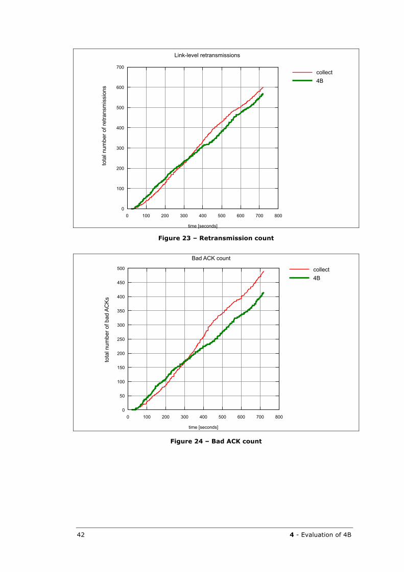
42 4 - Evaluation of 4B
Figure 23 – Retransmission count
Figure 24 – Bad ACK count
0
100
200
300
400
500
600
700
0 100 200 300 400 500 600 700 800
tota
l num
ber o
f ret
rans
mis
sion
s
time [seconds]
Link-level retransmissions
collect4B
0
50
100
150
200
250
300
350
400
450
500
0 100 200 300 400 500 600 700 800
tota
l num
ber o
f bad
AC
Ks
time [seconds]
Bad ACK count
collect4B
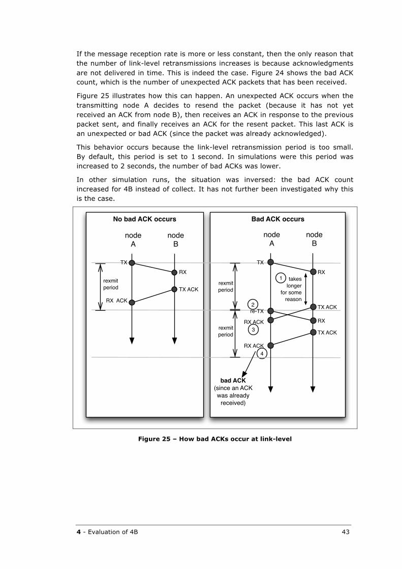
4 - Evaluation of 4B 43
If the message reception rate is more or less constant, then the only reason that the number of link-level retransmissions increases is because acknowledgments are not delivered in time. This is indeed the case. Figure 24 shows the bad ACK count, which is the number of unexpected ACK packets that has been received.
Figure 25 illustrates how this can happen. An unexpected ACK occurs when the transmitting node A decides to resend the packet (because it has not yet received an ACK from node B), then receives an ACK in response to the previous packet sent, and finally receives an ACK for the resent packet. This last ACK is an unexpected or bad ACK (since the packet was already acknowledged).
This behavior occurs because the link-level retransmission period is too small. By default, this period is set to 1 second. In simulations were this period was increased to 2 seconds, the number of bad ACKs was lower.
In other simulation runs, the situation was inversed: the bad ACK count increased for 4B instead of collect. It has not further been investigated why this is the case.
Figure 25 – How bad ACKs occur at link-level
2
3
4
No bad ACK occurs Bad ACK occurs
rexmitperiod
rexmitperiod
rexmitperiod
takeslonger
for somereason
1
nodeA
nodeB
TX
RX ACK
RX
TX ACK
nodeA
nodeB
TX
RX ACK
RX
TX ACK re-TX
RX ACK
TX ACK
RX
bad ACK(since an ACKwas already
received)
44 4 - Evaluation of 4B
4.4 Evaluation
4.4.1 Packetdeliverycost(PDC)anddeliveryratio(DR)
The PDC and DR results were discussed in § 4.3.4.3. As mentioned, collect performed better initially but ultimately worsens to converge to 4B’s performance. This shows that the implemented 4B link estimator is functional, but unfortunately the limited simulations do not allow drawing quantitative conclusions.
4.4.2 Memoryrequirements
Memory requirements can be split up in static memory (ROM) and dynamic memory (RAM) required.
4.4.2.1 Staticmemoryrequired
If we compare the compiled file size of a node with either collect or 4B included (Table 5), we see that 4B requires almost 12 kilobytes more memory.
The comparison is a bit unfair however, since 4B has its own beacon-sending module but still has the Rime announcement primitive included. 4B’s compile size could be optimized by using the announcement primitive as well.
Table 5 – Static memory requirements
Collect 4B
Compiled file size 370.611 bytes 382.589 bytes
4.4.2.2 Dynamicmemoryrequired
The dynamic memory required is determined by the neighbor table fields and the number of neighbors. Since the number of neighbors depends on the deployment, it is important that the fields consume as little memory as possible.
As we can see in Table 6, both memory requirements are more or less on par. Whereas the collect approach has less fields than 4B, the ETX history table (etxs[8]) takes up a lot of space. For a hypothetical node with 10 neighbors, the difference would be about 20 bytes, which is negligible.
However, there is potential to reduce the memory requirement of the collect estimator by replacing the 8-history ETX table with the EWMA-approach of 4B (see § 3.2.2). This would require storing only an 8-bit ETX value, leaving the collect estimator happy with a total of only 48 bits per neighbor entry (instead of 112 bits).
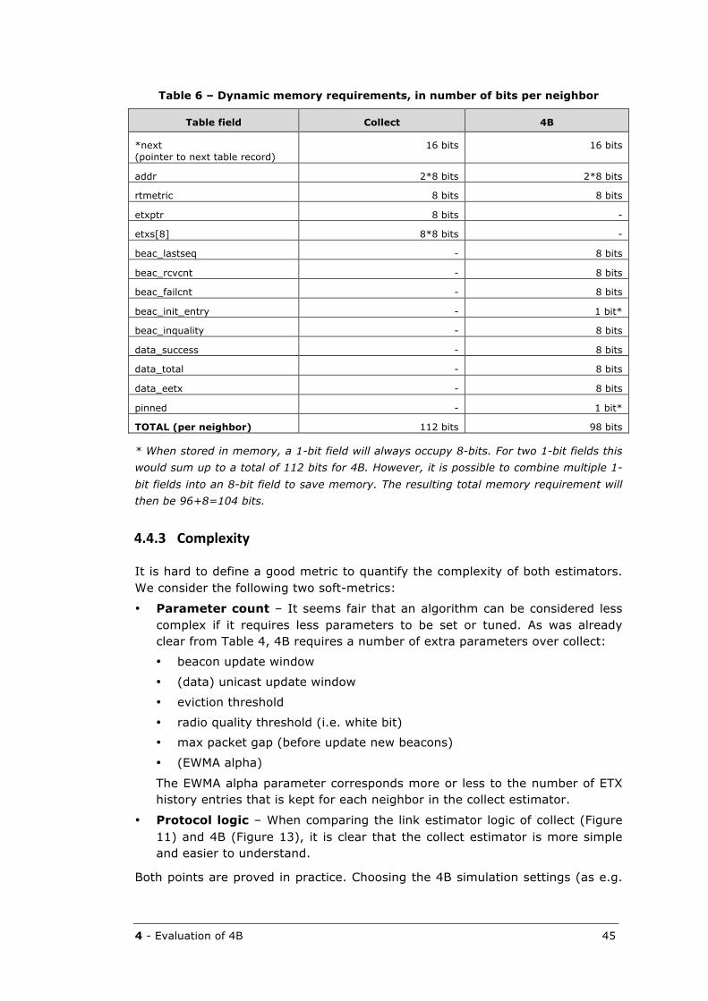
4 - Evaluation of 4B 45
Table 6 – Dynamic memory requirements, in number of bits per neighbor
Table field Collect 4B
*next (pointer to next table record)
16 bits 16 bits
addr 2*8 bits 2*8 bits
rtmetric 8 bits 8 bits
etxptr 8 bits -
etxs[8] 8*8 bits -
beac_lastseq - 8 bits
beac_rcvcnt - 8 bits
beac_failcnt - 8 bits
beac_init_entry - 1 bit*
beac_inquality - 8 bits
data_success - 8 bits
data_total - 8 bits
data_eetx - 8 bits
pinned - 1 bit*
TOTAL (per neighbor) 112 bits 98 bits
* When stored in memory, a 1-bit field will always occupy 8-bits. For two 1-bit fields this would sum up to a total of 112 bits for 4B. However, it is possible to combine multiple 1-bit fields into an 8-bit field to save memory. The resulting total memory requirement will then be 96+8=104 bits.
4.4.3 Complexity
It is hard to define a good metric to quantify the complexity of both estimators. We consider the following two soft-metrics:
• Parameter count – It seems fair that an algorithm can be considered less complex if it requires less parameters to be set or tuned. As was already clear from Table 4, 4B requires a number of extra parameters over collect:
• beacon update window
• (data) unicast update window
• eviction threshold
• radio quality threshold (i.e. white bit)
• max packet gap (before update new beacons)
• (EWMA alpha)
The EWMA alpha parameter corresponds more or less to the number of ETX history entries that is kept for each neighbor in the collect estimator.
• Protocol logic – When comparing the link estimator logic of collect (Figure 11) and 4B (Figure 13), it is clear that the collect estimator is more simple and easier to understand.
Both points are proved in practice. Choosing the 4B simulation settings (as e.g.
46 4 - Evaluation of 4B
Table 4) was not easy, especially in absence of real network properties such as required or average data send rate. Also, due to the complexity of 4B, its implementation required painful debugging and verification of its operation under various scenarios.
So, it seems reasonable to consider 4B more complex than collect.
4.5 Conclusion
From the limited evaluations performed in this section, it cannot be concluded that the 4B estimator performs better, or worse, than the collect estimator.
The number of simulations performed to evaluate the packet delivery cost of 4B are too limited and not representative and conclusions cannot be drawn from them. Moreover, the Cooja network simulator currently does not provide radio link quality simulation, which limits the scope of the simulation as well.
Both estimators are on par with each other what concerns memory requirements. 4B however, is more complex than collect. This potentially results in an increased code size and implementation bugs.
5 - Thesis evaluation 47
5 Thesisevaluation
In this section a short overview is given on the actions taken while working on this thesis, and of the problems encountered during this work.
5.1 Thesisprogress
The following paragraphs give a brief summary on the progress and actions taken while working on this thesis.
During September-October-November I took up C programming, installed Contiki/Cooja, and created an ‘how to install’ tutorial in the progress (see § 8.1). I played around with simple Contiki ‘Hello World’ programs, and simple broadcasts to neighbors.
During February-March I read up on relevant papers, studied the Rime protocol stack, analyzed how 4B could be mapped on the Rime stack and studied the high-level workings of the collect protocol. I played around with Sentilla nodes (uploading and running simple programs), creating a tutorial in the progress (see § 8.2). Unfortunately, this work turned out to be in vain since the 4B implementation was not tested on real Sentilla nodes in the end.
During April-May, I studied (and documented) the details of the Contiki collect protocol, studied the details of the TinyOS 4B implementation, implemented 4B in Contiki, studied the workings of the announcement module, evaluated my 4B implementation, wrote some Java tools to simplify evaluation data processing, and wrote this document.
5.2 Problemsencountered
Progress for thesis was slower than I had anticipated. I attribute this to the following issues:
• Documentation – The Contiki operating system is a young and fast-moving project. As a result, documentation (source-code and otherwise) isn’t always as expected. Sometimes it is outdated, a lot of times it is very limited or missing. This makes it time-consuming to get up to date with the available features, how to use them, and in general to ‘dive into the code’.
• C knowledge minimal – My knowledge of the C programming language was theoretical, at best. Getting comfortable with the confusing syntax for pointers to structs, functions and all-other-things-in-the-universe took some time.
48 5 - Thesis evaluation
• Continuously patched – The Contiki source code is continuously extended and patched. While this is in general a good thing, it can slow down progress if the bug fixes affect my own modified code, which then has to be re-evaluated as well.
• Quite some bugs – The number of bugs I encountered (see § 8.5) made me be very critical about all lines of code I investigated. This makes for slower progress than if one has more confidence on the code; on the positive side, it makes for better code!
• Cooja – The documentation of Cooja is also lacking to non-existing. It is difficult to get a view on the features and on how to use Cooja in the most appropriate way possible. Also, it appears that some ‘essential features’ are not yet available (like directly logging to a file). This resulted in putting work in writing some tools and extensions to make up for these missing features.
• 4B paper – The 4B paper[8] was less explicit and clear about the exact estimator implementation than we had assumed. This required studying the TinyOS implementation to get all the required details of the algorithm.
However, it is undoubtedly in a large part due to these problems encountered that the work became interesting and challenging!

6 - Conclusion and further work 49
6 Conclusionandfurtherwork
6.1 Conclusion
The initial goal of this work was to implement the four-bit wireless link estimator (4B) in the Contiki data collection protocol, followed by an evaluation against the current Contiki link estimator. The reason for this was twofold:
• validate or refute the proclaimed results of 4B,
• improve the Contiki collection protocol by including a better link estimator.
It was realized however that the implementation details of 4B were not clear from the paper alone and that the time frame was not sufficient for a full implementation and evaluation in Contiki.
First, the Contiki collect protocol was studied and described in detail, since it is the link estimator in this protocol that has to be replaced by the 4B estimator. A detailed study of the 4B TinyOS implementation was required to uncover all details of 4B. Following this work, the 4B estimator has been documented in detail.
Building on this theoretical study, we investigated which metrics can be used to evaluate the performance of both link estimators. To evaluate the packet delivery cost of both estimators, we set out the conditions under which a simulation can take place, and performed some initial simulations. These simulations were too limited to reveal any useful results.
Regarding other metrics, we showed that the memory footprint of 4B is similar to the memory footprint of the current collect link estimator. The 4B estimator does have a higher complexity, potentially leading to a more complex parameter-tuning problem.
6.2 Furtherwork
As a direct follow-up to this work the following are obvious suggestions for further work:
• Implement 4B in Contiki with a stricter separation from the current collection protocol.
• For evaluation in Cooja, it is required that varying radio link quality can be simulated. This should be implemented in Cooja.
• Perform a thorough evaluation of this implementation, both in Cooja and on a live testbed.
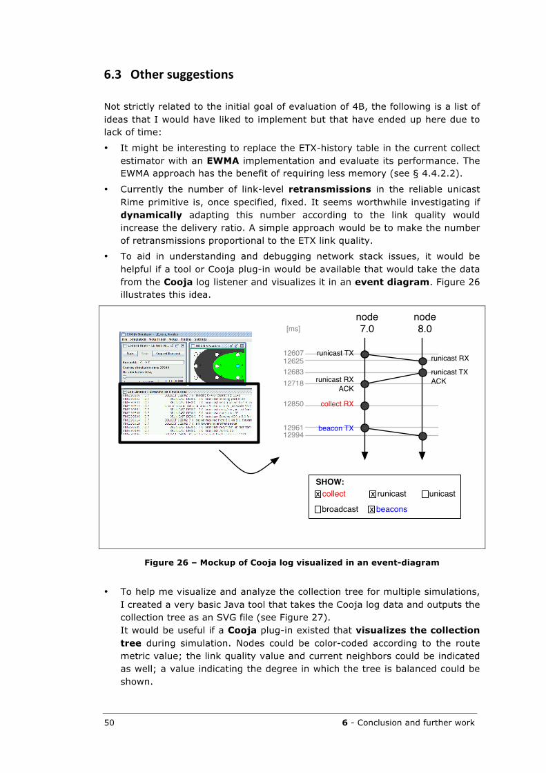
50 6 - Conclusion and further work
6.3 Othersuggestions
Not strictly related to the initial goal of evaluation of 4B, the following is a list of ideas that I would have liked to implement but that have ended up here due to lack of time:
• It might be interesting to replace the ETX-history table in the current collect estimator with an EWMA implementation and evaluate its performance. The EWMA approach has the benefit of requiring less memory (see § 4.4.2.2).
• Currently the number of link-level retransmissions in the reliable unicast Rime primitive is, once specified, fixed. It seems worthwhile investigating if dynamically adapting this number according to the link quality would increase the delivery ratio. A simple approach would be to make the number of retransmissions proportional to the ETX link quality.
• To aid in understanding and debugging network stack issues, it would be helpful if a tool or Cooja plug-in would be available that would take the data from the Cooja log listener and visualizes it in an event diagram. Figure 26 illustrates this idea.
Figure 26 – Mockup of Cooja log visualized in an event-diagram
• To help me visualize and analyze the collection tree for multiple simulations, I created a very basic Java tool that takes the Cooja log data and outputs the collection tree as an SVG file (see Figure 27). It would be useful if a Cooja plug-in existed that visualizes the collection tree during simulation. Nodes could be color-coded according to the route metric value; the link quality value and current neighbors could be indicated as well; a value indicating the degree in which the tree is balanced could be shown.
12607126251268312718
12850
1296112994
node7.0
node8.0
runicast TX
runicast RX ACK
runicast RX
runicast TX ACK
collect RX
beacon TX
[ms]
SHOW:x collect x runicast unicast
broadcast x beacons
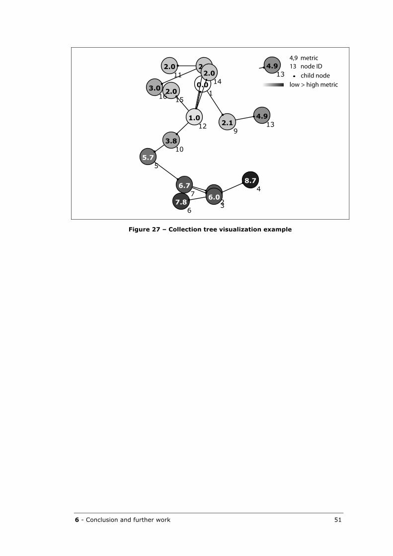
6 - Conclusion and further work 51
Figure 27 – Collection tree visualization example
0.01
6.52
6.03
8.74
5.75
7.86
6.77
2.08
2.19
3.810
2.011
1.012
4.913
4.9132.0
142.015
3.016
4,9 metric13 node ID child nodelow > high metric

52 6 - Conclusion and further work

7 - Literature 53
7 Literature
[1] Contiki Doxygen documentation, main page, http://www.sics.se/~adam/contiki/docs/main.html, retrieved 2009-05-09
[2] Contiki website, http://www.sics.se/contiki/about-contiki.html, retrieved 2009-05-09
[3] Adam Dunkels: “Announcement.c module questions”, Contiki developer mailing list, 2009-04-07
[4] Adam Dunkels, Björn Grönvall, and Thiemo Voigt: Contiki - a Lightweight and Flexible Operating System for Tiny Networked Sensors, Local Computer Networks, 2004. 29th Annual IEEE International Conference, page 455-462, 2004
[5] Adam Dunkels, Fredrik Österlind, and Zhitao He: An Adaptive Communication Architecture for Wireless Sensor Networks, Proceedings of the 5th international conference on Embedded networked sensors systems, page 335-349, 2007
[6] Adam Dunkels, Fredrik Österlind, Nicolas Tsiftes: IP-based Sensor Networking with Contiki, ACM/IEEE conference on Information Processing in Sensor Networks (IPSN), April 16th 2009
[7] Douglas S. J. De Couto: High-Throughput Routing for Multi-Hop Wireless Networks, 2004
[8] Rodrigo Fonseca, Omprakash Gnawali, Kyle Jamieson, Philip Levis, Four-Bit: Wireless Link Estimation, Proc. Of the ACM HotNets-VI Conf., 2007
[9] IEEE Standard. 802.15.4 - 2003: Wireless Medium Access Control (MAC) and Physical Layer (PHY) Specifications for Low Rate Wireless Personal Area Networks (LR-WPANs) http://standards.ieee.org/getieee802/download/802.15.4-2003.pdf
[10] Raja Jurdak: Wireless Ad Hoc and Sensor Network – a cross-layer design perspective, Springer 2007
[11] Philip Levis, Eric Brewer, David Culler, David Gay, Sam Madden, Neil Patel, Joe Polastre, Scott Shenker, Robert Szewczyk, Alec Woo: The Emergence of a Networking Primitive in Wireless Sensor Networks, Communications of the ACM Volume 51, Number 7, July 2008
[12] Tao Li, Ankur Kamthe, Lun Jiang and Alberto Cerpa: Performance Evaluation of Link Quality Estimation Metrics for Static MultiHop Wireless Sensor Networks, to appear in SECON 2009, June 2009, http://www.andes.ucmerced.edu/research/linkmetrics.html, retrieved 2009-04-03
[13] Optimized Autonomous Space In-Situ Sensorweb, Vulcano hazard monitoring picture http://www.vancouver.wsu.edu/fac/song/images/oasis.JPG, retrieved 2005-05-15
[14] Bhaskaran Raman, Kameswari Chebrolu: Censor Networks - A Critique of “Sensor Networks” from a Systems Perspective, ACM SIGCOMM Computer Communication Review Volume 38, Number 3, July 2008
[15] Kay Romer and Friedemann Mattern: The Design Space of Wireless Sensor Networks, IEEE Wireless Communications, 2004
54 7 - Literature
[16] Texas Instruments CC2420, 2,4GHz IEEE 802;15;4 / ZigBee-ready RF Transceiver, http://focus.ti.com/lit/ds/symlink/cc2420.pdf, retrieved on 2009-05-16
[17] TinyOS Extension Proposal (TEP) 119, Collection, http://www.tinyos.net/tinyos-2.x/doc/html/tep119.html
[18] TinyOS Extension Proposal (TEP) 123, The Collection Tree Protocol (CTP), http://www.tinyos.net/tinyos-2.x/doc/html/tep123.html
[19] TinyOS Extension Proposal (TEP) 124, Link Estimation Exchange Protocol (LEEP), http://www.tinyos.net/tinyos-2.x/doc/html/tep124.html
[20] Alec Woo, Terence Tong, David Culler: Taming the Underlying Challenges of Reliable Multihop Routing in Sensor Networks, Proceedings of the 1st international conference on Embedded networked sensor systems, pages 14-27, 2003

8 - Appendix 55
8 Appendix
8.1 AppendixA–Tutorial‘InstallingContiki/CoojaonUbuntu8.10’
This tutorial shows how to install Contiki 2.2.2 and Cooja on a fresh Ubuntu 8.10 system. There should be no (major) differences for Contiki 2.2.1 and/or Ubuntu 8.04.
Don't be put off by the length of this tutorial: for clarity it lists every step. If you are proficient with *nix, cvs, ant and the like, you will walk through it in less than 5 minutes. If you are less experienced, it provides enough detail to get you up and running with Contiki and Cooja.
Step 1: Get Contiki There are several options to get Contiki. An overview is available at the download page. This step describes two methods: (a) downloading Contiki as a zip file, or (b) checking it out from the CVS repository. Method b provides an easy way to stay up to date with the latest changes to Contiki.
To continue, choose either step 1A or 1B.
STEP 1A) downloading zip file
1. Download Contiki from the Download page (http://www.sics.se/contiki/download.html).
2. Unzip Contiki to (for example) your Desktop.
STEP 1B) checking out from the CVS repository
CVS is by default not installed on Ubuntu (typing cvs in a terminal will tell you so).
1. Install CVS by typing:
sudo apt-get install cvs
2. Checkout (download) the contiki files from the CVS repository:
cd Desktop (or any other folder you like) cvs -z3 -d:pserver:[email protected]:/cvsroot/contiki co contiki-2.x
This will create a folder contiki-2.x on your Desktop. The -z3 argument is optional and specifies to use level 3 compression. The -d argument allows you to specify the location of the CVS root (an alternative would be to set the CVSROOT environment variable, consult the CVS man page for more information). The co argument is shorthand for checkout. The argument contiki-2.x is the module (i.e. folder) to be checked out from the repository.
Remarks:
• To keep your local copy updated with the latest changes from the CVS repository, cd into the folder that you want to update (either contiki-2.x or a particular subfolder) and type:
cd contiki-2.x (or a particular subfolder) cvs update -dP
Quoting the cvs man pages: -P Prune empty directories. -d Create any directories that exist in the repository if they're missing from the working directory. Normally, update acts only on directories and files that were already enrolled in your working directory.
• More information on the sourceforge CVS. The Contiki download page also provides a link to a page with more information about the Contiki CVS.
• The next steps assume you have downloaded contiki-2.2.2 as a zip file. If instead you have used the CVS method to get Contiki, type contiki-2.x anywhere contiki-2.2.2 is mentioned.
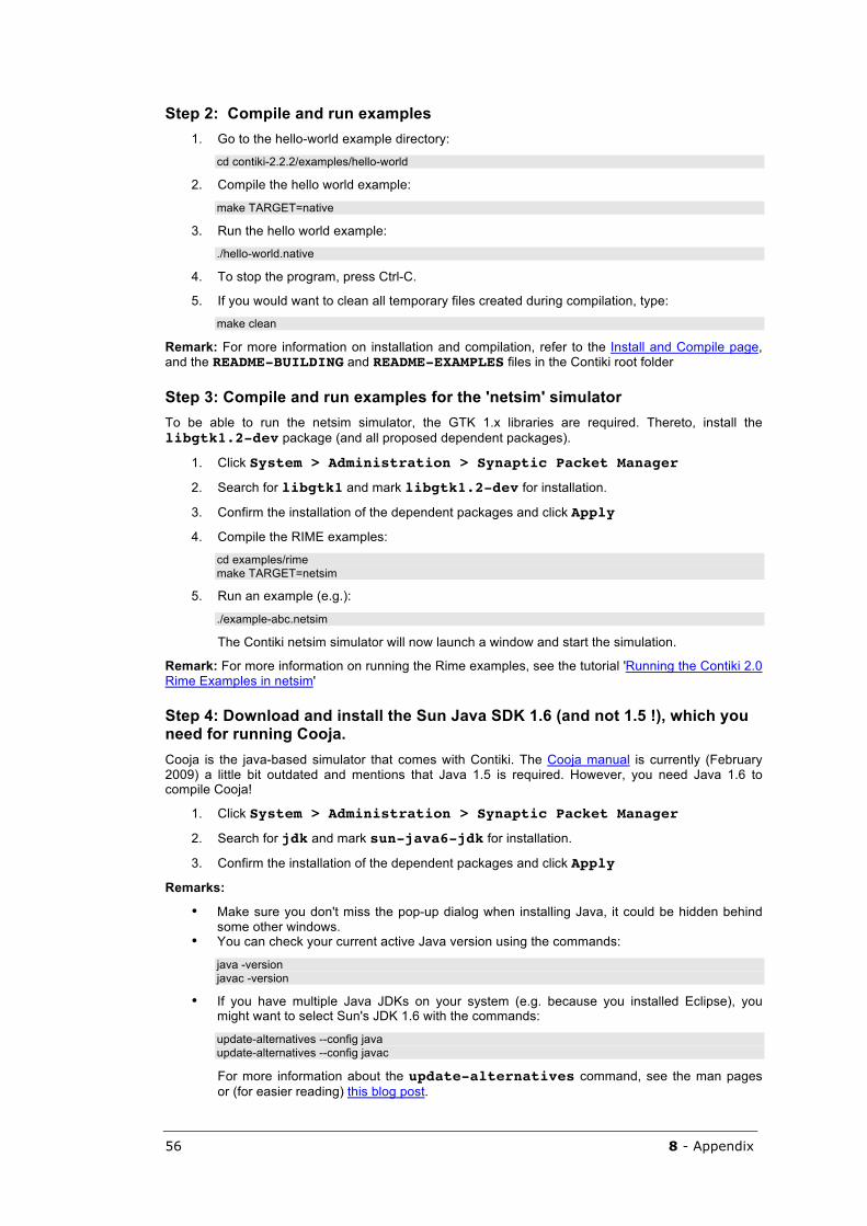
56 8 - Appendix
Step 2: Compile and run examples 1. Go to the hello-world example directory:
cd contiki-2.2.2/examples/hello-world
2. Compile the hello world example:
make TARGET=native
3. Run the hello world example:
./hello-world.native
4. To stop the program, press Ctrl-C.
5. If you would want to clean all temporary files created during compilation, type:
make clean
Remark: For more information on installation and compilation, refer to the Install and Compile page, and the README-BUILDING and README-EXAMPLES files in the Contiki root folder
Step 3: Compile and run examples for the 'netsim' simulator To be able to run the netsim simulator, the GTK 1.x libraries are required. Thereto, install the libgtk1.2-dev package (and all proposed dependent packages).
1. Click System > Administration > Synaptic Packet Manager
2. Search for libgtk1 and mark libgtk1.2-dev for installation.
3. Confirm the installation of the dependent packages and click Apply
4. Compile the RIME examples:
cd examples/rime make TARGET=netsim
5. Run an example (e.g.):
./example-abc.netsim
The Contiki netsim simulator will now launch a window and start the simulation.
Remark: For more information on running the Rime examples, see the tutorial 'Running the Contiki 2.0 Rime Examples in netsim'
Step 4: Download and install the Sun Java SDK 1.6 (and not 1.5 !), which you need for running Cooja. Cooja is the java-based simulator that comes with Contiki. The Cooja manual is currently (February 2009) a little bit outdated and mentions that Java 1.5 is required. However, you need Java 1.6 to compile Cooja!
1. Click System > Administration > Synaptic Packet Manager
2. Search for jdk and mark sun-java6-jdk for installation.
3. Confirm the installation of the dependent packages and click Apply
Remarks:
• Make sure you don't miss the pop-up dialog when installing Java, it could be hidden behind some other windows.
• You can check your current active Java version using the commands:
java -version javac -version
• If you have multiple Java JDKs on your system (e.g. because you installed Eclipse), you might want to select Sun's JDK 1.6 with the commands:
update-alternatives --config java update-alternatives --config javac
For more information about the update-alternatives command, see the man pages or (for easier reading) this blog post.
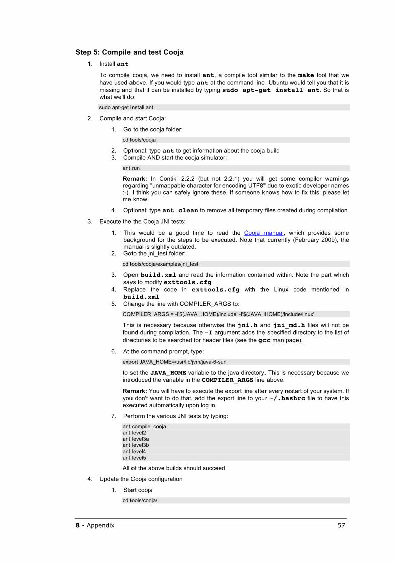
8 - Appendix 57
Step 5: Compile and test Cooja 1. Install ant
To compile cooja, we need to install ant, a compile tool similar to the make tool that we have used above. If you would type ant at the command line, Ubuntu would tell you that it is missing and that it can be installed by typing sudo apt-get install ant. So that is what we'll do:
sudo apt-get install ant
2. Compile and start Cooja:
1. Go to the cooja folder:
cd tools/cooja
2. Optional: type ant to get information about the cooja build 3. Compile AND start the cooja simulator:
ant run
Remark: In Contiki 2.2.2 (but not 2.2.1) you will get some compiler warnings regarding "unmappable character for encoding UTF8" due to exotic developer names :-). I think you can safely ignore these. If someone knows how to fix this, please let me know.
4. Optional: type ant clean to remove all temporary files created during compilation
3. Execute the the Cooja JNI tests:
1. This would be a good time to read the Cooja manual, which provides some background for the steps to be executed. Note that currently (February 2009), the manual is slightly outdated.
2. Goto the jni_test folder:
cd tools/cooja/examples/jni_test
3. Open build.xml and read the information contained within. Note the part which says to modify exttools.cfg
4. Replace the code in exttools.cfg with the Linux code mentioned in build.xml
5. Change the line with COMPILER_ARGS to:
COMPILER_ARGS = -I'$(JAVA_HOME)/include' -I'$(JAVA_HOME)/include/linux'
This is necessary because otherwise the jni.h and jni_md.h files will not be found during compilation. The -I argument adds the specified directory to the list of directories to be searched for header files (see the gcc man page).
6. At the command prompt, type:
export JAVA_HOME=/usr/lib/jvm/java-6-sun
to set the JAVA_HOME variable to the java directory. This is necessary because we introduced the variable in the COMPILER_ARGS line above.
Remark: You will have to execute the export line after every restart of your system. If you don't want to do that, add the export line to your ~/.bashrc file to have this executed automatically upon log in.
7. Perform the various JNI tests by typing:
ant compile_cooja ant level2 ant level3a ant level3b ant level4 ant level5
All of the above builds should succeed.
4. Update the Cooja configuration
1. Start cooja
cd tools/cooja/
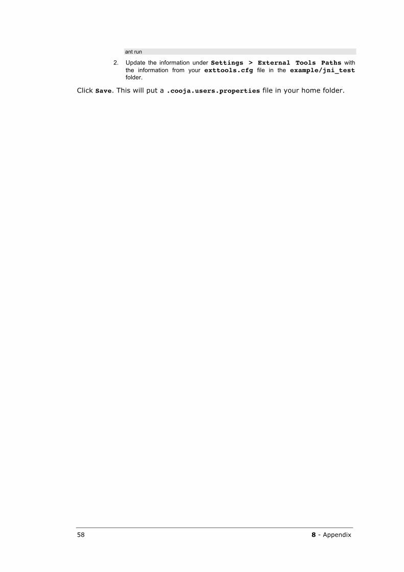
58 8 - Appendix
ant run
2. Update the information under Settings > External Tools Paths with the information from your exttools.cfg file in the example/jni_test folder.
Click Save. This will put a .cooja.users.properties file in your home folder.
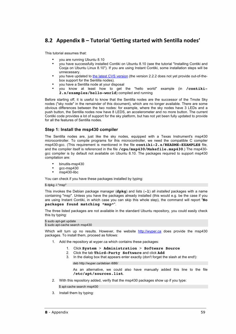
8 - Appendix 59
8.2 AppendixB–Tutorial‘GettingstartedwithSentillanodes’
This tutorial assumes that:
• you are running Ubuntu 8.10 • you have successfully installed Contiki on Ubuntu 8.10 (see the tutorial "Installing Contiki and
Cooja on Ubuntu Linux 8.10"). If you are using Instant Contiki, some installation steps will be unnecessary.
• you have updated to the latest CVS version (the version 2.2.2 does not yet provide out-of-the-box support for the Sentilla nodes).
• you have a Sentilla node at your disposal • you know at least how to get the "hello world" example (in /contiki-
2.x/examples/hello-world) compiled and running
Before starting off, it is useful to know that the Sentilla nodes are the successor of the Tmote Sky nodes ("sky node" in the remainder of this document), which are no longer available. There are some obvious differences between the two nodes: for example, where the sky nodes have 3 LEDs and a push button, the Sentilla nodes now have 8 LEDS, an accelerometer and no more button. The current Contiki code provides a lot of support for the sky platform, but has not yet been fully updated to provide for all the features of Sentilla nodes.
Step 1: Install the msp430 compiler The Sentilla nodes are, just like the sky nodes, equipped with a Texas Instrument's msp430 microcontroller. To compile programs for this microcontroller, we need the compatible C compiler msp430-gcc. (This requirement is mentioned in the file contiki-2.x/README-EXAMPLES file, and the compiler itself is referenced in the file /cpu/msp430/Makefile.msp430.) The msp430-gcc compiler is by default not available on Ubuntu 8.10. The packages required to support msp430 compilation are:
• binutils-msp430 • gcc-msp430 • msp430-libc
You can check if you have these packages installed by typing:
$ dpkg -l *msp*
This invokes the Debian package manager (dpkg) and lists (-l) all installed packages with a name containing "msp". Unless you have the packages already installed (this would e.g. be the case if you are using Instant Contiki, in which case you can skip this whole step), the command will report "No packages found matching *msp*".
The three listed packages are not available in the standard Ubuntu repository, you could easily check this by typing:
$ sudo apt-get update $ sudo apt-cache search msp430
Which will turn up no results. However, the website http://wyper.ca does provide the msp430 packages. To install them, proceed as follows:
1. Add the repository at wyper.ca which contains these packages:
1. Click System > Administration > Software Source 2. Click the tab Third-Party Software and click Add 3. In the dialog box that appears enter exactly (don't forget the slash at the end!):
deb http://wyper.ca/debian i686/
As an alternative, we could also have manually added this line to the file /etc/apt/sources.list.
2. With this repository added, verify that the msp430 packages show up if you type:
$ apt-cache search msp430
3. Install them by typing:
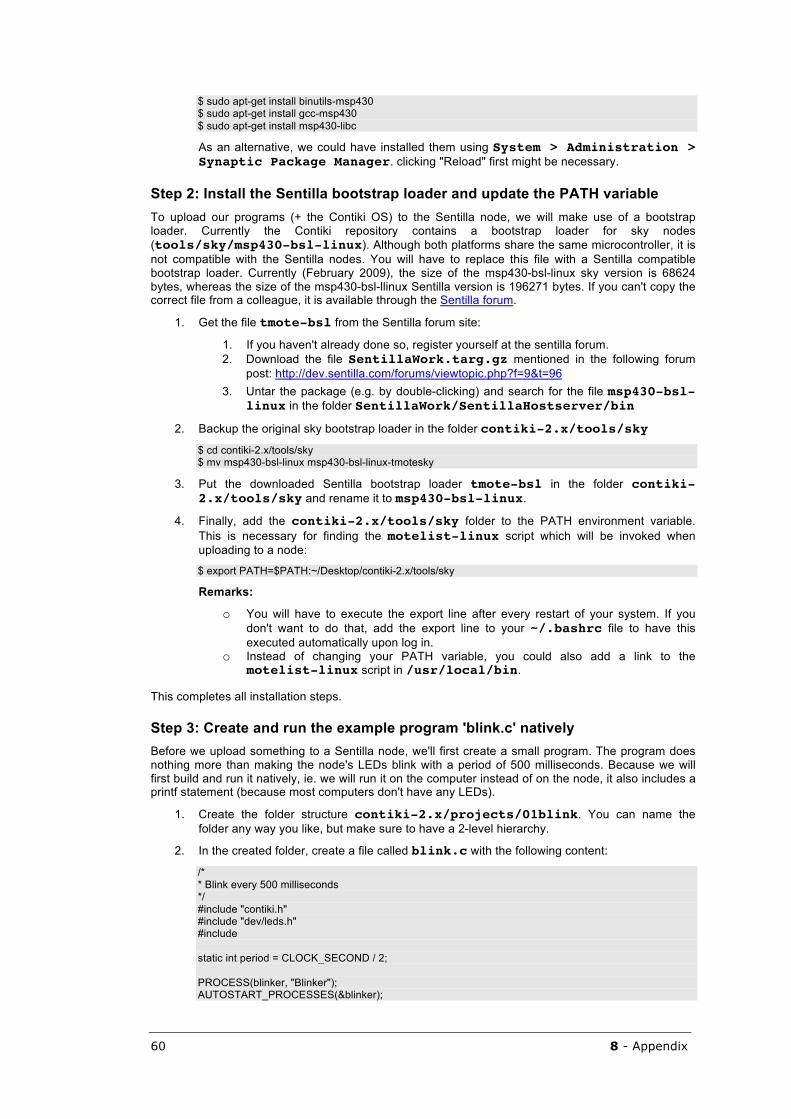
60 8 - Appendix
$ sudo apt-get install binutils-msp430 $ sudo apt-get install gcc-msp430 $ sudo apt-get install msp430-libc
As an alternative, we could have installed them using System > Administration > Synaptic Package Manager. clicking "Reload" first might be necessary.
Step 2: Install the Sentilla bootstrap loader and update the PATH variable To upload our programs (+ the Contiki OS) to the Sentilla node, we will make use of a bootstrap loader. Currently the Contiki repository contains a bootstrap loader for sky nodes (tools/sky/msp430-bsl-linux). Although both platforms share the same microcontroller, it is not compatible with the Sentilla nodes. You will have to replace this file with a Sentilla compatible bootstrap loader. Currently (February 2009), the size of the msp430-bsl-linux sky version is 68624 bytes, whereas the size of the msp430-bsl-llinux Sentilla version is 196271 bytes. If you can't copy the correct file from a colleague, it is available through the Sentilla forum.
1. Get the file tmote-bsl from the Sentilla forum site:
1. If you haven't already done so, register yourself at the sentilla forum. 2. Download the file SentillaWork.targ.gz mentioned in the following forum
post: http://dev.sentilla.com/forums/viewtopic.php?f=9&t=96 3. Untar the package (e.g. by double-clicking) and search for the file msp430-bsl-
linux in the folder SentillaWork/SentillaHostserver/bin
2. Backup the original sky bootstrap loader in the folder contiki-2.x/tools/sky
$ cd contiki-2.x/tools/sky $ mv msp430-bsl-linux msp430-bsl-linux-tmotesky
3. Put the downloaded Sentilla bootstrap loader tmote-bsl in the folder contiki-2.x/tools/sky and rename it to msp430-bsl-linux.
4. Finally, add the contiki-2.x/tools/sky folder to the PATH environment variable. This is necessary for finding the motelist-linux script which will be invoked when uploading to a node:
$ export PATH=$PATH:~/Desktop/contiki-2.x/tools/sky
Remarks:
o You will have to execute the export line after every restart of your system. If you don't want to do that, add the export line to your ~/.bashrc file to have this executed automatically upon log in.
o Instead of changing your PATH variable, you could also add a link to the motelist-linux script in /usr/local/bin.
This completes all installation steps.
Step 3: Create and run the example program 'blink.c' natively Before we upload something to a Sentilla node, we'll first create a small program. The program does nothing more than making the node's LEDs blink with a period of 500 milliseconds. Because we will first build and run it natively, ie. we will run it on the computer instead of on the node, it also includes a printf statement (because most computers don't have any LEDs).
1. Create the folder structure contiki-2.x/projects/01blink. You can name the folder any way you like, but make sure to have a 2-level hierarchy.
2. In the created folder, create a file called blink.c with the following content:
/* * Blink every 500 milliseconds */ #include "contiki.h" #include "dev/leds.h" #include static int period = CLOCK_SECOND / 2; PROCESS(blinker, "Blinker"); AUTOSTART_PROCESSES(&blinker);
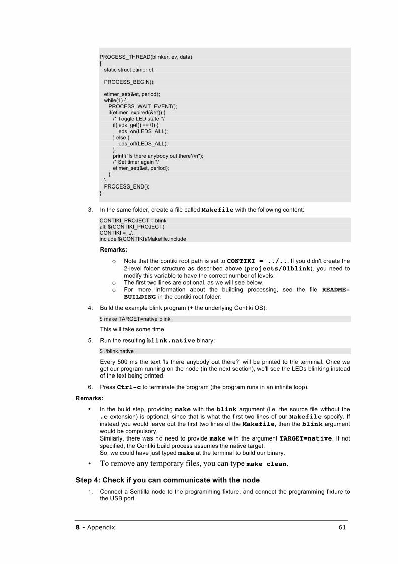
8 - Appendix 61
PROCESS_THREAD(blinker, ev, data) { static struct etimer et; PROCESS_BEGIN(); etimer_set(&et, period); while(1) { PROCESS_WAIT_EVENT(); if(etimer_expired(&et)) { /* Toggle LED state */ if(leds_get() == 0) { leds_on(LEDS_ALL); } else { leds_off(LEDS_ALL); } printf("Is there anybody out there?\n"); /* Set timer again */ etimer_set(&et, period); } } PROCESS_END(); }
3. In the same folder, create a file called Makefile with the following content:
CONTIKI_PROJECT = blink all: $(CONTIKI_PROJECT) CONTIKI = ../.. include $(CONTIKI)/Makefile.include
Remarks:
o Note that the contiki root path is set to CONTIKI = ../... If you didn't create the 2-level folder structure as described above (projects/01blink), you need to modify this variable to have the correct number of levels.
o The first two lines are optional, as we will see below. o For more information about the building processing, see the file README-
BUILDING in the contiki root folder.
4. Build the example blink program (+ the underlying Contiki OS):
$ make TARGET=native blink
This will take some time.
5. Run the resulting blink.native binary:
$ ./blink.native
Every 500 ms the text 'Is there anybody out there?' will be printed to the terminal. Once we get our program running on the node (in the next section), we'll see the LEDs blinking instead of the text being printed.
6. Press Ctrl-c to terminate the program (the program runs in an infinite loop).
Remarks:
• In the build step, providing make with the blink argument (i.e. the source file without the .c extension) is optional, since that is what the first two lines of our Makefile specify. If instead you would leave out the first two lines of the Makefile, then the blink argument would be compulsory. Similarly, there was no need to provide make with the argument TARGET=native. If not specified, the Contiki build process assumes the native target. So, we could have just typed make at the terminal to build our binary.
• To remove any temporary files, you can type make clean.
Step 4: Check if you can communicate with the node 1. Connect a Sentilla node to the programming fixture, and connect the programming fixture to
the USB port.
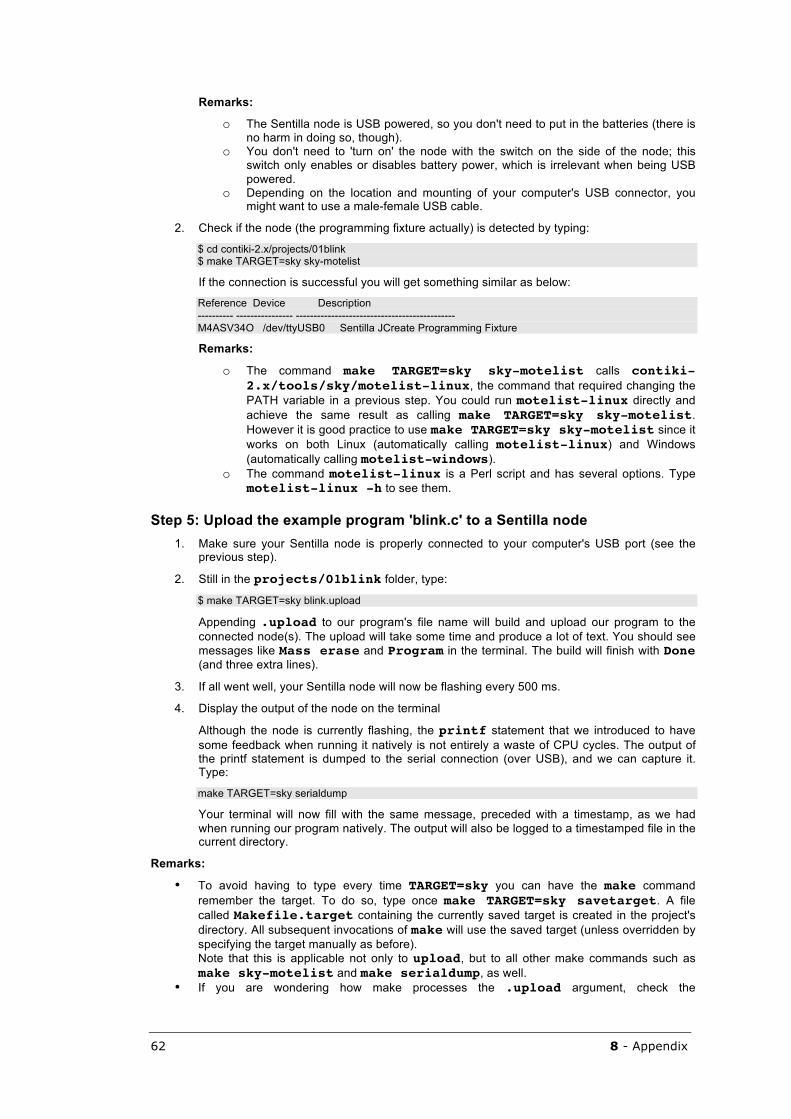
62 8 - Appendix
Remarks:
o The Sentilla node is USB powered, so you don't need to put in the batteries (there is no harm in doing so, though).
o You don't need to 'turn on' the node with the switch on the side of the node; this switch only enables or disables battery power, which is irrelevant when being USB powered.
o Depending on the location and mounting of your computer's USB connector, you might want to use a male-female USB cable.
2. Check if the node (the programming fixture actually) is detected by typing:
$ cd contiki-2.x/projects/01blink $ make TARGET=sky sky-motelist
If the connection is successful you will get something similar as below:
Reference Device Description ---------- ---------------- --------------------------------------------- M4ASV34O /dev/ttyUSB0 Sentilla JCreate Programming Fixture
Remarks:
o The command make TARGET=sky sky-motelist calls contiki-2.x/tools/sky/motelist-linux, the command that required changing the PATH variable in a previous step. You could run motelist-linux directly and achieve the same result as calling make TARGET=sky sky-motelist. However it is good practice to use make TARGET=sky sky-motelist since it works on both Linux (automatically calling motelist-linux) and Windows (automatically calling motelist-windows).
o The command motelist-linux is a Perl script and has several options. Type motelist-linux -h to see them.
Step 5: Upload the example program 'blink.c' to a Sentilla node 1. Make sure your Sentilla node is properly connected to your computer's USB port (see the
previous step).
2. Still in the projects/01blink folder, type:
$ make TARGET=sky blink.upload
Appending .upload to our program's file name will build and upload our program to the connected node(s). The upload will take some time and produce a lot of text. You should see messages like Mass erase and Program in the terminal. The build will finish with Done (and three extra lines).
3. If all went well, your Sentilla node will now be flashing every 500 ms.
4. Display the output of the node on the terminal
Although the node is currently flashing, the printf statement that we introduced to have some feedback when running it natively is not entirely a waste of CPU cycles. The output of the printf statement is dumped to the serial connection (over USB), and we can capture it. Type:
make TARGET=sky serialdump
Your terminal will now fill with the same message, preceded with a timestamp, as we had when running our program natively. The output will also be logged to a timestamped file in the current directory.
Remarks:
• To avoid having to type every time TARGET=sky you can have the make command remember the target. To do so, type once make TARGET=sky savetarget. A file called Makefile.target containing the currently saved target is created in the project's directory. All subsequent invocations of make will use the saved target (unless overridden by specifying the target manually as before). Note that this is applicable not only to upload, but to all other make commands such as make sky-motelist and make serialdump, as well.
• If you are wondering how make processes the .upload argument, check the
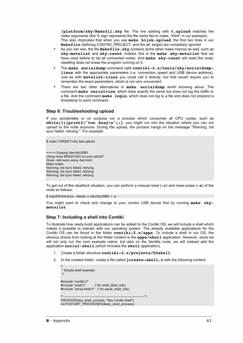
8 - Appendix 63
/platform/sky/Makefil.sky file. The line starting with %.upload matches the make arguments (the % sign represents the file name fed to make, "blink" in our example). This also implicates that when you use make blink.upload, the first two lines in our Makefile (defining CONTIKI_PROJECT, and the all: target) are completely ignored.
• As you can see, the file Makefile.sky contains some other make macros as well, such as sky-motelist and sky-reset. Indeed, this is the make sky-motelist that we have used before to list all connected nodes. And make sky-reset will reset the node; resetting does not erase the program running on it.
• The make serialdump command calls contiki-2.x/tools/sky/serialdump-linux with the appropriate parameters (i.e. connection speed and USB device address). Just as with motelist-linux you could call it directly, but that would require you to remember the exact parameters, which is not very convenient.
• There are two other alternatives to make serialdump worth knowing about. The command make serialview, which does exactly the same but does not log the traffic to a file. And the command make login, which does not log to a file and does not prepend a timestamp to each command.
Step 6: Troubleshooting upload If you accidentally or on purpose run a process which consumes all CPU cycles, such as while(1){printf("too busy\n");}, you might run into the situation where you can not upload to the node anymore. During the upload, the process hangs on the message "Warning, bsl sync failed, retrying.". For example:
$ make TARGET=sky test.upload ... +++++ Erasing /dev/ttyUSB0 Using mote M4ASV34O on port usb2d7. Given -bsl=auto using -bsl=mini Mass erase. Warning, bsl sync failed, retrying. Warning, bsl sync failed, retrying. Warning, bsl sync failed, retrying. ...
To get out of this deadlock situation, you can perform a manual reset (-r) and mass erase (-e) of the node as follows:
$ msp430-bsl-linux --telosb -c /dev/ttyUSB0 -r -e
You might want to check and change to your correct USB device first by running make sky-motelist.
Step 7: Including a shell into Contiki To illustrate how ready-build applications can be added to the Contiki OS, we will include a shell which makes it possible to interact with our operating system. The already available applications for the Contiki OS can be found in the folder contiki-2.x/apps. To include a shell in our OS, the obvious choice from looking at the folder content is the apps/shell application. However, since we will not only run the next example native, but also on the Sentilla node, we will instead add the application serial-shell (which includes the shell application).
1. Create a folder structure contiki-2.x/projects/02shell.
2. In the created folder, create a file called jcreate-shell.c with the following content:
/* * Simple shell example */ #include "contiki.h" #include "shell.h" // for shell_blink_init() #include "serial-shell.h" // for serial_shell_init() /*---------------------------------------------------------------------------*/ PROCESS(sky_shell_process, "Sky Contiki shell"); AUTOSTART_PROCESSES(&sky_shell_process);
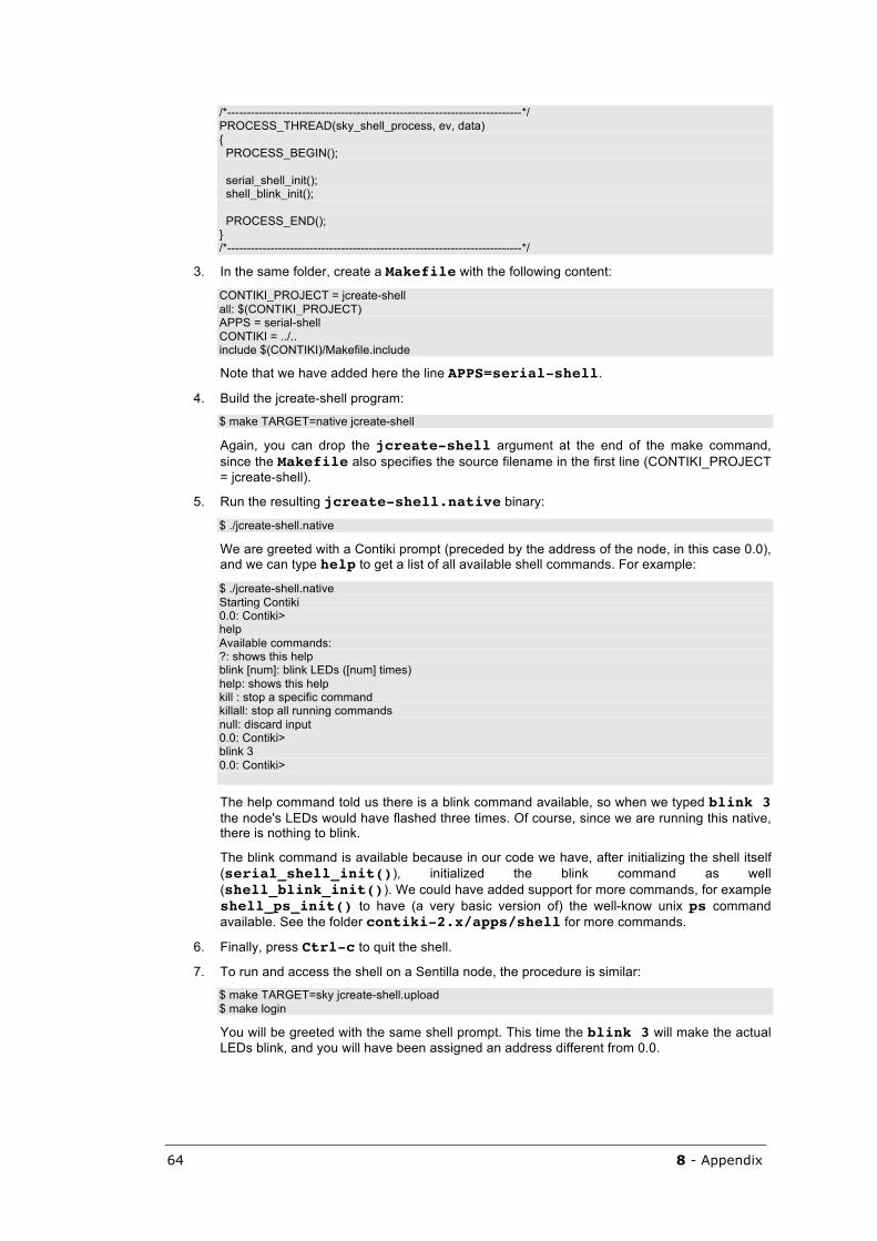
64 8 - Appendix
/*---------------------------------------------------------------------------*/ PROCESS_THREAD(sky_shell_process, ev, data) { PROCESS_BEGIN(); serial_shell_init(); shell_blink_init(); PROCESS_END(); } /*---------------------------------------------------------------------------*/
3. In the same folder, create a Makefile with the following content:
CONTIKI_PROJECT = jcreate-shell all: $(CONTIKI_PROJECT) APPS = serial-shell CONTIKI = ../.. include $(CONTIKI)/Makefile.include
Note that we have added here the line APPS=serial-shell.
4. Build the jcreate-shell program:
$ make TARGET=native jcreate-shell
Again, you can drop the jcreate-shell argument at the end of the make command, since the Makefile also specifies the source filename in the first line (CONTIKI_PROJECT = jcreate-shell).
5. Run the resulting jcreate-shell.native binary:
$ ./jcreate-shell.native
We are greeted with a Contiki prompt (preceded by the address of the node, in this case 0.0), and we can type help to get a list of all available shell commands. For example:
$ ./jcreate-shell.native Starting Contiki 0.0: Contiki> help Available commands: ?: shows this help blink [num]: blink LEDs ([num] times) help: shows this help kill : stop a specific command killall: stop all running commands null: discard input 0.0: Contiki> blink 3 0.0: Contiki>
The help command told us there is a blink command available, so when we typed blink 3 the node's LEDs would have flashed three times. Of course, since we are running this native, there is nothing to blink.
The blink command is available because in our code we have, after initializing the shell itself (serial_shell_init()), initialized the blink command as well (shell_blink_init()). We could have added support for more commands, for example shell_ps_init() to have (a very basic version of) the well-know unix ps command available. See the folder contiki-2.x/apps/shell for more commands.
6. Finally, press Ctrl-c to quit the shell.
7. To run and access the shell on a Sentilla node, the procedure is similar:
$ make TARGET=sky jcreate-shell.upload $ make login
You will be greeted with the same shell prompt. This time the blink 3 will make the actual LEDs blink, and you will have been assigned an address different from 0.0.
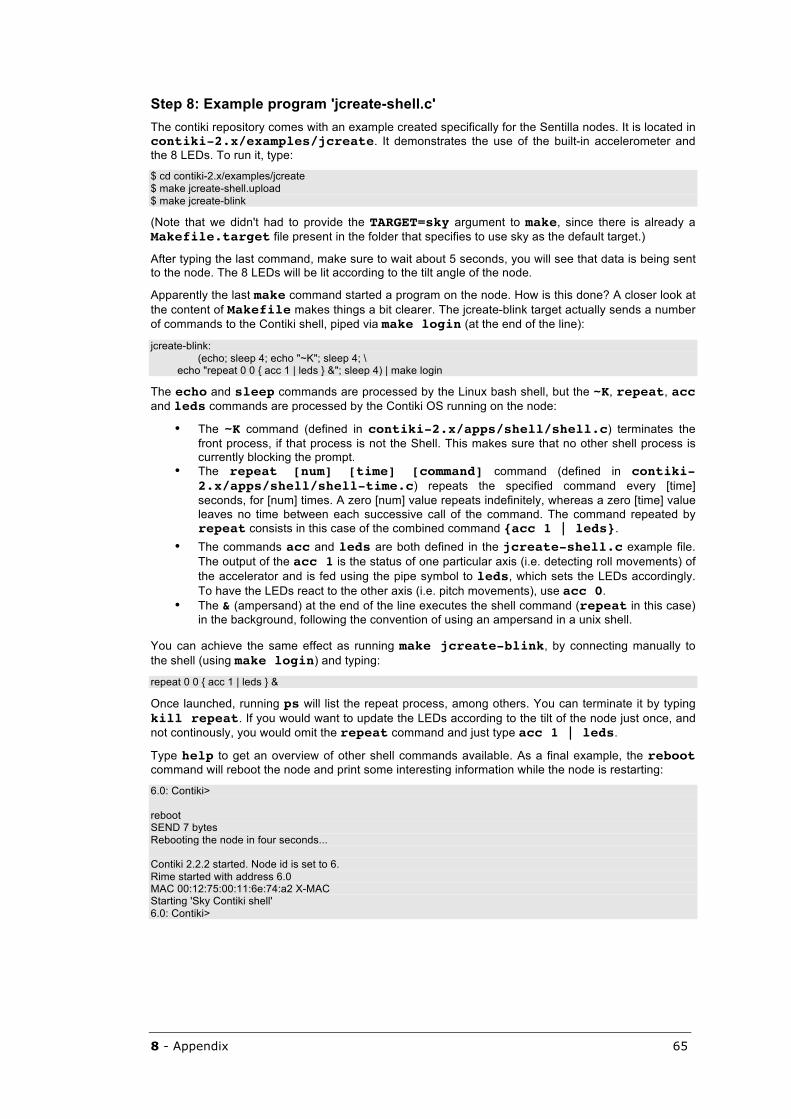
8 - Appendix 65
Step 8: Example program 'jcreate-shell.c' The contiki repository comes with an example created specifically for the Sentilla nodes. It is located in contiki-2.x/examples/jcreate. It demonstrates the use of the built-in accelerometer and the 8 LEDs. To run it, type:
$ cd contiki-2.x/examples/jcreate $ make jcreate-shell.upload $ make jcreate-blink
(Note that we didn't had to provide the TARGET=sky argument to make, since there is already a Makefile.target file present in the folder that specifies to use sky as the default target.)
After typing the last command, make sure to wait about 5 seconds, you will see that data is being sent to the node. The 8 LEDs will be lit according to the tilt angle of the node.
Apparently the last make command started a program on the node. How is this done? A closer look at the content of Makefile makes things a bit clearer. The jcreate-blink target actually sends a number of commands to the Contiki shell, piped via make login (at the end of the line):
jcreate-blink: (echo; sleep 4; echo "~K"; sleep 4; \ echo "repeat 0 0 { acc 1 | leds } &"; sleep 4) | make login
The echo and sleep commands are processed by the Linux bash shell, but the ~K, repeat, acc and leds commands are processed by the Contiki OS running on the node:
• The ~K command (defined in contiki-2.x/apps/shell/shell.c) terminates the front process, if that process is not the Shell. This makes sure that no other shell process is currently blocking the prompt.
• The repeat [num] [time] [command] command (defined in contiki-2.x/apps/shell/shell-time.c) repeats the specified command every [time] seconds, for [num] times. A zero [num] value repeats indefinitely, whereas a zero [time] value leaves no time between each successive call of the command. The command repeated by repeat consists in this case of the combined command {acc 1 | leds}.
• The commands acc and leds are both defined in the jcreate-shell.c example file. The output of the acc 1 is the status of one particular axis (i.e. detecting roll movements) of the accelerator and is fed using the pipe symbol to leds, which sets the LEDs accordingly. To have the LEDs react to the other axis (i.e. pitch movements), use acc 0.
• The & (ampersand) at the end of the line executes the shell command (repeat in this case) in the background, following the convention of using an ampersand in a unix shell.
You can achieve the same effect as running make jcreate-blink, by connecting manually to the shell (using make login) and typing:
repeat 0 0 { acc 1 | leds } &
Once launched, running ps will list the repeat process, among others. You can terminate it by typing kill repeat. If you would want to update the LEDs according to the tilt of the node just once, and not continously, you would omit the repeat command and just type acc 1 | leds.
Type help to get an overview of other shell commands available. As a final example, the reboot command will reboot the node and print some interesting information while the node is restarting:
6.0: Contiki> reboot SEND 7 bytes Rebooting the node in four seconds... Contiki 2.2.2 started. Node id is set to 6. Rime started with address 6.0 MAC 00:12:75:00:11:6e:74:a2 X-MAC Starting 'Sky Contiki shell' 6.0: Contiki>
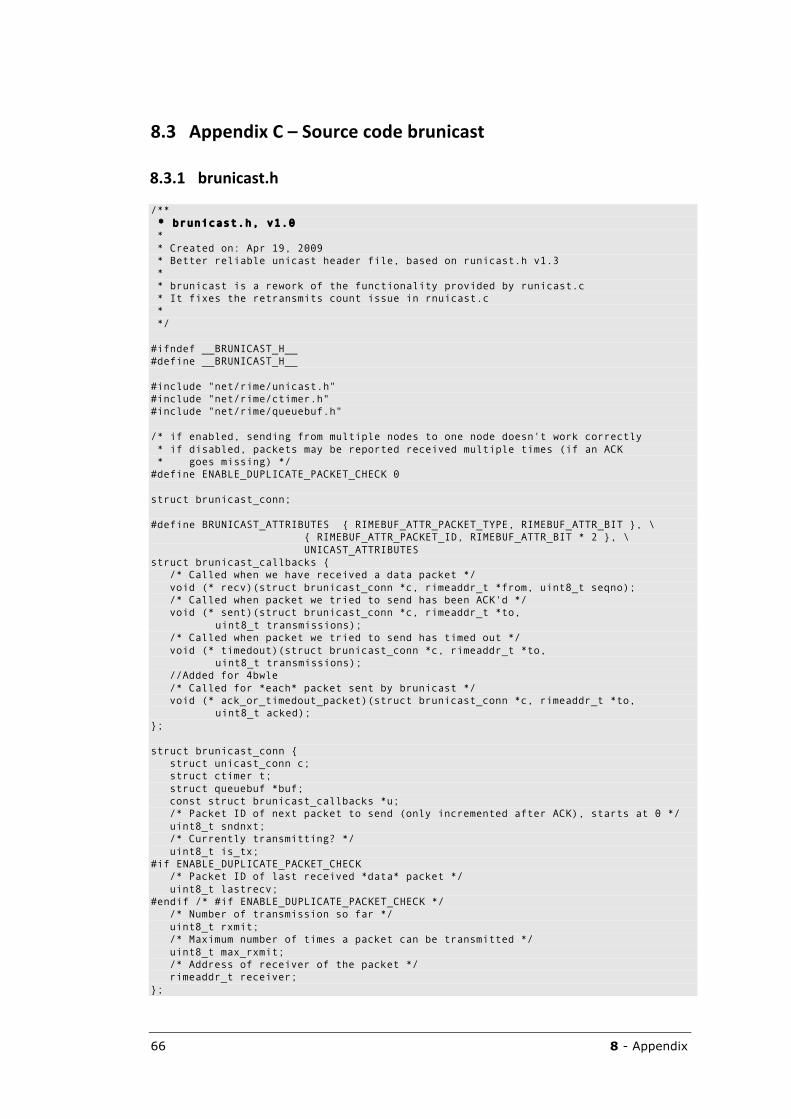
66 8 - Appendix
8.3 AppendixC–Sourcecodebrunicast
8.3.1 brunicast.h
/** * brunicast.h, v1.0 * * Created on: Apr 19, 2009 * Better reliable unicast header file, based on runicast.h v1.3 * * brunicast is a rework of the functionality provided by runicast.c * It fixes the retransmits count issue in rnuicast.c * */ #ifndef __BRUNICAST_H__ #define __BRUNICAST_H__ #include "net/rime/unicast.h" #include "net/rime/ctimer.h" #include "net/rime/queuebuf.h" /* if enabled, sending from multiple nodes to one node doesn't work correctly * if disabled, packets may be reported received multiple times (if an ACK * goes missing) */ #define ENABLE_DUPLICATE_PACKET_CHECK 0 struct brunicast_conn; #define BRUNICAST_ATTRIBUTES { RIMEBUF_ATTR_PACKET_TYPE, RIMEBUF_ATTR_BIT }, \ { RIMEBUF_ATTR_PACKET_ID, RIMEBUF_ATTR_BIT * 2 }, \ UNICAST_ATTRIBUTES struct brunicast_callbacks { /* Called when we have received a data packet */ void (* recv)(struct brunicast_conn *c, rimeaddr_t *from, uint8_t seqno); /* Called when packet we tried to send has been ACK'd */ void (* sent)(struct brunicast_conn *c, rimeaddr_t *to, uint8_t transmissions); /* Called when packet we tried to send has timed out */ void (* timedout)(struct brunicast_conn *c, rimeaddr_t *to, uint8_t transmissions); //Added for 4bwle /* Called for *each* packet sent by brunicast */ void (* ack_or_timedout_packet)(struct brunicast_conn *c, rimeaddr_t *to, uint8_t acked); }; struct brunicast_conn { struct unicast_conn c; struct ctimer t; struct queuebuf *buf; const struct brunicast_callbacks *u; /* Packet ID of next packet to send (only incremented after ACK), starts at 0 */ uint8_t sndnxt; /* Currently transmitting? */ uint8_t is_tx; #if ENABLE_DUPLICATE_PACKET_CHECK /* Packet ID of last received *data* packet */ uint8_t lastrecv; #endif /* #if ENABLE_DUPLICATE_PACKET_CHECK */ /* Number of transmission so far */ uint8_t rxmit; /* Maximum number of times a packet can be transmitted */ uint8_t max_rxmit; /* Address of receiver of the packet */ rimeaddr_t receiver; };
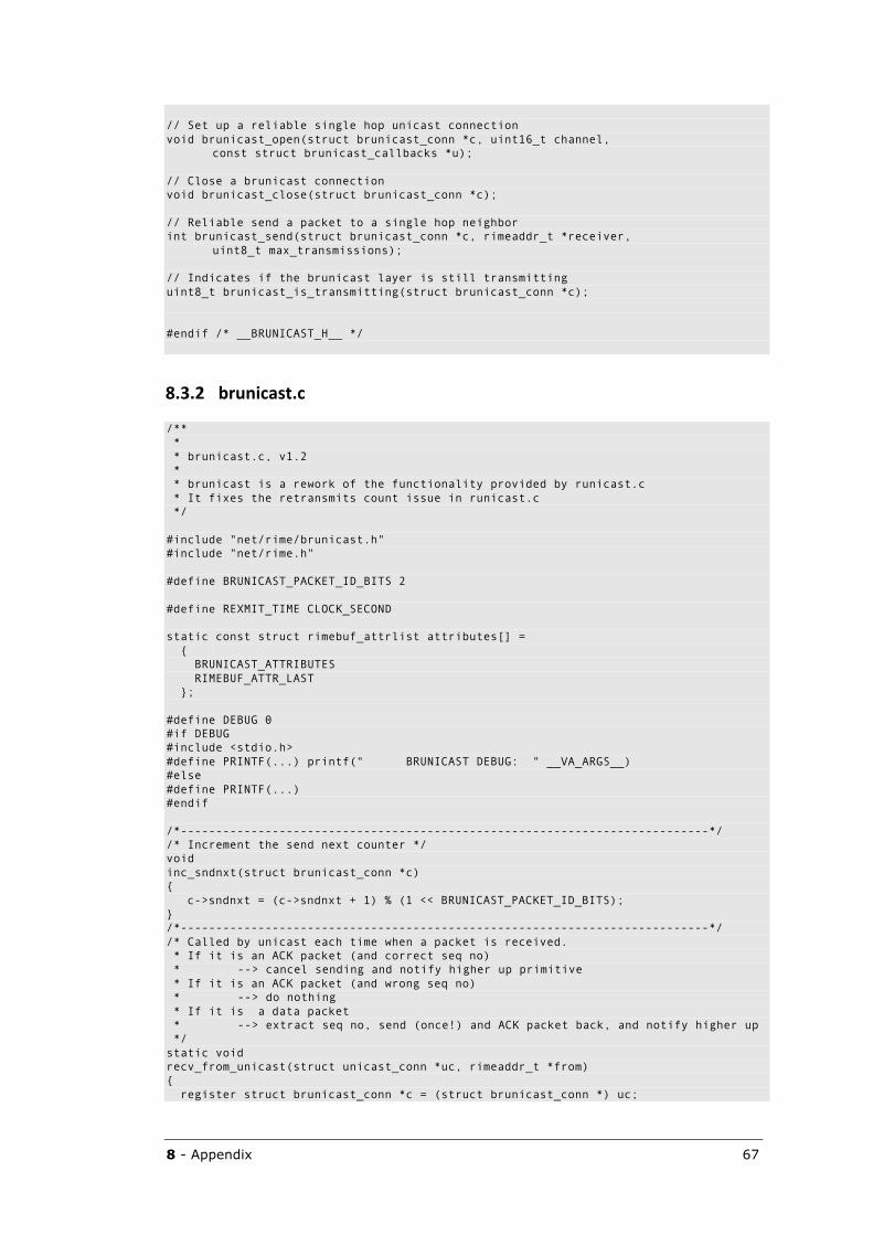
8 - Appendix 67
// Set up a reliable single hop unicast connection void brunicast_open(struct brunicast_conn *c, uint16_t channel, const struct brunicast_callbacks *u); // Close a brunicast connection void brunicast_close(struct brunicast_conn *c); // Reliable send a packet to a single hop neighbor int brunicast_send(struct brunicast_conn *c, rimeaddr_t *receiver, uint8_t max_transmissions); // Indicates if the brunicast layer is still transmitting uint8_t brunicast_is_transmitting(struct brunicast_conn *c); #endif /* __BRUNICAST_H__ */
8.3.2 brunicast.c
/** * * brunicast.c, v1.2 * * brunicast is a rework of the functionality provided by runicast.c * It fixes the retransmits count issue in runicast.c */ #include "net/rime/brunicast.h" #include "net/rime.h" #define BRUNICAST_PACKET_ID_BITS 2 #define REXMIT_TIME CLOCK_SECOND static const struct rimebuf_attrlist attributes[] = { BRUNICAST_ATTRIBUTES RIMEBUF_ATTR_LAST }; #define DEBUG 0 #if DEBUG #include <stdio.h> #define PRINTF(...) printf(" BRUNICAST DEBUG: " __VA_ARGS__) #else #define PRINTF(...) #endif /*---------------------------------------------------------------------------*/ /* Increment the send next counter */ void inc_sndnxt(struct brunicast_conn *c) { c->sndnxt = (c->sndnxt + 1) % (1 << BRUNICAST_PACKET_ID_BITS); } /*---------------------------------------------------------------------------*/ /* Called by unicast each time when a packet is received. * If it is an ACK packet (and correct seq no) * --> cancel sending and notify higher up primitive * If it is an ACK packet (and wrong seq no) * --> do nothing * If it is a data packet * --> extract seq no, send (once!) and ACK packet back, and notify higher up */ static void recv_from_unicast(struct unicast_conn *uc, rimeaddr_t *from) { register struct brunicast_conn *c = (struct brunicast_conn *) uc;
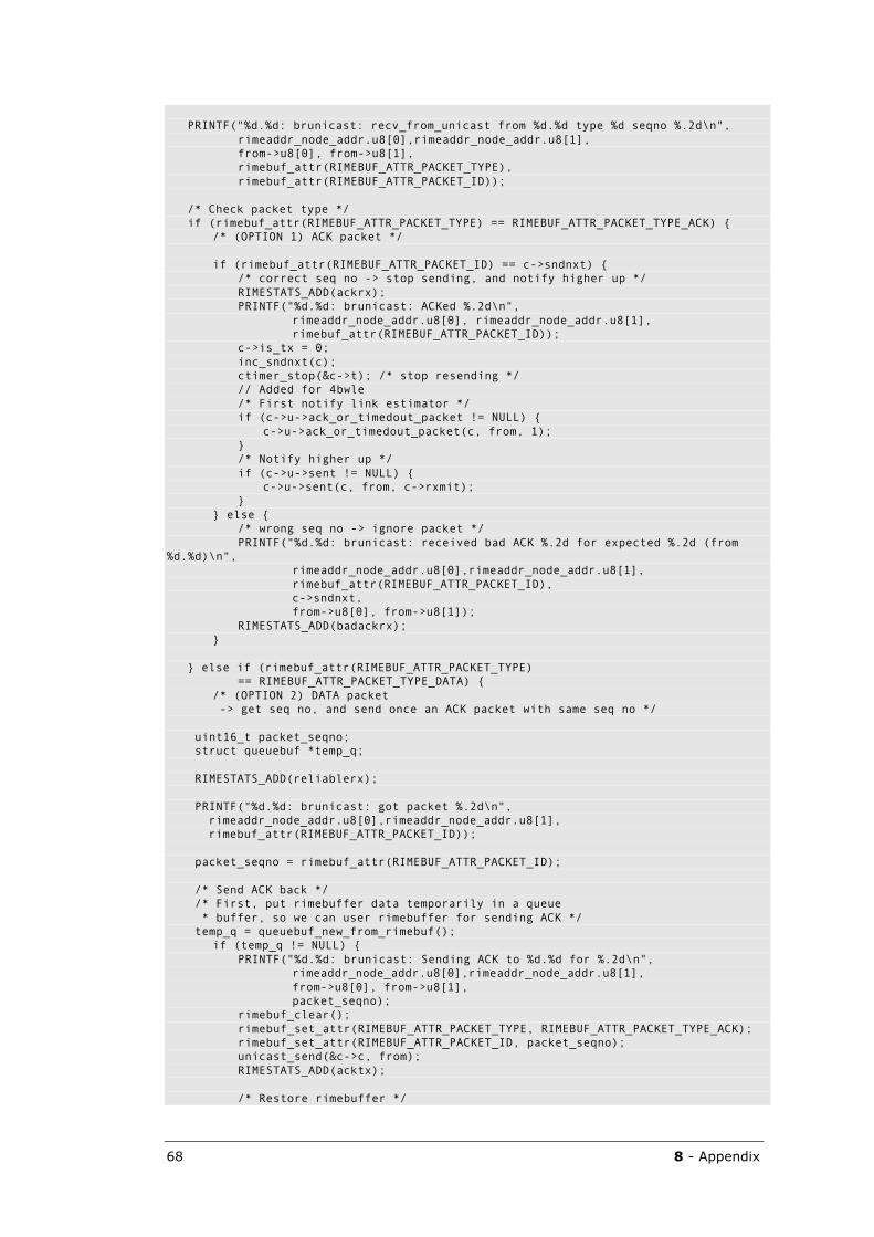
68 8 - Appendix
PRINTF("%d.%d: brunicast: recv_from_unicast from %d.%d type %d seqno %.2d\n", rimeaddr_node_addr.u8[0],rimeaddr_node_addr.u8[1], from->u8[0], from->u8[1], rimebuf_attr(RIMEBUF_ATTR_PACKET_TYPE), rimebuf_attr(RIMEBUF_ATTR_PACKET_ID)); /* Check packet type */ if (rimebuf_attr(RIMEBUF_ATTR_PACKET_TYPE) == RIMEBUF_ATTR_PACKET_TYPE_ACK) { /* (OPTION 1) ACK packet */ if (rimebuf_attr(RIMEBUF_ATTR_PACKET_ID) == c->sndnxt) { /* correct seq no -> stop sending, and notify higher up */ RIMESTATS_ADD(ackrx); PRINTF("%d.%d: brunicast: ACKed %.2d\n", rimeaddr_node_addr.u8[0], rimeaddr_node_addr.u8[1], rimebuf_attr(RIMEBUF_ATTR_PACKET_ID)); c->is_tx = 0; inc_sndnxt(c); ctimer_stop(&c->t); /* stop resending */ // Added for 4bwle /* First notify link estimator */ if (c->u->ack_or_timedout_packet != NULL) { c->u->ack_or_timedout_packet(c, from, 1); } /* Notify higher up */ if (c->u->sent != NULL) { c->u->sent(c, from, c->rxmit); } } else { /* wrong seq no -> ignore packet */ PRINTF("%d.%d: brunicast: received bad ACK %.2d for expected %.2d (from %d.%d)\n", rimeaddr_node_addr.u8[0],rimeaddr_node_addr.u8[1], rimebuf_attr(RIMEBUF_ATTR_PACKET_ID), c->sndnxt, from->u8[0], from->u8[1]); RIMESTATS_ADD(badackrx); } } else if (rimebuf_attr(RIMEBUF_ATTR_PACKET_TYPE) == RIMEBUF_ATTR_PACKET_TYPE_DATA) { /* (OPTION 2) DATA packet -> get seq no, and send once an ACK packet with same seq no */ uint16_t packet_seqno; struct queuebuf *temp_q; RIMESTATS_ADD(reliablerx); PRINTF("%d.%d: brunicast: got packet %.2d\n", rimeaddr_node_addr.u8[0],rimeaddr_node_addr.u8[1], rimebuf_attr(RIMEBUF_ATTR_PACKET_ID)); packet_seqno = rimebuf_attr(RIMEBUF_ATTR_PACKET_ID); /* Send ACK back */ /* First, put rimebuffer data temporarily in a queue * buffer, so we can user rimebuffer for sending ACK */ temp_q = queuebuf_new_from_rimebuf(); if (temp_q != NULL) { PRINTF("%d.%d: brunicast: Sending ACK to %d.%d for %.2d\n", rimeaddr_node_addr.u8[0],rimeaddr_node_addr.u8[1], from->u8[0], from->u8[1], packet_seqno); rimebuf_clear(); rimebuf_set_attr(RIMEBUF_ATTR_PACKET_TYPE, RIMEBUF_ATTR_PACKET_TYPE_ACK); rimebuf_set_attr(RIMEBUF_ATTR_PACKET_ID, packet_seqno); unicast_send(&c->c, from); RIMESTATS_ADD(acktx); /* Restore rimebuffer */
8 - Appendix 69
queuebuf_to_rimebuf(temp_q); queuebuf_free(temp_q); } /* notify higher up about data packet * (duplicate packet dropping disabled to allow multiple nodes to send * to a single node) */ if (c->u->recv != NULL) { #if ENABLE_DUPLICATE_PACKET_CHECK if (packet_seqno != c->lastrecv) { c->u->recv(c, from, packet_seqno); c->lastrecv = packet_seqno; /* remember last received packet */ } else { PRINTF("%d.%d: brunicast: Supressing duplicate receive " "callback from %d.%d for %.2d\n", rimeaddr_node_addr.u8[0],rimeaddr_node_addr.u8[1], from->u8[0], from->u8[1], packet_seqno); } #else c->u->recv(c, from, packet_seqno); #endif /* ENABLE_DUPLICATE_PACKET_CHECK */ } } } /*---------------------------------------------------------------------------*/ /* Send the data in the queuebuffer using unicast */ int send(struct brunicast_conn *c) { queuebuf_to_rimebuf(c->buf); /* get data from queuebuffer */ PRINTF("%d.%d: brunicast send a packet to %d.%d using unicast\n", rimeaddr_node_addr.u8[0],rimeaddr_node_addr.u8[1], c->receiver.u8[0],c->receiver.u8[1]); return unicast_send(&c->c, &c->receiver); } /*---------------------------------------------------------------------------*/ /* Called each time the resend interval has elapsed. * If this gets called, it means we didn't receive an ACK yet * (because an ACK cancels the timer that calls this function). * So, either retransmit the packet or time-out: * - If the maximum number of resends has been reached, time out and notify * higher up. * - Otherwise, resend the packet and double evaluation timer (with a maximum * of 16x the original interval). */ static void evaluate(void *ptr) { struct brunicast_conn *c = ptr; PRINTF("%d.%d: brunicast: evaluating \n", rimeaddr_node_addr.u8[0], rimeaddr_node_addr.u8[1]); /* Check if timed out */ if (c->rxmit >= c->max_rxmit) { /* timed out */ RIMESTATS_ADD(timedout); PRINTF("%d.%d: brunicast: packet %.2d timed out\n", rimeaddr_node_addr.u8[0],rimeaddr_node_addr.u8[1], c->sndnxt); c->is_tx = 0; inc_sndnxt(c); // TODO better to free queuebuffer here? (otherwise, this will only // be done when/if a new packet is sent) // added for 4bwle /* First notify link estimator */ if (c->u->ack_or_timedout_packet != NULL) { c->u->ack_or_timedout_packet(c, &c->receiver, 0); } /* notify higher up */ if (c->u->timedout) { c->u->timedout(c, &c->receiver, c->rxmit);
70 8 - Appendix
} } else { /* rexmit time has elapsed (and not reach maximum resends * -> resend (with increasing interval)*/ c->rxmit++; RIMESTATS_ADD(rexmit); PRINTF("%d.%d: brunicast: packet %.2d resent %u\n", rimeaddr_node_addr.u8[0], rimeaddr_node_addr.u8[1], c->sndnxt, c->rxmit); // Added for 4bwle /* First notify link estimator */ if (c->u->ack_or_timedout_packet != NULL) { c->u->ack_or_timedout_packet(c, &c->receiver, 0); } /* send packet */ send(c); /* set timer */ int shift; shift = c->rxmit > 4 ? 4 : (c->rxmit-1); //2 x interval (and maximum 16x) ctimer_set(&c->t, (REXMIT_TIME) << shift, evaluate, c); PRINTF("%d.%d: brunicast: next send timer set to %d seconds.\n", rimeaddr_node_addr.u8[0], rimeaddr_node_addr.u8[1], ((REXMIT_TIME)<<shift)/CLOCK_SECOND); } } /*---------------------------------------------------------------------------*/ static const struct unicast_callbacks brunicast = {recv_from_unicast}; /*---------------------------------------------------------------------------*/ void brunicast_open(struct brunicast_conn *c, uint16_t channel, const struct brunicast_callbacks *u) { unicast_open(&c->c, channel, &brunicast); channel_set_attributes(channel, attributes); c->u = u; c->rxmit = 0; c->sndnxt = 0; c->is_tx = 0; #if ENABLE_DUPLICATE_PACKET_CHECK c->lastrecv = 0xFF; #endif /* ENABLE_DUPLICATE_PACKET_CHECK */ } /*---------------------------------------------------------------------------*/ void brunicast_close(struct brunicast_conn *c) { unicast_close(&c->c); ctimer_stop(&c->t); if (c->buf != NULL) { queuebuf_free(c->buf); } } /*---------------------------------------------------------------------------*/ int brunicast_send(struct brunicast_conn *c, rimeaddr_t *receiver, uint8_t max_transmissions) { if (brunicast_is_transmitting(c)) { RIMESTATS_ADD(bruni_tx_busy); PRINTF("%d.%d: brunicast: already transmitting\n", rimeaddr_node_addr.u8[0],rimeaddr_node_addr.u8[1]); return 0; } /* Configure packet attributes and connection parameters */ rimebuf_set_attr(RIMEBUF_ATTR_RELIABLE, 1); rimebuf_set_attr(RIMEBUF_ATTR_PACKET_TYPE, RIMEBUF_ATTR_PACKET_TYPE_DATA); rimebuf_set_attr(RIMEBUF_ATTR_PACKET_ID, c->sndnxt); c->max_rxmit = max_transmissions; rimeaddr_copy(&c->receiver, receiver);
8 - Appendix 71
/* Put data in a queue buffer */ if (c->buf != NULL) { queuebuf_free(c->buf); } c->buf = queuebuf_new_from_rimebuf(); if (c->buf == NULL) { return 0; } RIMESTATS_ADD(reliabletx); PRINTF("%d.%d: brunicast: sending packet %.2d\n", rimeaddr_node_addr.u8[0],rimeaddr_node_addr.u8[1], c->sndnxt); /* Send */ c->is_tx = 1; c->rxmit = 1; int result; result = send(c); ctimer_set(&c->t, REXMIT_TIME, evaluate, c); return result; } /*---------------------------------------------------------------------------*/ uint8_t brunicast_is_transmitting(struct brunicast_conn *c) { return c->is_tx; } /*---------------------------------------------------------------------------*/
72 8 - Appendix
8.4 AppendixD–Sourcecode4B
8.4.1 neighbor.h
/** * neighbor.h * The neighbor module manages the neighbor table. */ #ifndef __NEIGHBOR_H__ #define __NEIGHBOR_H__ #include "net/rime/rimeaddr.h" #if USE_4BWLE #include "net/rime/brunicast.h" #include "net/rime/collect.h" // (needed for neighbor_start) #endif /* USE_4BWLE */ #if USE_4BWLE // The etx returned is scaled by this factor. #define NEIGHBOR_ETX_SCALE 10 #else #define NEIGHBOR_ETX_SCALE 10 #define NEIGHBOR_NUM_ETXS 8 //Capacity of etx circular history buffer #endif #if USE_4BWLE struct neighbor { struct neighbor *next; uint16_t time; rimeaddr_t addr; uint16_t rtmetric; /* Beacons */ // last beacon sequence number received from this neighbor uint8_t beac_lastseq; // number of beacons received after last beacon estimator update // the update happens every BLQ_PKT_WINDOW beacon packets uint8_t beac_rcvcnt; // number of beacon packets missed after last beacon estimator update uint8_t beac_failcnt; // Flag to indicate that this link has received the // first sequence number. If 1, the link is initialized (has received a // sequence number) uint8_t beac_init_entry; // MAXAGE-inage gives the number of update rounds we haven't been able // update the inbound beacon estimator // uint8_t beac_inage; //TODO wegdoen (of niet?) // inbound qualities in the range [1..255] // 1 bad, 255 good, 0 indicates pristine state (important for EWMA) uint8_t beac_inquality; /* Data driven */ // Number of data packets successfully sent (ack'd) to this neighbor // since the last data estimator update round. This update happens // every DLQ_PKT_WINDOW data packets uint8_t data_success; // The total number of data packets transmission attempt to this neighbor // since the last data estimator update round. uint8_t data_total; // ETX for the link to this neighbor. This is the quality returned to // the users of the link estimator (scaled) uint16_t etx;
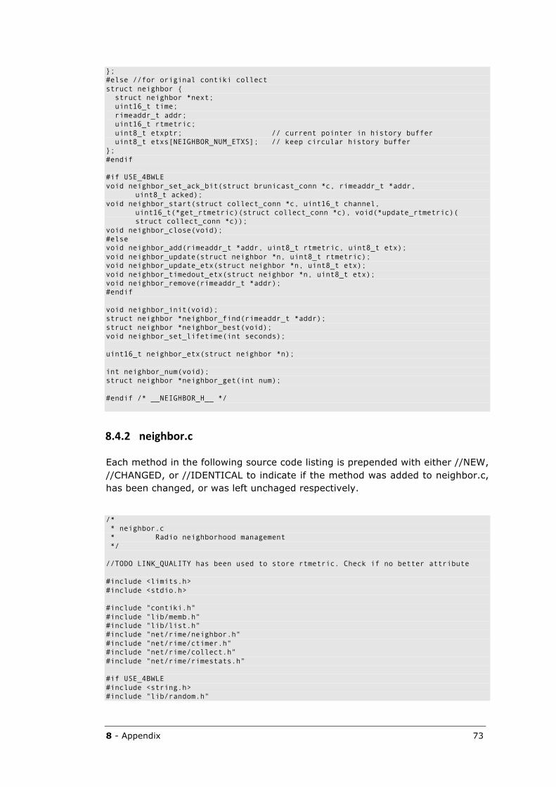
8 - Appendix 73
}; #else //for original contiki collect struct neighbor { struct neighbor *next; uint16_t time; rimeaddr_t addr; uint16_t rtmetric; uint8_t etxptr; // current pointer in history buffer uint8_t etxs[NEIGHBOR_NUM_ETXS]; // keep circular history buffer }; #endif #if USE_4BWLE void neighbor_set_ack_bit(struct brunicast_conn *c, rimeaddr_t *addr, uint8_t acked); void neighbor_start(struct collect_conn *c, uint16_t channel, uint16_t(*get_rtmetric)(struct collect_conn *c), void(*update_rtmetric)( struct collect_conn *c)); void neighbor_close(void); #else void neighbor_add(rimeaddr_t *addr, uint8_t rtmetric, uint8_t etx); void neighbor_update(struct neighbor *n, uint8_t rtmetric); void neighbor_update_etx(struct neighbor *n, uint8_t etx); void neighbor_timedout_etx(struct neighbor *n, uint8_t etx); void neighbor_remove(rimeaddr_t *addr); #endif void neighbor_init(void); struct neighbor *neighbor_find(rimeaddr_t *addr); struct neighbor *neighbor_best(void); void neighbor_set_lifetime(int seconds); uint16_t neighbor_etx(struct neighbor *n); int neighbor_num(void); struct neighbor *neighbor_get(int num); #endif /* __NEIGHBOR_H__ */
8.4.2 neighbor.c
Each method in the following source code listing is prepended with either //NEW, //CHANGED, or //IDENTICAL to indicate if the method was added to neighbor.c, has been changed, or was left unchaged respectively.
/* * neighbor.c * Radio neighborhood management */ //TODO LINK_QUALITY has been used to store rtmetric. Check if no better attribute #include <limits.h> #include <stdio.h> #include "contiki.h" #include "lib/memb.h" #include "lib/list.h" #include "net/rime/neighbor.h" #include "net/rime/ctimer.h" #include "net/rime/collect.h" #include "net/rime/rimestats.h" #if USE_4BWLE #include <string.h> #include "lib/random.h"
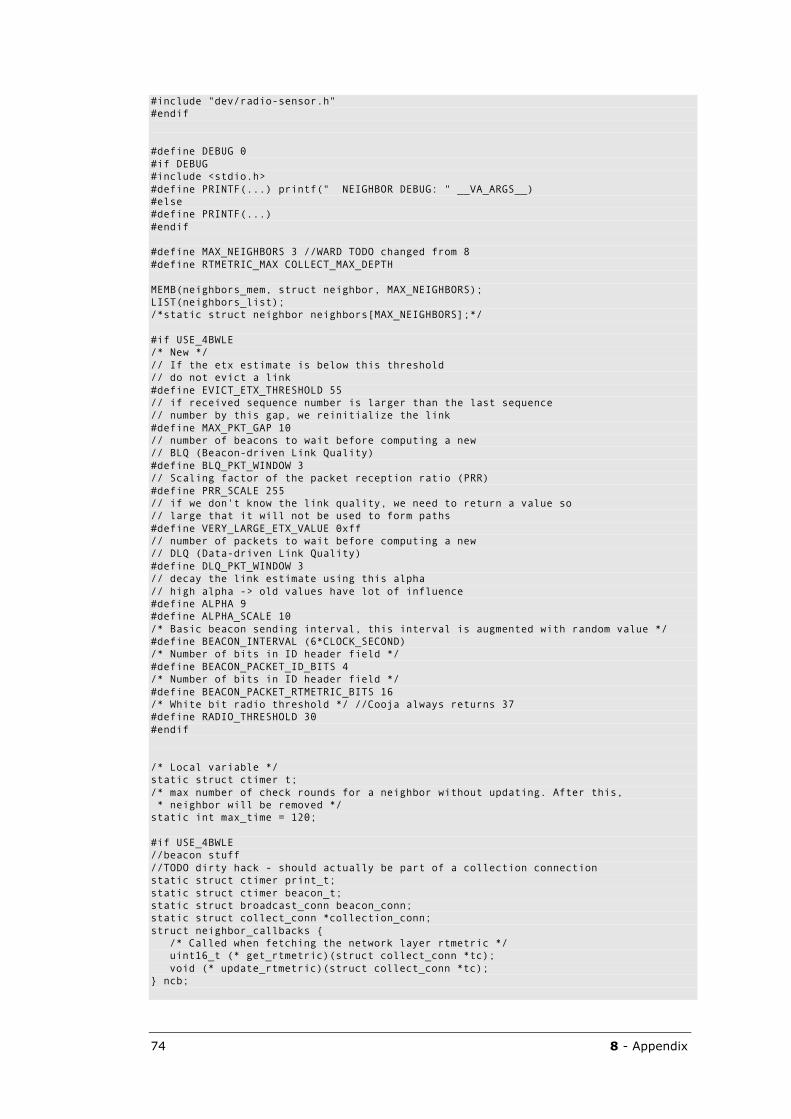
74 8 - Appendix
#include "dev/radio-sensor.h" #endif #define DEBUG 0 #if DEBUG #include <stdio.h> #define PRINTF(...) printf(" NEIGHBOR DEBUG: " __VA_ARGS__) #else #define PRINTF(...) #endif #define MAX_NEIGHBORS 3 //WARD TODO changed from 8 #define RTMETRIC_MAX COLLECT_MAX_DEPTH MEMB(neighbors_mem, struct neighbor, MAX_NEIGHBORS); LIST(neighbors_list); /*static struct neighbor neighbors[MAX_NEIGHBORS];*/ #if USE_4BWLE /* New */ // If the etx estimate is below this threshold // do not evict a link #define EVICT_ETX_THRESHOLD 55 // if received sequence number is larger than the last sequence // number by this gap, we reinitialize the link #define MAX_PKT_GAP 10 // number of beacons to wait before computing a new // BLQ (Beacon-driven Link Quality) #define BLQ_PKT_WINDOW 3 // Scaling factor of the packet reception ratio (PRR) #define PRR_SCALE 255 // if we don't know the link quality, we need to return a value so // large that it will not be used to form paths #define VERY_LARGE_ETX_VALUE 0xff // number of packets to wait before computing a new // DLQ (Data-driven Link Quality) #define DLQ_PKT_WINDOW 3 // decay the link estimate using this alpha // high alpha -> old values have lot of influence #define ALPHA 9 #define ALPHA_SCALE 10 /* Basic beacon sending interval, this interval is augmented with random value */ #define BEACON_INTERVAL (6*CLOCK_SECOND) /* Number of bits in ID header field */ #define BEACON_PACKET_ID_BITS 4 /* Number of bits in ID header field */ #define BEACON_PACKET_RTMETRIC_BITS 16 /* White bit radio threshold */ //Cooja always returns 37 #define RADIO_THRESHOLD 30 #endif /* Local variable */ static struct ctimer t; /* max number of check rounds for a neighbor without updating. After this, * neighbor will be removed */ static int max_time = 120; #if USE_4BWLE //beacon stuff //TODO dirty hack - should actually be part of a collection connection static struct ctimer print_t; static struct ctimer beacon_t; static struct broadcast_conn beacon_conn; static struct collect_conn *collection_conn; struct neighbor_callbacks { /* Called when fetching the network layer rtmetric */ uint16_t (* get_rtmetric)(struct collect_conn *tc); void (* update_rtmetric)(struct collect_conn *tc); } ncb;
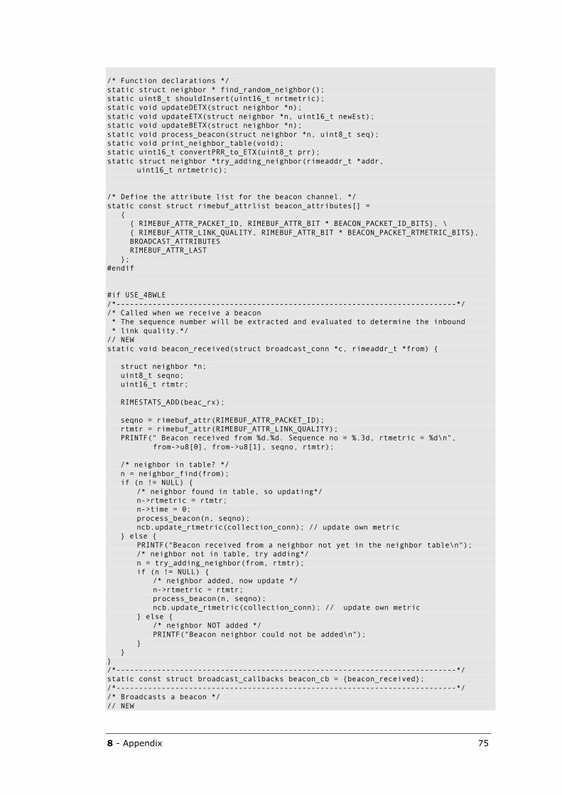
8 - Appendix 75
/* Function declarations */ static struct neighbor * find_random_neighbor(); static uint8_t shouldInsert(uint16_t nrtmetric); static void updateDETX(struct neighbor *n); static void updateETX(struct neighbor *n, uint16_t newEst); static void updateBETX(struct neighbor *n); static void process_beacon(struct neighbor *n, uint8_t seq); static void print_neighbor_table(void); static uint16_t convertPRR_to_ETX(uint8_t prr); static struct neighbor *try_adding_neighbor(rimeaddr_t *addr, uint16_t nrtmetric); /* Define the attribute list for the beacon channel. */ static const struct rimebuf_attrlist beacon_attributes[] = { { RIMEBUF_ATTR_PACKET_ID, RIMEBUF_ATTR_BIT * BEACON_PACKET_ID_BITS}, \ { RIMEBUF_ATTR_LINK_QUALITY, RIMEBUF_ATTR_BIT * BEACON_PACKET_RTMETRIC_BITS}, BROADCAST_ATTRIBUTES RIMEBUF_ATTR_LAST }; #endif #if USE_4BWLE /*---------------------------------------------------------------------------*/ /* Called when we receive a beacon * The sequence number will be extracted and evaluated to determine the inbound * link quality.*/ // NEW static void beacon_received(struct broadcast_conn *c, rimeaddr_t *from) { struct neighbor *n; uint8_t seqno; uint16_t rtmtr; RIMESTATS_ADD(beac_rx); seqno = rimebuf_attr(RIMEBUF_ATTR_PACKET_ID); rtmtr = rimebuf_attr(RIMEBUF_ATTR_LINK_QUALITY); PRINTF(" Beacon received from %d.%d. Sequence no = %.3d, rtmetric = %d\n", from->u8[0], from->u8[1], seqno, rtmtr); /* neighbor in table? */ n = neighbor_find(from); if (n != NULL) { /* neighbor found in table, so updating*/ n->rtmetric = rtmtr; n->time = 0; process_beacon(n, seqno); ncb.update_rtmetric(collection_conn); // update own metric } else { PRINTF("Beacon received from a neighbor not yet in the neighbor table\n"); /* neighbor not in table, try adding*/ n = try_adding_neighbor(from, rtmtr); if (n != NULL) { /* neighbor added, now update */ n->rtmetric = rtmtr; process_beacon(n, seqno); ncb.update_rtmetric(collection_conn); // update own metric } else { /* neighbor NOT added */ PRINTF("Beacon neighbor could not be added\n"); } } } /*---------------------------------------------------------------------------*/ static const struct broadcast_callbacks beacon_cb = {beacon_received}; /*---------------------------------------------------------------------------*/ /* Broadcasts a beacon */ // NEW
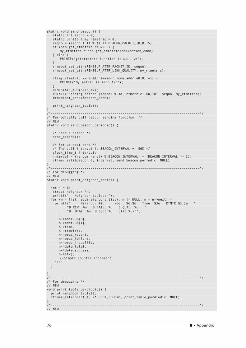
76 8 - Appendix
static void send_beacon() { static int seqno = 0; static uint16_t my_rtmetric = 0; seqno = (seqno + 1) % (1 << BEACON_PACKET_ID_BITS); if (ncb.get_rtmetric != NULL) { my_rtmetric = ncb.get_rtmetric(collection_conn); } else { PRINTF("getrtmetric function is NULL \n"); } rimebuf_set_attr(RIMEBUF_ATTR_PACKET_ID, seqno); rimebuf_set_attr(RIMEBUF_ATTR_LINK_QUALITY, my_rtmetric); if(my_rtmetric == 0 && rimeaddr_node_addr.u8[0]!=1) { PRINTF("My metric is zero !\n"); } RIMESTATS_ADD(beac_tx); PRINTF("Sending beacon (seqno: %.3d, rtmetric: %u)\n", seqno, my_rtmetric); broadcast_send(&beacon_conn); print_neighbor_table(); } /*---------------------------------------------------------------------------*/ /* Periodically call beacon sending function */ // NEW static void send_beacon_periodic() { /* Send a beacon */ send_beacon(); /* Set up next send */ /* The call interval is BEACON_INTERVAL +- 50% */ clock_time_t interval; interval = (random_rand() % BEACON_INTERVAL) + (BEACON_INTERVAL >> 1); ctimer_set(&beacon_t, interval, send_beacon_periodic, NULL); } /*---------------------------------------------------------------------------*/ /* For debugging */ // NEW static void print_neighbor_table() { int i = 0; struct neighbor *n; printf(" Neighbor table:\n"); for (n = list_head(neighbors_list); n != NULL; n = n->next) { printf(" Neighbor %i: addr: %d.%d Time: %3u RTMTR:%3.2u " "B_RCV: %u B_FAIL: %u B_QLT: %u " "D_TOTAL: %u D_SUC: %u ETX: %u\n", i, n->addr.u8[0], n->addr.u8[1], n->time, n->rtmetric, n->beac_rcvcnt, n->beac_failcnt, n->beac_inquality, n->data_total, n->data_success, n->etx); //Simple counter increment i++; } } /*---------------------------------------------------------------------------*/ /* For debugging */ // NEW void print_table_perdiodic() { print_neighbor_table(); ctimer_set(&print_t, 2*CLOCK_SECOND, print_table_perdiodic, NULL); } /*---------------------------------------------------------------------------*/ // NEW
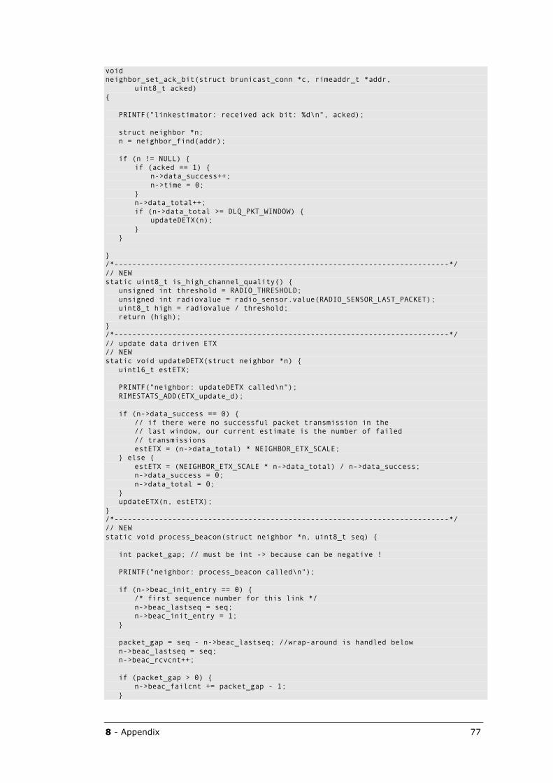
8 - Appendix 77
void neighbor_set_ack_bit(struct brunicast_conn *c, rimeaddr_t *addr, uint8_t acked) { PRINTF("linkestimator: received ack bit: %d\n", acked); struct neighbor *n; n = neighbor_find(addr); if (n != NULL) { if (acked == 1) { n->data_success++; n->time = 0; } n->data_total++; if (n->data_total >= DLQ_PKT_WINDOW) { updateDETX(n); } } } /*---------------------------------------------------------------------------*/ // NEW static uint8_t is_high_channel_quality() { unsigned int threshold = RADIO_THRESHOLD; unsigned int radiovalue = radio_sensor.value(RADIO_SENSOR_LAST_PACKET); uint8_t high = radiovalue / threshold; return (high); } /*---------------------------------------------------------------------------*/ // update data driven ETX // NEW static void updateDETX(struct neighbor *n) { uint16_t estETX; PRINTF("neighbor: updateDETX called\n"); RIMESTATS_ADD(ETX_update_d); if (n->data_success == 0) { // if there were no successful packet transmission in the // last window, our current estimate is the number of failed // transmissions estETX = (n->data_total) * NEIGHBOR_ETX_SCALE; } else { estETX = (NEIGHBOR_ETX_SCALE * n->data_total) / n->data_success; n->data_success = 0; n->data_total = 0; } updateETX(n, estETX); } /*---------------------------------------------------------------------------*/ // NEW static void process_beacon(struct neighbor *n, uint8_t seq) { int packet_gap; // must be int -> because can be negative ! PRINTF("neighbor: process_beacon called\n"); if (n->beac_init_entry == 0) { /* first sequence number for this link */ n->beac_lastseq = seq; n->beac_init_entry = 1; } packet_gap = seq - n->beac_lastseq; //wrap-around is handled below n->beac_lastseq = seq; n->beac_rcvcnt++; if (packet_gap > 0) { n->beac_failcnt += packet_gap - 1; }
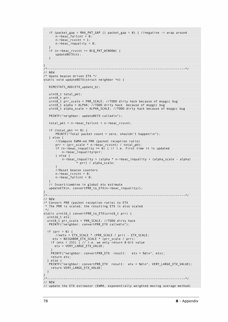
78 8 - Appendix
if (packet_gap > MAX_PKT_GAP || packet_gap < 0) { //negative -> wrap around n->beac_failcnt = 0; n->beac_rcvcnt = 1; n->beac_inquality = 0; } if (n->beac_rcvcnt >= BLQ_PKT_WINDOW) { updateBETX(n); } } /*---------------------------------------------------------------------------*/ // NEW /* Upate beacon driven ETX */ static void updateBETX(struct neighbor *n) { RIMESTATS_ADD(ETX_update_b); uint8_t total_pkt; uint8_t prr; uint8_t prr_scale = PRR_SCALE; //TODO dirty hack because of mspgcc bug uint8_t alpha = ALPHA; //TODO dirty hack because of mspgcc bug uint8_t alpha_scale = ALPHA_SCALE; //TODO dirty hack because of mspgcc bug PRINTF("neighbor: updateBETX called\n"); total_pkt = n->beac_failcnt + n->beac_rcvcnt; if (total_pkt == 0) { PRINTF("Total packet count = zero, shouldn't happen!\n"); } else { //Compute EWMA-ed PRR (packet reception ratio) prr = (prr_scale * n->beac_rcvcnt) / total_pkt; if (n->beac_inquality == 0) { // i.e. first time it is updated n->beac_inquality=prr; } else { n->beac_inquality = (alpha * n->beac_inquality + (alpha_scale - alpha) * prr) / alpha_scale; } //Reset beacon counters n->beac_rcvcnt = 0; n->beac_failcnt = 0; } // Insert/combine in global etx estimate updateETX(n, convertPRR_to_ETX(n->beac_inquality)); } /*---------------------------------------------------------------------------*/ // NEW /* Convert PRR (packet reception ratio) to ETX * The PRR is scaled, the resulting ETX is also scaled */ static uint16_t convertPRR_to_ETX(uint8_t prr) { uint16_t etx; uint8_t prr_scale = PRR_SCALE; //TODO dirty hack PRINTF("neighbor: convertPRR_ETX called\n"); if (prr > 0) { //eetx = ETX_SCALE * (PRR_SCALE / prr) - ETX_SCALE; etx = NEIGHBOR_ETX_SCALE * (prr_scale / prr); if (etx > 255) { // i.e. we only return 8-bit value etx = VERY_LARGE_ETX_VALUE; } PRINTF("neighbor: convertPRR_ETX result: etx = %d\n", etx); return etx; } else { PRINTF("neighbor: convertPRR_ETX result: etx = %d\n", VERY_LARGE_ETX_VALUE); return VERY_LARGE_ETX_VALUE; } } /*---------------------------------------------------------------------------*/ // NEW // update the ETX estimator (EWMA, exponentially weighted moving average method)
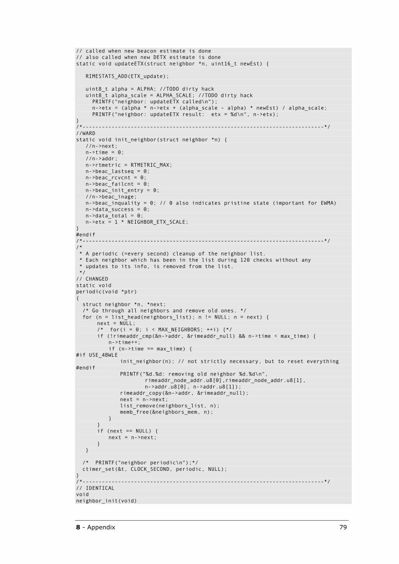
8 - Appendix 79
// called when new beacon estimate is done // also called when new DETX estimate is done static void updateETX(struct neighbor *n, uint16_t newEst) { RIMESTATS_ADD(ETX_update); uint8_t alpha = ALPHA; //TODO dirty hack uint8_t alpha_scale = ALPHA_SCALE; //TODO dirty hack PRINTF("neighbor: updateETX called\n"); n->etx = (alpha * n->etx + (alpha_scale - alpha) * newEst) / alpha_scale; PRINTF("neighbor: updateETX result: etx = %d\n", n->etx); } /*---------------------------------------------------------------------------*/ //WARD static void init_neighbor(struct neighbor *n) { //n->next; n->time = 0; //n->addr; n->rtmetric = RTMETRIC_MAX; n->beac_lastseq = 0; n->beac_rcvcnt = 0; n->beac_failcnt = 0; n->beac_init_entry = 0; //n->beac_inage; n->beac_inquality = 0; // 0 also indicates pristine state (important for EWMA) n->data_success = 0; n->data_total = 0; n->etx = 1 * NEIGHBOR_ETX_SCALE; } #endif /*---------------------------------------------------------------------------*/ /* * A periodic (=every second) cleanup of the neighbor list. * Each neighbor which has been in the list during 120 checks without any * updates to its info, is removed from the list. */ // CHANGED static void periodic(void *ptr) { struct neighbor *n, *next; /* Go through all neighbors and remove old ones. */ for (n = list_head(neighbors_list); n != NULL; n = next) { next = NULL; /* for(i = 0; i < MAX_NEIGHBORS; ++i) {*/ if (!rimeaddr_cmp(&n->addr, &rimeaddr_null) && n->time < max_time) { n->time++; if (n->time == max_time) { #if USE_4BWLE init_neighbor(n); // not strictly necessary, but to reset everything #endif PRINTF("%d.%d: removing old neighbor %d.%d\n", rimeaddr_node_addr.u8[0],rimeaddr_node_addr.u8[1], n->addr.u8[0], n->addr.u8[1]); rimeaddr_copy(&n->addr, &rimeaddr_null); next = n->next; list_remove(neighbors_list, n); memb_free(&neighbors_mem, n); } } if (next == NULL) { next = n->next; } } /* PRINTF("neighbor periodic\n");*/ ctimer_set(&t, CLOCK_SECOND, periodic, NULL); } /*---------------------------------------------------------------------------*/ // IDENTICAL void neighbor_init(void)
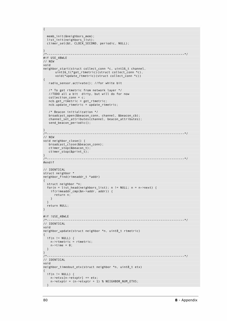
80 8 - Appendix
{ memb_init(&neighbors_mem); list_init(neighbors_list); ctimer_set(&t, CLOCK_SECOND, periodic, NULL); } /*---------------------------------------------------------------------------*/ #if USE_4BWLE // NEW void neighbor_start(struct collect_conn *c, uint16_t channel, uint16_t(*get_rtmetric)(struct collect_conn *c), void(*update_rtmetric)(struct collect_conn *c)) { radio_sensor.activate(); //for white bit /* To get rtmetric from network layer */ //TODO all a bit dirty, but will do for now collection_conn = c; ncb.get_rtmetric = get_rtmetric; ncb.update_rtmetric = update_rtmetric; /* Beacon initialization */ broadcast_open(&beacon_conn, channel, &beacon_cb); channel_set_attributes(channel, beacon_attributes); send_beacon_periodic(); } /*---------------------------------------------------------------------------*/ // NEW void neighbor_close() { broadcast_close(&beacon_conn); ctimer_stop(&beacon_t); ctimer_stop(&print_t); } /*---------------------------------------------------------------------------*/ #endif // IDENTICAL struct neighbor * neighbor_find(rimeaddr_t *addr) { struct neighbor *n; for(n = list_head(neighbors_list); n != NULL; n = n->next) { if(rimeaddr_cmp(&n->addr, addr)) { return n; } } return NULL; } #if !USE_4BWLE /*---------------------------------------------------------------------------*/ // IDENTICAL void neighbor_update(struct neighbor *n, uint8_t rtmetric) { if(n != NULL) { n->rtmetric = rtmetric; n->time = 0; } } /*---------------------------------------------------------------------------*/ // IDENTICAL void neighbor_timedout_etx(struct neighbor *n, uint8_t etx) { if(n != NULL) { n->etxs[n->etxptr] += etx; n->etxptr = (n->etxptr + 1) % NEIGHBOR_NUM_ETXS; }
8 - Appendix 81
} /*---------------------------------------------------------------------------*/ // IDENTICAL void neighbor_update_etx(struct neighbor *n, uint8_t etx) { if(n != NULL) { n->etxs[n->etxptr] = etx; n->etxptr = (n->etxptr + 1) % NEIGHBOR_NUM_ETXS; n->time = 0; } } /*---------------------------------------------------------------------------*/ #endif /* Return the ETX of the specified neighbour (scaled) */ // CHANGED uint16_t neighbor_etx(struct neighbor *n) { #if USE_4BWLE return n->etx; #else int i, etx; etx = 0; for(i = 0; i < NEIGHBOR_NUM_ETXS; ++i) { etx += n->etxs[i]; } return NEIGHBOR_ETX_SCALE * etx / NEIGHBOR_NUM_ETXS; #endif } #if !USE_4BWLE /*---------------------------------------------------------------------------*/ // IDENTICAL void neighbor_add(rimeaddr_t *addr, uint8_t nrtmetric, uint8_t netx) { uint16_t rtmetric; uint16_t etx; struct neighbor *n, *max; int i; PRINTF("neighbor_add: adding %d.%d\n", addr->u8[0], addr->u8[1]); /* Check if the neighbor is already on the list. */ for(n = list_head(neighbors_list); n != NULL; n = n->next) { if(rimeaddr_cmp(&n->addr, &rimeaddr_null) || rimeaddr_cmp(&n->addr, addr)) { PRINTF("neighbor_add: already on list %d.%d\n", addr->u8[0], addr->u8[1]); break; } } /* If the neighbor was not on the list, we try to allocate memory for it. */ if(n == NULL) { PRINTF("neighbor_add: not on list, allocating %d.%d\n", addr->u8[0], addr->u8[1]); n = memb_alloc(&neighbors_mem); if(n != NULL) { list_add(neighbors_list, n); } } /* If we could not allocate memory, we try to recycle an old neighbor */ if (n == NULL) { PRINTF("neighbor_add: not on list, not allocated, recycling %d.%d\n", addr->u8[0], addr->u8[1]); /* Find the first unused entry or the used entry with the highest
82 8 - Appendix
rtmetric and highest etx. */ rtmetric = 0; etx = 0; max = NULL; for (n = list_head(neighbors_list); n != NULL; n = n->next) { if (!rimeaddr_cmp(&n->addr, &rimeaddr_null)) { if (n->rtmetric > rtmetric) { rtmetric = n->rtmetric; etx = neighbor_etx(n); max = n; } else if (n->rtmetric == rtmetric) { if (neighbor_etx(n) > etx) { rtmetric = n->rtmetric; etx = neighbor_etx(n); max = n; } } } } n = max; } /* PRINTF("%d: adding neighbor %d with rtmetric %d, signal %d at %d\n", node_id, neighbors[n].nodeid, rtmetric, signal, n);*/ if(n != NULL) { n->time = 0; rimeaddr_copy(&n->addr, addr); n->rtmetric = nrtmetric; for(i = 0; i < NEIGHBOR_NUM_ETXS; ++i) { n->etxs[i] = netx; } n->etxptr = 0; } } #endif #if USE_4BWLE /*---------------------------------------------------------------------------*/ // NEW /* Return the neighbor with the worst etx value, provided that it is greater * than the given threshold */ static struct neighbor * find_worst_neighbor(uint16_t etx_threshold) { uint16_t etx; struct neighbor *n, *max; PRINTF("neighbor: finding worst neighbor\n"); etx = 0; max = NULL; for (n = list_head(neighbors_list); n != NULL; n = n->next) { if (!rimeaddr_cmp(&n->addr, &rimeaddr_null)) { if (neighbor_etx(n) > etx) { etx = neighbor_etx(n); max = n; } } } if (etx > etx_threshold) { return max; } else { return NULL; } } /*---------------------------------------------------------------------------*/ /* The link will be recommended for insertion if it is better* than some * link in the routing table that is not our parent. */
8 - Appendix 83
// NEW static uint8_t shouldInsert(uint16_t nrtmetric) { struct neighbor *n, *parent; parent = neighbor_best(); /* we assume current parent is current best one */ for (n = list_head(neighbors_list); n != NULL; n = n->next) { if (!rimeaddr_cmp(&n->addr, &rimeaddr_null) && !rimeaddr_cmp(&n->addr, &parent->addr)) { // don't evict parent if (nrtmetric < n->rtmetric) { return 1; //we found a better one, so recommend insertion } } } return 0; } /*---------------------------------------------------------------------------*/ // NEW static struct neighbor * find_random_neighbor() { PRINTF("neighbor: finding random neighbor\n"); int cnt; struct neighbor *n; n = NULL; cnt = neighbor_num(); if (cnt != 0) { n = neighbor_get(random_rand() % cnt); } return n; } /*---------------------------------------------------------------------------*/ // NEW static struct neighbor * try_adding_neighbor(rimeaddr_t *addr, uint16_t nrtmetric) { struct neighbor *n; PRINTF("neighbor_add: adding %d.%d\n", addr->u8[0], addr->u8[1]); /* Check if the neighbor is already on the list. */ n = neighbor_find(addr); /* If the neighbor was not on the list, we try to allocate memory for it. */ if (n == NULL) { PRINTF("neighbor_add: not on list, allocating %d.%d\n", addr->u8[0], addr->u8[1]); n = memb_alloc(&neighbors_mem); if (n != NULL) { list_add(neighbors_list, n); } } /* If we could not allocate memory, we try to recycle an old neighbor */ if (n == NULL) { PRINTF("neighbor_add: not on list, not allocated, recycling %d.%d\n", addr->u8[0], addr->u8[1]); /* Find the first unused entry or the used entry with the highest * etx that is above a certain theshold */ n = find_worst_neighbor(EVICT_ETX_THRESHOLD); } /* If we still could not allocate memory: * If the white bit is set, lets ask the router if the path through this link * is better than at least one known path - if so lets insert this link into * the table. */ if (n == NULL) { PRINTF("White bit selection mechanism\n"); if (is_high_channel_quality() == 1) {
84 8 - Appendix
if (shouldInsert(nrtmetric) == 1) { n = find_random_neighbor(); PRINTF("Neighbor %d.%d will be evicted.\n", n->addr.u8[0], n->addr.u8[1]); } else { PRINTF("The upper layer advised not to insert the neighbor\n"); } } else { PRINTF("Channel quality not high enough to consider insertion\n"); } } /* If we found an entry, update it */ if (n != NULL) { n->time = 0; rimeaddr_copy(&n->addr, addr); init_neighbor(n); n->rtmetric = nrtmetric; } return n; } #else /*---------------------------------------------------------------------------*/ // IDENTICAL void neighbor_remove(rimeaddr_t *addr) { struct neighbor *n; for(n = list_head(neighbors_list); n != NULL; n = n->next) { if(rimeaddr_cmp(&n->addr, addr)) { PRINTF("%d: removing %d\n", rimeaddr_node_addr.u8[0], addr->u8[0]); rimeaddr_copy(&n->addr, &rimeaddr_null); n->rtmetric = RTMETRIC_MAX; list_remove(neighbors_list, n); memb_free(&neighbors_mem, n); return; } } } #endif /*---------------------------------------------------------------------------*/ /* * Return the neighbor with the lowest combined rtmetric & history-averaged * etx value */ // IDENTICAL struct neighbor * neighbor_best(void) { int found; /* int lowest, best;*/ struct neighbor *n, *best; uint16_t rtmetric; rtmetric = RTMETRIC_MAX; best = NULL; found = 0; /* PRINTF("%d: ", node_id);*/ /* Find the lowest rtmetric. */ for(n = list_head(neighbors_list); n != NULL; n = n->next) { if(!rimeaddr_cmp(&n->addr, &rimeaddr_null) && rtmetric > n->rtmetric + neighbor_etx(n)) { rtmetric = n->rtmetric + neighbor_etx(n); best = n; } } return best;
8 - Appendix 85
} /*---------------------------------------------------------------------------*/ /* * Set the time to keep neighbors in the neighbor table. * Time = amount of periods of periodic table cleanup * (currently set to: 120 x 1 sec = 120 seconds) */ // IDENTICAL void neighbor_set_lifetime(int seconds) { max_time = seconds; } /*---------------------------------------------------------------------------*/ /* * Return the number of neighbors in the table */ // IDENTICAL int neighbor_num(void) { PRINTF("neighbor_num %d\n", list_length(neighbors_list)); return list_length(neighbors_list); } /*---------------------------------------------------------------------------*/ /* * Return the num-th neighbor in the table */ // IDENTICAL struct neighbor * neighbor_get(int num) { int i; struct neighbor *n; PRINTF("neighbor_get %d\n", num); i = 0; for(n = list_head(neighbors_list); n != NULL; n = n->next) { if(i == num) { PRINTF("neighbor_get found %d.%d\n", n->addr.u8[0], n->addr.u8[1]); return n; } i++; } return NULL; } /*---------------------------------------------------------------------------*/
86 8 - Appendix
8.5 AppendixE–Reportedbugs
The following is a list of bugs that have been discovered and subsequently reported to the Contiki developer mailing list:
• Developer mailing list, December 6, 2008: MIN/MAX bug in core/net/rime/polite.c and ipolite.c. The bug was fixed upon a second report to the mailing list.
• Developer mailing list, March 15, 2009: the runicast-stunicast bug where the number of transmissions is incorrectly handled (see § 3.4).
• Developer mailing list, April 7, 2009: suggestion for some minor coding enhancements (not bugs) to core/net/rime/collect.c. These were incorporated in the CVS in version 1.24 of collect.c.
• Developer mailing list, April 27, 2009: reported a bug in the msp430 compiler concerning integral promotion.
• Developer mailing list, April 29, 2009: reported and suggested a fix for a forwarding flag bug in core/net/rime/collect.c. The bug was confirmed, but was countered the same day by the implementation of a packet queue for collect.c.