Crosshole radiowave surveys (RIM) in borehole …Crosshole mise á la masse results agree well with FARA results. Crosshole radiowave imaging is applicable in Olkiluoto for detecting

P O S I V A O Y

Olk i luo to

F I -27160 EURAJOKI , F INLAND

Te l +358-2-8372 31

Fax +358-2-8372 3709

Arto Korp i sa lo , Ta rmo Jok inen

N iko laev Popov , A lexander Shuva l -Sergeev ,

T imur Zh ienbaev

Eero He ikk inen , Jo rma Nummela

November 2008

Work ing Repor t 2008 -79

Review of Crosshole Radiowave Imaging (FARA)in Drillhole Sections OL-KR4 – OL-KR10 and

OL-KR10 – OL-KR2 in Olkiluoto, 2005

November 2008

Working Reports contain information on work in progress

or pending completion.

The conclusions and viewpoints presented in the report

are those of author(s) and do not necessarily

coincide with those of Posiva.

Arto Korp isa lo , Tarmo Jok inen

Geo log ica l Su rvey o f F in l and

Niko laev Popov , A lexander Shuva l -Sergeev ,

T imur Zh ienbaev

FGUNPP (Geo logorazvedka )

Eero He ikk inen , Jorma Nummela

Pöyry Env i ronment Oy

Work ing Report 2008 -79

Review of Crosshole Radiowave Imaging (FARA)in Drillhole Sections OL-KR4 – OL-KR10 and

OL-KR10 – OL-KR2 in Olkiluoto, 2005

Review of Crosshole Radiowave Imaging (FARA) in Drillhole Sections OL-KR4 – OL-KR10 and OL-KR10 – OL-KR2 in Olkiluoto, 2005

ABSTRACT Posiva Oy carries out research and development of spent nuclear fuel disposal in Finland. The repository will be constructed deep in the crystalline bedrock in Olkiluoto island in Eurajoki. Construction of underground characterization facility ONKALO started 2004.

Posiva Oy and ANDRA, France have co-operated in reviewing the methods for granitic i.e. crystalline bedrock characterization methods. One of the considered themes was electromagnetic crosshole survey. This report describes field work, interpretation and review of crosshole radiowave imaging (RIM) using FARA-MCH tool in 2005 between two drillhole panels at 200-600 m depth level. Drillholes are separated 150-400 m. The works were jointly carried out by Geological Survey of Finland and FGUNPP “Geologorazvedka” (Russia).

FARA tool feasibility in characterization of deformation zones and lithological domains was tested. Geological–geophysical characterization of Olkiluoto site has run since 1989, and more than 40 drillholes have been prepared. Background information is abundant for comparisons with, e.g., geophysical logging, electrical and electromagnetic sounding, and seismic imaging and reflection sounding.

Olkiluoto migmatitic bedrock has undergone a polyphasic ductile–brittle deformation. Resistivity in bedrock varies strongly in range of tens to tens of thousands of Ohm.meters.

FARA–MCH electrical dipole receiver and transmitter probes are connected and synchronized with wireline. The cable interference is suppressed with filters. The method operates in inductive field domain and the field measurables are amplitude and phase difference. at four separate frequencies 312.5, 625, 1250 and 2500 kHz. For each transmitter station at 20–70 m spacing a continuous scan of 200–450 m was measured at 0.5 m interval. Field work was finalised within a week successfully despite of strong noise encountered. Phase information was not used due to noise level. Preliminary processing and quality control was finalised on site.

In processing the amplitude signal was cleaned of outliers and normalised by distance and geometry to obtain attenuation (dB/m), and a tomographic reconstruction was carried out to obtain resistivity in 5 x 5 m or 10 x 10 m cell size, using drillhole resistivity as constraint. Detected low and high resistivity zones, and their apparent shapes and orientations, agree well between the two sections and are in fair agreement with geological and other geophysical results. Material properties are different than in seismic tomography from same location, though reflections describe partly the boundaries of domains differing in electrical properties. Same but more detailed information is obtained as in electric and electromagnetic results from ground surface. Crosshole mise á la masse results agree well with FARA results.

Crosshole radiowave imaging is applicable in Olkiluoto for detecting of conductive and resistive domains, rather than unique fractures or zones. For objects of adequate contrast to be observed, minimum thickness is 20–30 m, and length dimension larger. Drillhole

deviation and recorded depth correctness are critical for successful interpretation. The attenuation is associated with conductivity variation (fracturing and sulphide content) whereas the phase difference would supplement with dielectric permittivity (water content, lithology). Magnetic susceptibility is not used in interpretation, but its variation may affect the results.

The field work should be carried out with denser 5–10 m transmitter interval for higher resolution. Receiver spacing 0.5 m is reasonable. Frequencies 312.5 and 625 kHz apply to distances of 300…400 m, and in some cases with 1250 kHz to 150…200 m., Depth section should be adequately long and drillholes close to a common plane. The inversion method and parameters should be carefully selected, and the interpretation developed to apply 2D/3D numerical modeling.

Keywords: Spent nuclear fuel, geological disposal, Olkiluoto, migmatitic gneiss,

ductile deformation, brittle deformation, radiowave imaging, FARA, drillhole

geophysics

Olkiluodon reikien OL-KR4 – OL-KR10 ja OL-KR10 – OL-KR2 välisen radiovarjostusmittauksen (FARA, 2005) tulosten arviointi

TIIVISTELMÄ

Posiva Oy huolehtii käytetyn ydinpolttoaineen loppusijoitukseen liittyvistä tutkimus- ja kehitystehtävistä Suomessa. Loppusijoitustilat rakennetaan syvälle kiteiseen perus-kallioon Olkiluodon saaressa Eurajoella. Maanalaisia ONKALO tutkimustiloja on louhittu 2004 lähtien.

Posiva Oy ja ANDRA (Ranska) ovat yhteistyössä selvittäneet graniittisen (kiteisen) kiven tutkimusmenetelmiä. Yksi käsiteltävistä teemoista on ollut sähkömagneettinen reikien välinen mittaus. Tämä raportti käsittelee 2005 kahdessa reikäleikkauksessa 200-600 m syvyydellä tehtyä FARA -radiovarjostusta, sen tulkintaa ja tulosvertailua. Reikien etäisyys on 150-400 m. Mittauksen tekivät GTK ja venäläinen FGUNPP Geologoradzvedka tarkoituksena testata menetelmän kykyä kuvailla deformaatio-vyöhykkeitä ja kivilajiominaisuuksia. Olkiluodon kallioperää on tutkittu geologisissa ja geofysikaalisissa tutkimuksissa vuodesta 1989, ja alueella on tehty yli 40 syvää kairanreikää, joista on saatavilla tietoa geofysiikan reikämittauksista, sähköisistä ja sähkömagneettista luotauksista, sekä seismisistä tomografia- ja heijastustuloksista vertailua varten. Olkiluodon migmatiittinen kallioperä on käynyt läpi monivaiheisen plastisen ja hauraan deformaation. Kallion sähköinen ominaisvastus vaihtelee voimakkaasti joistakin kymmenistä kymmeniin tuhansiin ohmimetreihin.

FARA-MCH sähköinen dipolilähetin ja -vastaanotin on kytketty toisiinsa ja synkronoitu kaapelin avulla. Signaalin suora kaapeliyhteys vaimennetaan suotimin. Menetelmä toimii sähkömagneettisen kentän induktiivisessa alueessa, ja mittausparametrit ovat kentän amplitudi ja vaihe-ero neljällä eri taajuudella 312.5, 625, 1250 ja 2500 kHz. Jokaiselle 20–70 m välein sijainneelle lähetinasemalle mitattiin jatkuva, 200–450 m pitkä profiili 0.5 m välein. Kenttätyö valmistui viikossa hyvin tuloksin vaikka kohinataso oli voimakas. Vaihetietoa ei voitu käyttää häiriöiden vuoksi. Alustava tuloskäsittely ja laadunvarmennus tehtiin tutkimusalueella.

Prosessoinnissa amplitudisignaalista poistettiin häiriöt ja se normalisoitiin etäisyyden ja geometrian suhteen vaimennukseksi (dB/m). Tomografisena rekonstruktiona tuotettiin ominaisvastus solukokoon 5 x 5 tai 10 x 10 m, käyttäen reikien loggaustuloksia rajoittimena. Todetut matalan ja korkean ominaisvastuksen tilavuudet sopivat geologisiin ja muihin geofysikaalisiin reikätuloksiin. Materiaalitiedot liittyvät eri para-metreihin kuin seismisissä tuloksissa, joissa on ainakin paikoin esillä sähköisesti poikkeavien tilavuuksien rajapintoja. Tieto on vastaavaa mutta tarkempaa kuin maanpinnalta tehdyissä sähköisissä ja sähkömagneettisissä luotauksissa. Lataus-potentiaalimittaukset sopivat FARAn kanssa yhteen.

FARA soveltuu Olkiluodossa reikien väliseen laajojen johtavien ja eristävien tilavuuksien paikantamiseen, kun kontrastit ovat riittävät. Näitä ovat kivilajiyksiköt ja deformaatiovyöhykkeet ennemmin kuin yksittäiset rakoiluvyöhykkeet. Kohteiden paksuusluokka on noin 20–30 m, ja pituussuuntainen jatkuvuus tätä suurempi. Reikien taipumatietojen ja laitteiden syvyystiedon oikeellisuus on kriittinen tulkinnan onnistumiseksi. Vaimennus liittyy johtavuusvaihteluun (rikkonaisuus, sulfidipitoisuus), jota vaihe-ero täydentäisi tiedolla sähköisestä dielektrisyydestä (vesipitoisuus, kivilajit). Magneettista suskeptibiliteettiä ei ole käytetty tulkinnassa, mutta se vaikuttanee tuloksiin.

Kenttätyö tulisi suorittaa melko tiheällä, 5–10 m lähetinvälillä kairanrei’issä erotus-kyvyn parantamiseksi. Vastaanotinasemien tiheys 0.5 m on riittävä. Menetelmä on Olkiluodossa toimiva matalimmilla 312.5 ja 625 kHz taajuuksilla 300…400 m reikä-etäisyydelle, ja joissakin tapauksissa 1250 kHz taajuudella 150…200 m reikä-etäisyydelle. Reikien keskinäisen asennon tulisi olla lähellä tasomaista, ja tutkittavan leikkauksen riittävän syvä etäisyyteen nähden. Inversiomenetelmä ja sen asetukset pitäisi valita huolella, ja tulevaisuudessa kehittää numeerista 2D- tai 3D- mallinnus-menetelmää.

Avainsanat: Käytetty ydinpolttoaine, geologinen loppusijoitus, Olkiluoto, magma-tiittinen gneissi, plastinen deformaatio, hauras deformaatio, radioaaltokuvantaminen, FARA, reikägeofysiikka.

1

TABLE OF CONTENTS ABSTRACT TIIVISTELMÄ PREFACE

1 INTRODUCTION................................................................................................... 5 2 OPERATING PRINCIPLES OF RADIO IMAGING METHOD ................................ 7 3 FARA–MCH FIELD INSTRUMENTATION .......................................................... 15 4 FIELD WORK AND QUALITY CONTROL ........................................................... 17 5 PROCESSING AND INTERPRETATION ............................................................ 27 6 RESULTS ........................................................................................................... 35 6.1 Drillhole panel OL-KR4–OL-KR10 ................................................................. 35 6.2 Drillhole panel OL-KR10 – OL-KR2 ............................................................... 40 7 COMPARISON WITH DRILLHOLE AND OTHER GEOPHYSICAL DATA .......... 45 7.1 Reviewing the FARA results .......................................................................... 45 7.1.1 Checking the data against logging ................................................................ 45 7.1.2 Internal consistency of FARA tomograms...................................................... 52 7.2 Comparison of FARA results to other data .................................................... 58 7.2.1 Comparisons to drillhole results .................................................................... 58 7.2.2 Comparisons to electromagnetic sounding results ........................................ 69 7.2.3 Comparisons to electrical pole–pole sounding results ................................... 71 7.2.4 Comparison to Mise á la masse results ......................................................... 73 7.2.5 Comparison to seismic crosshole tomography and reflector model ............... 74 8 DISCUSSION ...................................................................................................... 83 REFERENCES ........................................................................................................... 87

2

3

PREFACE

This work has been carried out at Geological Survey of Finland (GTK) on contract for Posiva Oy “Radiowave shadowing (FARA) tomography between Olkiluoto drillholes KR4–KR10 and KR10–KR2 in 2005”, Posiva's order number 9814/05/TUAH. Supervising of the field work was done by Turo Ahokas (Posiva) and Eero Heikkinen (Pöyry Environment Oy).

Posiva, Finland and Andra, France (Dr. Yannick Leutsch) co-operated in this project for review and information exchange. Measurements and processing were co-operated with FGUNPP (Geologorazvedka, St. Petersburg). Field work interpretation and reporting were done by Arto Korpisalo and Tarmo Jokinen (GTK) and Nikolai Popov, Alexander Shuval-Sergeev and Timur Zhienbaev (FGUNPP).

Review of other geophysical information was carried out by Pöyry Environment Oy (Eero Heikkinen). Comparison images were compiled by Jorma Nummela. Kind comments from Pauli Saksa and Pirjo Hellä (Pöyry Environment Oy) and Ilmo Kukkonen (GTK) were considered in this report.

Field survey group. From the left: Tarmo Jokinen, Arto Korpisalo, Konstantin Avdeev,

Nikolaev Popov, Timur Zhienbaev and Alexander Shuval-Sergeev.

4

5

1 INTRODUCTION

Posiva Oy carries out the spent nuclear fuel related research and development in Finland. Work is focused in Olkiluoto, Eurajoki. Underground characterization premises ONKALO have been constructed since 2004. Andra, France and Posiva have co-operated in feasibility assessment of granitic area investigation methods, among them electromagnetic crosshole imaging.

Crosshole radiowave imaging (RIM) was tested 2005 in two drillhole pairs. Method background is in coal mapping and exploration, where conductive bodies and their distance and location azimuth can be detected even when these are not intersected. Resistive coal seams function as wave guides, and termination of seam can be observed to distances of 600 m from transmitter. Previous works in Finland have not been reported. Method was estimated feasible in Olkiluoto because of strong conductivity variation. Conductivity changes according to sulphide content of the rock mass, due to groundwater salinity variation, and due to fracturing. Frequency range of RIM, from hundreds to thousands of kilohertz, is higher than in common electromagnetic soundings. This enables higher spatial resolution, which is further enhanced by drillhole geometry directly applied in investigation volume. Still frequency is lower than in ground penetrating radar, producing greater investigation range, even in conductive or in magnetic environment (Redko et al. 2000, Stevens et al. 1998). Electromagnetic field is diffuse rather than a propagating wave front, making interpretation more demanding.

Comparison to abundantly available background information was included into this work. Data sets contained seismic reflection and tomographic crosshole results, electromagnetic and electrical ground level models, electrical crosshole mise á la masse data, and geological and geophysical drillhole logging information from measured drillholes. External check was possible using data from drillhole OL-KR14, located in the vertical plane defined by OL-KR4–OL-KR10–OL-KR2, but was not included in FARA survey or processing.

Project was set between Posiva Oy and Geological Survey of Finland (GTK). The clients Andra and Posiva defined the tasks and organised the site and background information for use. Pöyry Environment Oy consulted in design and review of field work. GTK co–operated measurements using FARA-MCH drillhole tool and processing with its Russian developer and manufacturer, FGUNPP “Geologorazvedka” who provided advisory expertise in field work and processing. GTK organised the tools, interpreted the data and compiled the report. Field work took place in drillholes OL-KR4, OL-KR10 and OL-KR2 in October–November 2005. Results were processed and delivered by December 2005. Actual image data was receiver later in 2006, and the review was revised to accommodate data quality estimate. Numerical EM modelling was not included into the task.

Field work and processing is presented in Chapters 2–6, as written by Nikolaev Popov, Alexander Shuval-Sergeev and Timur Zhienbaev of FGUNPP and Arto Korpisalo and Tarmo Jokinen of GTK. Results of the review are presented in Chapter 7, written by Eero Heikkinen (Pöyry Environment Oy), who also edited the report text. Review includes presentation of comparison data and performance review of seismic and FARA crosshole methods with comments concerning applicability of the method.

6

7

2 OPERATING PRINCIPLES OF RADIO IMAGING METHOD Radiowave shadowing method (RIM) was developed in the early 1980’s to detect hazards or obstructions in coal panels prior to long-wall mining. Method was successful because the coal seam, having electrical resistivity substantially greater than in the surrounding geology, act as EM wave-guide. The wave-guide allows reasonably high frequencies to be transmitted and received at distances of almost 600 meters. Method can be applied in drillhole to detect conductive bodies and their location azimuth and orientation, even when these are not intersected. Recently the technique has been applied in crosshole imaging mode, and successfully operated also in crystalline bedrock environment in exploration (Redko et al. 2000, Stevens et al., 1998).

Crosshole EM survey has several clear benefits over the ground level electromagnetic sounding methods. Applying a drillhole source brings the survey closer to the target, and will allow usage of higher frequencies and thus enables a higher resolution. Another benefit is possibility to view the target from different angles and directions, not only in vertical direction and from above. Placing the source in drillhole also will enable getting rid of boundary effects related to ground surface and strong attenuation emerging from soil deposits. Drawback is availability and location of drillholes, limited power of transmission of drillhole probe, and a relatively complex behavior of 3D source field within subsurface target, which is difficult to resolve numerically without significant approximations.

The physical behaviour of electromagnetic field in rock is governed mathematically by Maxwell equations. Behaviour varies with distance R from the source. Maxwell's equations describe constitutive relationship and quantify material properties. EM theory on field properties in conductive media and the consequencies for FARA application has been thorougly treated in GTK's Q-report (Korpisalo 2005). This report will refer the key issues.

The time-dependent electromagnetic field interaction in medium can be written according to Maxwell’s equations in differential form.

According to Faraday’s induction law (1) and Ampère–Maxwell’s law (2) the curl of

electric field strength E is comparable to time derivative of magnetic flow density B ,

8

and curl of magnetic flow density B comparable to sum of current density J and time

derivative of electric displacement vector D (electrical flow density).

According to Gauss’s law for electrical and magnetic scalar fields (3 and 4), the

divergence of electric displacement vector D (3) equals to electric charge q, and

divergence of magnetic field density B is zero.

Governing physical properties in electromagnetic interaction in bedrock are the

electrical conductivity ~ , dielectric permittivity ~ , and magnetic permeability ~ .

These tensor quantities define how the medium will interact with electrical field

strength E and magnetic field strength H to procude the flow densities. The material

properties are linking the field and flow properties as

and

First approximation in FARA surveys is to consider these properties linear, i.e., scalars

parallel to source field and independent of source field strength.

Time–alternating E and H fields are intercoupled, and the components are induced

from each another, e.g., magnetic field creates electric fields, vice versa. The fields may

be according to relative rate of loss encountered in medium either in the inductive

(diffuse) or propagating (radio) wave fields.

Eliminating magnetic field from Maxwell’s equations using Faraday’s law (1) and

Ampère–Maxwell’s law (2), is obtained Helmholtz equation for electric field (8):

According to (8), electrical field vectors depend on magnetic permeability and electrical

conductivity, and magnetic permeability and dielectrical permittivity. Eliminating the

electric field, equation of same form would be obtained for magnetic field.

Wave equation form, depending on angular velocity, instantaneous field vector sE can

be written as

9

Expressing complex permittivity εc as in (10) is get

where the loss tangent

is a ratio of conductivity and displacement currents.

One can define square of propagation constant or wavenumber γ (11) as

Propagation constant allows to define the electrical field into (12)

where α (real part of propagation constant) is attenuation rate and imaginary part β is

the phase constant. These properties define how the field is attenuated and phase shifted

according to time and distance. For propagating wave field, in ideal lossless medium

would be α = 0.

Writing solution for propagation constant (13)

Three different zones are generally defined in the terms of wavelength or inverse loss

tangent Q, which are the near field zone (Q<<1, R << ), the intermediate zone (Q

R ) and the far field (the radiative) zone (Q>>1, R>>).

For low frequency and high conductivity domain the inductive (diffusive) equation is

applying the middle term ωμε, attenuation is dominated by conductivity, and effect of

dielectric permittivity is negligible. In high frequency and low conductivity domain the

wave equation is effective (real part, –ω2με), and attenuation will depend dominantly on

dielectric permittivity.

For propagating wave field the electromagnetic interaction is described by wavefront

velocity, angular velocity, wave length, phase, polarization, and attenuation.

In transition domain between diffusive and wave field behaviour, both Re and Im parts

of the equation need to be considered, and attenuation and phase are dependent both on

dielectric permittivity (displacement currents) and conductivity. A transition frequency

10

ftr where displacement currents and conductivity are equal in relative magnitude, is

expressed as (14):

For typical average values of relative dielectric permittivity εr: 6–8 and conductivity ζ:

0.001–0.0001 S/m in Olkiluoto bedrock, the transition frequency gets values of 200–

3000 kHz, i.e., exactly the range of FARA survey in the area. It is also useful to

remember that the dielectric permittivity decreases and conductivity increases according

to increasing frequency.

On neglecting the magnetic permeability µ, in limited domains in Olkiluoto the

susceptibility κ may approach 1, which would require encountering also magnetic

properties.

11

Figure 1. Schematic drawing of FARA transmitter and receiver dipoles and the

effective field components. Tangential electric field Eθ perpendicular to path is

normalised with distance l and with the receiver and transmitter angles to field vector.

The magnetic axial BΦ and electriacl radial ER are not encountered.The paths passing

through cells C are minimised computing line integral of attenuation over cells.

The electromagnetic source in FARA probe is electrical dipole antenna which is aligned

parallel to drillhole axis (Figure 1). The generated 3D dipole field is separated into axial

magnetic B and polarized radial and tangential electrical E vector components (Figure

1). Maximal coupling for the E field is in E-polarization, when the field component is

12

parallel to the conductive target to be surveyed. This will depend both on orientation of

the target and orientation of the field components.

EM field properties are depending strongly on distance from the source, and on the

physical parameters. Inverse of the loss tangent (10), or ratio of real and imaginary part

of wavenumber γ (11), describes the wave field behaviour

When Q >> 1 the dielectric properties are dominant, EM field propagates as wavefront

through medium and all frequency components travel roughly at same velocity (non–

dispersively), encounter the same attenuation α, and the waveform remains non altered

through passage. Velocity v and attenuation α are presented for propagating wave field

as

Attenuation α is depending on dielectric permittivity and electrical conductivity ζ.

When Q<< 1 the velocity v is independent of dielectric permittivity , but is controlled

by conductivity ζ, and the EM field is diffuse. The energy distribution is dispersive, i.e.

attenuation α will depend on conductivity and frequency (f, or angular velocity ).

In diffuse domain the attenuation can be also described in terms of skin depth δ (19), a

distance where the field at each frequency has attenuated to e–1

fraction of initial field

strength (for diffuse plane wave).

The attenuation will depend on distance from the source. Wavenumber γ times distance

r defines the attenuation behaviour. When │γr│< 1 (distances shorter than wavelength),

field attenuation resembles static dipole behaviour r–3

, and when │γr│= 1, attenuation is

governed by distance, wavenumber, exponential decay, and geometric decay. In far

field, when │γr│>> 1 (distances much greater than wavelength), attenuation is

depending inversely on distance, r-1

. This is the case on which FARA crosshole

tomographic interpretation is based on.

13

For low <300 kHz frequencies and short < 50 m distances, and for resistivities <1000

Ohm.m, the FARA operates in near field domain. When frequencies increase >1000

kHz, distances extent >100 m and resistivities approach 10000 Ohm.m, the case is, or is

approaching, the far field. Mostly the behavior takes place in intermediate field,

meaning the near field effects will affect occasionally.

Considering parameter loss tangent or its inverse Q, at the frequency range of 300–2500

kHz the electromagnetic signal behaviour is in intermediate (Q 1) transition domain

between propagating radiowave (high Q >> 1) and diffuse EM field (low Q < 1). In the

transitional domain both dielectric permittivity and electrical conductivity will affect to

attenuation.

True propagating EM wave field is used in radar, with frequencies >10 MHz and wave

lengths < 20 m, but also with limited range. Field properties would be characterized by

travel time, amplitude and reflection. In purely inductive EM field at frequencies < 100

kHz and for > 300 m wave lengths, the interaction would be characterized by frequency,

skin depth, attenuation, and phase difference.

As presented in (Korpisalo 2005), the wave velocity at the FARA frequency range and

dominant relative dielectric permittivity range, εr: 6,5–8, does not depend on

conductivity but on dielectric permittivity, when conductivity is less than ζ < 10-4

S/m.

When conductivity is higher than ζ > 10-2

S/m, velocity is not affected by dielectric

permittivity. At conductivity range ζ: 10-4

–10-2

S/m the velocity v depends on

conductivity ζ and changes from 100…120 m/µs to 50…70 m/µs. Velocity v would be

rather good tool to analyse conductivity distribution, but it is not an interpretation

parameter, as the arrival time is not recorded, despite of synchronization.

Considering the understanding of near and far fields, and high and low Q domains, it is

useful to take the wavelength into account. In the same range of dielectric permittivity

εr and frequencies f, the wavelength is depending on dielectric permittivity εr,

conductivity ζ, and frequency f. At conductivity ζ < 10-4

S/m the wavelength

depends on dielectric permittivity εr and frequency f, ranging at relevant dielectric

permittivity range, εr: 6,5–8, at 35–320 m. At conductivity ζ > 10-2

S/m the

wavelength is little depending on dielectric permittivity εr, and according to frequency

it is varying at 20–60 m. Nevertheless in diffuse EM field domain, and in transition

between near and far field, for resolution the wavelength cannot be directly applied as

a resolution criteria. Cell sizes in inversion are fractions of the wavelength as in true

traveltime tomography there should not be more than 2–4 cells on each cycle.

Attenuation is strongly depending on conductivity at the FARA frequencies. At the

dielectric permittivity range of Olkiluoto rocks, εr: 6,5–8, the dielectric permittivity has

a minor influence to attenuation α. Increasing frequency f increases the attenuation α the

more the conductivity ζ increases. At conductivity range ζ: 10-4

–10-2

S/m, the

attenuation α ranges from 0,05…0,06 dB/m to 1…2,5 dB/m. As the amplitude is the

directly measurable parameter, it can be used to estimate conductivity ζ, bearing in

mind the following limitations:

- attenuation α is formulated for tangential, E–polarised electrical field component

of the dipole antenna having 1/r attenuation in intermediate - far field

14

- formulation holds for isotropic, locally homogeneous medium, any deviations

from this condition will affect also the results.

- the near field effects cause also other polarizations, radial E–field component

with different attenuation α, and static field behavious attenuation related to 1/r3

present; closer than 50–100 m distances need to be considered for these effects.

- off plane conductive targets will also affect strongly to the diffuse field results,

i.e. the “ray” is actually not a ray, but the shortest distance and the field angle

used in normalisation!

- regarding the above stated, numerical inverse modeling would resolve in more

detail the case, where tomogram would be used as a starting model (seed).

It is necessary to understand these fundamantal terms in interpreting FARA results. For

this reason also the full solution of Maxwell’s equations for electrical dipole field would

be useful. In practical tomographic reconstruction an approximation is adequate. There

is yet not available any software, which can take into account the whole wave equation

solution.

In FARA field solution, only amplitude attenuation and phase difference are considered.

Signal velocity, wave length, or phase behaviour is not taken into account. The

amplitude and phase difference data can be interpreted to indicate locations, where the

wave is attenuated or shadowed due to conductive structures. Using three components

would resolve some of geometrical ambiguities. Applying similar crosshole

measurement geometry in time domain would lead to some benefits over the continuous

signal, single frequency amplitude decay approach. One of these is the measurement

during signal off- time.

Important approximation is to consider the survey volume a full space, without taking

the boundary conditions at ground surface into account. Normally in tomography a far

field condition is assumed where source and transmitter are separated by several

wavelengths, which is not completely true in FARA survey, but the approximation

makes interpretation much easier. A further approximation has been made to handle

only electrical conductivity. However the interaction will include also influence of

magnetic and dielectric properties of the rock. In the intermediate domain the

Maxwell’s equations should be preferably completely written open to account the

electrical conductivity, attenuation, magnetic susceptibility, dielectric permittivity and

phase difference.

Spatial variations in physical properties in the survey volume are observed as variation

in received amplitude. In the linear approximation of electrical field, the amplitude is

normalised for distance and dipole field geometry, as deviation from normal of the field

both in transmitter and receiver (maximum field intensity is measured at dipole axis).

The attenuation rate (amplitude loss normalised over distance) is computed to describe

conductivity variation. Multiple pairs of transmitter stations and dense scans over large

angle window can be used to reconstruct a tomographic image on conductivity in a

similar way as for DC Electrical Resistivity Imaging (ERT), which can give geometric

idea on conductivity variation. Inversion will compute resistivity values for cells, which

have attenuation per unit length values (rays) assigned passing through (see Chapter 4

below).

15

3 FARA–MCH FIELD INSTRUMENTATION

The FARA tool is operating simultaneously at maximum four frequencies, 312.5, 625,

1250 and 2500 kHz. Measuring together all frequencies reduces survey time essentially.

Transmitter power is divided between the frequencies, thus highest power is obtained

using a single frequency.

A 35 m long, 36 mm in diameter radio antenna (electrical dipole antenna aligned with

drillhole axis) is used in transmitting signal into the bedrock. Amplitude and phase of E-

polarized electric field component along receiver drillhole axis are measured.

The signal timing and phase are synchronized between transmitter and receiver units via

wireline. This allows the receiver phase relative to transmitter to be measured.

Reference signal improves considerably the tool sensitivity and noise immunity. Special

damping filters are used avoid interference and suppressing the antenna effect off in the

wireline.

Measurements are controlled and information recorded with laptop computer and 32-bit

MS Windows software. The automated measurement process requires operator’s

minimal intervention. The operator can monitor the data quality at all the frequencies in

real time, and view previous results. This allows adjustments in survey depth range and

sampling density, and will enable decision on re-measurement.

System is consisted of control unit, recording units, set of transmitter and receiver

downhole antennae, winch for transmitter and receiver, depth encoder and connecting

cables (Figure 2). Two down–hole cable types of 600 m in length were used, the other

with polyurethane insulation (FGUNPP) and the other steel armoured (GTK). GTK

cable was equipped with FARA adapter to connect the probe.

Technical specifications of the FARA-MCH system are given in the Table 1 below:

Table 1. System information.

Parameter Data

Operating frequencies 312.5, 625, 1250 and 2500 kHz

Measurement voltage range 0.03–1000 µV, +/–10%

Measurement phase difference range 0–360 degrees, +/–5 degrees

Transmitter power 1 W

Cable length (2005) 600 m

Diameter of downhole probe 36 mm

Length of downhole probe 35 m

Max depth of operation 3000 m

16

Figure 2. FARA equipment. The receiver unit (above), the transmitter unit (below), the

antenna (below) and necessary cables, transmitter and receiver tubes, and a small

surface filter are included.

17

4 FIELD WORK AND QUALITY CONTROL

The task of the field work was to test feasibility of the method with respect to known

site properties, and to provide further information on shape and continuity of the

resistive and conductive bodies in the subsurface.

Measurements were carried out in Olkiluoto at two drillhole pairs located roughly on a

same North–South traverse (Easting 1526.000 in Finnish KKJ1 datum). Measurements

were carried out in OL-KR4 and OL-KR10 in the south, and drillholes OL-KR10 and

OL-KR2 in the north.

Diamond drilled holes are water filled, equipped with steel casing to 40 m, and 56 mm

(OL-KR2 and OL-KR4) or 76 mm (OL-KR10) in diameter. Drillholes OL-KR2 and

OL-KR4 are 15–20 degrees tilted from vertical, and their azimuth aligned roughly

towards the North. Drillhole OL-KR10 is almost vertical, tilted 5–12 degrees.

Length of drillholes ranges from 614 m (OL-KR10) to 900 m (OL-KR4) and 1050 m

(OL-KR2). The distances between the drillhole collars were 250 and 300 m and shortest

distances between the drillholes 150–200 m (OL-KR4 to OL-KR10) and 300–400 m

(OL-KR10–OL-KR2). Section ranging from vertical depth 200–600 m was surveyed in

this work.

The highest position of the survey is set approx. to the distance between the drillholes,

to avoid boundary effects of ground surface in interpretation (full space field

approximation). In designing a crosshole profile, the panel depth extent shall be longer

than horizontal distance between the drillholes. Depth of panels was limited by

available cable length (600 m) and depth of OL-KR10.

Before measurements the openness of the drillholes was carefully ensured with dummy

probe. Transmitter is set at a selected depth level in a drillhole. The transmitter stations

were placed at 20 m spacing in OL-KR4, 40 m spacing in OL-KR10 and 70 m spacing

in OL-KR2. Spacing is set to the order of 1/10 of the drillhole distance. Spacing was

first selected 20 m because the conductivity structure was not exactly known. After

preliminary results the spacing was increased to 40 m. The 40 m spacing was applied

also for drillhole pair OL-KR10–OL-KR2. Due to difficulties met in winch operation,

spacing was increased to 70 m for scans from OL-KR2 to OL-KR10, weakening the

quality.

For each transmitter station, a drillhole scan (Figure 3) is performed with dense

continuous logging mode of 2 readings/ second stacked to 0.5 m spacing in final record.

The receiver scan length along the drillhole was determined by the tool sensitivity and

the signal–to–noise ratio. The scan coverage angle (between the drillhole and the

transmitter–receiver ray paths) was usually larger than 40–50 degrees.

After each receiver scan the transmitter was moved to the next station. After the

drillhole transmitter stations were finalised, transmitter and receiver drillholes were

interchanged. This will provide denser and more homogeneous ray coverage near both

18

drillholes, as the receiver scans are faster to perform than moving the transmitter

positions.

All four frequencies were attempted to be measured in panel OL-KR4–OL-KR10.

Frequencies 312.5, 625 and 1250 kHz were applicable. For panel OL-KR10–OL-KR2

three lowest frequencies were measured, of which the frequencies 312.5 and 625 kHz

were applicable. Highest 2500 kHz frequency produced too low signal to noise ratio in

Olkiluoto environment, and the results were rejected. Distance between OL-KR10–OL-

KR2 was too long for 1250 kHz.

Tool phase difference measurement was not calibrated to work in a proper manner,

encountered high noise level, and was left out of processing and this report.

Figure 3. FARA crosshole measurement layout. Conductive body in the middle is

shadowing (causing attenuation) in the EM field.

Transmitter locations were 21 in OL-KR4 at 20 m spacing (200–400 m), scanning OL-

KR10 section 200–450...570 m at 0.5 m interval, and 10 transmitter locations in OL-

KR10 at 40 m spacing (210–570 m), scanning OL-KR4 section 200–635 m. The image

profile is approximately located at 200–630 m length.

19

Transmitter locations were 20 in OL-KR10 at 40 m spacing (210–570 m), scanning OL-

KR2 section 196–630 m at 0.5 m interval. Several interrupts and remeasurements were

caused by winch stopping. Transmitter levels were 9 in OL-KR2, at 40–70 m spacing

(200–640 m), scanning OL-KR10 section 194–570 m at 0.5 m interval. The image

profile is approximately at 200–570…640 m.

Some stations were removed from survey (OL-KR10–OL-KR2 at 640, 600, 560, 522,

520 and 480 m) and replaced with re–measurement (560 and 640 m). Table 2 indicates

the transmitter locations and scanned sections in receiver drillholes.

In Figures 4–6 are presented the field and review personnel during the field work in

October 2005.

Electromagnetic and electric noise and interference were detected to be high due to

power lines and infrastructure (Figures 8–10). Measurement records between drillholes

OL-KR4–OL-KR10 (transmitter at 410 m in OL-KR4, scan at 200–620 m) is displayed

in Figure 9 and between drillholes OL-KR10–OL-KR2 in Figure 10 (transmitter at 290

m in OL-KR10, receiver scan 200–620 m). In OL-KR10 the highest frequency data

(2500 kHz) is not applicable. In OL-KR2 both 1250 and 2500 kHz are too noisy and

signal does not penetrate over 400–500 m.

Figure 4. From left, Eero Heikkinen (Pöyry Environment Oy), Tarmo Jokinen (GTK),

Pauli Saksa (Pöyry Environment Oy), Yannick Leutsch (Andra).

20

Table 2. Performed crosshole measurements in Olkiluoto.

Transmitter location Scan range Comment KR4–400 KR10 150–570

KR4–420 KR10 150–570

KR4–440 KR10 199–570

KR4–460 KR10 200–570

KR4–480 KR10 200.5–570

KR4–500 KR10 200.5–568

KR4–520 KR10 200.5–570

KR4–540 KR10 200.0–570.5

KR4–560 KR10 200.5–570

KR4–580 KR10 260.0–570.5

KR4–600 KR10 261.0–570

KR4–380 KR10 198–569.5

KR4–360 KR10 313–569.5

KR4–361 KR10 200–570 replacement

KR4–340 KR10 199.5–570

KR4–320 KR10 200–510

KR4–300 KR10 197.5–509.5

KR4–280 KR10 200–500

KR4–260 KR10 196–499.5

KR4–240 KR10 200.5–450

KR4–200 KR10 196–449.5

KR10–570 KR4 200–631.5

KR10–530 KR4 300–632

KR10–490 KR4 300.5–633

KR10–450 KR4 200–633

KR10–410 KR4 200–628.5

KR10–370 KR4 200–635

KR10–330 KR4 200.5–633.5

KR10–290 KR4 200–635

KR10–250 KR4 200–632.5

KR10–210 KR4 197–635

KR10–570 KR2 200–630.5

KR10–530 KR2 201–631.5

KR10–490 KR2 199.5–629.5

KR10–450 KR2 200.5–631.5

KR10–410 KR2 199.5–610

KR10–370 KR2 200–610

KR10–330 KR2 200–570

KR10–290 KR2 200–570

KR10–250 KR2 200.5–450

KR10–210 KR2 194–450

KR2–640 KR10 200–425 winch stopped

KR2–641 KR10 423–570 continued section

KR2–600 KR10 249.5–569.5

KR2–560 KR10 250–311 winch stopped

KR2–561 KR10 200–570 replacement

KR2–520 KR10 250–570

KR2–480 KR10 250.5–569.5

KR2–522 KR10 247.5–569.5

(249.5–570)

measured in two directions (winch released?).

KR2–563 KR10 280–570 repeat section

KR2–603 KR10 280–449 repeat section

KR2–604 KR10 448.5–567.5 repeat section

KR2–523 KR10 278.5–567.5 repeat section

KR2–200 KR10 200–570.5

KR2–350 KR10 199.5–570.5

KR2–440 KR10 199.5–570

KR2–270 KR10 194.5–570

21

Figure 5. Alexander Shuval-Sergeev installing the transmitter in drillhole OL-KR4.

22

Figure 6. Nikolaev Popov and Alexander Shuval-Sergeev controlling the

measurements at the receiver station.

23

Figure 7. Timur Zhienbaev, Alexander Shuval-Sergeev, Nikolaev Popov, Arto Korpisalo

and Konstantin Avdeev running the survey and Pauli Saksa and Eero Heikkinen visiting

at the receiver station.

24

a)

b)

c)

d)

Figure 8. FARA amplitude and phase records in two different kind of environments. Left

panel (a+c) is recorded in absence of electromagnetic and infra–structural noise. Right

panel (Olkiluoto measurements) (b+d) recorded in a strong electromagnetically noisy

area.

25

a)

b)

Figure 9. a) Measurement from the section OL-KR4–OL-KR10, frequencies 2500 kHz

on top thru 325 kHz on bottom. Blue curve is filtered value, and red dots the scattered

(noisy) instantaneous values about the average. a) Amplitude profile and b) the

corresponding phase difference profile. Phase measurement unit was not working in a

proper way.

a)

b)

Figure 10. The FARA measurement in the drillhole section OL-KR10–OL-KR2,

frequencies 2500 kHz on top thru 312.5 kHz on bottom, a) amplitude and b) phase

difference.

26

27

5 PROCESSING AND INTERPRETATION

The results have been processed in two stages. At the first stage, the measured signal

was smoothed and sampled, and the 360 crossovers of the phase were corrected either

automatically or manually. In processing the signal was cleaned from noisy sections and

spurious values with rejection and average filtering (Figure 11).

Figure 11. A screen of the processing program with the field curves of amplitude and

phase for two frequencies. The region of noisy signal is eliminated in processing.

Only the amplitude measurements were being processed. No phase measurements were

made because of the receiving unit malfunction.

A quality control was performed for transmitter station number and receiver scan length

(station number) in a X–Y plot of amplitude values, and viewing possible outliers and

spurious values from these plots (Figure 12).

28

Electrical field amplitude Ef for each “ray path” is measured and normalised for both

transmitter and receiver angles with respect to drillhole axis and the dipole field, and the

distance (Equation 20, Korpisalo 2005).

In Equation 20, r is the transmitter–receiver separation, Θr and Θt the ray incident angles

with respect to transmitter and receiver dipole axis (see Figure 1 above), E0 the source

strength (which is initially unknown), and α is the attenuation rate.

Amplitude decay vs. unit ray length (Eq. 21) is obtained as a property to be processed.

Total attenuation from transmitter to receiver is a line integral τn of attenuation rate α

along the ray path “path”, for nth ray:

a)

b)

Figure 12. Quality control plot for 312.5 kHz between transmitters in OL-KR4

(horizontal axis) and receivers in OL-KR10 (vertical axis). a) Indexed image of 21

sources and 700–800 receivers. b) Symmetric rendering at 5 x 5 m cell size (smoothing

receivers). High amplitude (red) is running diagonally according to closest point

between drillholes. Amplitude maximum occurs at few sources, and a narrow band on

receivers, where high resistivity layer is met.

29

The integral can be presented in terms of apparent attenuation rate (dB/m), using

Equation 22 (Korpisalo 2005):

where E is measured field, E0 is initial field, and the third term the ray angle

compensation for measured E field (Eq. 20). In practice the differences from average

attenuation α0 are resolved for each cell. Sources of error arise from 1) measurement

errors, 2) uncertainty in interpreted E0 and 3) near field effects (deviation on far field

approximation).

The data arrays were prepared to reconstruct tomographic images. Drillhole deviations

were accommodated as 3D profiles.

The studied section is discretized into rectangular cells. Number of rays passing through

each cell is determined. The ray path density distribution of the tomographic section is

shown in Figures 12 and 13. In central part of the panels the density is 1300–1800 on

each cell. On edges the ray density is below 10.

Interpretation of a tomographic inversion shall include a discussion of ray path coverage

in order to know which parts of the resulting model are best constrained by the data. In

this imaging project the ray densities in the top and bottom parts of the sections are low.

So there are artefacts in the image due to low ray coverage of parts of the model. Both

the number of rays and the angles, here 40–50 degrees, of the ray paths are important

for creating a well-determined tomographic image.

30

50 100 150 200 250

-600

-550

-500

-450

-400

-350

-300

-250

-200

-150

Kr4 Kr10

RIM tomography reconstructionRays density

200

400

600

800

1000

1200

1400

1600

N

Figure 13. Ray density map in panel OL-KR4–OL-KR10. Cell size is 5 x 5 m. Both

receiver–transmitter directions are included in the same image. Ray coverage 1300–

1800 is in the middle, and <10 on the edges. Artefacts are concentrated on the low

coverage areas, on top and bottom parts of the section, and near source locations.

31

0 50 100 150 200 250 300 350 400 450 500

-600

-550

-500

-450

-400

-350

-300

-250

-200

Kr10 Kr2

RIM tomography reconstructionRays density

200

400

600

800

1000

1200

N

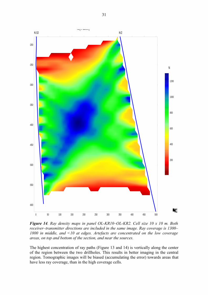
Figure 14. Ray density maps in panel OL-KR10–OL-KR2. Cell size 10 x 10 m. Both

receiver–transmitter directions are included in the same image. Ray coverage is 1300–

1800 in middle, and <10 at edges. Artefacts are concentrated on the low coverage

areas, on top and bottom of the section, and near the sources.

The highest concentration of ray paths (Figure 13 and 14) is vertically along the center

of the region between the two drillholes. This results in better imaging in the central

region. Tomographic images will be biased (accumulating the error) towards areas that

have less ray coverage, than in the high coverage cells.

32

The 3D coordinates of the measurement points are calculated and a correction is made

for the measurement geometry. The normal field is chosen either spherical (inverse

distance) or cylindrical (inverse square–root distance) and source–receiver geometry is

removed (incidence angle compared to dipole axis both from transmitter and to receiver,

Equation 20 above).

A joint analysis of amplitude and phase plots is performed. The above plots are

compared with those of the normal field.

Tomographic inversion is computed to minimise the attenuation integral (21) over the

ray path. Cell size 5 x 5 m was selected for panel OL-KR4 to OL-KR10 and cell size 10

x 10 m for panel OL-KR10 to OL-KR2.

Tomographic processing was performed separately for each frequency, at 312.5, 625

and 1250 kHz for pair OL-KR4–OL-KR10 and at 312.5, 625 kHz for pair OL-KR10–

OL-KR2. At higher frequencies, the signal level was too low, compared to very high

noise level. In a less conductive environment, and in lower noise environment, the high

frequencies would perform well.

Further smoothing of spurious values will perform in the inversion. From the survey

data was removed regions where any geometric or noise interference is distorting the

results, and the transmitter–receiver distance was greater than survey range.

Statistical analysis is used for averaging the attenuation value over rays computed in the

cells. Lowest of obtained absorption coefficients has been used, which is providing the

most robust results.

Each cell has been assigned with a resistivity value. The attenuation between drillholes

is used for estimating the resistivity properties of the rock. The level of resistivity after

inversion has been deduced from external drillhole logging data. Selecting the normal

field and other parameters, it is necessary to have available the resistivity logging data

and the maximum of geological information.

Survey wavelengths range at 50–300 m in Olkiluoto bedrock medium. The wavelength

is much larger in dimension than the thickness of observed features or cell size in

inversion.

Main application scheme of the FARA method is radiowave shadowing, i.e. recognition

of paths where the guided radiowave penetrates well, or does not transmit through. It is

however possible to make amplitude or phase difference imaging using damped

inversion. This would use high measurement coverage, and the cell sizes (5 x 5 or 10 x

10 m here) are not of relevant on their size compared to the wavelength but to the

number of rays penetrating each cell. Creating an image like this may not be

mathematically unique, but it can help in understanding and presenting the

measurement data. Consequently the analysis is not based on wavefield approximation,

and as diffuse field amplitude decay is used, inversion will correspond a straight path

approximation, as curved ray approximation does not have here any physical meaning

like it would for velocity field.

33

With wavelengths 50–300 m the survey is performed in transition domain between near

field and far field. Some precautions are useful when using far field approximation.

In this transition domain several factors affect to the assumed electrical field interaction:

- near–field effects are present, e.g. not only tangential electrical field is

encountered, but also the radial component, which has different polarization and

decay characteristics

- source dipole is not point–like, but has a significant length dimension, here 35

m, compared to target

- actual transmission time is not measured, so there is no control on velocity

- amplitude vs. distance and transmission angle are correlated to resistivity of the

subsurface,

- the changes in phase difference could in principle be associated to dielectric

permittivity, via slowness of the signal

- magnetic permeability is not taken into account in the approximation

- any off–plane events may affect to the actual results, and cannot be resolved in

single–hole survey panel. Several drillhole panels would resolve this case.

- reflection, scattering and diffraction are ignored

- contrasts are assumed small (which is not true in Olkiluoto site).

34

35

6 RESULTS

The interpretations were done with the Russian software. The results with ImageWin

software are presented in GTK Q series report (Korpisalo 2005). Examples of results

obtained by ImageWin are shown for reference of data set not constrained with logging

data. There were 30 appropriate transmitter positions in the first section OL-KR4–OL-

KR10 and 17 positions in the second section OL-KR10–OL-KR2.

A homogeneous resistivity distribution has been taken as a starting value in the

inversion. All additional data including resistivity values in drillholes are taken into

account when tomographic sections are generated. During data handling the Russian

experts represented results which were not constrained with logging data. The images

had the same characteristics as the final images, which are smoother than the images

used in field control.

6.1 Drillhole panel OL-KR4–OL-KR10

For drillhole panel OL-KR4 to OL-KR10 the distance between the drillholes in the

upper part was 250 m, whereas in the lower part of the working interval it was reduced

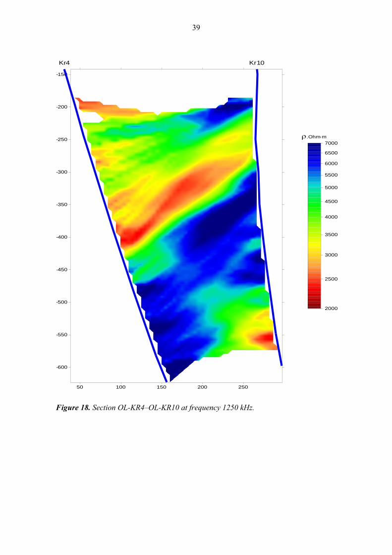
to 150 m. In Figures 15–18, the interpretation results for three frequencies are given.

As a whole, the results obtained at different frequencies coincide. The range of obtained

apparent resistivities is 2000–7000 ohm–m. The contacts of the zones with lower

resistivities are generally dipping from drillhole OL-KR10 to drillhole OL-KR4 (from

the north to the south), the dip angle being about 40 degrees. The main lower resistivity

zone is extended from depths of 220–300 m in drillhole OL-KR10 to depths of 350–430

m in drillhole OL-KR4. The conductivity of this zone increases with depth. No

discontinuity was detected in the crosshole space.

Another lower resistivity zone is adjacent to drillhole OL-KR4 at depths of 220–350 m.

This zone is practically pinched out towards the middle of the crosshole space. A less

intensive and short zone is adjacent to this drillhole at depths of 470–500 m.

Between these conductive zones, there is a resistive layer extending from OL-KR4 at

500–600 m to KR10 at 300–500 m.

All these low resistivity zones are reflected in the available data of resistivity logging.

The sole exception is a lower resistivity zone adjacent to drillhole OL-KR10 at depths

greater than 500 m. The well logs do not show any considerable decrease in resistivity

within this interval; nevertheless, the zone is detected with confidence at all frequencies.

Its appearance may be due to the presence of a conductive zone in the immediate

vicinity of the drillhole both in the tomographic section plane and some distance away

from it. Or, this may result from an error in drillhole deviation profile.

36

50 100 150 200 250

-600

-550

-500

-450

-400

-350

-300

-250

-200

-150

Kr4 Kr10

RIM tomography reconstructionApparent resistivity, 312,5kHz

2000

2500

3000

3500

4000

4500

5000

5500

6000

6500

7000

r.Ohm×m

Figure 15. Section OL-KR4–OL-KR10 resistivity at frequency 312.5 kHz.

37

Figure 16. Attempt to run inversion without drillhole constraint (ImageWin), frequency

312.5 kHz. Red dots are the transmitters. Though it is clear the inversion is not final,

many features are resembling the ones presented by FGUNPP.

38

50 100 150 200 250

-600

-550

-500

-450

-400

-350

-300

-250

-200

-150

Kr4 Kr10

RIM tomography reconstructionApparent resistivity, 625kHz

2000

2500

3000

3500

4000

4500

5000

5500

6000

6500

7000

r.Ohm×m

Figure 17. Section OL-KR4–OL-KR10 at frequency 625 kHz

39

50 100 150 200 250

-600

-550

-500

-450

-400

-350

-300

-250

-200

-150

Kr4 Kr10

RIM tomography reconstructionApparent resistivity, 1250kHz

2000

2500

3000

3500

4000

4500

5000

5500

6000

6500

7000

r.Ohm×m

Figure 18. Section OL-KR4–OL-KR10 at frequency 1250 kHz.

40

6.2 Drillhole panel OL-KR10 – OL-KR2

The distance between the drillholes in the upper part was 300 m, whereas within the

working interval it was 400–500 m. In Figures 19–21, the interpretation results for two

frequencies are given.

The most distinct feature in this drillhole panel is the resistive domain from OL-KR10

at 300–550 m depth level to OL-KR2 at level 200–450 m.

The conditions for measurements in this drillhole pair were less favourable than in the

above mentioned pair. The depth interval of measurements did not exceed 400 m and

was not greater than the distance between the drillholes. Such geometry of does not

allow to obtain the exact contours of boundaries, especially with medium and steep

dips, in the upper and lower parts of the section. Nevertheless, the picture of the central

part of the section is achieved with a sufficient accuracy.

Like in the first drillhole pair, the tomographic sections, obtained at different

frequencies coincide in general. The range of apparent resistivities is within 3000–9000

ohm–m. The conductive zone, adjacent to drillhole OL-KR10 at depths less than 300 m,

is in agreement with the zone obtained in the adjoining section (OL-KR4–OL-KR10). It

is impossible to determine its dip angle because it is too close to the top edge of the

section; one can only assert that this zone goes up towards drillhole OL-KR2 and

intersects it above the studied interval, i.е. above 200 m. The similar situation can be

observed in the bottom part of the section, where a conductive zone is adjacent to

drillhole OL-KR2 and is dipping towards drillhole OL-KR10, going below the studied

interval. The position of this zone is in agreement with the resistivity logging data in

drillhole OL-KR2.

41

0 50 100 150 200 250 300 350 400 450 500

-600

-550

-500

-450

-400

-350

-300

-250

-200

Kr10 Kr2

RIM tomography reconstructionApparent resistivity, 312,5kHz

3000

4000

5000

6000

7000

8000

9000

r.Ohm×m

Figure 19. Section OL-KR10–OL-KR2 resistivity at frequency 312.5 kHz.

42

Figure 20. Section KR10–KR2, an attempt to run inversion without drillhole constraint

(ImageWin), 312.5 kHz. Red dots are the transmitter locations. Though it is clear the

inversion is not final, many features are resembling the ones presented by FGUNPP.

43

Figure 21. Section OL-KR10–OL-KR2 resistivity at frequency 625 kHz.

The dip angles of the lower resistivity zones can be only judged with confidence for the

central part of the section, where an anomalous region is traced adjacent to drillhole

0 50 100 150 200 250 300 350 400 450 500

-600

-550

-500

-450

-400

-350

-300

-250

-200

Kr10 Kr2

RIM tomography reconstruction

Apparent resistivity, 625kHz

3000

4000

5000

6000

7000

8000

9000 r .Ohm × m

Fig. 6

44

OL-KR2 at a depth of about 250 m. Its intensity is decreasing sharply as going away

from the drillhole; however, it can be traced almost to drillhole OL-KR10. Its dip angle

is close to that of the boundaries of conductive regions in the previous pair (about 30–35

degrees). No more marked conductive targets have been detected in the crosshole space.

45

7 COMPARISON WITH DRILLHOLE AND OTHER GEOPHYSICAL DATA

The drillholes intersect mostly migmatitic (veined and diatexitic) gneiss, tonalitic–

granodioritic–granitic gneiss (TGG) and granite pegmatite, which are the dominant rock

types in Olkiluoto (Paulamäki et al. 2006). The bedrock resistivity in DC range varies

according to drillhole logging from highly resistive (> 10 000 ohm.m) gneisses to fairly

conductive sulphide bearing layers (< 100 ohm.m).

FARA data was received in Pöyry Environment Oy as field records and processed

image grids. Field records for each transmitter station and drillhole scan were reviewed

together with drillhole logging data. These recorded values have not been filtered for

spurious values, neither normalized for geometry and distance.

7.1 Reviewing the FARA results 7.1.1 Checking the data against logging

Some general observations were made. From the transmitter antenna, the signal

penetrates generally well to the measurement drillhole. Highest amplitude, or generally

some signal, is found when both receiver and any part of the transmitter are located in a

potentially same, even narrow resistive layer or “window”, if the layer is continuous.

The antennae are long (35 m) compared to intersection length of conductive beds. The

penetration does not depend on antenna length located at the resistive domain.

Resistive layers appear to cause wave guide phenomenon, where the amplitude

increases compared to surroundings. If there are conductive bodies between the

transmitter and receiver, signal will be always decayed. Subsequent conductive layers

(which are typically rather narrow) between the transmitter and receiver will lower the

amplitude step by step with some ratio. When the distance increases, or several layers

are encountered, the signal may decay completely below noise level (e.g from top of

OL-KR4 to bottom of OL-KR10).

One can make some interpretations of the scans even without tomographic image

reconstruction, which would however help in understanding the results geometrically.

Reasonable way to compare the raw data would be to normalize the results for distance

and measurement geometry, and to screen out the outliers with average or median

filtering, and then plot the results along drillhole axis. Here the data was assessed

without normalization.

The compared high amplitude locations, and locations with change of amplitude,

correlate well with the resistivity logging data, and can be explained with drillhole

observations. These results also indicate the possible resistive layer connections

between drillholes, and locations of conductive beds possibly terminating these resistive

domains. It is also possible to estimate the conductive layer locations extending between

the drillholes. General views of the results are presented in Figures 22–25 for profiles

measured from some of the transmitter stations.

46

The results for transmitters in OL-KR4 measured in OL-KR10 are (Figure 22):

- according to amplitude OL-KR4 transmitter locations are on slightly higher

conductivity at 380–440 m, on resistive domain 460 m, and on conductive area

again from 480 m downwards.

- The signal from 200–380 m penetrates to OL-KR10 between 200–260…280 m,

indicating a resistive domain which can be followed. Depth 280–290 m contains

a local conductive body, separating the resistive layers. Source at 380 m “sees”

390 m at OL-KR10 as a blind conductive body.

- The signal penetrates from 400–460 m well to OL-KR10 between 290…330–

450…480 m. Signal level drops upwards from 200 m, and there is a drop in

level also at 230 m. From 480 m in OL-KR4, the signal increases suddenly at

540 in OL-KR10, indicating a resistive connection. Local drop of signal at 400

m indicates presence of a small conductor.

- From 540–600 m in OL-KR4, resistive layer connection is limited between 420–

525…550 m in OL-KR10.

Figure 22. Raw signal from OL-KR4, example stations 200 m, 400 m, 460 m and 600

m, measured in OL-KR10 and long normal resistivity in OL-KR10. Resistivity low areas

in 260–270 m and 290 m and below 400 and 500 m indicate change in amplitude trend.

The reverse measurements from OL-KR10 sources in OL-KR4 indicate rather similar

behaviour (Figure 23):

- Sources at 210 and 250 m suggest a resistive layer to continue until ca. 400 m in

OL-KR4, where are found some conductive bodies.

- Source at 290 m indicate almost step–like feature, with limits of high amplitude

domain, or shadowing up and downwards, at 300 and 450 m. This zone, despite

of high amplitude, is a conductive domain in logging, which would suggest the

high amplitude is caused by guided wave.

47

- Sources at 330–410 m show resistive layer connection to 430–490 m in OL-

KR4, and sources 450–570 m connection to below 530 m. For these sources the

300–450 m in OL-KR4 indicates lower resistivity than sections below and

above, indicating also a strong conductor domain in reconstructed resistivity

images. It can be suggested that conductor domain between OL-KR4 300–450 m

and OL-KR10 260–290 m, seen also in resistivity logging, is continuous through

the drillhole section.


m, measured in OL-KR4 and long normal resistivity in OL-KR4. Resistivity low areas

in 300–430 m and 490 m indicate change in amplitude trend.

The profiles measured in OL-KR2 from transmitters in OL-KR10 indicate rather

interesting behavior (Figure 24):

- Transmitters at 210 and 250 m in OL-KR2 indicate very low amplitude, though

closest distance between drillholes. This is apparently due to conductors at 260–

270 m and 290 m in OL-KR10, which is not penetrated by the measurement

system. For all other profiles, these conductors are seen as amplitude change at

250–280 m.

- A resistive layer is seen from all transmitters 290–570 m in OL-KR10 at 280–

400 m in OL-KR2. This is matching with long normal resistivity logging data.

Depths 530 m and 600 m indicate also amplitude drop (possible conductors) in

OL-KR2.

The profiles measured in OL-KR10 from transmitters in OL-KR2 show following

(Figure 25):

- Practically very little signal reaches OL-KR10 from deep parts of OL-KR2

below 560 m. Drillholes are deviated away from each other.

48

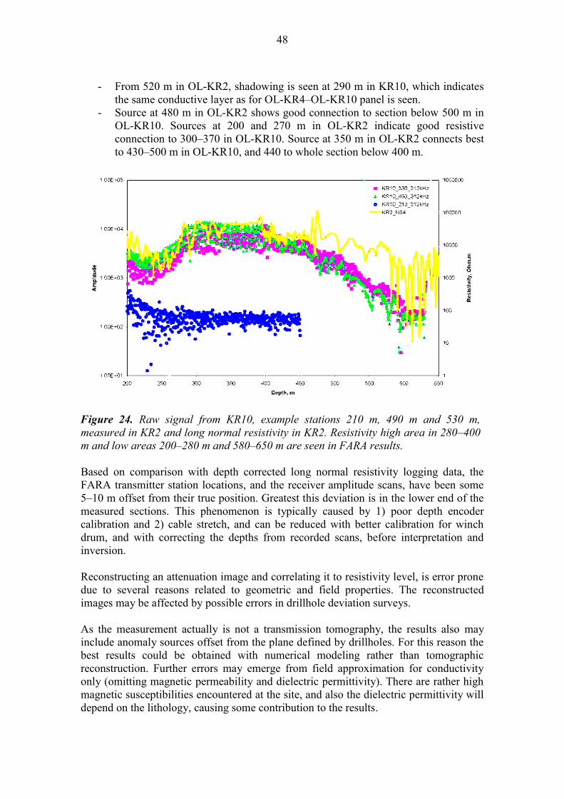
- From 520 m in OL-KR2, shadowing is seen at 290 m in KR10, which indicates

the same conductive layer as for OL-KR4–OL-KR10 panel is seen.

- Source at 480 m in OL-KR2 shows good connection to section below 500 m in

OL-KR10. Sources at 200 and 270 m in OL-KR2 indicate good resistive

connection to 300–370 in OL-KR10. Source at 350 m in OL-KR2 connects best

to 430–500 m in OL-KR10, and 440 to whole section below 400 m.

Figure 24. Raw signal from KR10, example stations 210 m, 490 m and 530 m,

measured in KR2 and long normal resistivity in KR2. Resistivity high area in 280–400

m and low areas 200–280 m and 580–650 m are seen in FARA results.

Based on comparison with depth corrected long normal resistivity logging data, the

FARA transmitter station locations, and the receiver amplitude scans, have been some

5–10 m offset from their true position. Greatest this deviation is in the lower end of the

measured sections. This phenomenon is typically caused by 1) poor depth encoder

calibration and 2) cable stretch, and can be reduced with better calibration for winch

drum, and with correcting the depths from recorded scans, before interpretation and

inversion.

Reconstructing an attenuation image and correlating it to resistivity level, is error prone

due to several reasons related to geometric and field properties. The reconstructed

images may be affected by possible errors in drillhole deviation surveys.

As the measurement actually is not a transmission tomography, the results also may

include anomaly sources offset from the plane defined by drillholes. For this reason the

best results could be obtained with numerical modeling rather than tomographic

reconstruction. Further errors may emerge from field approximation for conductivity

only (omitting magnetic permeability and dielectric permittivity). There are rather high

magnetic susceptibilities encountered at the site, and also the dielectric permittivity will

depend on the lithology, causing some contribution to the results.

49


m, measured in OL-KR10 and long normal resistivity in OL-KR10. Resistivity low area

in 260–290 m and high below 300 m is seen in FARA results.

Image reconstruction in FGUNPP used the drillhole electrical logging data as

constraint. Attempt to reproduce the inversion using ImageWIN software in GTK led to

a roughly similar resistive and conductive domain distribution as in FGNUPP images,

but more spurious and scattered images, so apparently stronger smoothing is necessary.

Drillhole resistivity constrain has not been possible in GTK approach. Some crossing X-

shaped lines over the image panel suggest that the drillhole geometry, or depth levels of

measurement stations, are not correct.

The transmitter locations indicate bulls–eye type increase in conductivity. Emphasis

should be made to reject spurious values, select a proper inversion scheme from

available options (between ART, SIRT, Conjugate gradient or Least squares), select

efficient averaging and damping methods, and to select a proper, large enough cell size.

Results are reasonable to display on a narrow amplitude scale, to prevent spurious

extreme values from dominating the images.

Apparently the FGUNPP inversion has managed to use a robust technique in averaging

the decay values on cells (selection has been made to use minimum attenuation). Trade

off of using logging data is the expected tendency to satisfy the logging information,

and generate errors elsewhere. The images are increasing conductivity levels in areas

where coverage of data is reduced, and emphasizing the continuity of resistive and

conductive features from drillhole to another.

It would be useful to compute and display the inversion both without any drillhole

resistivity constrain data used, and with constrain applied. Backward comparison was

50

made between drillhole logging data and cell resistivity values picked from images. A

reasonable match is natural as drillhole resistivities have been used (Figure 26).

Resistivities obtained from image are smoother, varying less than logging data.

Nevertheless it is possible to locate some coinciding resistive and conductive domains

along drillholes.

51

a)

b)

Figure 26. Picked cell resistivities on vertical depth from FARA image of 312.5 kHz, a)

OL-KR4 and b) OL-KR10. The FARA resistivities are smoother, and slightly below the

DC resistivity values. Higher conductivity in KR4 is clearly observed. Minima are

close to same locations, but not perfectly, indicating possible depth errors. With

increasing depth, FARA resistivity gets lower, which may indicate error in deviation

profile, or e.g. influence of saline groundwater in bedrock.

52

7.1.2 Internal consistency of FARA tomograms

The FARA tomograms were compared between frequencies 312.5 kHz, 625 kHz and

1250 kHz, and between drillhole sections OL-KR4–OL-KR10 and OL-KR10–OL-KR2.

Images were displayed on a same resistivity scale between all frequencies and both

panels to allow comparison. There is a distinct resemblance of results between the

frequencies, though there are more details on higher frequencies.

On a general view the reconstructed image panels coincide, as compared to each other

at their seam location along OL-KR10. The match is partly good and partly poor. The

resistivity levels range from 2000–3000 to 7000–9000 Ohm–m in the panels, drillhole

OL-KR10–OL-KR2 indicating a slightly higher resistivity than OL-KR4–OL-KR10

(either a real property or a leveling error).

Conductive and resistive beds, and their potential orientations (southerly dips) are

matching fairly well to estimated geological control. Images suggest a strong

continuation of features dipping from right (North) to left (South) downwards at 20–30

degrees apparent dip in both panels OL-KR4–OL-KR10 and OL-KR10–OL-KR2.

Inversion without drillhole constraint does not emphasize so much the conductor

continuity between drillholes (Figures 16 and 20 above).

Well matching part is the 200–400 m interval in OL-KR10, where the conductive

locations at 250–300 m appear well in both panels. The panel OL-KR4–OL-KR10

suggest conductive zone residing near the upper part of OL-KR4, and possibly

continuing towards upper part of OL-KR10. Upper part of OL-KR10–OL-KR2 panel

indicates conductive domain on the top of the section.

Also the continuous resistive domain between lower part of OL-KR4 to mid–OL-KR10

at 300–400 m is seen in OL-KR10 all results. This domain is extending through panel

OL-KR10–OL-KR2 to pass through OL-KR14 and to reach OL-KR2.

Further the results suggest that there is a high conductivity adjacent to deepest part of

OL-KR10 at 450–600 m in OL-KR4–OL-KR10 panel. This does not receive support

from drillhole logging data. The resistivity in OL-KR10–OL-KR2 panel is high at this

location, receiving gain from the logging data.

Possible reasons for the contradiction are a real conductive zone somewhere near OL-

KR10 (increased sulphide content or saline groundwater boundary), or an error in

drillhole deviation file, causing failure in field normalization. This may also appear an

inversion artefact due to low data density.

Nevertheless there is a conductive domain between the lower part of OL-KR2 and OL-

KR10, which may be seen in OL-KR2 but not penetrated by OL-KR10.

53

Figure 27. Drillhole resistivity images OL-KR4, OL-KR10, OL-KR14 and OL-KR2 with

FARA tomograms of 312.5 kHz (resistivity range 2000–8000 ohm–m) and long normal

resistivity (blue) and fracture frequency (orange) logging profiles.

54

Reasons to contradiction may range:

a) unknown conductive body between OL-KR4–OL-KR10 or close to OL-

KR10 at 450–550 depth range, not intersected in any of drillholes

b) a large unconformity in otherwise continuous structure near KR10

(fault, fold,….)

c) noise or error in measurement data at this depth range

d) error in level of the data (e.g. the source intensity)

d) artefact on inverted image due to limited amount of ray density and

unfavourable geometry, when in inversion the errors would spread to less

covered areas.

These issues may become resolved during further investigations, like imaging between

other nearby drillhole pairs, or recomputing the tomographic reconstruction with

updated drillhole deviation data.

The resistivity images on different frequencies are displayed in Figures 27–30, along

with rock types and fracture frequency, and rendered resistivity distribution in drillhole

logging on same resistivity scale.

55

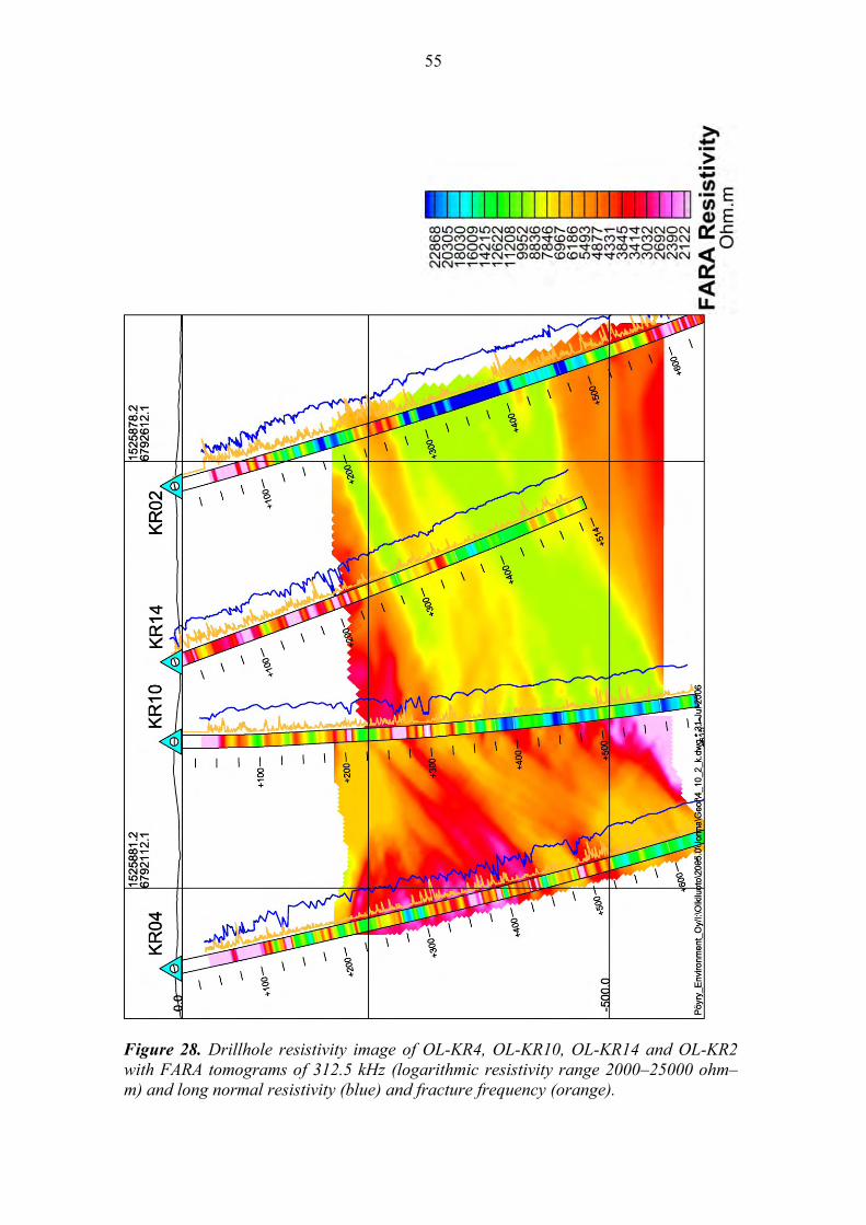
Figure 28. Drillhole resistivity image of OL-KR4, OL-KR10, OL-KR14 and OL-KR2

with FARA tomograms of 312.5 kHz (logarithmic resistivity range 2000–25000 ohm–

m) and long normal resistivity (blue) and fracture frequency (orange).

56

Figure 29. FARA tomograms of 625 kHz and drillhole resistivity images (in

logarithmic resistivity from 2000 to 8000 ohm.m, see Figure 27 for legend), along with

profiles long normal resistivity (blue) and fracture frequency (orange).

57

Figure 30. FARA tomogram of 1250 kHz (OL-KR4–OL-KR10) and drillhole resistivity

images (logarithmic resistivity range 2000–8000 ohm–m, legend in Figure 27), with

long normal resistivity (blue) and fracture frequency (orange).

58

7.2 Comparison of FARA results to other data

The FARA images were drawn on vertical section Easting = 1526.000 (Finnish KKJ1)

in 3D visualization CAD system at uniform resistivity scales, together with drillholes,

lithology, drillhole fracture frequency (Paulamäki et al. 2006), electrical long normal

resistivity logging, magnetic susceptibility, sonic P–velocity (Julkunen et al. 1995, Lahti

et al. 2001, Laurila & Tammenmaa 1996, SMOY 1989, SMOY 1990), radar single hole

attenuation and first arrival time (Carlsten 1990, 1991, 1996a, b; Saksa et al. 2001), and

the seismic velocity tomogram from OL-KR4–OL-KR10, and a migrated crosshole

seismic reflection map at Z: -120– -600 m, the large scale seismic VSP reflectors

(Enescu et al. 2004, Heikkinen et al. 2004a), and geological structures and deformation

zone intersections from geological model version 0 (Paulamäki et al. 2006).

To compare the results to the other available electrical results, also large scale

electromagnetic and electrical results were shown. The frequency domain

electromagnetic Gefinex 400 Sampo sounding (vertical magnetic dipole) interpretations

from 200 m in-line profile (Paananen et al. 2007, Paulamäki et al. 2006), and pole-pole

electrical soundings (Heikkinen et al. 2004b) were plotted on the vertical section.

Results of crosshole mise-á-la-massé survey were presented (Lehtonen 2006).

These were used to correlate the other geophysical information from the vertical section

to FARA results.

7.2.1 Comparisons to drillhole results

Drillhole data can be compared in OL-KR4 at 200–650 m, OL-KR10 200–575 m, OL-

KR14 220–514 m and OL-KR2 190–600 m where tomographic images and drillhole

data overlap. Tables 3-6 below represent the observations.

The reported rock types of drillhole include different varieties of migmatitic gneisses

and pegmatite granite (Figure 31). Resistivity is associated on the other hand to FARA

results, and on the other hand together with susceptibility to sulphide content, texture,

and lithology.

Most important correlation of tomogram features is expected to associate with

resistivity logging data. Also the radar velocity and amplitude attenuation are

correlating to these locations. It is known that conductive zones are linked also to higher

susceptibility in Olkiluoto (sulphide minerals). In some cases there are connections of

conductivity in the tomogram to the acoustic logging data, and this way possibly to

density, which are on the other hand directly linked to seismic reflection data. Lower

density values are usually associated to pegmatite veins, but in some cases also narrow

distinct fracture zones.

59

Table 3. Comparison of tomographic reconstruction to OL-KR4 data.

Depth

section

in OL-

KR4

FARA

observation

Lithology Deformation Geophysical logging

200-330 Conductive DGN Fracturing

associated to

conductivity.

BFZ at 315 m.

Dominant

orientations

gentle.

Conductive, not magnetic. At

200-280 m low radar amplitude

and velocity. Narrow sections of

acoustic velocity minima (310-

320), possible reflectors.

330-450 Conductive MGN,

small

DGN, PGR

and VGN

parts

Fracturing

associated to

conductivity.

Dominant

orientations

gentle.

Conductive.

Magnetic.

Higher density.

Very low radar velocity and

amplitude.

Narrow sections of acoustic

velocity minima (370-380).

Increasing salinity indicated in

fluid resistivity.

450-490 Resistive VGN,

partly PGR

Dips gentle to

east. Increased

fracturing

increases the

conductivity only

slightly.

Hydraulic

conductivity.

Resistive. High radar velocity

and amplitude.

490-495 Conductive VGN,

partly PGR

Sulphides. Conductive. Magnetic.

Radar attenuation.

.

495-530 Conductive VGN,

partly PGR

Pervasive

kaolinite and illite

alteration, steep

dips to SW.

Slighly decreased resistivity.

Radar attenuation. Distinct

sonic velocity minimum at 510-

530 m, possible reflector

530-650 Resistive VGN,

partly PGR

Moderate, steep

dips to S-SE.

Fracture

frequency and

conductivity

poorly associated.

Resistive. Radar amplitude and

velocity high (110-120 m/µs).

Minor conductive locations

seen, alternating sonic velocities

at 570-620 m

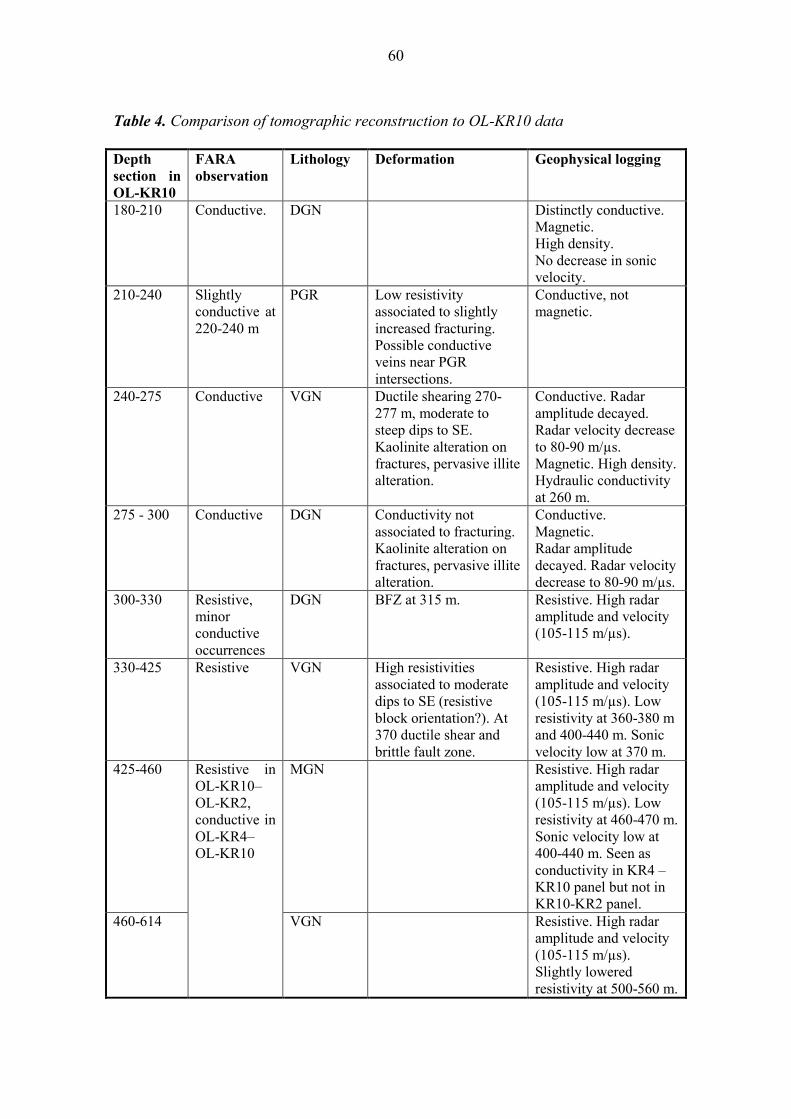
60

Table 4. Comparison of tomographic reconstruction to OL-KR10 data

Depth

section in

OL-KR10

FARA

observation


180-210 Conductive. DGN Distinctly conductive.

Magnetic.

High density.

No decrease in sonic

velocity.

210-240 Slightly

conductive at

220-240 m

PGR Low resistivity

associated to slightly

increased fracturing.

Possible conductive

veins near PGR

intersections.

Conductive, not

magnetic.

240-275 Conductive VGN Ductile shearing 270-

277 m, moderate to

steep dips to SE.

Kaolinite alteration on

fractures, pervasive illite

alteration.

Conductive. Radar

amplitude decayed.

Radar velocity decrease

to 80-90 m/µs.

Magnetic. High density.

Hydraulic conductivity

at 260 m.

275 - 300 Conductive DGN Conductivity not

associated to fracturing.

Kaolinite alteration on

fractures, pervasive illite

alteration.

Conductive.

Magnetic.

Radar amplitude

decayed. Radar velocity

decrease to 80-90 m/µs.

300-330 Resistive,

minor

conductive

occurrences

DGN BFZ at 315 m. Resistive. High radar

amplitude and velocity

(105-115 m/µs).

330-425 Resistive VGN High resistivities

associated to moderate

dips to SE (resistive

block orientation?). At

370 ductile shear and

brittle fault zone.

Resistive. High radar


(105-115 m/µs). Low

resistivity at 360-380 m

and 400-440 m. Sonic

velocity low at 370 m.

425-460 Resistive in

OL-KR10–

OL-KR2,

conductive in

OL-KR4–

OL-KR10

MGN Resistive. High radar


(105-115 m/µs). Low

resistivity at 460-470 m.

Sonic velocity low at

400-440 m. Seen as

conductivity in KR4 –

KR10 panel but not in

KR10-KR2 panel.

460-614 VGN Resistive. High radar


(105-115 m/µs).

Slightly lowered

resistivity at 500-560 m.

61

Table 5. Comparison of tomographic reconstruction to OL-KR14 data (radar not

measured; FARA measurement did not use OL-KR14).

Depth

section in

OL-KR4

FARA

observation

Lithology Deformation Geophysical

logging

220-275 Conductive VGN Conductivity not

associated to fracturing,

unless associated to 185

m zone.

Conductive,

several narrow

layers. Magnetic.

High density. No

significant sonic

anomalies.

275-325 Resistive, slight

decrease.

PGR Moderate dips to south.

slight increase in

fracturing. Hydraulic

conductivity.

Resistive.

325-350 Resistive VGN Fractured, illite and

kaolinite on fractures.

Resistive. Minor

conductive

indication at 320-

340 m. Low sonic

velocity. Low

density. Low

susceptibility.

350 Slightly

decreased

resistivity

MFGN Not associated to

fracturing.

Resistive

350-370 Resistive PGR Moderate dips to SE,

possible orientation of

resistive block.

Below 440 m brittle

faults, kaolinite and

illite on fractures.

Resistive. Below

440 m slight

decrease in sonic

and resistivity, not

seen in tomogram.

370-440 Very resistive TGG

440-514 Resistive VGN/PGR

62

Figure 31. Drillhole OL-KR4, OL-KR10, OL-KR14 and OL-KR2 lithological profiles,

along with FARA tomographic images of 625 kHz, long normal resistivity and

susceptibility. For resistivity legend, see Figure 27.

63

Table 6. Comparison of tomographic reconstruction to OL-KR2 data.

Depth

section in

OL-KR2

FARA

observation


190-215 Resistive VGN Moderately

fractured.

Resistive. Sligthly

reduced sonic velocity

and radar amplitude.

215-250 Conductive MGN/PGR Increased fractur-

ing, pervasive

kaolinite alteration,

few BFZs.

Orientations gentle-

moderate to S-SW.

Wide minimum in

resistivity and sonic

velocity. May associate

to VSP reflector. Radar

amplitude reduced.

250-300 Resistive VGN/DGN Non fractured.

Foliation 40-50

degs to south,

possible orientation

of resistive block.

Very resistive. Radar

velocity minimum at

260 m. Low

susceptibility. High

sonic velocity. Small

zone at 290 m.

300-400 Very resistive.

Minor decrease

at 290-330 m.

TGG Very resistive. Small

zones at 315 and 330 m.

Distinct and continuous

radar reflector at bottom

of the section (mafic

vein at 393 m).

400-425 Resistive VGN Slightly increased

fracturing, gentle

dips.

Resistive, resistivity,

radar amplitude and

sonic velocity

alternating. 425-450 Slight increase in

conductivity.

PGR Illite alteration on

fractures.

450-510 Resistivity

decreases in

tomogram

VGN Locally fracture

frequency in-

creased. Moderate

dips. 467-473 m

DSZ and 481-483

BFZ, pervasive

illite alteration,

BFZ at 504-508 m.

below 510 Increasingly

conductive

DGN Fracturing

increased. At 597-

622 m kaolinite

alteration on

fractures, pervasive

illite alteration,

BFZ at 600-605 m.

Resistivity lowered,

possibly salinity

increases. Susceptibility

increases.

below 580 increasingly

conductive

DGN Conductivity increased.

Susceptibility increased.

Radar velocity and

amplitude decreased.

Sonic velocity

decreased.

64

The reason for high resistivities in OL-KR10–OL-KR2 interval is the tonalitic–

granodioritic–granitic gneiss. The diatexitic and mica gneisses indicate slightly lower

resistivities. The apparent dip of resistive region follows this rock type section and can

be confirmed rather continuous on this basis.

Southward of OL-KR10 the associated rock types changes. Tonalitic–granodioritic–

granitic gneiss is not reported in OL-KR4 and OL-KR10 in greater extents. Between

OL-KR10–OL-KR14 high resistivity is more associated to veined gneiss, and increase

of conductivity may be associated to mica gneiss and diatexitic gneiss occurrences.

Apparent southerly dip of resistive body is maintained. Between OL-KR4–OL-KR10

the same trend is emphasized, but dip of resistive body is steeper in dip. Conductive

rock mass is more associated to mica gneiss and diatexitic gneiss.

Increased fracturing and a ductile shear zone (moderate dips to south) at 490–540 m

cannot be seen at all in OL-KR2–OL-KR10 panel, but apparently is associated to local

higher conductivity in panel OL-KR4–OL-KR10. So apparently this feature has

continuity, or shadowing effect, towards OL-KR4 but not towards OL-KR2.

On general view, resistive blocks do not contain major fracturing domains. Normally

increased fracturing can be seen as slightly increased conductivity, and in some cases as

reported brittle faults (Figure 33, Paulamäki et al 2006). Higher conductivity apparently

is related to larger domains of increased fracturing, but there may be also other reasons

associated to conductivity increase than fractures. These indications may sometimes

associate to ductile shearing.

In OL-KR4, drillhole fluid salinity, and fracture groundwater salinity, start to increase

below 320 m, but apparently this feature cannot be seen in FARA tomogram in OL-

KR4.

65


along with FARA tomographic images of 625 kHz, long normal resistivity and fracture

frequency. OL-KR14 resistivity data seems to have a good correlation on resistivity with

FARA image (drillhole has not been involved in the survey, nor used as constrain).

66

Figure 33. The FARA tomogram of 312.5 kHz, resistivity logging profile, and

geological structure intersections, on the vertical cross section. Some of the gently

dipping zones have a similar apparent trend on the plane as the resistive layer limits

have.

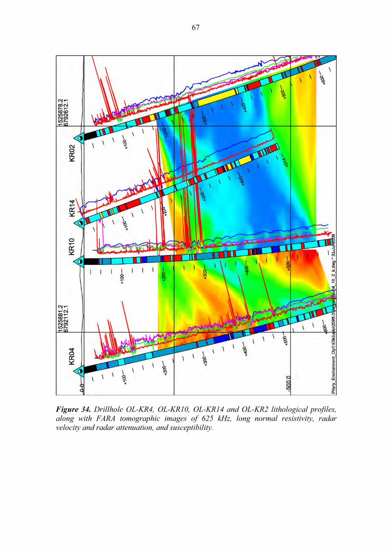
67


along with FARA tomographic images of 625 kHz, long normal resistivity, radar

velocity and radar attenuation, and susceptibility.

68


along with FARA tomographic images of 625 kHz, fracture frequency, gamma–gamma

density and P–wave velocity.

69

7.2.2 Comparisons to electromagnetic sounding results

The electromagnetic SAMPO frequency soundings were performed on ground surface

and interpreted as series of 1D inversion. The rendered image of adjacent inversions (50

m interval) display the upper contact depth for the first distinct conductive layers. The

match of the conductive body at upper part of FARA images and drillhole data shows a

good correspondence.

Figure 36. SAMPO apparent resistivity section from 1–D interpretations of 1995.

Image displays also resistivity regions in FARA image for above 6500–8000 ohm–m

(blue) and below 3000–4000 ohm–m (red), and long normal resistivity images and

curves from drillholes.

70

A cross section submitted by Turo Ahokas, based on interpretations on 1995, will

display at depth level from 200 m in OL-KR4 to 100 m in OL-KR14 a dipping

conductive body, below which one cannot make interpretation with 200 m transmitter–

receiver separation. Upper surface of conductor dips at moderate dip values towards

south.

Figure 37. SAMPO apparent resistivity section from 1–D interpretations of 2005.




71

Towards south, it seems that the conductive body is located upper, being met at some

60–80 m in OL-KR4, as supported by OL-KR4 logging data. Below this layer there

seems to be fairly resistive material on cross section, which should be checked from

other drillholes. Towards north from OL-KR14, higher resistivity at deeper parts of OL-

KR14 seems justified from EM sounding data, and again the sounding stations near OL-

KR2 indicate a strong conductor at 200–210 m supported by logging data, below which

there is no opportunity to investigate using this system.

A revised line interpretation (Paananen et al. 2007) included into electrical model of

Olkiluoto, diplays a more precise location data of the conductive layers. Drillhole data

and resistivity level information have been used in interpretation. The thicknesses of

layers might need to be set narrower. Using drillhole constrains, there can be seen a

layer at 80–120 m depth in KR4 region and south of it, which is horizontal in the

section, or slightly tilting towards the north. The layer steeply bends downwards

between OL-KR4–OL-KR10, being met at 250–300 m depth level in OL-KR10. Then at

300–500 m depth level there are conductors again in OL-KR4, and between these two, a

resistive block. Between OL-KR10 and OL-KR14 the layer from OL-KR10 at 300 m

would reach towards depth OL-200 m in OL-KR14, but on the other hand, some

indications towards northerly dips are still present between OL-KR14 and OL-KR2. A

layer of higher conductivity can be seen in OL-KR2 at 40–120 m, matching well with

drillhole data. FARA images between OL-KR4–OL-KR10 and OL-KR10–OL-KR2 do

not start before a depth of 200 m, but they seem to suggest clearly a bit more southward

dipping structure in the area (except at upper part of OL-KR4, where SAMPO image is

close to FARA result, too). Upper of these SAMPO conductive layers actually is not

imaged until from below the structure, as it is not possible to make measurements closer

to the surface. The apparent difference between the recent SAMPO interpretation and

FARA results could use e.g. drillhole lithology orientation data to resolve. Electrical

model of Olkiluoto (Paananen et al. 2007) would suggest there is a domain containing

conductors in the surface layer, with lower contact dipping moderately (20-40 degrees)

to south, and a rather thick > 200 m resistive (non-conductor containing) domain below

it. Again below this resistive domain, there are conductive layers. This phenomenon is

fully supported by FARA results, confirming the continuity of resistive material

between the drillhole intersections. Also the geophysical model objects merged from

mise-á-la-masse, ground EM, SAMPO and drillhole logging, suggest the FARA data is

fairly consistent.

7.2.3 Comparisons to electrical pole–pole sounding results

Electrical pole–pole soundings were performed on the ground surface and interpreted as

2–D inversion. The interpretation applied the drillhole logging data as constrains, and is

presenting the rather coarse resistivity distribution to a maximum depth of 250–300 m.

Increased conductivity in a layer close to the ground surface (0…80 m) can be seen

from the data. Below that, at 50…150 m level, there is a slightly more resistive region.

The upper surface of more conductive layers at some 200–300 m level can be seen in

results very coarsely, which in turn are seen from below in FARA images. The

conductivity met in OL-KR10 and OL-KR14, and partly in OL-KR2, will support that

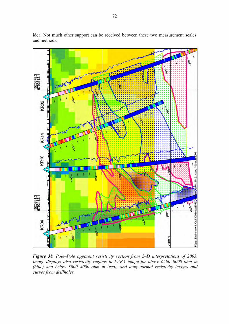
72

idea. Not much other support can be received between these two measurement scales

and methods.

Figure 38. Pole–Pole apparent resistivity section from 2–D interpretations of 2003.




73

7.2.4 Comparison to Mise á la masse results

The results from OL-KR4 mise a la masse current earthing (368 m) potential rendered

from OL-KR24, OL-KR37, OL-KR4, OL-KR30, OL-KR14 and OL-KR2 on same

profile, some interesting results emerge.

Figure 39. a) Mise á la masse image from OL-KR4, 368 m current earthing, b) the

same image added with FARA tomograms (312.5 kHz). Results are clearly of same

origin. FARA is more detailed and will set emphasis for resistive domains, too.

74

The MAM image is fairly smooth, indicating well the domain where the current is

concentrated. FARA would support this image by showing where the resistive domains

are located, and displaying potential conductive locations as shadowing effect locations,

or conductive regions in the tomographic image. Methods are supplementing each other.

7.2.5 Comparison to seismic crosshole tomography and reflector model

The seismic tomogram of OL-KR4–OL-KR10 interval is averaging the evidently

narrow occurrences of low velocities to a rather limited range of velocity variation, just

some 100 m/s below general 5720–5760 m/s level (Figure 40). The velocity minima in

sonic logging fit well together to tomogram (Heikkinen et al. 2004), and the low

velocity zones indicate well also the apparent orientations of the weakness or fracturing

zones.

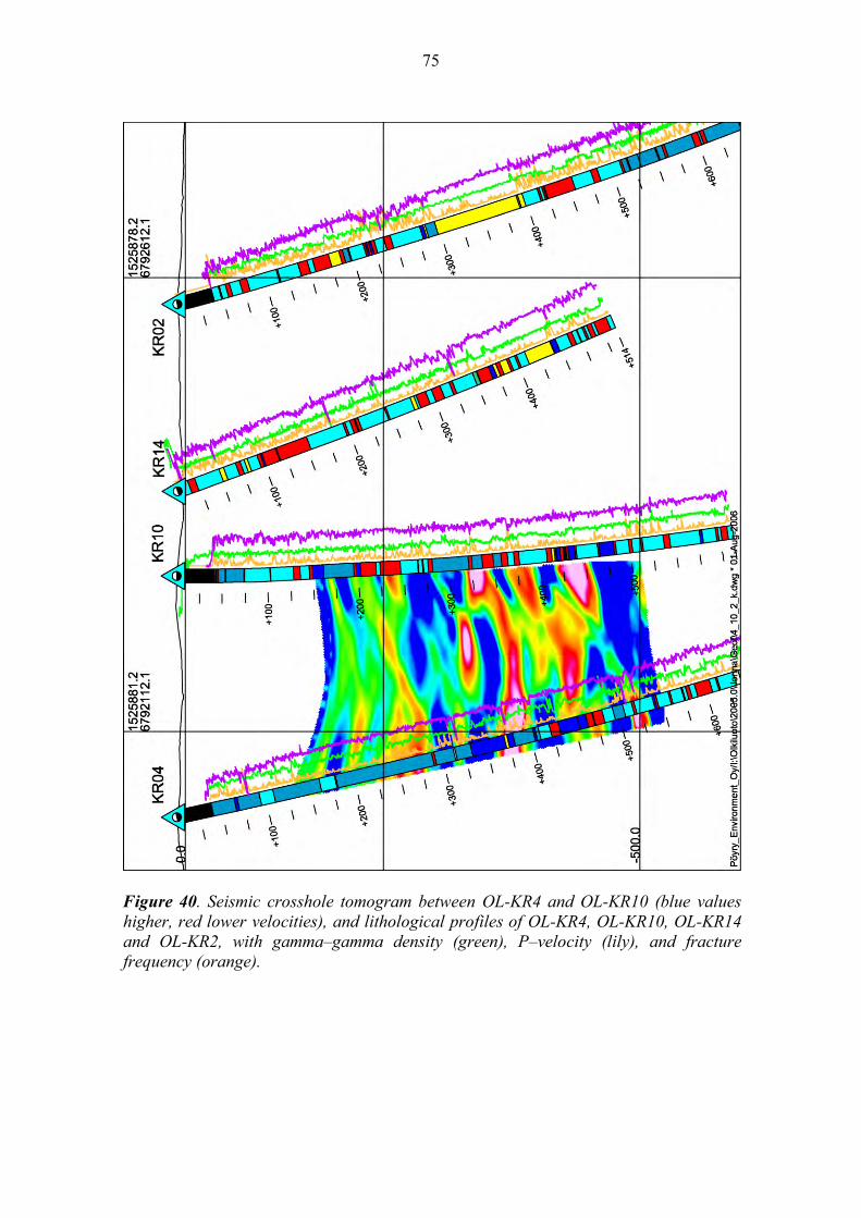
75

Figure 40. Seismic crosshole tomogram between OL-KR4 and OL-KR10 (blue values

higher, red lower velocities), and lithological profiles of OL-KR4, OL-KR10, OL-KR14

and OL-KR2, with gamma–gamma density (green), P–velocity (lily), and fracture

frequency (orange).

76

Figure 41. Seismic 3-D migrated crosshole reflection map from OL-KR4 to OL-KR10,

and lithological profiles of OL-KR4, OL-KR10, OL-KR14 and OL-KR2, with long

normal resistivity (blue), gamma-gamma density (green), P-velocity (lily), and fracture

frequency (orange).

The resistive blocks or their contacts to conductive regions do not fully associate to

seismic low velocity zones or VSP reflectors. Inside the conductive and resistive

regions, there appear slightly differently oriented, cross cutting, and much narrower low

velocity zones, and reflecting surfaces.

77

Between OL-KR4–OL-KR10 the upper contact of resistive body indicates apparent dip

of 30–40 degrees to South. This is supported by a set of VSP reflectors dipping

moderately–steeply to the east (Figure 44). Contrary to this, uppermost low velocity

zone at 350 m depth level has a dip of 12–15 degrees, supported by gently to southeast

dipping reflectors (Figure 45). This set of reflectors support well the gentle dip of upper

contact on tonalite–granodiorite–granite gneiss between OL-KR10–OL-KR14–OL-KR2.

Below this low velocity zone there is a patchy series of zones at steeper apparent dip,

which match better to the resistive area (OL-KR4 at 500 m to KR10 at 350 m), and gets

also support from steeply to southeast dipping features.

Two of the most visible low velocity zones are intersecting the conductive region, and

there is also a higher velocity domain within the conductive zone. At 250 m depth

range, a low velocity zone may coincide with more gently dipping higher conductivity

zone. A low velocity zone at 400–420 m depth level intersects the resistive body at

gentle dip. In some cases these low velocity zones and associated reflectors are seen as

weak and more local low resistivity regions on the FARA tomograms.

The VSP reflectors match well with their orientations to the low velocity zones. There

are some indirect suggestions on displacements (possible subvertical faults) on the

velocity and FARA tomograms. These may receive further support from subvertical

VSP and crosshole reflectors in this drillhole panel.

The subvertical reflection indications (Figure 42) especially towards the west may also

explain the highly variable character of OL-KR4–OL-KR10 and OL-KR10–OL-KR2

drillhole panels in FARA imaging near bottom part of OL-KR10, as well as bending or

terminating conductivity features in FARA results.

78

Figure 42. The FARA tomogram of 625 kHz, velocities in seismic tomogram above

5760 m/s (blue) and below 5730 m/s (red), and possible vertical faulting on basis of

FARA resistivity images and seismic crosshole tomogram. Drillhole lithological profile,

and resistivity, velocity, density and fracture frequency profiles are also shown. Higher

velocity seems to associate to low resistivity. The dips of the velocity variation zones are

more gentle than the resistivity zones.

79

Figure 43. The FARA tomogram of 312.5 kHz, drillhole resistivity images, resistivity

logging profile, and subvertical VSP reflectors dipping to the southwest–west, on the

vertical cross section. These reflectors may represent potential faulting events for

resistivity gently dipping zones.

80


logging profile, and subvertical VSP reflectors dipping to the east or southeast, on the

vertical cross section.

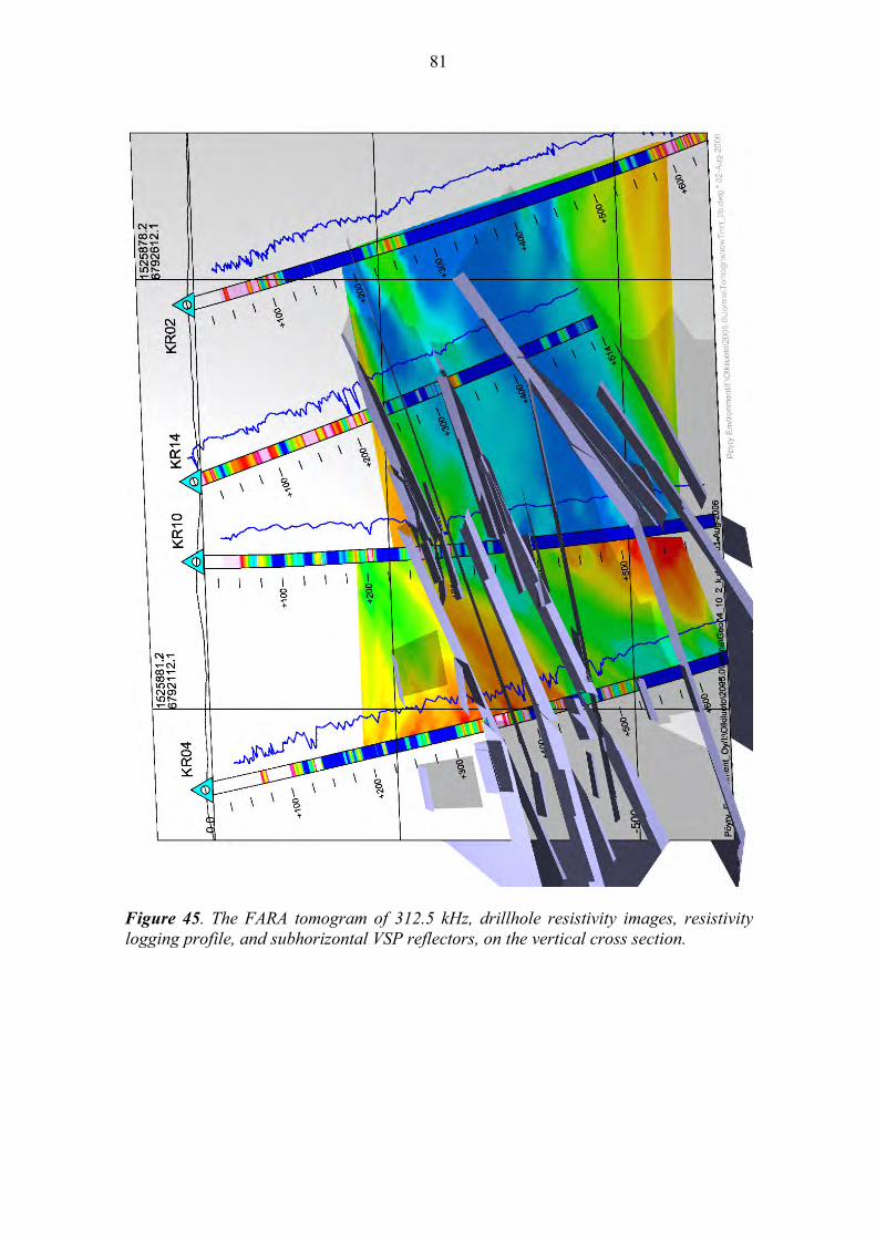
81


logging profile, and subhorizontal VSP reflectors, on the vertical cross section.

82

83

8 DISCUSSION

In October–November 2005, a group of specialists of the FGUNPP «Geologorazvedka»

jointly with the GTK have carried out FARA radio wave imaging in the Olkiluoto site.

Two adjacent drillhole pairs (OL-KR4–OL-KR10 and OL-KR10–OL-KR2) were

surveyed at depth interval of 200–600 m.

The method uses a full space approximation of electrical dipole field. The resistivity,

100–10000 Ohm.m, and frequency range 312.5–2500 kHz defines the field properties

apply in low Q domain (inverse loss tangent), i.e., diffuse or transition domain rather

than a propagating wave field, which makes some challenges in understanding the

results. For electrical dipole field, survey operates in sense of wavenumber vs. drillhole

distance range in intermediate to far field domain. For this reason the tangential

electrical component can be applied, and fair approximation of linear attenuation over

distance is made for computing tomographic reconstruction. Attenuation is correlated

well to electrical conductivity in this transition domain between diffuse and propagating

field. Linearity of attenuation, and geometric concerns of diffuse field detecting also off

plane conductors, need to be taken into account in interpretation.

Processing and preliminary interpretation of the measurement results were performed

during 1–2 days after their completion, the results being given in the present report. The

presence of some lower resistivity zones, and a resistive domain, in the crosshole space

has been detected, and their apparent shape and orientation in the sections were defined.

The positions of the targets, obtained in the two tomographic sections, are in agreement

with each other.

The measurement geometry was not optimal for full tomographic survey resulting from

long distances between the drillholes and too short winch cables limiting the depth of

scan. Now the maximum survey depth was restricted to 600 meters. Longer cables

should have made it possible to detect deeper parts of the drillholes.

It should had been better to use much shorter transmitter step size ( 5 m) so the ray

density would have become higher and the resolution better. Also shorter steps size

would have offered an excellent possibility to investigate the function of the step size to

the reconstruction of the drillhole sections. Simultaneously it could have been possible

to consider the effects of different cell sizes better. Higher transmitter density would

also help in rejecting of spurious data.

Lower two frequencies, 312.5 kHz and 625 kHz can be applied to drillhole distances of

400–500 m in the area. The higher 1250 kHz frequency can be used at distances 200–

300 m, but the highest 2500 kHz does not penetrate through in Olkiluoto moderate

conductivity domain and drillhole distances compared to noise level. Further studies

should focus on two lowest frequencies.

High and moderate resistivity contrasts can be mapped. Tool is rather fast to apply and

technique is feasible for crosshole electromagnetic characterization. Spatial resolution is

better and application faster than with resistivity crosshole imaging, and the distance

range of investigation larger than 30–50 m at 20 MHz obtainable with crosshole radar

84

(which is also slower to apply). On contrary, crosshole radar would provide velocity

data controlled by dielectric permittivity, associated to water content and lithology,

whereas a trade-off of FARA compared to radar is, that the arrival time measurement

for dielectric permittivity (relevant for lithology mapping) is not available, and would

not be even quite valid for diffuse field solution. Phase difference data of FARA

contains information on slowness, which has been applied for dielectric permittivity

estimate (Redko et al. 2000, Stevens et al 1998).

Obtained raw data is very noisy. The effect of noise is partly due to high

electromagnetic noise level due to power lines, partly due to low signal to noise ratio.

Receiver station over sampling and rejection of spurious values (by rejection and

average filtering of scans) and smoothing inversion method with application of drillhole

resistivity logging constrain will allow compilation of reasonably smooth tomographic

images.

The results have been well comparable with drillhole resistivity logging. The resistivity

level in final images has been strongly supported by drillhole resistivity logging data.

Source term computing (regression based) before normalisation of attenuation will also

affect to the level of results.

FARA shadowing method displays the resistive parts of bedrock and correlates well

both with resistive and conductive drillhole indications in logging data. Resistive bodies

indicate very solid, non–fractured rock mass with minor content of conductive minerals.

The conductive part of rock mass indicates in some cases increase of fracturing, but

more importantly a region where ductile deformation has increased amount of

sulphides. These locations and their orientation can be recognised from drillhole logs.

The previous electromagnetic and electrical sounding interpretations from ground

surface support the observations of FARA, but cannot reach the level of detaility.

The seismic reflection and crosshole data indicates, that actual low velocity zones do

not always correlate to the conductive zones, so the reflections may well originate also

from density and velocity contrasts towards higher density and velocity, i.e. contact

between non–conducting granite of low density and moderate or high velocity, and

sheared thus weaker mica gneiss or diatexitic gneiss with low velocity and high density,

higher conductivity due to sulphides and graphite aligned with foliation.

The gently dipping VSP reflectors can meet the fractured contacts between highest

resistivity blocks and gneiss sections, and their extensions further to other rock types;

local orientation of reflectors indicating the specific orientation in rock mass units. The

steeply to East–Southeast dipping reflectors at least partly indicate contacts of higher

conductivity (high acoustic impedance), which may not be actually a fractured part of

rock but e.g. sheared alteration zone, and steeply to west–Southwest dipping reflectors,

at OL-KR4–OL-KR10 section, indicate displacements between the more continuous

and gently dipping lithological units.

Observed low and high resistivity domains can be explained with lithological variation

and location of sulphide bearing domains, seen e.g. in resistivity and susceptibility

logging. Results are of different scale and view than ground level electrical or

85

electromagnetic sounding models from the same profile, or the mise–á–la–masse results

from the same drillhole section. The parameters are different to those obtained in

seismic crosshole imaging or seismic reflection survey. Still much similar geometric

features have been observed. Each of the methods (electromagnetic or seismic,

reflection or transmission) describe the volume on basis of different parameters, and the

results will supplement each another.

FARA method proved useful to map and detect resistive body connections between

drillholes, and to lineate some of more continuous conductive bodies. Higher transmitter

station density, 5–10 m is recommended instead of 20–70 m now applied, with a cost of

slow down of field survey. Receiver station spacing 0.5 m is quite ok. Other drillhole

pairs than now measured OL-KR4–OL-KR10 and OL-KR10–OL-KR2 would be useful

to select. Requirement for drillhole survey panel is the location roughly on common

plane, minimum starting depth at 100–200 m below ground surface, panel vertical

length longer than distance between drillholes, and maximum distances between

drillholes 300–400 m. A 30–50 degrees scan aperture is necessary to produce to make a

good tomographic reconstruction.

Reconstruction would greatly benefit from obtaining a more accurate and certain

drillhole deviation data. The depth errors in FARA recording data should preferably be

compensated before inversion. Conductivity anomaly met in deep part of OL-KR10,

which does not match to the drillhole logging data, may emerge from error in deviation

profile leading to erroneous normalisation, from error in initial field strength definition,

or the feature may be a real off-plane or blind (non-intersected) conductor, caused by

sulphide layer or e.g. saline groundwater in bedrock.

It is possible to apply phase difference in extracting dielectric permittivity information.

In current survey the phase difference unit was not working in a proper way so phase

information was not exploited. Generally phase information can only be useful under

complicated geoelectrical conditions–small resistivity differences, rather small length of

tectonically dislocated targets; presence on many dikes at the site, etc. It is yet not

known how well phase information would apply in Olkiluoto and in available

investigation scale. Dielectric permittivity partly governing the phase is varying due to

felsic and mafic lithology domains, and due to groundwater content in bedrock. In large

scale the different bedrock domains are rather large and can be considered

homogeneous. In closer scale the features are strongly heterogeneous and the internal

variation rather detailed.

The radio wave surveying method with the FARA system is promising for studies of the

resistivity variation associated to geological structure of the Olkiluoto site. Objects to be

detected need to be in order of 20–30 m in thickness (very good conductors may be

rather thin if they shadow the field strongly), and continuous in length direction.

Method was proven feasible in crystalline rock investigation, when compared to other

electrical and also to seismic data. Method can provide continuity information between

drillhole intersections. For sulphide layer detection it is providing similar but more

detailed information as mise-á-la-masse method (providing 2D full tomographic

reconstruction), and for resistive layer detection and crosshole follow–up it is probably

86

an only available reliable technique, perhaps together with slower electrical resistivity

tomography (ERT). Interpretation would benefit from numerical inverse modelling, e.g.

in 2D, for which a computing method would be necessary to develop.

87

REFERENCES

Carlsten, S. 1990. Borehole radar measurements at Olkiluoto, boreholes KR1, KR2 and

KR3. TVO Working Report 90–27, 26 p.

Carlsten, S. 1991. Borehole radar measurements at Olkiluoto, boreholes KR4 and KR5.

TVO Working Report 91–02, 23 p.

Carlsten, S. 1996a. Detailed borehole radar measurements at the Olkiluoto site. Posiva,

Working Report PATU–96–03e, 59 p.

Carlsten, S. 1996b. Detailed borehole radar measurements at the Olkiluoto site. Posiva

Working Report PATU–96–54e, 34 p.

Enescu, N., Cosma, C. &, Balu, L. 2004. Reflection seismics using drillholes at

Olkiluoto in 2003–from investigation design to result validation. Volume 1. Posiva

working report 2004–62, 150 p.

Heikkinen, E. Vaittinen, T., Saksa, P., Palmén, J. & Nummela, J. 2004. Reflection

seismics using drillholes at Olkiluoto in 2003–from investigation design to result

validation. Volume 2. Posiva working report 2004–62, 150 p.

Heikkinen, E., Ahokas, T., Saksa, P. 2004. Interpretation of Olkiluoto electromagnetic

Gefinex 400S soundings and pole–pole electrical soundings. Posiva Working Report

2004–16, 180 p.

Julkunen, A., Kallio, L. & Hassinen, P. 1995. Geophysical logging in Olkiluoto,

drillholes OL-KR2, OL-KR3, OL-KR4, OL-KR6, OL-KR7 and OL-KR8. TVO

Working Report PATU–95–71, 112 p (in Finnish).

Korpisalo, A. 2005. Radio imaging surveys with FARA equipment: Crosshole surveys

in drillhole sections OL-KR4–OL-KR10 and OL-KR10–OL-KR2 in Olkiluoto with

FARA in 2005, GTK Q16.1/2005/1. Geological Survey of Finland.

Lahti, M., Tammenmaa, J. & Hassinen, P. 2001. Geophysical logging of boreholes

KR13 and KR14 at Olkiluoto, Eurajoki 2001. Posiva Working Report 2001–30, 139 p.

Laurila, T. & Tammenmaa, J. 1996. Geophysical drillhole measurements in Olkiluoto,

1996, drillhole OL-KR10. Posiva Working Report PATU–96–14, 40 p (in Finnish).

Lehtonen, T. 2006. Visualisation and interpretation of the year 2004 mise–á–la–masse

survey data at Olkiluoto site. Posiva Working Report 2006–08, 118 p.

Paananen, M., Lehtonen, T., Korhonen, K. 2007. Electrical model of Olkiluoto. Posiva

Working Report 2007–49, 99 p.

http://www.posiva.fi/tietopankki.php?page=nayta&id=170



88

Paulamäki, S., Paananen, M., Gehör, S., Kärki, A., Front, K., Aaltonen, I., Ahokas, T.,

Kemppainen, K., Mattila, J., Wikström, L. 2006. Geological Model of the Olkiluoto

Site, Version 0. Posiva Working Report 2006–37, 335 p.

Redko, G.V., Lebedkin, L.V., Shuval–Sergeev, A.N., Stevens, K. & Kazda, G. 2000.

Borehole electromagnetic geophysical methods in ore and coal deposits. A paper at the

International Conference "300 years of Russian mine–geological service", Saint–

Petersburg (Russia), 2000.

Saksa, P., Hellä, P., Lehtimäki, T., Heikkinen, E. & Karanko, A. 2001. On performance

of borehole radar method. Posiva Working Report 2001–35, 134 p (in Finnish).

Suomen Malmi Oy. 1989. Geophysical drillhole logging in Olkiluoto, drillholes OL-

KR2 and OL-KR3. TVO Working Report 89–88, 9 p (in Finnish).

Suomen Malmi Oy. 1990. Geophysical drillhole logging in Olkiluoto, drillholes OL-

KR4 and OL-KR5. TVO Working Report 90–44, 9 p (in Finnish).

Stevens, K., Watts, A. & Redko, G. 1998. In–Mine Applications of the Radio–Wave

Method in the Sudbury Igneous Complex. A paper at the International Conference

"Mine Geophysics–98", Saint Petersburg (Russia).




Documents

Crosshole radiowave surveys (RIM) in borehole …Crosshole mise á la masse results agree well with FARA results. Crosshole radiowave imaging is applicable in Olkiluoto for detecting