1 of 41

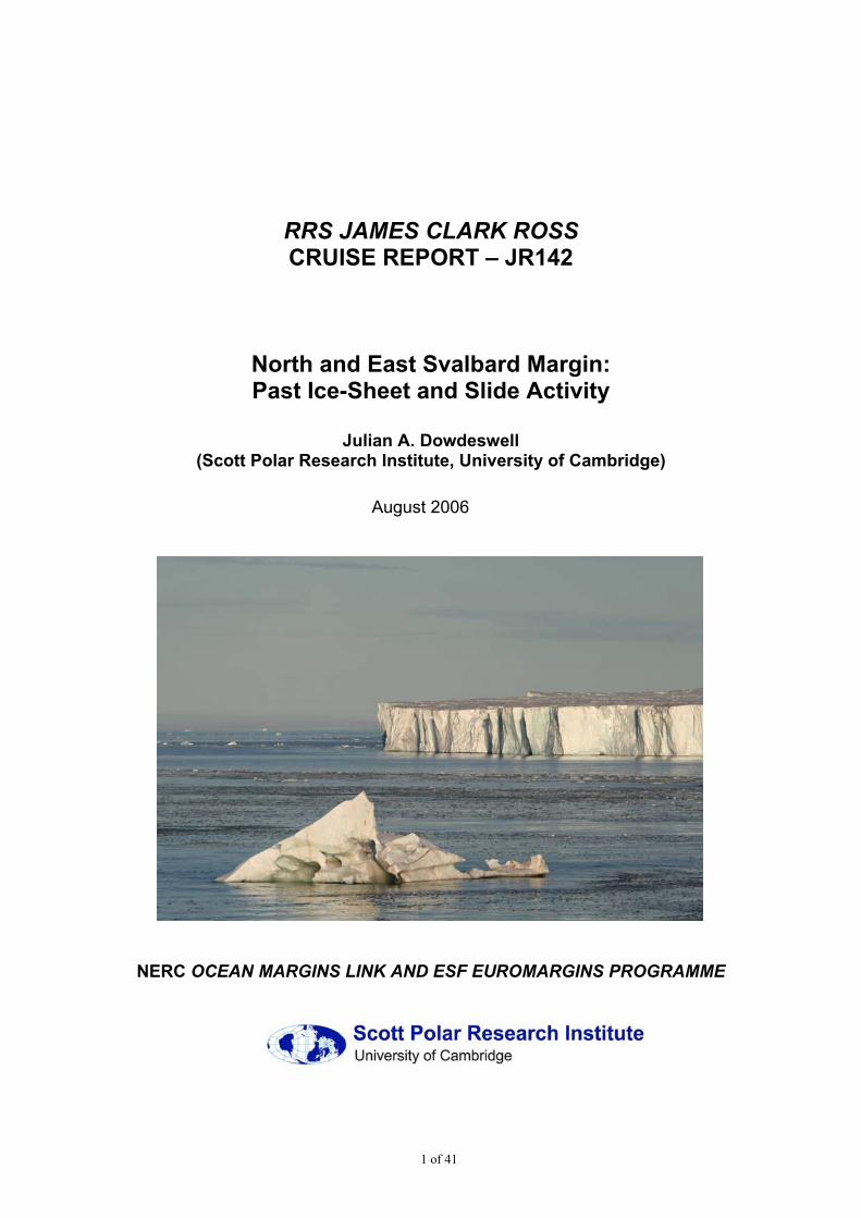
RRS JAMES CLARK ROSSCRUISE REPORT – JR142

North and East Svalbard Margin:Past Ice-Sheet and Slide Activity

Julian A. Dowdeswell(Scott Polar Research Institute, University of Cambridge)

August 2006

NERC OCEAN MARGINS LINK AND ESF EUROMARGINS PROGRAMME

2 of 41

CONTENTS

1. CRUISE JR142 NORTH AND EAST SVALBARD MARGIN1.1 Introduction: Aims and Achievements1.2 Cruise Participants1.3 Cruise Narrative

2. GEOPHYSICAL OPERATIONS – SWATH AND TOPAS2.1 EM120 Multibeam Swath Bathymetry System2.2 TOPAS Sub-Bottom Profiler2.3 EPC Chart Recorder2.4 Expendable Bathytherograph (XBT) System2.5 Oceanlogger

3. GEOPHYSICAL OPERATIONS – TOBI SIDE-SCAN SONAR3.1 System Description3.2 TOBI Deployments and Watch Keeping3.3 Instrument Performance3.4 Deliverable Items

4. GEOLOGICAL OPERATIONS4.1 Deployment and Operation of Gravity Corer4.2 Cores Acquired

5. SOME PRELIMINARY DATA: PAST ICE-SHEET AND SLIDE ACTIVITY ON THE NORTH AND EAST SVALBARD MARGIN

6. TESTS ON BACKSCATTER VALUES DERIVED FROM THE EM120

7. APPENDICES7.1 Sonar System Parameter Settings7.2 TOBI: Brief Technical Specification

3 of 41

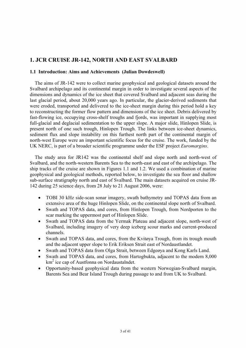
1. JCR CRUISE JR-142, NORTH AND EAST SVALBARD

1.1 Introduction: Aims and Achievements (Julian Dowdeswell)

The aims of JR-142 were to collect marine geophysical and geological datasets around theSvalbard archipelago and its continental margin in order to investigate several aspects of thedimensions and dynamics of the ice sheet that covered Svalbard and adjacent seas during thelast glacial period, about 20,000 years ago. In particular, the glacier-derived sediments thatwere eroded, transported and delivered to the ice-sheet margin during this period hold a keyto reconstructing the former flow pattern and dimensions of the ice sheet. Debris delivered byfast-flowing ice, occupying cross-shelf troughs and fjords, was important in supplying mostfull-glacial and deglacial sedimentation to the upper slope. A major slide, Hinlopen Slide, ispresent north of one such trough, Hinlopen Trough. The links between ice-sheet dynamics,sediment flux and slope instability on this furthest north part of the continental margin ofnorth-west Europe were an important scientific focus for the cruise. The work, funded by theUK NERC, is part of a broader scientific programme under the ESF project Euromargins.

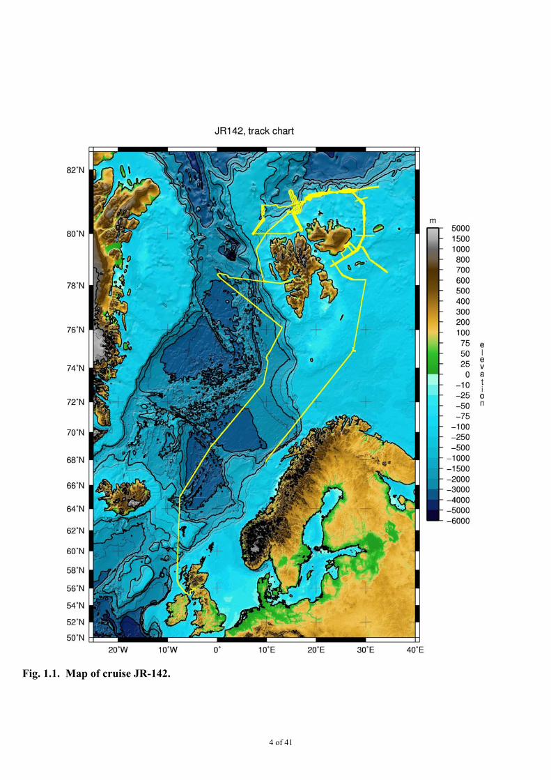
The study area for JR142 was the continental shelf and slope north and north-west ofSvalbard, and the north-western Barents Sea to the north-east and east of the archipelago. Theship tracks of the cruise are shown in Figures 1.1 and 1.2. We used a combination of marinegeophysical and geological methods, reported below, to investigate the sea floor and shallowsub-surface stratigraphy north and east of Svalbard. The main datasets acquired on cruise JR-142 during 25 science days, from 28 July to 21 August 2006, were:

• TOBI 30 kHz side-scan sonar imagery, swath bathymetry and TOPAS data from anextensive area of the huge Hinlopen Slide, on the continental slope north of Svalbard.

• Swath and TOPAS data, and cores, from Hinlopen Trough, from Nordporten to thescar marking the uppermost part of Hinlopen Slide.

• Swath and TOPAS data from the Yermak Plateau and adjacent slope, north-west ofSvalbard, including imagery of very deep iceberg scour marks and current-producedchannels.

• Swath and TOPAS data, and cores, from the Kvitøya Trough, from its trough mouthand the adjacent upper slope to Erik Eriksen Strait east of Nordaustlandet.

• Swath and TOPAS data from Olga Strait, between Edgeøya and Kong Karls Land.• Swath and TOPAS data, and cores, from Hartogbukta, adjacent to the modern 8,000

km2 ice cap of Austfonna on Nordaustalndet.• Opportunity-based geophysical data from the western Norwegian-Svalbard margin,

Barents Sea and Bear Island Trough during passage to and from UK to Svalbard.

4 of 41

Fig. 1.1. Map of cruise JR-142.

5 of 41

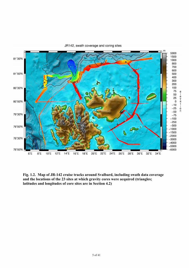
Fig. 1.2. Map of JR-142 cruise tracks around Svalbard, including swath data coverageand the locations of the 23 sites at which gravity cores were acquired (triangles;latitudes and longitudes of core sites are in Section 4.2)

6 of 41

1.2 CRUISE PARTICIPANTS

Officers and CrewGraham Chapman MasterRobert Paterson Chief OfficerCalum Hunter 2nd OfficerDouglas Leask 3rd OfficerChris Handy 3rd OfficerJohn Summers Deck OfficerCharles Waddicor ETO (Comms)David Cutting Chief EngineerGerry Armour 2nd EngineerTom Elliott 3rd EngineerSteve Eadie 4th EngineerSimon Wright Deck EngineerNicholas Dunbar ETO (ENG)Hamish Gibson PurserGeorge Stewart BosunMarc Blaby Bosun’s MateDerek Jenkins SG1Lester Jolly SG1Christopher Solly SGIJohn MacLeod SG1Cliff Mullaney SG1Mark Robinshaw MG1Sidney Smith MG1Duncan MacIntyre Chief CookGlen Ballard 2nd CookCliff Pratley Senior StewardJimmy Newall StewardKenneth Weston StewardDerek Lee Steward

ScientistsJulian Dowdeswell (PSO) SPRIJeff Evans SPRIKelly Hogan SPRIRuth Mugford SPRIRiko Noormets SPRIColm Ó Cofaigh DurhamLee Fowler TOBI Team, UKORSDuncan Matthew TOBI Team, UKORSDavid Turner TOBI Team, UKORSMark Preston BASDoug Willis BAS

SPRI Scott Polar Research Institute, University of CambridgeDurham Department of Geography, Durham UniversityUKORS, NOC TOBI Team, National Oceanography Centre, Southampton

7 of 41

1.3 CRUISE NARRATIVE (Julian Dowdeswell)

Friday 28 July, day 1JCR arrived in Longyearbyen, Svalbard, at 10.00, mooring at the coaling terminal. Thescientific party for JR142 boarded the ship and began mobilisation of TOBI and otherequipment. The ship left Longyearbyen at 15.15, sailing west along Isfjorden and thennorthward in light airs. Mountains of Prins Karls Foreland visible in the distance undercanopy of clouds.Noon position: 78 14.6 N 015 32.6 E (alongside Coal Pier in Longyearbyen, Svalbard)

Saturday 29 July, day 2Sailing northward to area of Hinlopen Slide, encountering ice over the study site. Calm andfoggy. Proceeded eastward to 81º’30N, 32º30’ENoon position: 80 24.5 N 012 26.1 E

Sunday 30 July, day 3Part of day in ice. Calm and foggy. Polar bear sighted at dinner time. Swam away leavingdead seal. Approached area of Hinlopen Slide again but ice still over it, precluding TOBIoperations in this area at present.Noon position: 81 26.4 N 028 18.3 E

Monday 31 July, day 4Fog and calm all day. Encountered band of ice in morning and saw one polar bear to port.Turned south towards the strait between Nordaustlandet and Kvitøya in afternoon. No ice inthe Kvitøya trough.Noon position: 81 21.2 N 22 43.3 E

Tuesday 1 August, day 5Sailing southwards towards Erik Eriksen Strait, with no sea ice present. Fog meant we did notsee either Austfonna or Kvitøya as we passed south between them in morning. Completedfirst southward track of about 20 hours, and turned north in Erk Eriksen Strait shortly aftermidday. Parts of Austfonna and Kong Karls Land visible in afternoon, together with about sixicebergs calved from its seaward margin. Light wind from north in evening dispersing fog.Noon position: 78 49.2 N 023 15.1 E

Wednesday 2 August, day 6Passed between Storøya and Kvitøya about 00.00. Melt features on Kvitøyjokulen clearlyvisible. Headed north to 81 in winds rising to Force 4 with slight swell. Turned southwardagain about 11.00 and in early pm saw two polar bears far from land. One was swimming, theother appeared to be floating inert. Good view of Storøya and its ice cap, with Austfonnabehind in afternoon and of Kong Karls Land and Barentsøya in evening. Several icebergssighted, including some with dirt bands.Noon position: 80 54.2 N 029 34.8 E

8 of 41

Thursday 3 August, day 7Arrived at Isispynten on east coast of Nordaustlandet am. Commenced a swath and TOBIsurvey of area from Isispynten to Hartogbukta, looking at recent deposits revealed by retreatof the ice cliffs of Austfonna and possible surging. TOBI in water from 18.00 to 21.00, towedat about 20 m depth with useful side-scan data acquired. Calm and sunny setting lookingtowards ice cliffs and interior of Austfonna. A walrus sighted pm.Noon position: 79 38.5 N 027 00.1 E

Friday 4 August, day 8Swath and TOPAS in Hartogbukta, and three cores. Closest approach to ice cliffs about 600m. Cliffs 10-20 m high in general. Weather calm and clear am, clouding over but remainingcalm pm.Noon position: 79 35.2 N 026 04.3 E

Saturday 5 August, day 9Left Hartogbukta about 02.00 for the main SW to NE swath line in Erik Eriksen Strait.Excellent views of Barentsøya, Kapp Payer and Kong Karls Land during day, with Edgeøyaand Wilhelmøya in the distance. Swath and coring during the day, with four gravity coresobtained.Noon position: 78 54.0 N 023 58.5 E

Sunday 6 August, day 10Swath in Hartogbukta overnight, then to Erik Eriksen Strait and a line of swath, TOPAS andcores taken to the north. Passed 15 nm west of Andree’s last camp on the western tip ofKvitøya pm, then to trough mouth by late evening. Weather light winds and high pressurewith cloud pm.Noon position: 79 37.8 N 028 58.1 E

Monday 7 August, day 11Swath and coring overnight. Clear morning with wind force 3. Passed tabular iceberg,probably derived from Franz Josef Land, where floating ice margins make the release of suchbergs possible. TOBI launched at 16.30 in force 4 conditions, to begin survey of HinlopenSlide. This will take about 5-6 days, depending on weather and sea-ice conditions.Noon position: 81 15.7 N 020 17.2 E

Tuesday 8 August, day 12TOBI survey continues, working east to west across Hinlopen Slide. Wind rising to force 5during day then falling slowly, with snow showers.Noon position: 81 00.0 N 016 09.6 E

Wednesday 9 August, day 13TOBI survey continues, working north to the northernmost limit of the survey on HinlopenSlide. Band of ice encountered in late afternoon meant that the final 4 km of the northernmostleg could not be completed. Saw tabular iceberg in the pack. Winds light throughout the daywith sun and snow showers.Noon position: 81 06.2 N 015 46.0 E

9 of 41

Thursday 10 August, day 14TOBI survey of Hinlopen Slide continues in fine weather with calm or very light winds.Clear views of northern Nordaustlandet, Phippsøya and Asgaardfonna in NE Spitsbergen.Saw whales pm.Noon position: 80 50.3 N 015 38.2 E

Friday 11 August, day 15Half way point in cruise. TOBI survey of Hinlopen Slide continues in fine weather. Windforce 2-4 during day.Noon position: 80 50.8 N 015 19.7 E

Saturday 12 August, day 16TOBI survey of Hinlopen Slide completed at 21.00 after encountering ice at north end ofsurvey area earlier in the day. Recovery completed in force 6 winds gusting to force 7. Beganswath work in Hinlopen Trough, in clearing weather with excellent views to northernNordaustlandet and the north coast of Spitsbergen.Noon position: 81 08.3 N 016 00.9 E

Sunday 13 August, day 17Swath work and coring in Hinlopen Trough. Four cores taken and several lines of swath data.Winds force 3 to force 6, with more shelter close to Nordporten, the northern entrance toHinlopen Strait.Noon position: 80 23.5 N 016 26.2 E

Monday 14 August, day 18Completed survey of Hinlopen Trough overnight. Passed walrus colony on island of Moffenam on passage to Yermak Plateau. Swath lines over area of deep iceberg scours on YermakPlateau for rest of the day in light winds.Noon position: 79 59.9 N 010 57.1 E

Tuesday 15 August, day 19Yermak Plateau survey area completed overnight. Interesting current-related channels seen indeeps as well as large iceberg scours. Passage then to east, with ice causing several deviationsto the south. Swath survey of scour marks east of TOBI area in rising winds from the NW,bring ice down into the survey area.Noon position: 80 56.4 N 14 49.9 E

Wednesday 16 August, day 20Moving along northern Svalbard shelf edge, but NW winds blowing sea ice into the surveyarea. Several deviations from course due to ice. Winds force 5-6. Eventually decide to headsouthwards due to adverse ice conditions.Noon position: 81 09.5 N 028 39.5 E

Thursday 17 August, day 21Overnight swath survey of area between Storøya and Kvitøya shows clear lineations in seafloor and will help define width of former ice stream. During day acquired further swath andTOPAS data from Hartogbukta in calm to light winds.

10 of 41

Noon position: 79 38.2 N 026 39.1 E

Friday 18 August, day 22Overnight began eastward swath and TOPAS survey across Erk Erikson Strait and passedAbeløya, the most easterly island of Kong Karls Land. Working across trough that leads toFranz Victoria Trough in the Russian zone in light winds with slight swell. Turned north-westagain at our furthest east, 34 30’E.Noon position: 78 37.0 N 033 44.2 E

Saturday 19 August, day 23Continued swath mapping area east of Kong Karls Land and took two cores in the morning.Then returned SW down Erik Eriksen Strait in light winds but overcast conditions inafternoon. Among icebergs calved from Bråsvellbreen in evening, with good view of this icefront and Sorporten, the southern entrance to Hinlopen Strait.Noon position: 79 22.5 N 029 46.0 E

Sunday 20 August, day 24Swath mapping and TOPAS in Olga Strait, between Edgeøya and Kong Karls Landthroughout the day with light winds and overcast skies.Noon position: 78 24.5 N 025 31.0 E

Monday 21 August, day 25Completed survey of Olga Strait by about 04.00 and proceeded south into the Barents Seawith the end of the scientific activity on the cruise. Final short swath survey of fluted seafloor on north side of Bear Island Trough in evening.Noon position: 76 55.8 N 28 55.7 E

Tuesday 22 August, day 26Crossing Bear Island Trough on passage to UK. Weather foggy by very light winds.Noon position: 73 21.1 N 22 53.2 E

Wednesday 23 August, day 27On passage to UK, passing Lofoten Islands, north Norway. Winds up to force 4-5 inafternoon.Noon position: 69 31.2 N 13 19.2 E

Thursday 24 August, day 28On passage to UK, passing Trondheim and oil platforms of Asgard field en route. Weatherfine and winds light.Noon position: 65 04.3 N 05 51.8 E

Friday 25 August, day 29On passage to UK, in North Sea. Cruise dinner in evening after drinks on deck.Noon position: 60 21.1 N 03 12.4 E

Saturday 26 August, day 30On passage to UK, in North Sea. Calm conditions.

11 of 41

Noon position: 55 52.9 N 01 14.8 E

Sunday 27 August, day 31Docked in Immingham, UK, after passing through the locks on the morning tide.

12 of 41

2. GEOPHYSICAL OPERATIONS – SWATH AND TOPAS (Jeffrey Evans, Kelly Hogen, Ruth Mugford, Riko Noormets and Colm Ó Cofaigh)

2.1 EM120 Multibeam Swath Bathymetry System The Kongsberg-Simrad EM120 multibeam swath bathymetry system was operatedthroughout the cruise. Angular coverage was set to “Manual” and beam spacing was set to“Equidistant”. The beam angle used varied according to sea conditions, water depth and sea-bed type but was generally between 64-68 degrees. During surveys, overlap betweenindividual swath lines was achieved by means of the Helmsman’s Display on the bridge,which the Bridge Officer used to adjust the ship’s course and maintain a reasonable degree ofoverlap (10%) between lines. Limited post-processing of the EM120 data (gridding and datafiltering) was carried out using the Kongsberg-Simrad NEPTUNE post-processing software.In general the EM120 worked well throughout the cruise, although some problems wereencountered in triggering from the SSU. Where the system lost the sea-bed from time to timethe most useful method was to use the “Force Depth” command with a depth slightly lessthan the true seabed. Restricting the maximum and minimum depths to a tight range aroundthe true seabed depth was also useful as well as reducing the angle of the beams. The EM120 system performed well most of the time with the exception being in veryshallow water when SSU triggering of the EM120 and TOPAS resulted in dropouts in swathcoverage. The ITS and ETS worked to solve this problem during the cruise and this is stillon-going. This problem was worked around by manual triggering of swath and TOPAS. Ason previous cruises where the EM120 was used in pack ice (e.g. JR84 and JR104), it wasfound that when the ship was moving through the ice the swath signal deterioratedsignificantly. Leeway when wind is on the beam is a well known cause of poor quality inswath data and this occurred on few occasions. Due to the generally light winds on the cruise,this was a problem on only a very few occasions. However, the signal returns in only a fewmetres of open water. The EM120 acquisition parameters used are described in Appendix 7.1.

2.2. TOPAS Sub-Bottom Profiler The TOPAS system was used extensively throughout the cruise and generally performedvery well. As in the case of the EM120, sea ice affects the TOPAS signal quite badly. Itresults in many high amplitude signals resulting in dark traces across the record. In heavy seaice this can have the result of obliterating any meaningful data. In water depths of less than1000 m we ran TOPAS using a Burst mode whereas in depths greater than this we used theChirp (see Appendix 1 for TOPAS acquisition parameters).

2.3 EPC Chart Recorder The EPC chart recorder worked without any problems throughout the cruise. TOPAS inputto the EPC chart recorder was on Channel A. The settings used were: 0.5 second sweep; 0delay; threshold 1/3 of a turn clockwise from the minimum setting; trigger level 0; gaingenerally about 8; sweep direction from left to right; print polarity +/- (centre setting). Chartsettings: scale lines: on; take-up: on; mark/annotate: off (centre setting); chart drive: internal(centre setting), LPI was generally set to 75; contrast setting: centre. Ten-minute time marksand EM120 depths were automatically plotted on the paper roll.

13 of 41

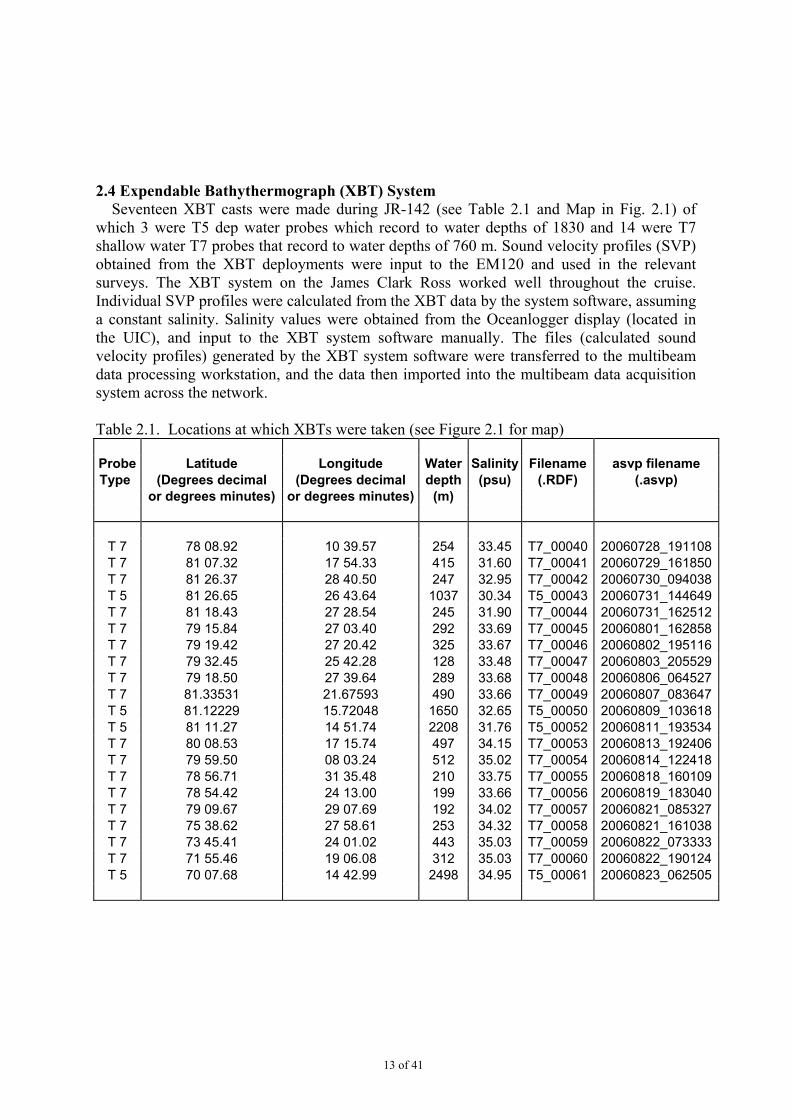
2.4 Expendable Bathythermograph (XBT) System Seventeen XBT casts were made during JR-142 (see Table 2.1 and Map in Fig. 2.1) ofwhich 3 were T5 dep water probes which record to water depths of 1830 and 14 were T7shallow water T7 probes that record to water depths of 760 m. Sound velocity profiles (SVP)obtained from the XBT deployments were input to the EM120 and used in the relevantsurveys. The XBT system on the James Clark Ross worked well throughout the cruise.Individual SVP profiles were calculated from the XBT data by the system software, assuminga constant salinity. Salinity values were obtained from the Oceanlogger display (located inthe UIC), and input to the XBT system software manually. The files (calculated soundvelocity profiles) generated by the XBT system software were transferred to the multibeamdata processing workstation, and the data then imported into the multibeam data acquisitionsystem across the network.

Table 2.1. Locations at which XBTs were taken (see Figure 2.1 for map)

Probe Latitude Longitude Water Salinity Filename asvp filename Type (Degrees decimal (Degrees decimal depth (psu) (.RDF) (.asvp)

or degrees minutes) or degrees minutes) (m)

T 7 78 08.92 10 39.57 254 33.45 T7_00040 20060728_191108T 7 81 07.32 17 54.33 415 31.60 T7_00041 20060729_161850T 7 81 26.37 28 40.50 247 32.95 T7_00042 20060730_094038T 5 81 26.65 26 43.64 1037 30.34 T5_00043 20060731_144649T 7 81 18.43 27 28.54 245 31.90 T7_00044 20060731_162512T 7 79 15.84 27 03.40 292 33.69 T7_00045 20060801_162858T 7 79 19.42 27 20.42 325 33.67 T7_00046 20060802_195116T 7 79 32.45 25 42.28 128 33.48 T7_00047 20060803_205529T 7 79 18.50 27 39.64 289 33.68 T7_00048 20060806_064527T 7 81.33531 21.67593 490 33.66 T7_00049 20060807_083647T 5 81.12229 15.72048 1650 32.65 T5_00050 20060809_103618T 5 81 11.27 14 51.74 2208 31.76 T5_00052 20060811_193534T 7 80 08.53 17 15.74 497 34.15 T7_00053 20060813_192406T 7 79 59.50 08 03.24 512 35.02 T7_00054 20060814_122418T 7 78 56.71 31 35.48 210 33.75 T7_00055 20060818_160109T 7 78 54.42 24 13.00 199 33.66 T7_00056 20060819_183040T 7 79 09.67 29 07.69 192 34.02 T7_00057 20060821_085327T 7 75 38.62 27 58.61 253 34.32 T7_00058 20060821_161038T 7 73 45.41 24 01.02 443 35.03 T7_00059 20060822_073333T 7 71 55.46 19 06.08 312 35.03 T7_00060 20060822_190124T 5 70 07.68 14 42.99 2498 34.95 T5_00061 20060823_062505

14 of 41

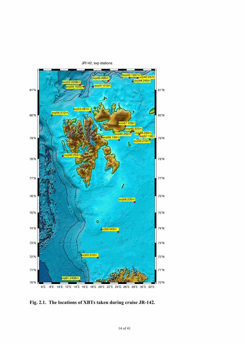
Fig. 2.1. The locations of XBTs taken during cruise JR-142.

15 of 41

2.5 Oceanlogger The Oceanlogger was operated during JR-142 in order to monitor changes in surface watercharacteristics that affect sound propagation, and to measure surface water salinity values forcalculation of SVP’s from XBT data.

16 of 41

3. GEOPHYSICAL OPERATIONS – TOBI SIDE-SCAN SONAR(TOBI Team: Duncan Matthew, Lee Fowler, David Turner)

3.1 System Description

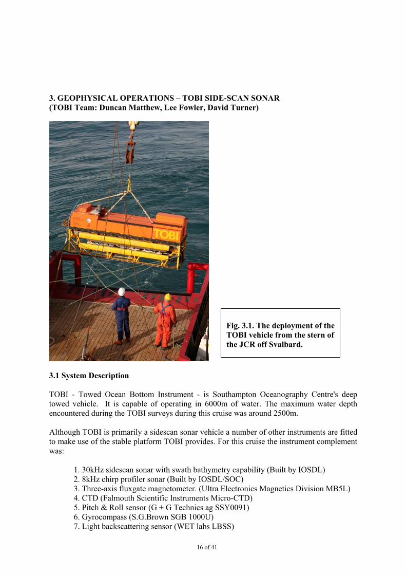
TOBI - Towed Ocean Bottom Instrument - is Southampton Oceanography Centre's deeptowed vehicle. It is capable of operating in 6000m of water. The maximum water depthencountered during the TOBI surveys during this cruise was around 2500m.

Although TOBI is primarily a sidescan sonar vehicle a number of other instruments are fittedto make use of the stable platform TOBI provides. For this cruise the instrument complementwas:

1. 30kHz sidescan sonar with swath bathymetry capability (Built by IOSDL)2. 8kHz chirp profiler sonar (Built by IOSDL/SOC)3. Three-axis fluxgate magnetometer. (Ultra Electronics Magnetics Division MB5L)4. CTD (Falmouth Scientific Instruments Micro-CTD)5. Pitch & Roll sensor (G + G Technics ag SSY0091)6. Gyrocompass (S.G.Brown SGB 1000U)7. Light backscattering sensor (WET labs LBSS)

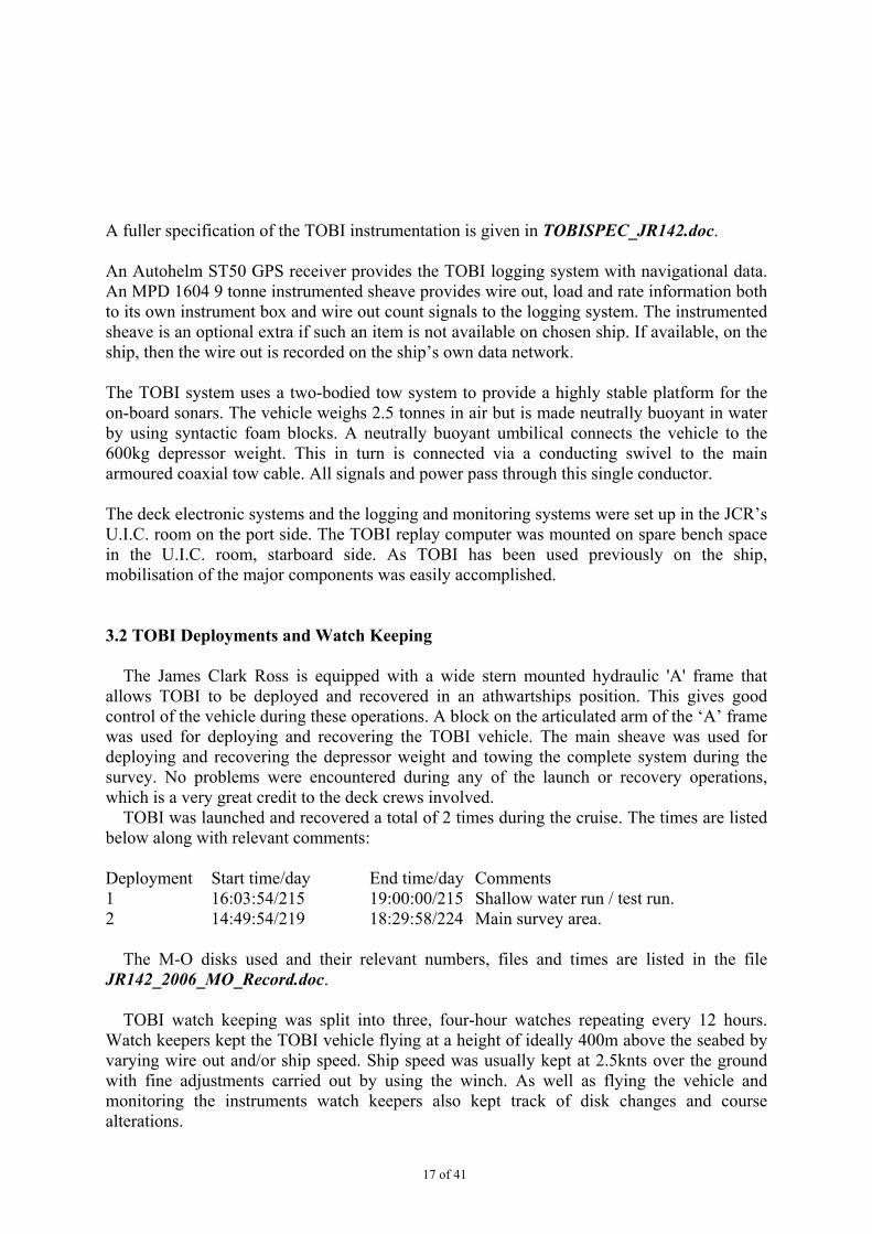
Fig. 3.1. The deployment of theTOBI vehicle from the stern ofthe JCR off Svalbard.

17 of 41

A fuller specification of the TOBI instrumentation is given in TOBISPEC_JR142.doc.

An Autohelm ST50 GPS receiver provides the TOBI logging system with navigational data.An MPD 1604 9 tonne instrumented sheave provides wire out, load and rate information bothto its own instrument box and wire out count signals to the logging system. The instrumentedsheave is an optional extra if such an item is not available on chosen ship. If available, on theship, then the wire out is recorded on the ship’s own data network.

The TOBI system uses a two-bodied tow system to provide a highly stable platform for theon-board sonars. The vehicle weighs 2.5 tonnes in air but is made neutrally buoyant in waterby using syntactic foam blocks. A neutrally buoyant umbilical connects the vehicle to the600kg depressor weight. This in turn is connected via a conducting swivel to the mainarmoured coaxial tow cable. All signals and power pass through this single conductor.

The deck electronic systems and the logging and monitoring systems were set up in the JCR’sU.I.C. room on the port side. The TOBI replay computer was mounted on spare bench spacein the U.I.C. room, starboard side. As TOBI has been used previously on the ship,mobilisation of the major components was easily accomplished.

3.2 TOBI Deployments and Watch Keeping

The James Clark Ross is equipped with a wide stern mounted hydraulic 'A' frame thatallows TOBI to be deployed and recovered in an athwartships position. This gives goodcontrol of the vehicle during these operations. A block on the articulated arm of the ‘A’ framewas used for deploying and recovering the TOBI vehicle. The main sheave was used fordeploying and recovering the depressor weight and towing the complete system during thesurvey. No problems were encountered during any of the launch or recovery operations,which is a very great credit to the deck crews involved. TOBI was launched and recovered a total of 2 times during the cruise. The times are listedbelow along with relevant comments:

Deployment Start time/day End time/day Comments1 16:03:54/215 19:00:00/215 Shallow water run / test run.2 14:49:54/219 18:29:58/224 Main survey area.

The M-O disks used and their relevant numbers, files and times are listed in the fileJR142_2006_MO_Record.doc.

TOBI watch keeping was split into three, four-hour watches repeating every 12 hours.Watch keepers kept the TOBI vehicle flying at a height of ideally 400m above the seabed byvarying wire out and/or ship speed. Ship speed was usually kept at 2.5knts over the groundwith fine adjustments carried out by using the winch. As well as flying the vehicle andmonitoring the instruments watch keepers also kept track of disk changes and coursealterations.

18 of 41

The bathymetry charts of the work area comprised of previously surveyed blocks andEM120 runs prior to deployment. Both of these helped immensely when flying the vehicle.

3.3 Instrument Performance

These are real time observations of the instrumentation performance. A more detailedengineering analysis, involving the data collected, will home in on problem areas highlightedby these observations.

Vehicle

Pre-survey tests revealed a problem with the CTD causing no and/or incorrect data strings,comprising of CTD and gyro readings, reaching the logging and digital display computers. Abench test of the CTD unit revealed that it was in an incorrect mode. The mode was changedto the required setting and the correct data stream was observed. The CTD was re-attached tothe vehicle which was then powered up and the data strings were now correct. Run 1 was short (3 hours) and the vehicle performed well for such a shallow area, 220 –240 meters water depth. Run 2 was the primary work area comprising of 5 days survey timein water depths of 100 – 2500 metres. During the 2 runs the vehicle performed well apart from a number of remote ‘reboots’ ofthe CTD/Gyro interface and occasional ‘power cycling’ of the vehicle to get the CTD/Gyrodata stream back online. Further into the run it was found that only remote ‘reboots’ of theCTD /gyro interface with adequate wait times to restart precluded any need to ‘power cycle’.This allowed the sonar data stream to continue and only the CTD/gyro data to be incorrect forsuch short (2 – 3 minute) periods. There were two (2) instances of ‘loss of trigger pulses’ towards the end of Run#2, a veryrare occurrence, which produced gaps in the data files due to corrupted files. The vastmajority of the data in the effected files were successfully recovered. The umbilical and electrical swivel performed well with no down time.

Profiler

The system preformed well although the altitude tracking had to be turned off and entered inmanually. This was due to the large number of multiple echoes inherent in shallow waterwork which confused the auto tracking algorithm.

Sidescan

The system performed well with excellent records of slopes and debris flow.

Magnetometer

The unit worked well throughout the cruise. The output did lock up (frozen display values)when a power cycle was conducted too quickly. A few minutes of power down to allowvoltages to fully fall solved this. No calibration of the magnetometer in the vehicle was

19 of 41

undertaken although there should be enough data within the survey to carry one out postcruise.

Gyro

The unit performed well with the data stream only being corrupted when the CTD locked up.The system returned to normal once the CTD had been correctly rebooted.

CTD – FSI Serial No. 1426-09nov98

For the majority of the cruise the CTD worked well once the system was set to the right modeduring the initial deck test. During the survey the unit had to be rebooted 38 times. This hadthe effect of freezing the CTD and gyrocompass readings until the CTD could be fullyrebooted. Due to time pressure and the ability to reboot the unit remotely it was decided notto recover the vehicle to try one of the other spares. A full assessment of this unit, in and outof the vehicle, will be done back at NOC.

Pitch/Roll

This unit performed well for the whole cruise.

LSS

The light scattering sensor was used throughout the cruise. Although the data was notrequired on this cruise it is available in the TOBI data files.

Swath bathymetry

The unit performed well with only occasional periods of the port side being washed out at thefar range. From observations, in this cruise, it could be seen that there is a good 1.5km rangefor the starboard swath with approximately 1km for the port side.

20 of 41

Deck Unit

The system proved very reliable in operation throughout the cruise. A voltage of 320V wasused to power the vehicle with a current of approximately 300mA.

Instrumented Sheave. Not required on this cruise, JCR had the facilities in place and wire outdata made available in a text file.

Winch – TOBI Portable. Not required on this cruise, JCR had a fully operational deep towwinch with an inner coaxial cable for power, communication and data streams.

Data Recording and Display

Data from the TOBI vehicle is recorded onto 1.2Gbyte magneto-optical (M-O) disks. Oneside of each disk gives approximately 16 hours 9 minutes of recording time. All data from thevehicle is recorded along with the ship position taken from the TOBI portable GPS receiver.Data was recorded using TOBI programme LOG. As well as recording sidescan and digital telemetry data LOG displays real-time slantrange corrected sidescan and logging system data, and outputs the sidescan to a RaytheonTDU850 thermal recorder. PROFDISP displays the chirp profiler signals and outputs them toa Raytheon TDU850. DIGIO9 displays the real-time telemetry from the vehicle –magnetometer, CTD, pitch and roll, LSS – plus derived data such as sound speed, heading,depth, vertical rate and salinity. LOG, PROFDISP and DIGIO9 are all run on separate computers, each having its owndedicated interface systems. Data recorded on the M-O disks were copied onto CD-ROMs for archive and forimportation into the portable (NOC), available on board, image processing system (PRISM). On M-O disk 961 – TOBI.DAT the wrong date was recorded. This was corrected on a turnand from disk 961 – TOBIA.DAT onwards the date is correct. It was noted that RUN#1, fourdays prior, had the correct day. M-O disk 967 suffered from corrupted files during a period of two (2) losses of the main 4second system trigger pulses. The files were recovered but with a loss of 54 minutes and 10seconds of data. This loss was during a long 180 degree turn and zigzag route, to avoid icesheets, which took the vehicle track within a previously covered line. The loss of data istherefore reduced in importance. The Logging PC will be investigated back at base for any reoccurrence of this anomaly.

3.4 Deliverable Items• Copies of M-O data discs on CD-ROM plus associated document files, numbered 960

– 968.• Real Time thermal printout of raw sidescan (only Time Varied Gain T.V.G. applied).• Real Time thermal printout of raw non-motion compensated profiler (made available

but not generally looked at).• Replayed thermal printout of motion compensated profiler data.

21 of 41

Summary

The system performed well, overall, with some excellent sidescan imagery. The system willbe reviewed, in light of the reported faults, back at NOC in preparedness for next year’scruise program. The most likely candidate is the CTD unit as most of the reboots and powercycling revolved around getting it restarted.

Reference and ContactsTOBI technical reference: ‘TOBI, a vehicle for deep ocean survey’, C. Flewellen, N. Millardand I. Rouse, Electronics and Communication Engineering Journal April 1993.e-mail: dlrm@noc.soton.ac.ukurl: http://www.noc.soton.ac.uk

M-ONumber

File Name Time/ DaySTART

Time/ DaySTOP

Comments/ Run #

RawS/Sca

nRoll #

Corrected

ProfilerRoll #

960 TOBI.DAT 16:03:54 / 215 19:00:00 / 215 Run #1 1 1

961TOBI.DAT

TOBIA.DAT

14:49:54 /216(219)

23:32:08 / 219

23:29:06 /216(219)

07:01:46 / 220

Run #2

Loggingstopped ona 180 deg.turn to resetdate 216->219Vehicle onturnbetweenWP1 ->WP2

2 2

962TOBI.DAT

TOBIA.DAT

TOBIB.DAT

07:01:50 / 220

19:08:44 / 220

21:36:36 / 220

19:05:52 / 220

21:35:16 / 220

22:34:24 / 220

Run#2

Powerrecycle

Powerrecycle

Powerrecycle

2 3

963TOBI.DAT

TOBIA.DAT

22:50:50 / 220

08:46:24 / 221

08:42:56 / 221

11:07:26 / 221

Run#2

Powerrecycle

2 4

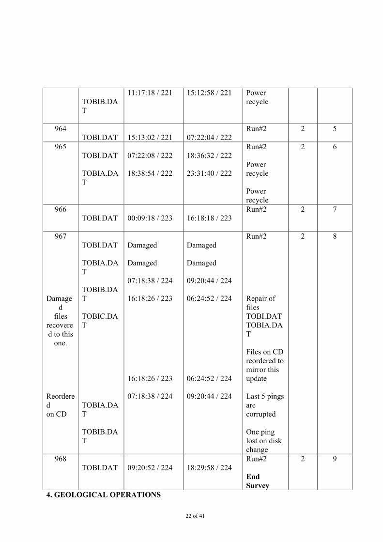
22 of 41

TOBIB.DAT

11:17:18 / 221 15:12:58 / 221 Powerrecycle

964TOBI.DAT 15:13:02 / 221 07:22:04 / 222

Run#2 2 5

965TOBI.DAT

TOBIA.DAT

07:22:08 / 222

18:38:54 / 222

18:36:32 / 222

23:31:40 / 222

Run#2

Powerrecycle

Powerrecycle

2 6

966TOBI.DAT 00:09:18 / 223 16:18:18 / 223

Run#2 2 7

967

Damaged

filesrecovered to this

one.

Reorderedon CD

TOBI.DAT

TOBIA.DAT

TOBIB.DAT

TOBIC.DAT

TOBIA.DAT

TOBIB.DAT

Damaged

Damaged

07:18:38 / 224

16:18:26 / 223

16:18:26 / 223

07:18:38 / 224

Damaged

Damaged

09:20:44 / 224

06:24:52 / 224

06:24:52 / 224

09:20:44 / 224

Run#2

Repair offilesTOBI.DATTOBIA.DAT

Files on CDreordered tomirror thisupdate

Last 5 pingsarecorrupted

One pinglost on diskchange

2 8

968TOBI.DAT 09:20:52 / 224 18:29:58 / 224

Run#2

EndSurvey

2 9

4. GEOLOGICAL OPERATIONS

23 of 41

4.1 Deployment and Operation of Gravity Corer(Dave Turner, Lee Fowler, Duncan Matthew)

NMFD Personnel: Dave Turner, Duncan Matthew, Lee FowlerNo. Cores Taken: 23

Seabed Coring System – Gravity Core

The Gravity Core System consists of a 1000kg bomb (weight), 3m core barrels with liners, acore catcher and cutter. The 3m core barrels can be joined together to give a 6m coringsystem. The deployment system consists of a coring bucket, davit and the use of the shipsStbd ‘A’ frame, coring winch and warp. The warp is secured to the core bomb using a 5tswivel. The core bucket, complete with the core bomb and barrel(s) is moved from the inboardposition to the deployment position over the side of the ship, using the core bucket hydraulicram and system davit. From this position the locking gate on the bucket is released and thesystem is rotated from the horizontal to the vertical using the davit. In the vertical positionthe core bucket is secured by the gate locking mechanism, and the bomb to bucket retainingchain is removed. The ship’s ‘A’ frame and winch lift the core bomb and barrel(s) from thebucket and the system is lowered into the water. At approximately 50 meters from reaching the seabed the winch is stopped to allow thecorer to settle in the water column for a few minutes. The winch then proceeds at a speed ofapproximately 60m/min until the corer hits the seabed. This is indicated with the load on thewire significantly dropping off, or visually, with the sheave block ‘kicking’ back. The corewire is then paid out a further 10 to 15 meters. The winch then starts to haul at approximately10m/min until the corer has left the bottom, this is indicated by a slight ‘pullout’ tension onthe cable monitoring system, or again visually, by the sheave block. Once off the bottom thesystem is brought to the surface for recovery. Haul and veer speeds through the watercolumn will be determined by the capabilities of the ships winch system, but generallyaround 60m/min. Recovery is the reverse of the deployment.

System Performance:

The coring system worked well for the majority of the cruise with one minor incidentreported (See attached near miss report). The minor equipment failure meant that the shipsmid-ships crane had to be deployed to aid the recovery of the coring system, which in turntook a little longer to get the corer secured ready for sampling. This procedure did not affectthe coring sample or generate a significant amount of science down time. Equipment repairswere carried out with no complications, or loss of time to the science program.

Near Miss Report JR142

24 of 41

National Marine Facilities Division (NMFD) Gravity Core System.

Date & Time: 17-08-06, 14:17 hrs GMTPosition: Lat 79.593166N, Lon 26.192966EWeather conditions: Sea State 1-2

Wind Speed approx 12-14 kntsShips location of incident: Stbd SideNMFD operators at time of incident: Dave Turner and Lee Fowler

Description of the event:

The Core bomb (weight) and barrel had been recovered into the core bomb cradle, and secured withits chain over the top. The Core bomb and barrel were then rotated from the vertical position to thehorizontal, using the system davit. The core bomb bucket was then secured horizontally using thelocking gate mechanism. The bucket, complete with the bomb and the barrel then proceeded to move inboard using the bombbucket hydraulic ram and system davit. This process was stopped prior to reaching the inboardposition, realizing that the core barrel had not been washed down yet. The hydraulic ram and system davit was then reversed, as with any deployment, to move the bombbucket and barrel outboard again. As the hydraulic ram reached the outer end of its stroke, the fixings on the inboard end of the ramgave way, releasing the ram and allowing the bomb bucket to swing over the side. The bucket wassecured from swinging any further by its own pivot points. To recover the situation the mid-ships crane was deployed and a strop secured to the bomb bucket.The bucket, complete with the core bomb and barrel was then lifted, slewed inboard, and secured intoits inboard position. The two bolts used for the transportation and lifting of the bucket were then putinto place locking the system inboard in the absence of the hydraulic ram. The removal of the barreland core sample was then carried out in the usual manner. On the inspection of the failure afterwards, it was found that the inboard fixing studs (4 off), to thehydraulic ram had failed due hidden excessive corrosion on the under side of the hydraulic rammounting point. The securing studs had originally been welded to the under side of the fixing plate,but due to the corrosion had pulled out when the hydraulic ram had extended. To return the coring system to an operational status the stud holes were cleaned out, and thehydraulic ram secured to the plate using 4 off M12 x 40 st/st bolts. The system was then fully tested for operational use.

25 of 41

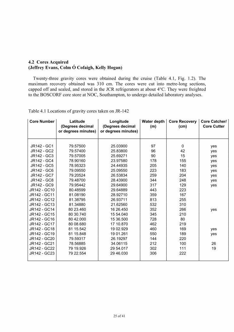
4.2 Cores Acquired(Jeffrey Evans, Colm Ó Cofaigh, Kelly Hogan)

Twenty-three gravity cores were obtained during the cruise (Table 4.1, Fig. 1.2). Themaximum recovery obtained was 310 cm. The cores were cut into metre-long sections,capped off and sealed, and stored in the JCR refrigerators at about 4°C. They were freightedto the BOSCORF core store at NOC, Southampton, to undergo detailed laboratory analyses.

Table 4.1 Locations of gravity cores taken on JR-142

Core Number Latitude Longitude Water depth Core Recovery Core Catcher/(Degrees decimal (Degrees decimal (m) (cm) Core Cutter

or degrees minutes) or degrees minutes)

JR142 - GC1 79.57500 25.03900 97 0 yesJR142 - GC2 79.57400 25.83800 96 42 yesJR142 - GC3 79.57005 25.69271 90 15 yesJR142 - GC4 78.90160 23.97580 178 155 yesJR142 - GC5 78.95323 24.44935 205 140 yesJR142 - GC6 79.09550 25.09550 223 183 yesJR142 - GC7 79.20524 26.53834 259 204 yesJR142 - GC8 79.48700 28.43900 344 248 yesJR142 - GC9 79.95442 29.64900 317 129 yes

JR142 - GC10 80.48599 29.64889 443 223JR142 - GC11 81.08190 28.92710 359 167JR142 - GC12 81.38795 26.93711 813 255JR142 - GC13 81.34880 21.62560 532 310JR142 - GC14 80 23.460 16 26.450 352 266 yesJR142 - GC15 80 30.740 15 54.040 345 210JR142 - GC16 80 42.000 15 36.500 728 80JR142 - GC17 80 08.680 17 10.870 462 219JR142 - GC18 81 15.542 19 02.929 460 169 yesJR142 - GC19 81 15.848 19 01.261 550 189 yesJR142 - GC20 79.59317 26.19297 144 220JR142 - GC21 78.56885 34.06115 212 100 26JR142 - GC22 79 19.926 29 54.017 302 111 19JR142 - GC23 79 22.554 29 46.030 306 222

26 of 41

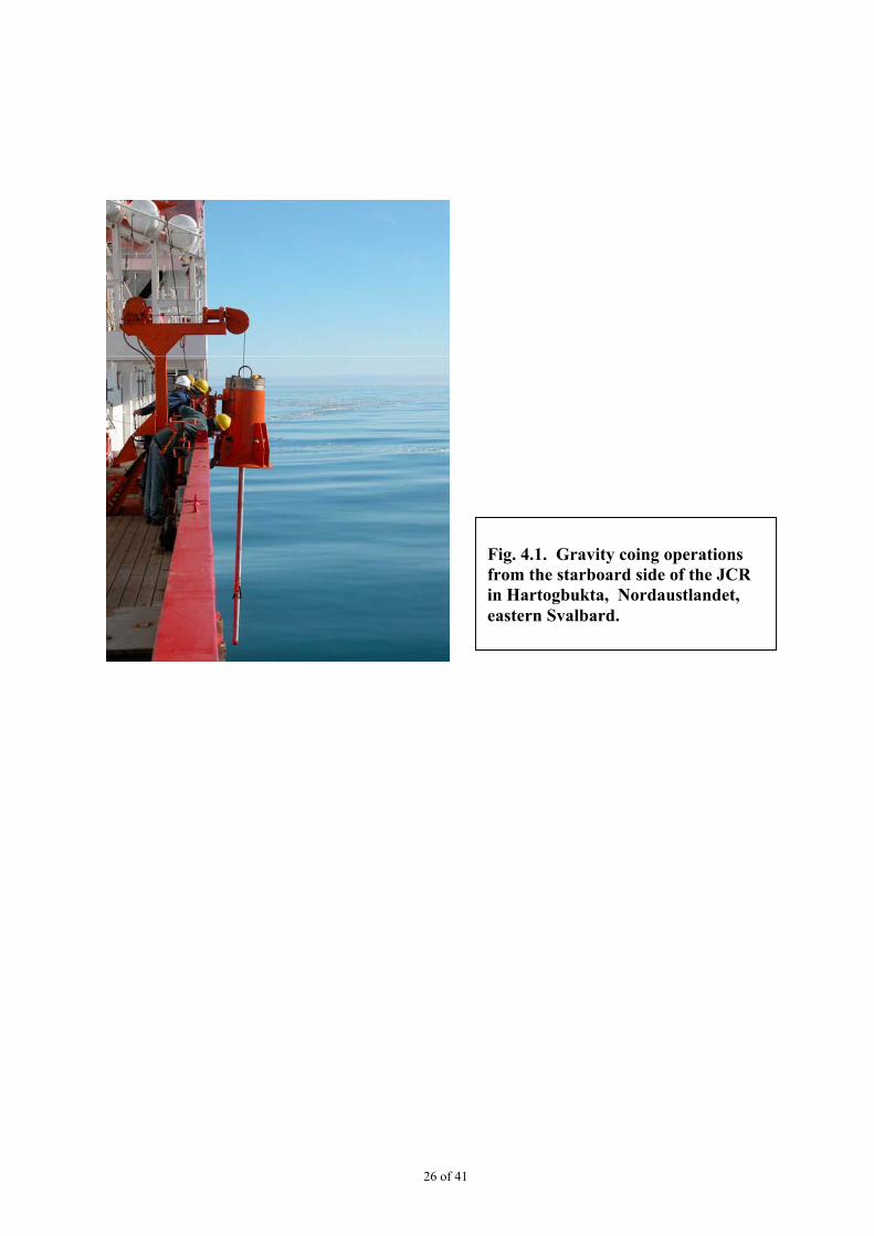
Fig. 4.1. Gravity coing operationsfrom the starboard side of the JCRin Hartogbukta, Nordaustlandet,eastern Svalbard.

27 of 41

5. SOME PRELIMINARY DATA: PAST ICE-SHEET AND SLIDE ACTIVITY ON THE NORTH AND EAST SVALBARD MARGIN

(J.A. Dowdeswell, J. Evans, K. Hogan, R. Mugford, R. Noormets, C. Ó Cofaigh)

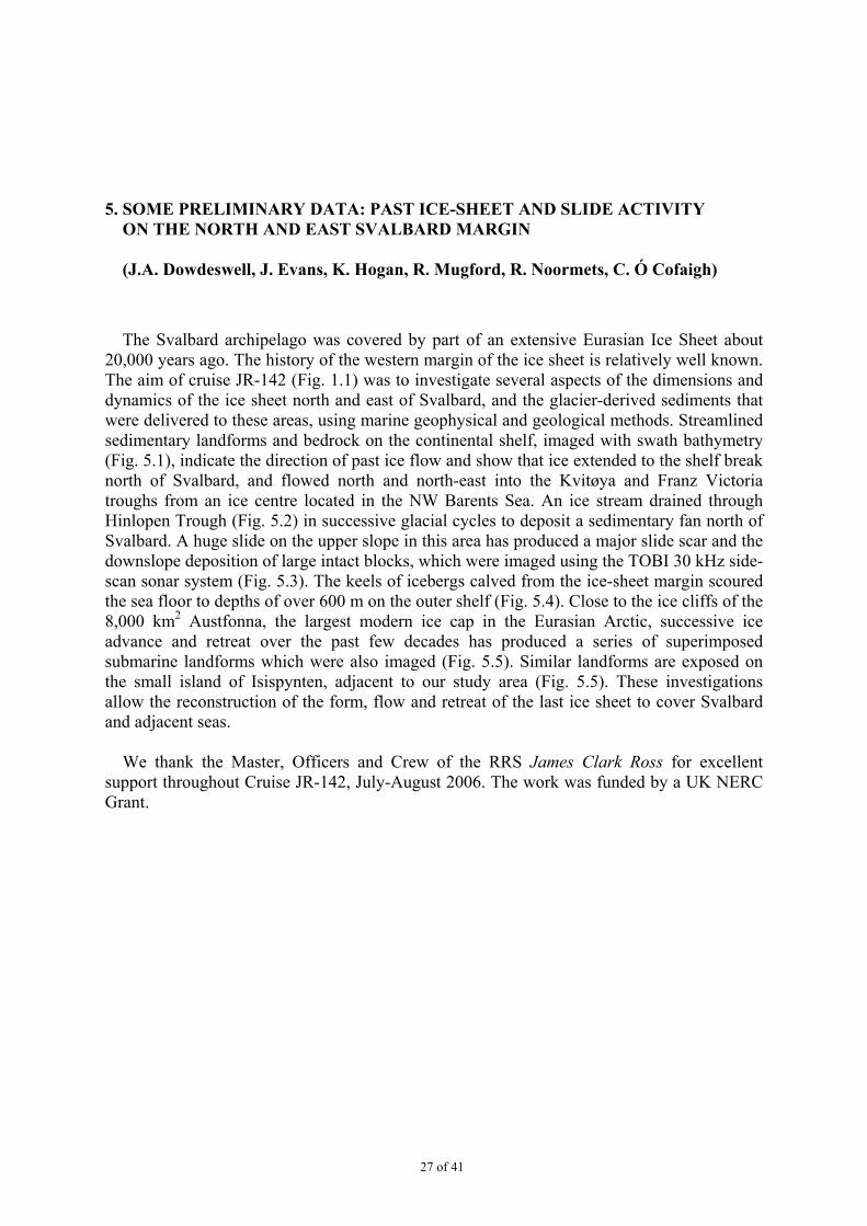
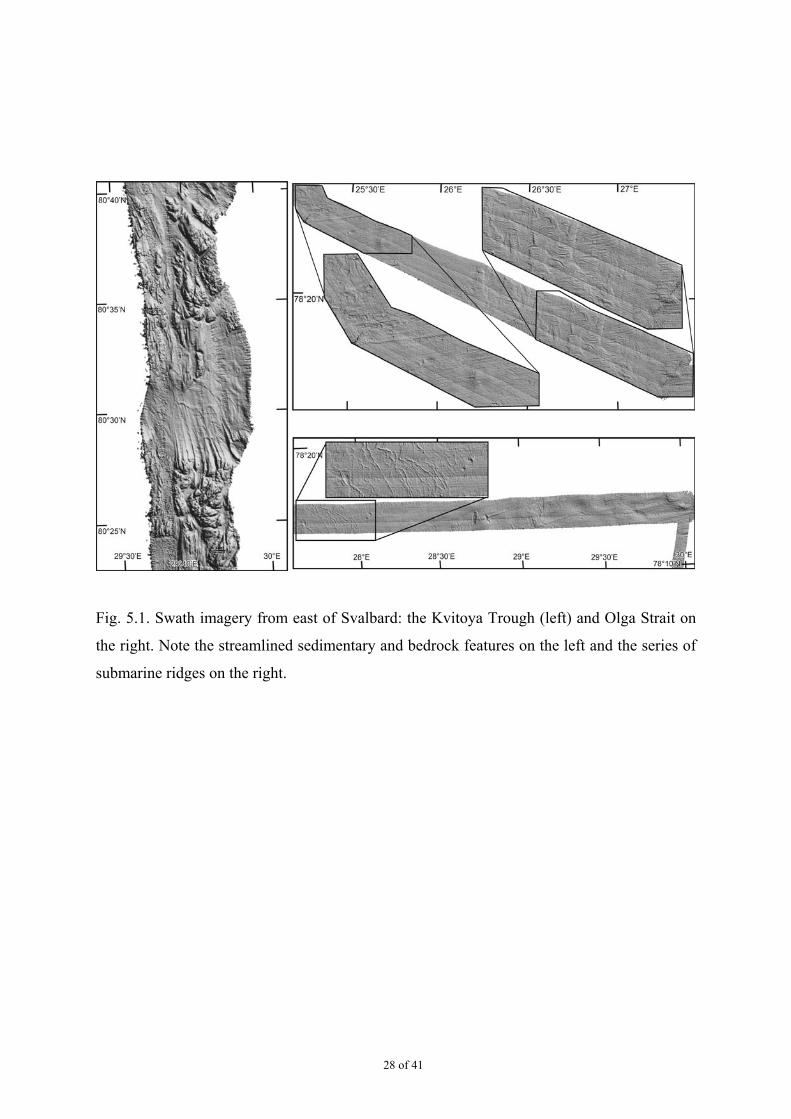
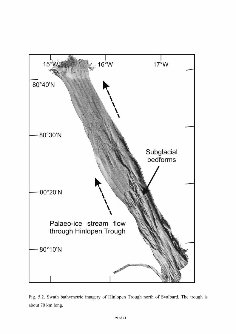
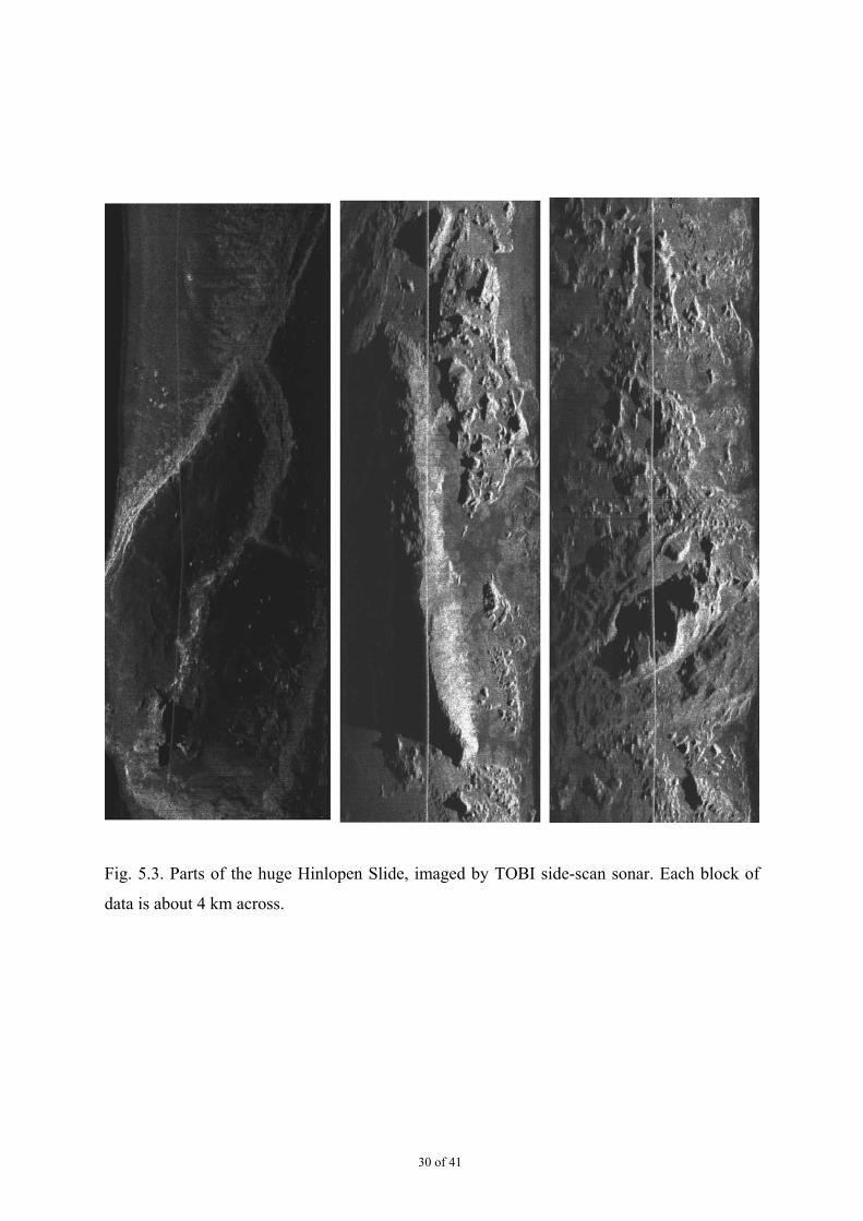
The Svalbard archipelago was covered by part of an extensive Eurasian Ice Sheet about20,000 years ago. The history of the western margin of the ice sheet is relatively well known.The aim of cruise JR-142 (Fig. 1.1) was to investigate several aspects of the dimensions anddynamics of the ice sheet north and east of Svalbard, and the glacier-derived sediments thatwere delivered to these areas, using marine geophysical and geological methods. Streamlinedsedimentary landforms and bedrock on the continental shelf, imaged with swath bathymetry(Fig. 5.1), indicate the direction of past ice flow and show that ice extended to the shelf breaknorth of Svalbard, and flowed north and north-east into the Kvitøya and Franz Victoriatroughs from an ice centre located in the NW Barents Sea. An ice stream drained throughHinlopen Trough (Fig. 5.2) in successive glacial cycles to deposit a sedimentary fan north ofSvalbard. A huge slide on the upper slope in this area has produced a major slide scar and thedownslope deposition of large intact blocks, which were imaged using the TOBI 30 kHz side-scan sonar system (Fig. 5.3). The keels of icebergs calved from the ice-sheet margin scouredthe sea floor to depths of over 600 m on the outer shelf (Fig. 5.4). Close to the ice cliffs of the8,000 km2 Austfonna, the largest modern ice cap in the Eurasian Arctic, successive iceadvance and retreat over the past few decades has produced a series of superimposedsubmarine landforms which were also imaged (Fig. 5.5). Similar landforms are exposed onthe small island of Isispynten, adjacent to our study area (Fig. 5.5). These investigationsallow the reconstruction of the form, flow and retreat of the last ice sheet to cover Svalbardand adjacent seas.

We thank the Master, Officers and Crew of the RRS James Clark Ross for excellentsupport throughout Cruise JR-142, July-August 2006. The work was funded by a UK NERCGrant.

28 of 41

Fig. 5.1. Swath imagery from east of Svalbard: the Kvitoya Trough (left) and Olga Strait on

the right. Note the streamlined sedimentary and bedrock features on the left and the series of

submarine ridges on the right.

29 of 41

Fig. 5.2. Swath bathymetric imagery of Hinlopen Trough north of Svalbard. The trough is

about 70 km long.

30 of 41

Fig. 5.3. Parts of the huge Hinlopen Slide, imaged by TOBI side-scan sonar. Each block of

data is about 4 km across.

31 of 41

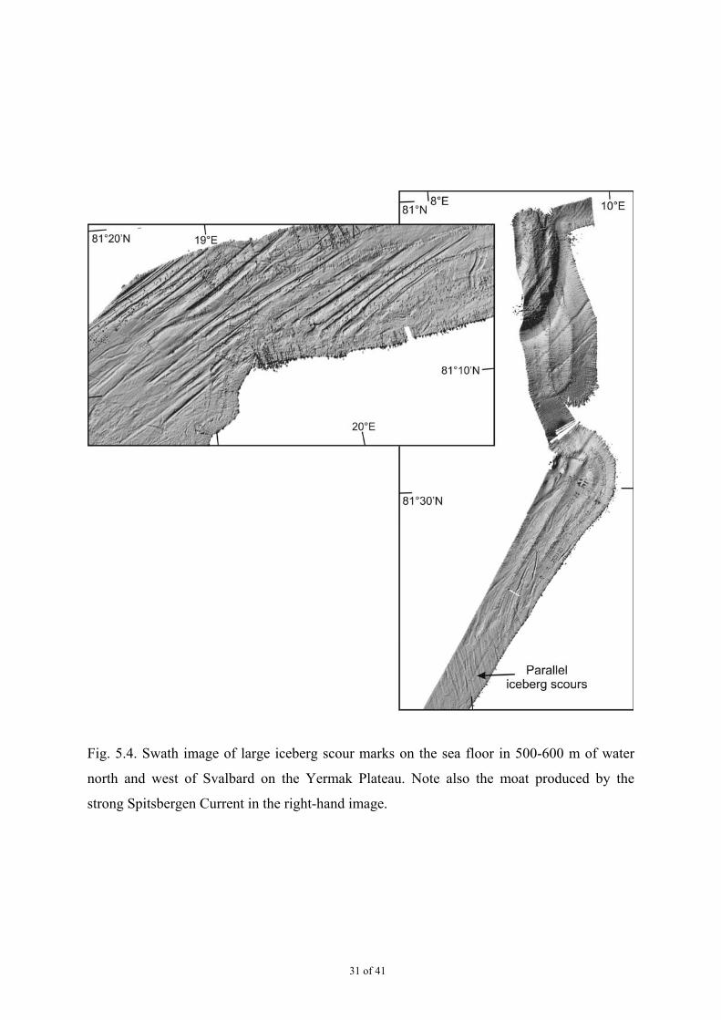
Fig. 5.4. Swath image of large iceberg scour marks on the sea floor in 500-600 m of water

north and west of Svalbard on the Yermak Plateau. Note also the moat produced by the

strong Spitsbergen Current in the right-hand image.

32 of 41

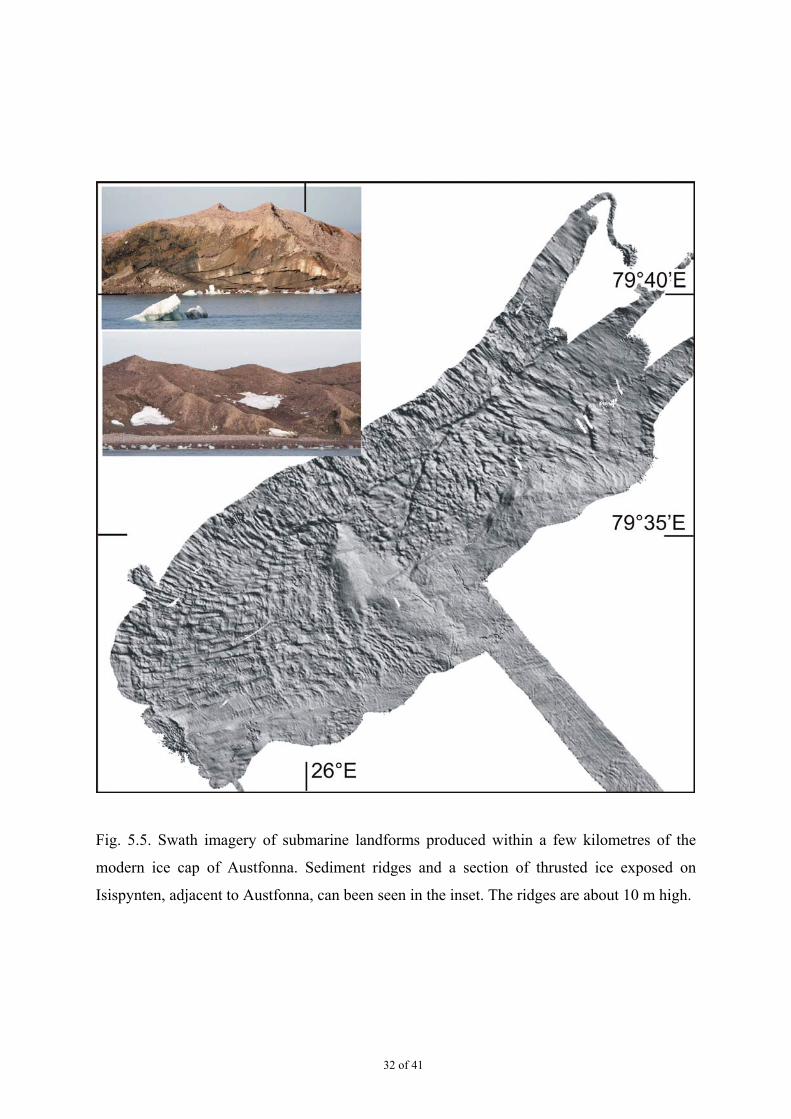
Fig. 5.5. Swath imagery of submarine landforms produced within a few kilometres of the

modern ice cap of Austfonna. Sediment ridges and a section of thrusted ice exposed on

Isispynten, adjacent to Austfonna, can been seen in the inset. The ridges are about 10 m high.

33 of 41

6. TESTS ON BACKSCATTER VALUES DERIVED FROM THE EM120(R. Noormets)

In some of the earlier swath data collected aboard JCR, abrupt changes in backscatter (BS)levels have been observed. The cause for these “jumps” is not fully understood.

During the JR142 cruise, series of tests were conducted with the aim of clarifying the originof the BS fluctuations and to investigate the possibilities for improving the quality of BS datacollected with the EM120.

The tests included:1. Calculating and implementing new acoustic energy absorption profiles appropriate for

local conditions using echosounder and water column parameters readily available onJCR.

2. Examining the effect of different factory preset operation modes on the output BSlevels.

1: A new absorption profile was calculated based on the equations given in the EM120operator’s manual using the following parameters measured on the vessel: pH, temperature,salinity, sound velocity. Absorption coefficients in the new profile were locally up to 30%different from those in the “standard” one used before. Deviations were greatest in the upper(shallower) end of the profile.The original absorption profile file in Neptune $SHAREHOME directory was renamed from“absorption.coef.EM120” to “absorption.coef.EM120.original” and the newly calculatedprofile was copied to that directory and named “absorption.coef.EM120”.The effect of implementing the new absorption profile is difficult to assess at this time as thisrequires testing in well controlled conditions, and preferably repeating survey lines overpreviously known seabed types. Theoretically, improvement in returned backscatter levelsshould be expected.

2: During normal data collecting, the EM120 is run in automatic mode, which ensures‘optimum’ bottom detection in full ocean range. The automatic mode consists of 5 factorypreset ping modes, each of which is designed for optimum bottom detection in different depthand bottom conditions. These ping modes (Very shallow, Shallow, Medium, Deep and Verydeep) feature a set of various parameters, such as maximum range, swath angle, pulse lengthetc. When underway, the EM120 switches between the ping modes automatically, based onthe outcome of a series of bottom detection tests that it performs continuously on theincoming swath data.

We started the testing with an assumption that the abrupt changes in backscatter levelsobserved in several earlier datasets (e.g. Bellingshausen Sea) may have been the result of theautomatic switching from one ping mode to the next. Testing was conducted under normaldata collecting procedures during TOBI-survey, i.e. with vessel speeds around 2-4 kn.

One typical example of the effect of mode switching has been summarized in the figuresbelow. In this case, the vessel was proceeding from north to south, i.e. from deeper to

34 of 41

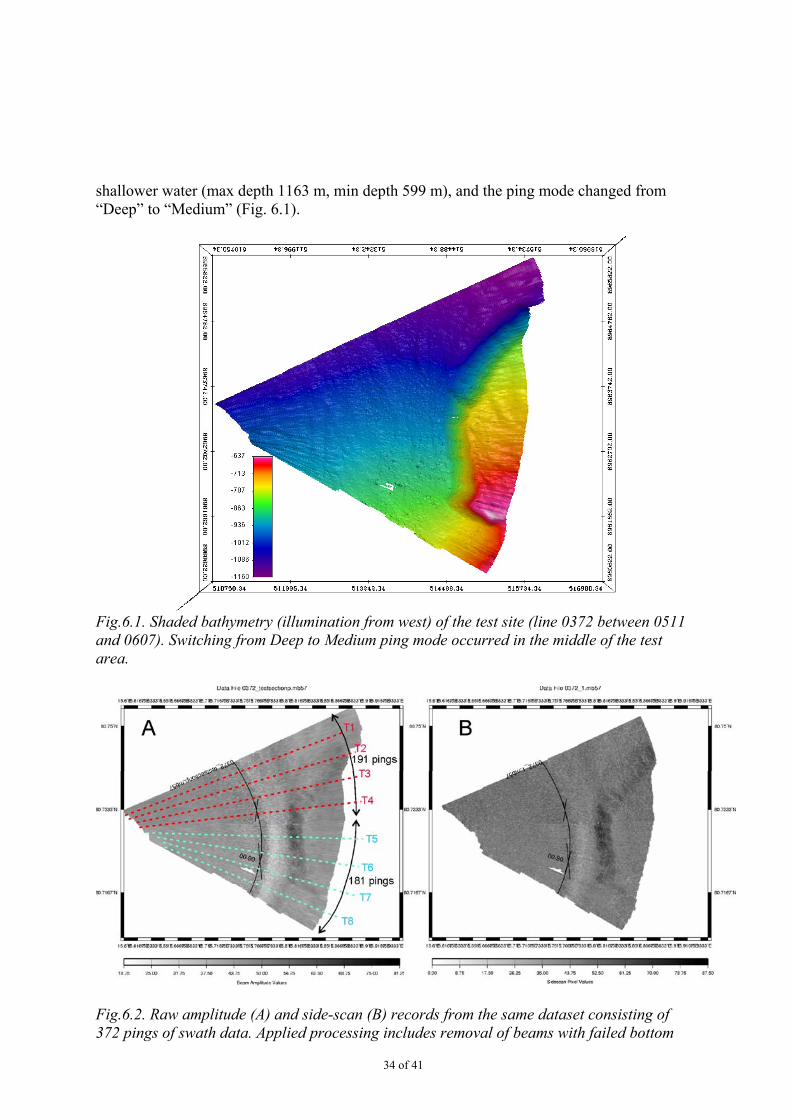
shallower water (max depth 1163 m, min depth 599 m), and the ping mode changed from“Deep” to “Medium” (Fig. 6.1).

Fig.6.1. Shaded bathymetry (illumination from west) of the test site (line 0372 between 0511and 0607). Switching from Deep to Medium ping mode occurred in the middle of the testarea.

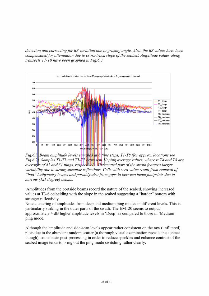
Fig.6.2. Raw amplitude (A) and side-scan (B) records from the same dataset consisting of372 pings of swath data. Applied processing includes removal of beams with failed bottom

35 of 41

detection and correcting for BS variation due to grazing angle. Also, the BS values have beencompensated for attenuation due to cross-track slope of the seabed. Amplitude values alongtransects T1-T8 have been graphed in Fig.6.3.

amp variation, from deep to medium, 50 ping avg. Xtrack slope & grazing angle corrected

20

25

30

35

40

45

50

55

60

65

70

1 51 101 151 201 251 301 351 401 451 501 551 601 651 701 751 801 851 901 951 1001swath angle, +/-66, 1024 cells

amp

T1_deepT2_deepT3_deepT4_deepT5_mediumT6_mediumT7_mediumT8_medium

Fig.6.3. Beam amplitude levels sampled at 8 time steps, T1-T8 (for approx. locations seeFig.6.2). Samples T1-T3 and T5-T7 represent 50 ping average values, whereas T4 and T8 areaverages of 41 and 31 pings, respectively. The central part of the swath features largervariability due to strong specular reflections. Cells with zero-value result from removal of“bad” bathymetry beams and possibly also from gaps in between beam footprints due tonarrow (1x1 degree) beams.

Amplitudes from the portside beams record the nature of the seabed, showing increasedvalues at T3-6 coinciding with the slope in the seabed suggesting a “harder” bottom withstronger reflectivity.Note clustering of amplitudes from deep and medium ping modes in different levels. This isparticularly striking in the outer parts of the swath. The EM120 seems to outputapproximately 4 dB higher amplitude levels in ‘Deep’ as compared to those in ‘Medium’ping mode.

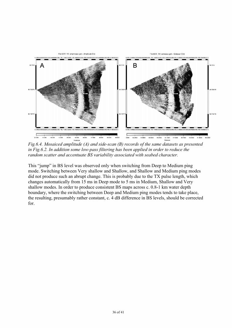
Although the amplitude and side-scan levels appear rather consistent on the raw (unfiltered)plots due to the abundant random scatter (a thorough visual examination reveals the contactthough), some basic post-processing in order to reduce speckles and enhance contrast of theseabed image tends to bring out the ping mode switching rather clearly.

36 of 41

Fig.6.4. Mosaiced amplitude (A) and side-scan (B) records of the same datasets as presentedin Fig.6.2. In addition some low-pass filtering has been applied in order to reduce therandom scatter and accentuate BS variability associated with seabed character.

This “jump” in BS level was observed only when switching from Deep to Medium pingmode. Switching between Very shallow and Shallow, and Shallow and Medium ping modesdid not produce such an abrupt change. This is probably due to the TX pulse length, whichchanges automatically from 15 ms in Deep mode to 5 ms in Medium, Shallow and Veryshallow modes. In order to produce consistent BS maps across c. 0.8-1 km water depthboundary, where the switching between Deep and Medium ping modes tends to take place,the resulting, presumably rather constant, c. 4 dB difference in BS levels, should be correctedfor.

37 of 41

7. APPENDICES

7.1 Sonar System Parameter Settings

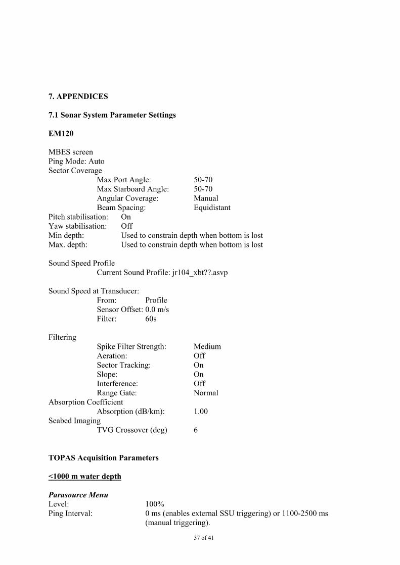
EM120

MBES screenPing Mode: AutoSector Coverage

Max Port Angle: 50-70Max Starboard Angle: 50-70Angular Coverage: ManualBeam Spacing: Equidistant

Pitch stabilisation: OnYaw stabilisation: OffMin depth: Used to constrain depth when bottom is lostMax. depth: Used to constrain depth when bottom is lost

Sound Speed ProfileCurrent Sound Profile: jr104_xbt??.asvp

Sound Speed at Transducer:From: ProfileSensor Offset: 0.0 m/sFilter: 60s

FilteringSpike Filter Strength: MediumAeration: OffSector Tracking: OnSlope: OnInterference: OffRange Gate: Normal

Absorption CoefficientAbsorption (dB/km): 1.00

Seabed ImagingTVG Crossover (deg) 6

TOPAS Acquisition Parameters

<1000 m water depth

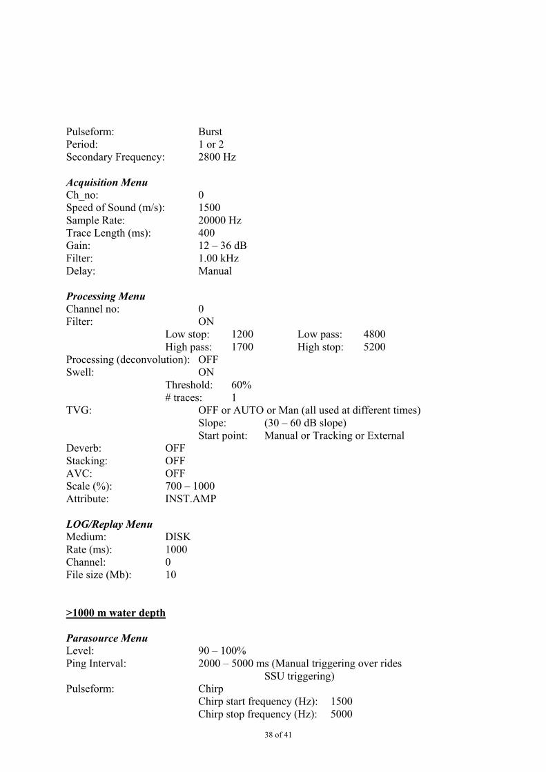
Parasource MenuLevel: 100%Ping Interval: 0 ms (enables external SSU triggering) or 1100-2500 ms

(manual triggering).

38 of 41

Pulseform: BurstPeriod: 1 or 2Secondary Frequency: 2800 Hz

Acquisition MenuCh_no: 0Speed of Sound (m/s): 1500Sample Rate: 20000 HzTrace Length (ms): 400Gain: 12 – 36 dBFilter: 1.00 kHzDelay: Manual

Processing MenuChannel no: 0Filter: ON

Low stop: 1200 Low pass: 4800High pass: 1700 High stop: 5200

Processing (deconvolution): OFFSwell: ON

Threshold: 60%# traces: 1

TVG: OFF or AUTO or Man (all used at different times)Slope: (30 – 60 dB slope)Start point: Manual or Tracking or External

Deverb: OFFStacking: OFFAVC: OFFScale (%): 700 – 1000Attribute: INST.AMP

LOG/Replay MenuMedium: DISKRate (ms): 1000Channel: 0File size (Mb): 10

>1000 m water depth

Parasource MenuLevel: 90 – 100%Ping Interval: 2000 – 5000 ms (Manual triggering over rides

SSU triggering)Pulseform: Chirp

Chirp start frequency (Hz): 1500Chirp stop frequency (Hz): 5000

39 of 41

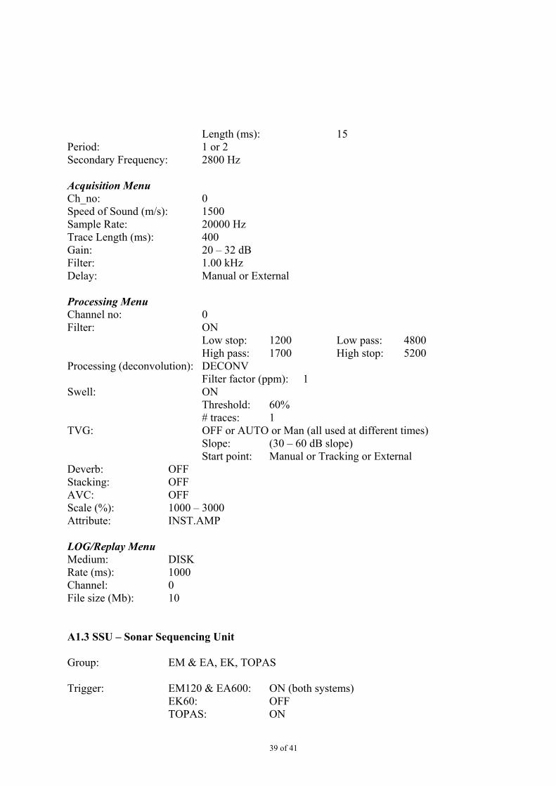
Length (ms): 15Period: 1 or 2Secondary Frequency: 2800 Hz

Acquisition MenuCh_no: 0Speed of Sound (m/s): 1500Sample Rate: 20000 HzTrace Length (ms): 400Gain: 20 – 32 dBFilter: 1.00 kHzDelay: Manual or External

Processing MenuChannel no: 0Filter: ON

Low stop: 1200 Low pass: 4800High pass: 1700 High stop: 5200

Processing (deconvolution): DECONVFilter factor (ppm): 1

Swell: ONThreshold: 60%# traces: 1

TVG: OFF or AUTO or Man (all used at different times)Slope: (30 – 60 dB slope)Start point: Manual or Tracking or External

Deverb: OFFStacking: OFFAVC: OFFScale (%): 1000 – 3000Attribute: INST.AMP

LOG/Replay MenuMedium: DISKRate (ms): 1000Channel: 0File size (Mb): 10

A1.3 SSU – Sonar Sequencing Unit

Group: EM & EA, EK, TOPAS

Trigger: EM120 & EA600: ON (both systems)EK60: OFFTOPAS: ON

40 of 41

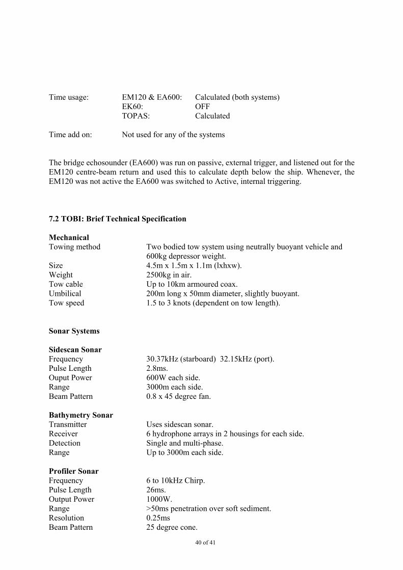
Time usage: EM120 & EA600: Calculated (both systems)EK60: OFFTOPAS: Calculated

Time add on: Not used for any of the systems

The bridge echosounder (EA600) was run on passive, external trigger, and listened out for theEM120 centre-beam return and used this to calculate depth below the ship. Whenever, theEM120 was not active the EA600 was switched to Active, internal triggering.

7.2 TOBI: Brief Technical Specification

MechanicalTowing method Two bodied tow system using neutrally buoyant vehicle and

600kg depressor weight.Size 4.5m x 1.5m x 1.1m (lxhxw).Weight 2500kg in air.Tow cable Up to 10km armoured coax.Umbilical 200m long x 50mm diameter, slightly buoyant.Tow speed 1.5 to 3 knots (dependent on tow length).

Sonar Systems

Sidescan SonarFrequency 30.37kHz (starboard) 32.15kHz (port).Pulse Length 2.8ms.Ouput Power 600W each side.Range 3000m each side.Beam Pattern 0.8 x 45 degree fan.

Bathymetry SonarTransmitter Uses sidescan sonar.Receiver 6 hydrophone arrays in 2 housings for each side.Detection Single and multi-phase.Range Up to 3000m each side.

Profiler SonarFrequency 6 to 10kHz Chirp.Pulse Length 26ms.Output Power 1000W.Range >50ms penetration over soft sediment.Resolution 0.25msBeam Pattern 25 degree cone.

41 of 41

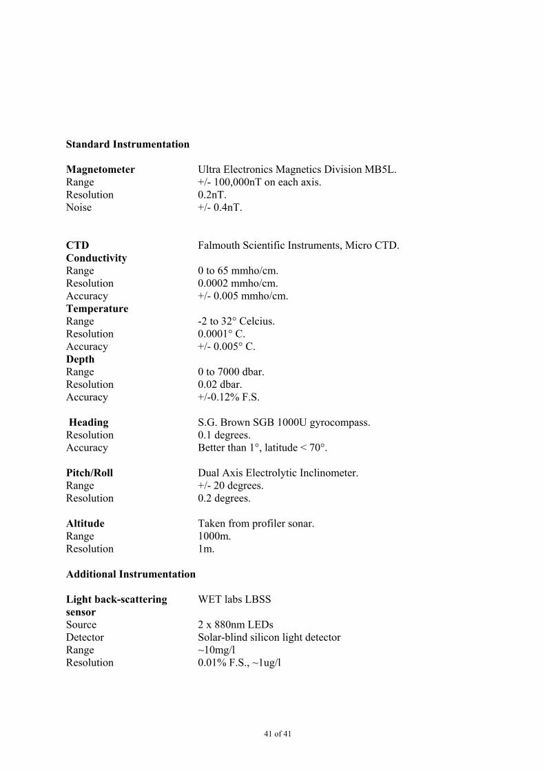
Standard Instrumentation

Magnetometer Ultra Electronics Magnetics Division MB5L.Range +/- 100,000nT on each axis.Resolution 0.2nT.Noise +/- 0.4nT.

CTD Falmouth Scientific Instruments, Micro CTD.ConductivityRange 0 to 65 mmho/cm.Resolution 0.0002 mmho/cm.Accuracy +/- 0.005 mmho/cm.Temperature Range -2 to 32° Celcius.Resolution 0.0001° C.Accuracy +/- 0.005° C.DepthRange 0 to 7000 dbar.Resolution 0.02 dbar.Accuracy +/-0.12% F.S.

Heading S.G. Brown SGB 1000U gyrocompass.Resolution 0.1 degrees.Accuracy Better than 1°, latitude < 70°.

Pitch/Roll Dual Axis Electrolytic Inclinometer.Range +/- 20 degrees.Resolution 0.2 degrees.

Altitude Taken from profiler sonar.Range 1000m.Resolution 1m.

Additional Instrumentation

Light back-scattering WET labs LBSSsensorSource 2 x 880nm LEDsDetector Solar-blind silicon light detectorRange ~10mg/lResolution 0.01% F.S., ~1ug/l