Crustal Structure, Crustal Earthquake Process and

Earthquake StrongGround Motion Scaling for the

Conterminous U.S.

R. B. HerrmannOtto Nuttli Professor of Geophysics

Saint Louis University

Interrelated Studies• Ground motion study requires

• Moment magnitude for absolute calibration, which is determined from

• Source mechanism, depth and moment determination, which needs

• Crustal structure, from• Receiver functions and • Surface wave dispersion

Earthquake Focal Mechanism Determination

• First motion– need high quality data– need good sampling of focal sphere

• Waveform modeling– good waveforms - high S/N– good crustal model

• Spectral amplitudes

Procedure

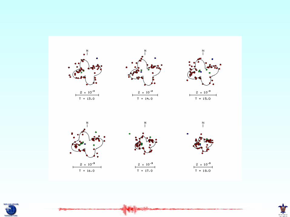
• Multiple filter analysis to define spectral amplitudes

• Radiation pattern search for 4 possible mechanisms (180 degree symmetry and P-T axis switch)

• Select according to waveform prediction or good first motion

Timeline

• All digital data in hand within 1 hour of event - 70 Mb downloaded

• Data QC, spectral analysis, grid search, forward modeling, web page generation within 1 hour

Evansville - 18 JUN 2002Mw = 4.57

Questions

• Can procedure be fully automated?

• Can timeline be shortened• Can direct waveform inversion be

made less sensitive to velocity model• What patterns are emerging

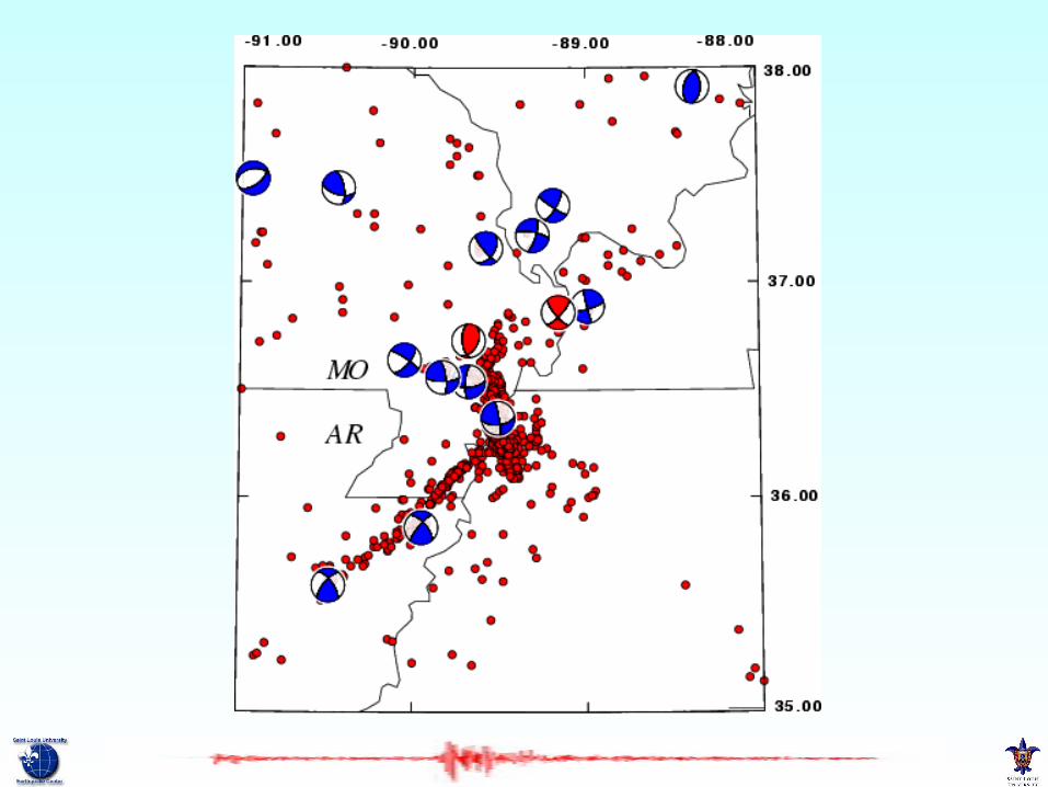
Focal Mechanisms

Red (2004). Shaded quadrants are compressions (tension quadrant)

Tension Axis Trend

Red (2004). Plot of projection of tension axis on horizontal - longest correspond to axis with 0 plunge

Pressure Axis Trend

Red (2004). Plot of projection of pressure axis on horizontal - longest correspond to axis with 0 plunge

Direction of Maximum Compressive Stress (Zoback, 1992)

Questions

• Why does nature of focal mechanism change

• What is relation to pattern of seismicity, especially location of larger earthquakes

Current work

• Systematically determining mechanisms using USNSN digital data from 1990 - present.

• Determining lower magnitude limit as function of network geometry and time of year (S/N)

Issues in High FrequencyGround Motion Scaling:Regression, Crust, Absolute

Scaling

Objective of Studies

• Construct a forward ground motion model for a region using– Recordings of small and large

earthquakes– Tool of random vibration theory /

stochastic simulation

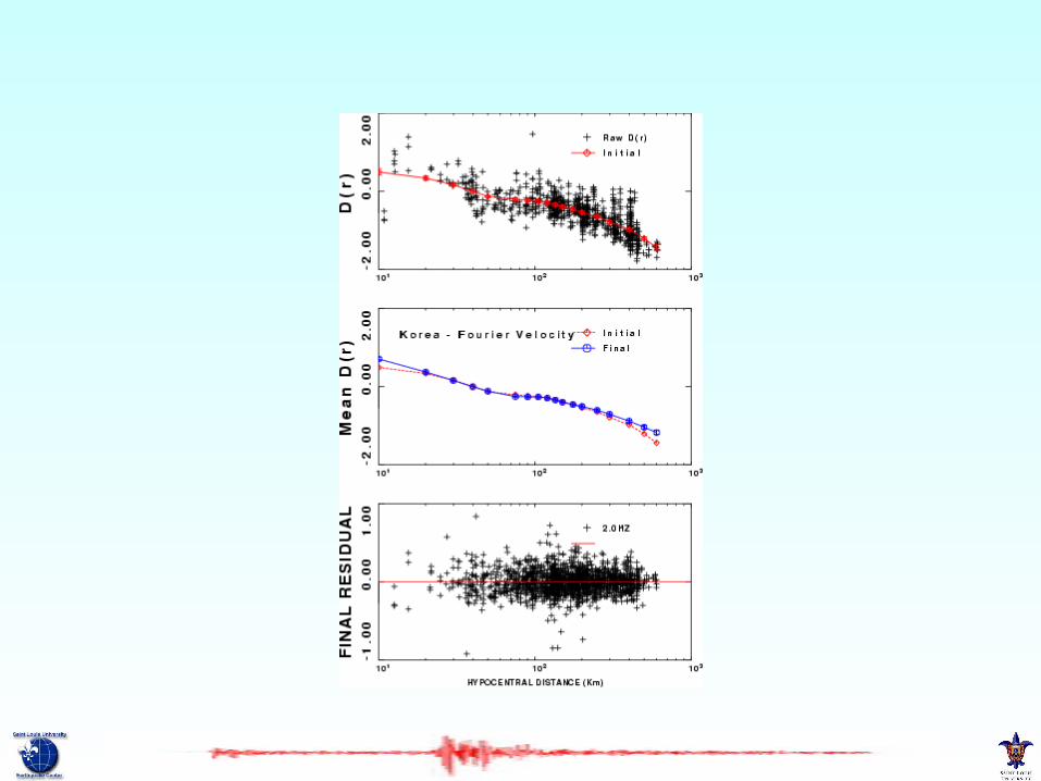
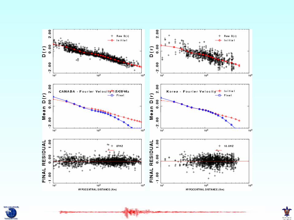
Regression

• Data from small earthquakes

• Model

A = E + D + SA = log a

E = excitation (not source)

D = distance

S = site

Interpretation - Model

• Has physicssource, propagation, site

• What is relation to regression?

• Interpretation indicates procedure– propagation– site– source

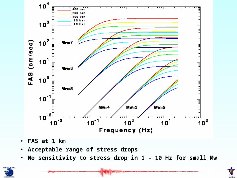
• FAS at 1 km

• Acceptable range of stress drops• No sensitivity to stress drop in 1 - 10 Hz for small Mw

Questions

• Is a study of vertical component motions useful for predicting horizontal motions?

• What is the nature of the ground motion scaling from the source to the first observation point? Does this depend upon the focal mechanism?

• How does crustal structure affect ground motions, especially at larger distances?

• Does the simple forward prediction model apply to all frequencies

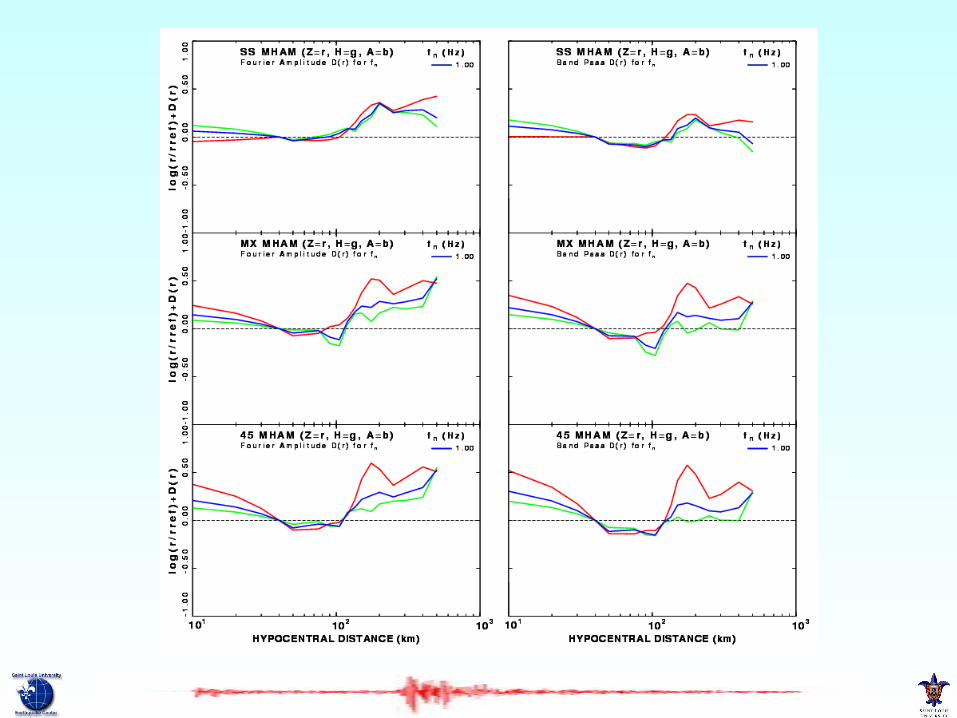
Method

• Create data set with synthetics– 240 events, 23 stations (15000)

• Use different velocity models• Use different focal mechanisms– Strike slip– 45 dip slip– mix of strike slip and dip slip

• Process as with real data

• Compare mechanism effect for different models at 1.0 Hz

• Examination excitation• Look at Excitation

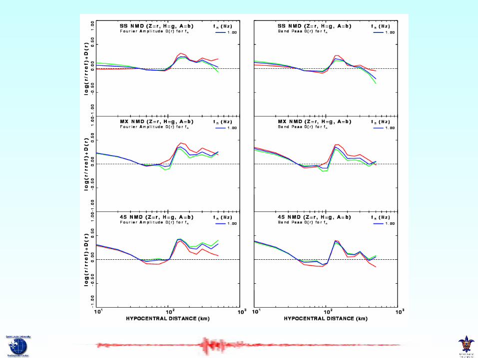
Summary

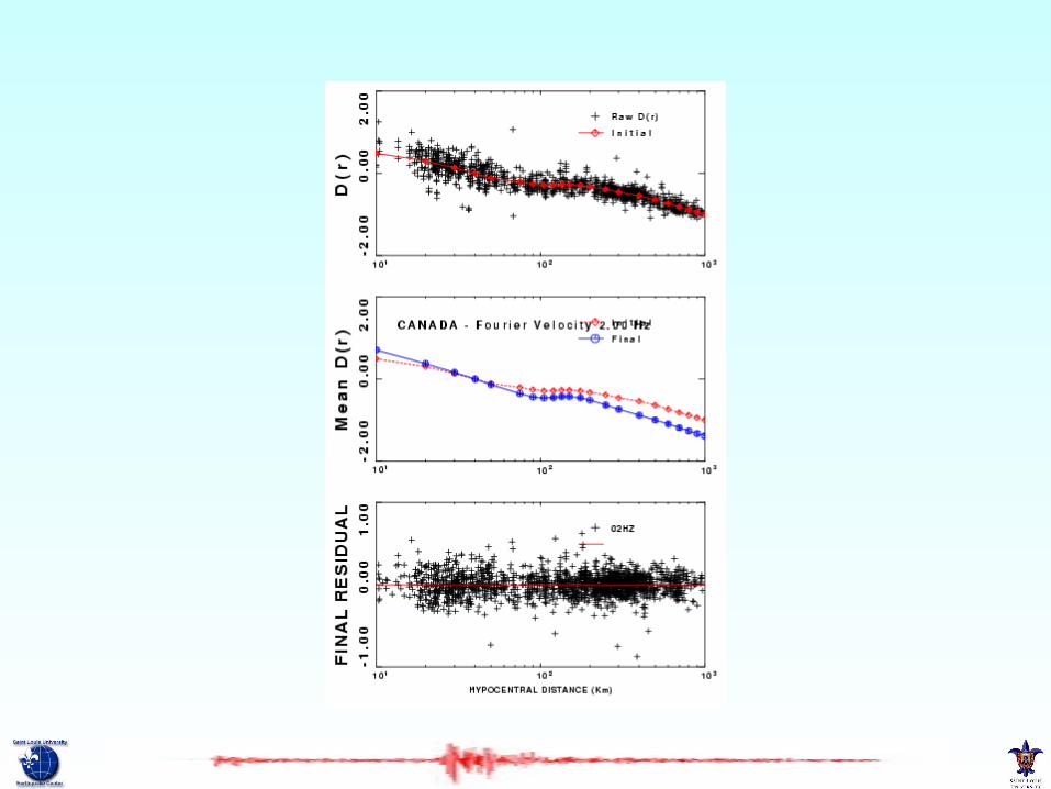
• Crustal thickness affects motion at large distance - e.g., where 1st super critical reflection arrives

• Regression on different components gives very different D( r ) at short distance– NWIT had low Q in crust– NMD had low Q in sediment

Conclusions

• Nothing sacred about 1/R from source

• Relation between source radiation and ‘n’ in R-n

Methodolody

• Data Reduction

• Regression • Fit Fourier Spectra• Fit Peak Velocity• TEST g( r) near source by comparing

observed spectra for Mw=4 to predicted (requires waveform Mw estimate)

Implications

• Different strong ground motion scaling relations expected at short distances for different parts of the US according to regional earthquake process - strike-slip vs thrust or normal faulting

Opportunities

• EarthScope– USArray

• Advanced National Seismic System

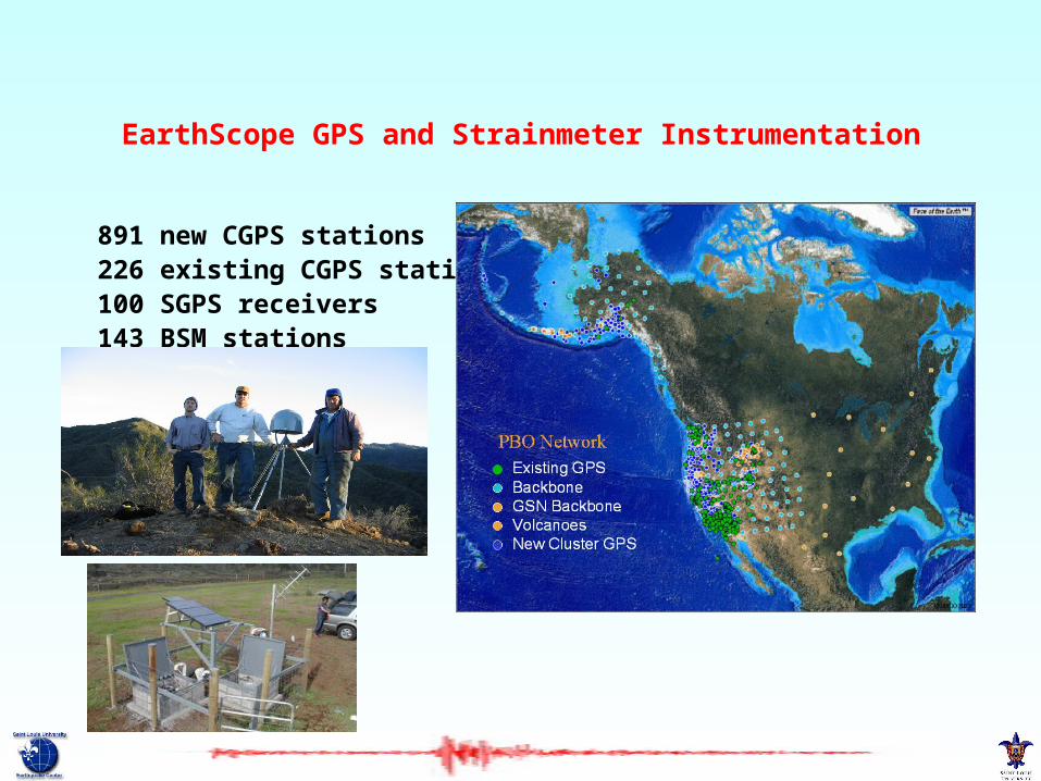
EarthScope GPS and Strainmeter Instrumentation

891 new CGPS stations226 existing CGPS stations100 SGPS receivers143 BSM stations 5 LSM stations

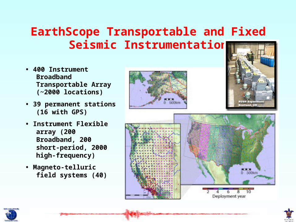
EarthScope Transportable and Fixed Seismic Instrumentation

• 400 Instrument Broadband Transportable Array (~2000 locations)

• 39 permanent stations (16 with GPS)

• Instrument Flexible array (200 Broadband, 200 short-period, 2000 high-frequency)

• Magneto-telluric field systems (40)

USArray – "Bigfoot"

• 400 broadband seismometers– 70 km spacing– Nominal 1400 x 1400 km

grid

• 50 magnetotelluric field systems

• Deployments for ~18 months at each site

• Rolling deployment over ~ 10 years

My Research Directions

• USArray Data– map focal mechanisms (only about 10-

20 annually with Mw > 4 outside California - more if lower threshold

– define S-velocity structure of upper crust - needed for inversion of waveforms

– characterize regional high frequency ground motion scaling

Computer Programs in Seismology

Version 3.30

• UNIX

• LINUX• MacOSX• Windows– Cygwin (100%)

– Zhao and Helmberger, Zhu and Helmberger waveform

inversion

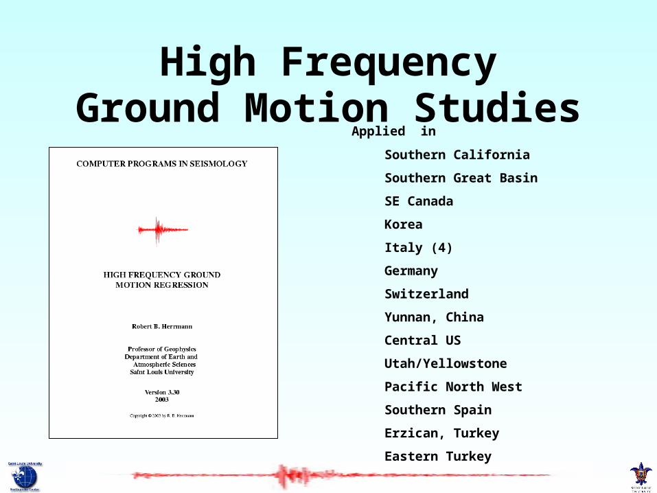
High FrequencyGround Motion Studies

Applied in

Southern California

Southern Great Basin

SE Canada

Korea

Italy (4)

Germany

Switzerland

Yunnan, China

Central US

Utah/Yellowstone

Pacific North West

Southern Spain

Erzican, Turkey

Eastern Turkey

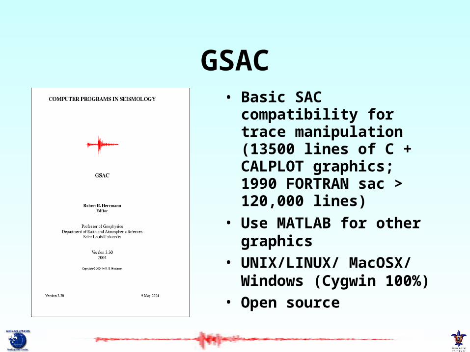
GSAC• Basic SAC compatibility

for trace manipulation (13500 lines of C + CALPLOT graphics; 1990 FORTRAN sac > 120,000 lines)

• Use MATLAB for other graphics

• UNIX/LINUX/ MacOSX/ Windows (Cygwin 100%)

• Open source

Version 3.35

• Transverse Isotropy – surface wave modeling– surface wave inversion

• Shallow S-wave velocity determination – SPAC, ESAC– Joint inversion of refraction survey

dispersion and first arrivals

The BOOK

300 pages typeset so far

Caveats (concerns)

• Equation is not uniqueA = ( E + 1 ) + ( D - 1 ) + S

one event is only data in one distance range

A = E + ( D - 1 ) + ( S + 1 )one station provides data in one distance range

• Thus constraintsD(rref ) = 0 , and Σ S = 0