1

CS 188: Artificial Intelligence

Lectures 2 and 3: Search

Pieter Abbeel – UC Berkeley

Many slides from Dan Klein

Reminder

§  Only a very small fraction of AI is about making computers play games intelligently

§  Recall: computer vision, natural language, robotics, machine learning, computational biology, etc.

§  That being said: games tend to provide relatively simple example settings which are great to illustrate concepts and learn about algorithms which underlie many areas of AI

2

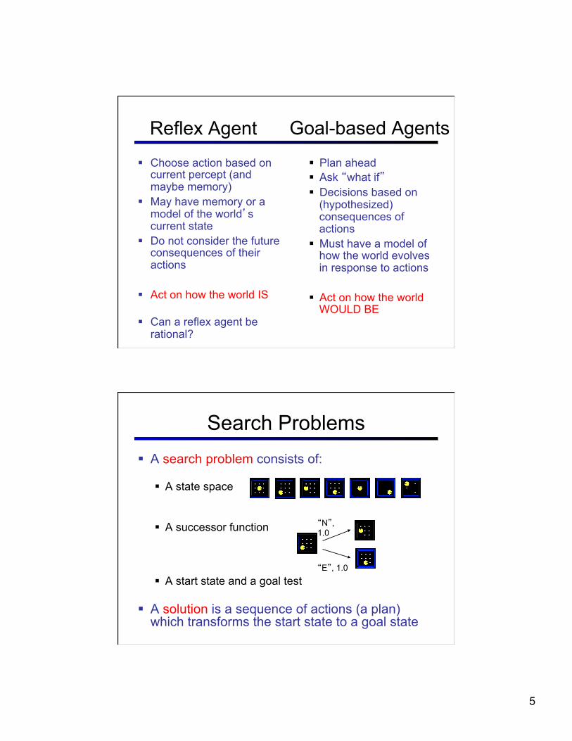
Reflex Agent

§  Choose action based on current percept (and maybe memory)

§  May have memory or a model of the world’s current state

§  Do not consider the future consequences of their actions

§  Act on how the world IS

§  Can a reflex agent be rational?

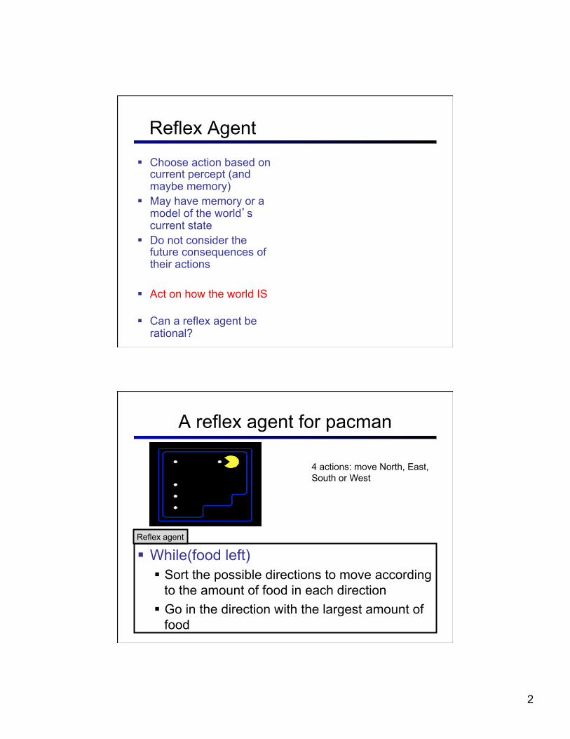
A reflex agent for pacman

§  While(food left) §  Sort the possible directions to move according

to the amount of food in each direction § Go in the direction with the largest amount of

food

Reflex agent

4 actions: move North, East, South or West

3

A reflex agent for pacman (2)

§  While(food left) §  Sort the possible directions to move according

to the amount of food in each direction § Go in the direction with the largest amount of

food

Reflex agent

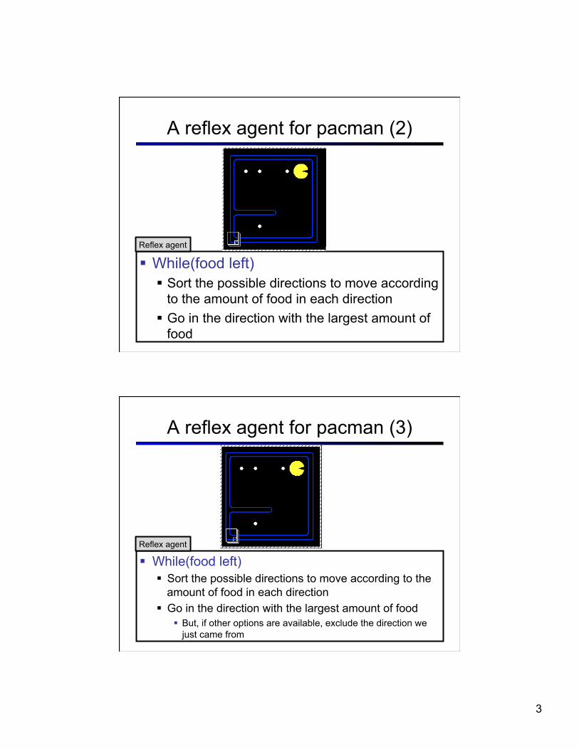
A reflex agent for pacman (3)

§  While(food left) §  Sort the possible directions to move according to the

amount of food in each direction §  Go in the direction with the largest amount of food

§  But, if other options are available, exclude the direction we just came from

Reflex agent

4

A reflex agent for pacman (4)

§  While(food left) §  If can keep going in the current direction, do so §  Otherwise:

§  Sort directions according to the amount of food §  Go in the direction with the largest amount of food §  But, if other options are available, exclude the direction we just

came from

Reflex agent

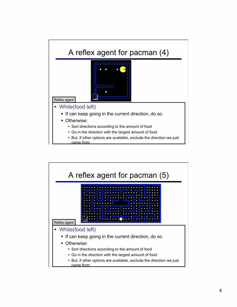
A reflex agent for pacman (5)

§  While(food left) §  If can keep going in the current direction, do so §  Otherwise:

§  Sort directions according to the amount of food §  Go in the direction with the largest amount of food §  But, if other options are available, exclude the direction we just

came from

Reflex agent

5

Reflex Agent

§  Choose action based on current percept (and maybe memory)

§  May have memory or a model of the world’s current state

§  Do not consider the future consequences of their actions

§  Act on how the world IS

§  Can a reflex agent be rational?

§  Plan ahead §  Ask “what if” §  Decisions based on

(hypothesized) consequences of actions

§  Must have a model of how the world evolves in response to actions

§  Act on how the world WOULD BE

Goal-based Agents

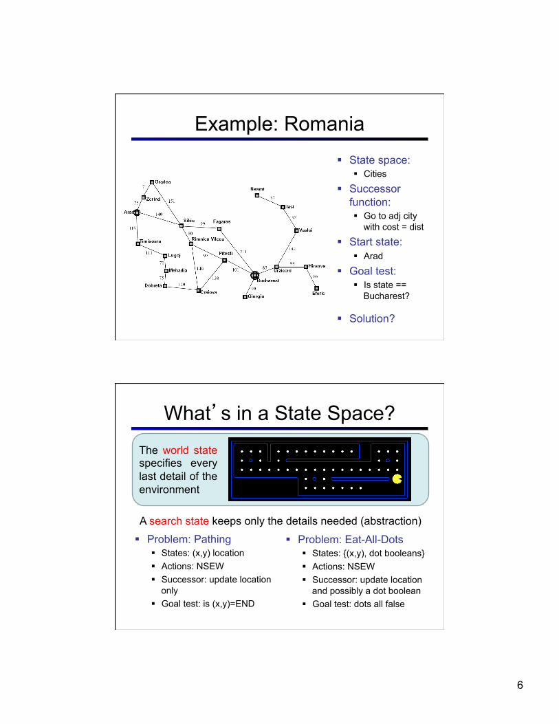
Search Problems §  A search problem consists of:

§  A state space

§  A successor function

§  A start state and a goal test

§  A solution is a sequence of actions (a plan) which transforms the start state to a goal state

“N”, 1.0

“E”, 1.0

6

Example: Romania §  State space:

§  Cities

§  Successor function: §  Go to adj city

with cost = dist

§  Start state: §  Arad

§  Goal test: §  Is state ==

Bucharest?

§  Solution?

What’s in a State Space?

§  Problem: Pathing §  States: (x,y) location §  Actions: NSEW §  Successor: update location

only §  Goal test: is (x,y)=END

§  Problem: Eat-All-Dots §  States: {(x,y), dot booleans} §  Actions: NSEW §  Successor: update location

and possibly a dot boolean §  Goal test: dots all false

The world state specifies every last detail of the environment

A search state keeps only the details needed (abstraction)

7

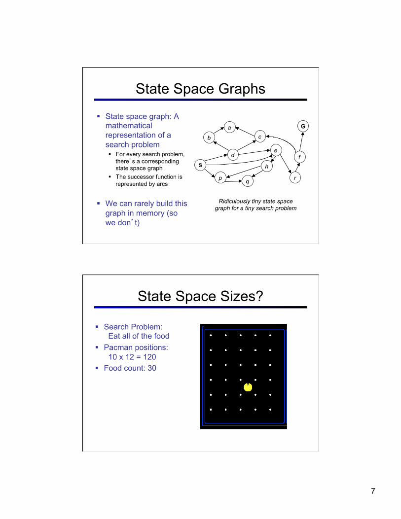
State Space Graphs

§  State space graph: A mathematical representation of a search problem §  For every search problem,

there’s a corresponding state space graph

§  The successor function is represented by arcs

§  We can rarely build this graph in memory (so we don’t)

S

G

d

b

p q

c

e

h

a

f

r

Ridiculously tiny state space graph for a tiny search problem

State Space Sizes?

§  Search Problem: Eat all of the food

§  Pacman positions: 10 x 12 = 120

§  Food count: 30 §  Ghost positions: 12 §  Pacman facing:

up, down, left, right

8

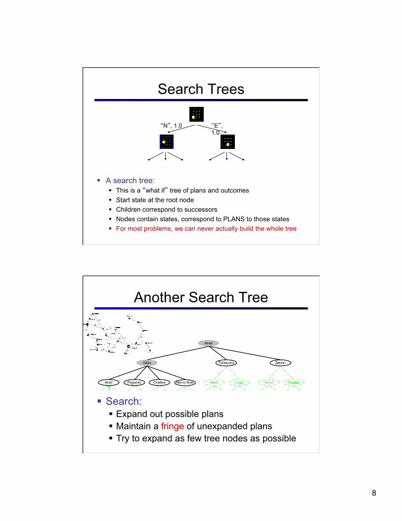
Search Trees

§  A search tree: §  This is a “what if” tree of plans and outcomes §  Start state at the root node §  Children correspond to successors §  Nodes contain states, correspond to PLANS to those states §  For most problems, we can never actually build the whole tree

“E”, 1.0

“N”, 1.0

Another Search Tree

§  Search: §  Expand out possible plans § Maintain a fringe of unexpanded plans §  Try to expand as few tree nodes as possible

9

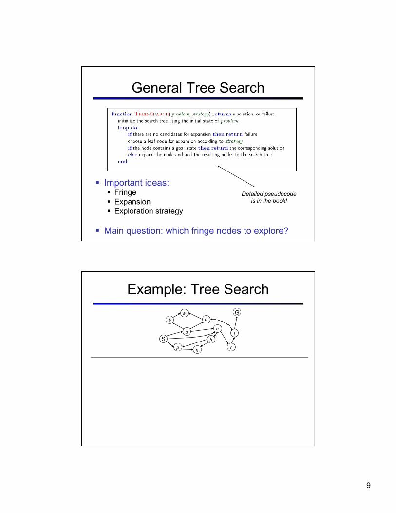
General Tree Search

§  Important ideas: §  Fringe §  Expansion §  Exploration strategy

§  Main question: which fringe nodes to explore?

Detailed pseudocode is in the book!

Example: Tree Search

S

G

d

b

p q

c

e

h

a

f

r

10

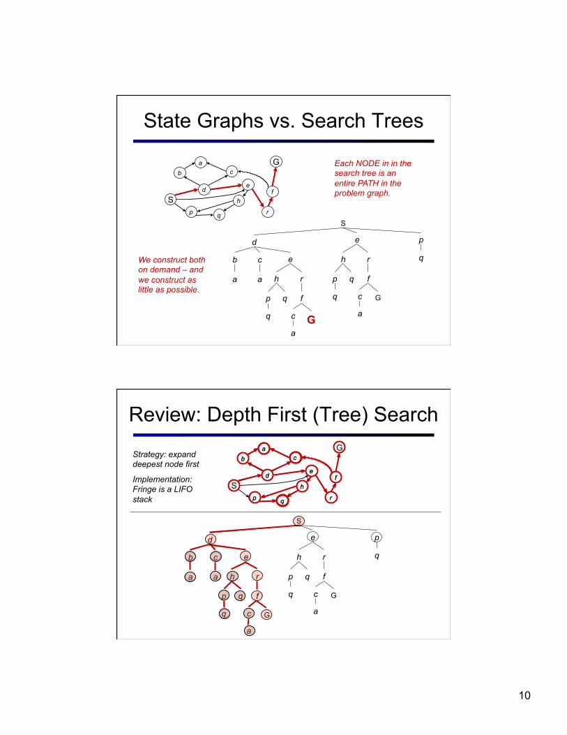
State Graphs vs. Search Trees

S

a

b

d p

a

c

e

p

h

f

r

q

q c G

a

q e

p

h

f

r

q

q c G a

S

G

d

b

p q

c

e

h

a

f

r

We construct both on demand – and we construct as little as possible.

Each NODE in in the search tree is an entire PATH in the problem graph.

Review: Depth First (Tree) Search

S

a

b

d p

a

c

e

p

h

f

r

q

q c G

a

q e

p

h

f

r

q

q c G

a

S

G

d

b

p q

c

e

h

a

f

r q p

h f d

b a

c

e

r

Strategy: expand deepest node first

Implementation: Fringe is a LIFO stack

11

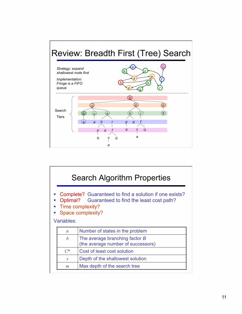
Review: Breadth First (Tree) Search

S

a

b

d p

a

c

e

p

h

f

r

q

q c G

a

q e

p

h

f

r

q

q c G

a

S

G

d

b

p q

c e

h

a

f

r

Search

Tiers

Strategy: expand shallowest node first

Implementation: Fringe is a FIFO queue

Search Algorithm Properties

§  Complete? Guaranteed to find a solution if one exists? §  Optimal? Guaranteed to find the least cost path? §  Time complexity? §  Space complexity?

Variables:

n Number of states in the problem b The average branching factor B

(the average number of successors) C* Cost of least cost solution s Depth of the shallowest solution m Max depth of the search tree

12

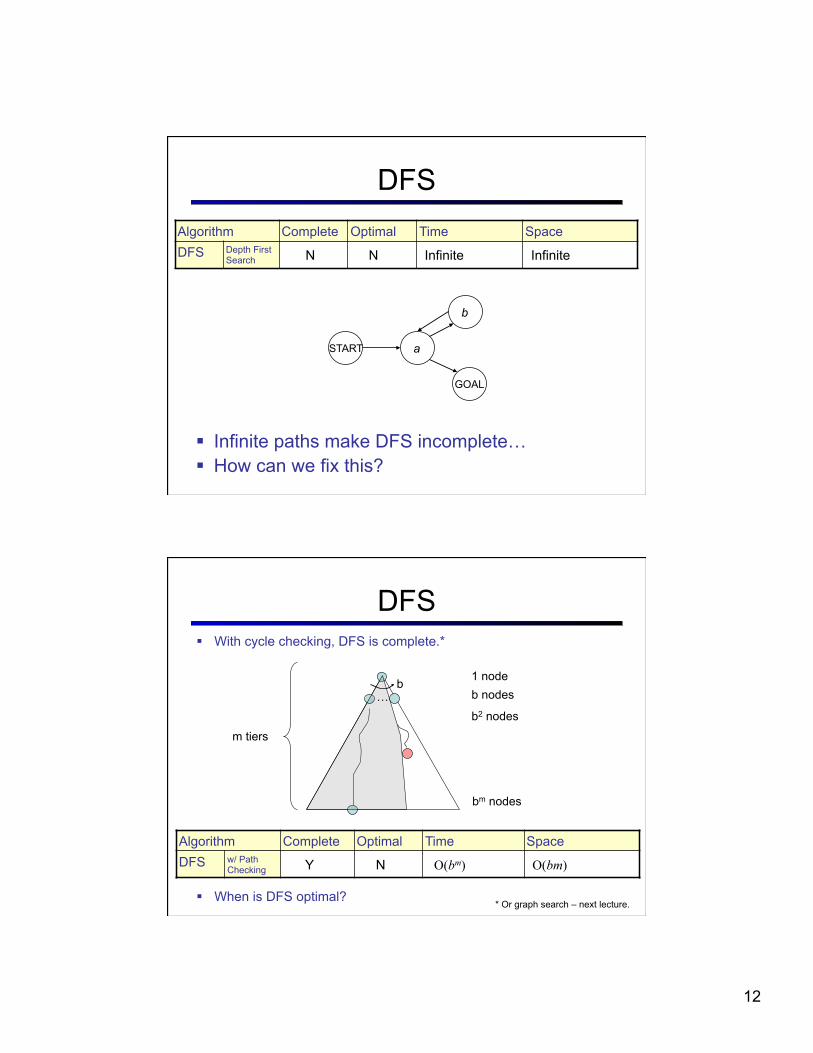
DFS

§  Infinite paths make DFS incomplete… §  How can we fix this?

Algorithm Complete Optimal Time Space DFS Depth First

Search N N O(BLMAX) O(LMAX)

START

GOAL

a

b

N N Infinite Infinite

DFS §  With cycle checking, DFS is complete.*

§  When is DFS optimal?

Algorithm Complete Optimal Time Space DFS w/ Path

Checking Y N O(bm) O(bm)

…b 1 node

b nodes

b2 nodes

bm nodes

m tiers

* Or graph search – next lecture.

13

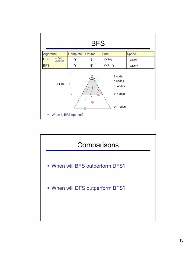
BFS

§  When is BFS optimal?

Algorithm Complete Optimal Time Space DFS w/ Path

Checking

BFS

Y N O(bm) O(bm)

…b 1 node

b nodes

b2 nodes

bm nodes

s tiers

Y N* O(bs+1) O(bs+1)

bs nodes

Comparisons

§  When will BFS outperform DFS?

§  When will DFS outperform BFS?

14

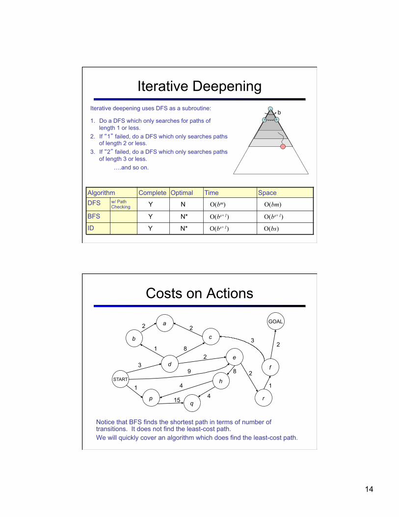
Iterative Deepening Iterative deepening uses DFS as a subroutine:

1.  Do a DFS which only searches for paths of length 1 or less.

2.  If “1” failed, do a DFS which only searches paths of length 2 or less.

3.  If “2” failed, do a DFS which only searches paths of length 3 or less. ….and so on.

Algorithm Complete Optimal Time Space DFS w/ Path

Checking

BFS

ID

Y N O(bm) O(bm)

Y N* O(bs+1) O(bs+1)

Y N* O(bs+1) O(bs)

…b

Costs on Actions

Notice that BFS finds the shortest path in terms of number of transitions. It does not find the least-cost path. We will quickly cover an algorithm which does find the least-cost path.

START

GOAL

d

b

p q

c

e

h

a

f

r

2

9 2

8 1

8

2

3

1

4

4

15

1

3 2

2

15

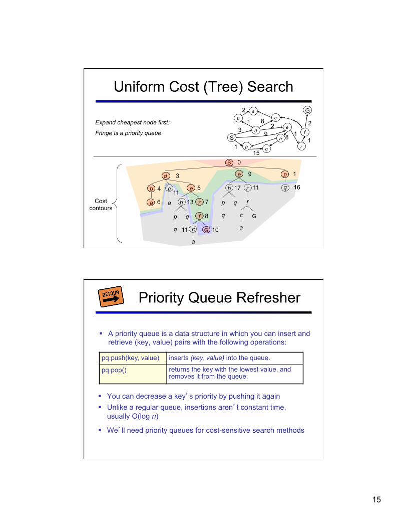
Uniform Cost (Tree) Search

S

a

b

d p

a

c

e

p

h

f

r

q

q c G

a

q e

p

h

f

r

q

q c G

a

Expand cheapest node first:

Fringe is a priority queue S

G

d

b

p q

c

e

h

a

f

r

3 9 1

16 4 11

5

7 13

8

10 11

17 11

0

6

3 9

1

1

2

8

8 1

15

1

2

Cost contours

2

Priority Queue Refresher

pq.push(key, value) inserts (key, value) into the queue.

pq.pop() returns the key with the lowest value, and removes it from the queue.

§  You can decrease a key’s priority by pushing it again §  Unlike a regular queue, insertions aren’t constant time,

usually O(log n)

§  We’ll need priority queues for cost-sensitive search methods

§  A priority queue is a data structure in which you can insert and retrieve (key, value) pairs with the following operations:

16

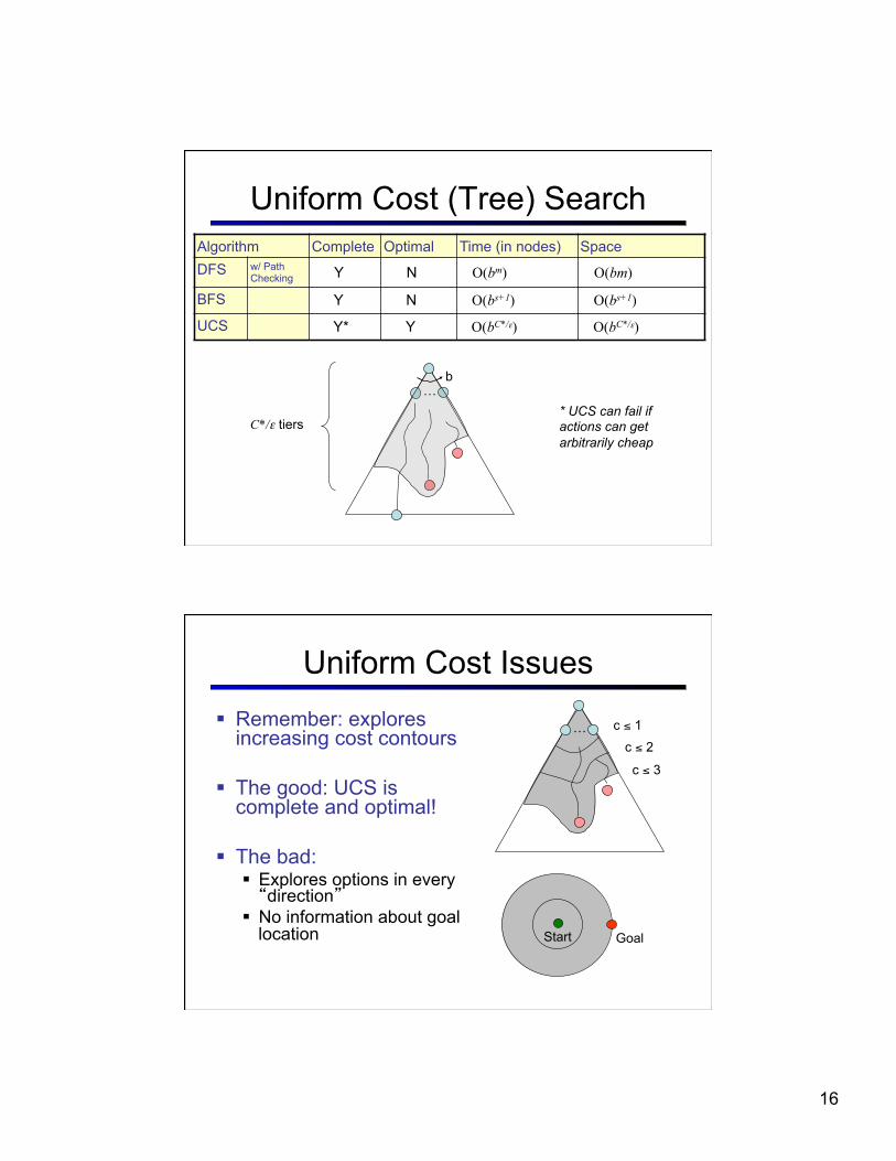
Uniform Cost (Tree) Search Algorithm Complete Optimal Time (in nodes) Space DFS w/ Path

Checking

BFS

UCS

Y N O(bm) O(bm)

…b

C*/ε tiers

Y N O(bs+1) O(bs+1)

Y* Y O(bC*/ε) O(bC*/ε)

* UCS can fail if actions can get arbitrarily cheap

Uniform Cost Issues §  Remember: explores

increasing cost contours

§  The good: UCS is complete and optimal!

§  The bad: §  Explores options in every “direction”

§  No information about goal location Start Goal

…

c ≤ 3

c ≤ 2 c ≤ 1

17

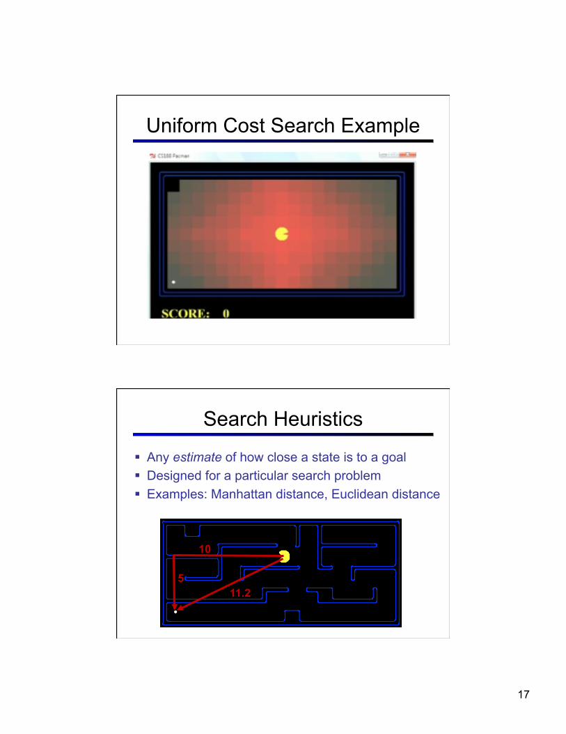
Uniform Cost Search Example

Search Heuristics

§  Any estimate of how close a state is to a goal §  Designed for a particular search problem §  Examples: Manhattan distance, Euclidean distance

10

5 11.2

18

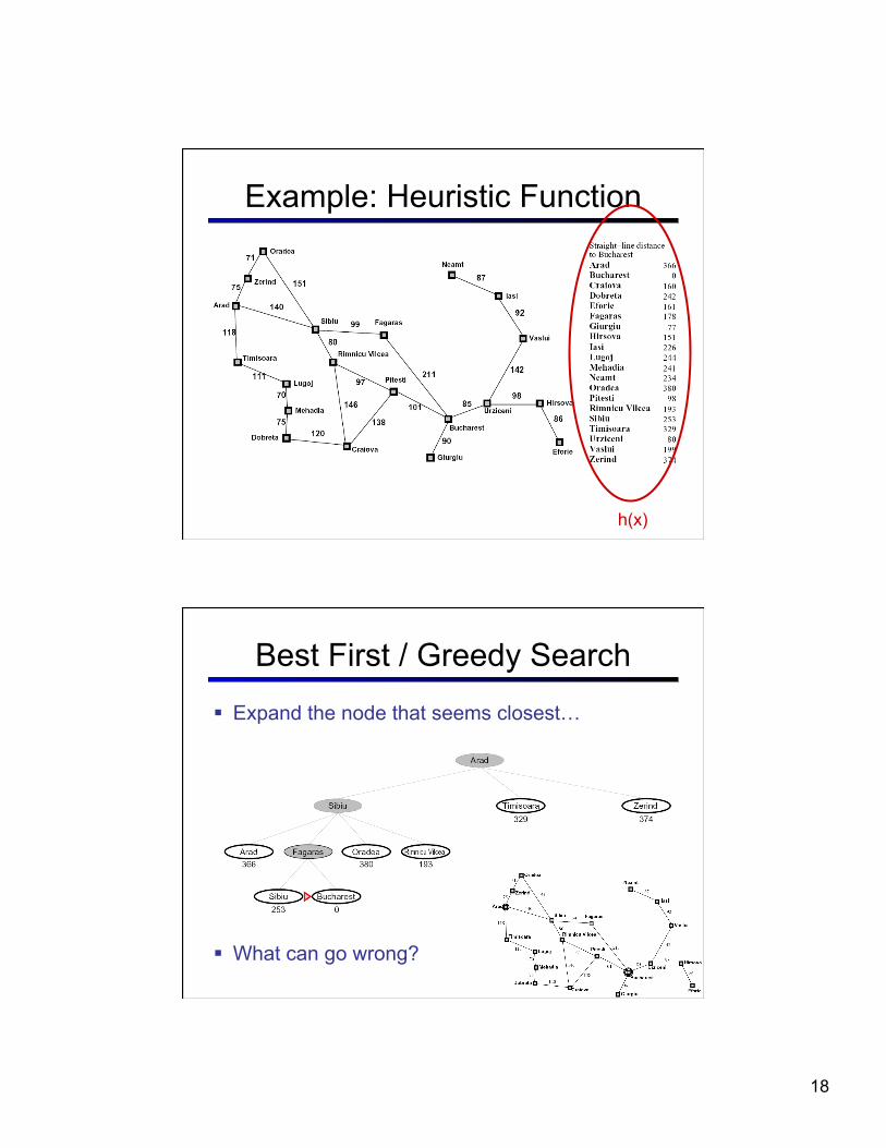
Example: Heuristic Function

h(x)

Best First / Greedy Search

§  Expand the node that seems closest…

§  What can go wrong?

19

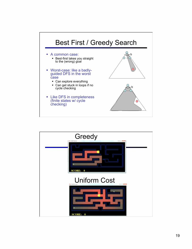
Best First / Greedy Search §  A common case:

§  Best-first takes you straight to the (wrong) goal

§  Worst-case: like a badly-guided DFS in the worst case §  Can explore everything §  Can get stuck in loops if no

cycle checking

§  Like DFS in completeness (finite states w/ cycle checking)

…b

…b

Uniform Cost

Greedy

20

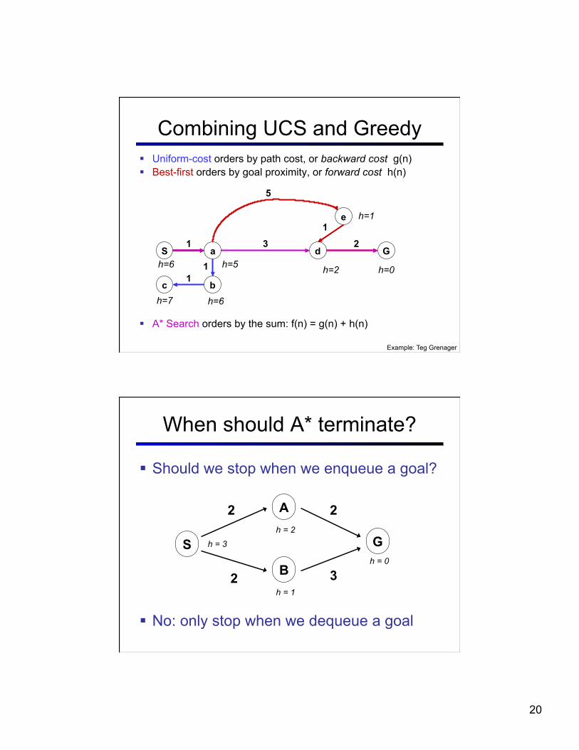
Combining UCS and Greedy §  Uniform-cost orders by path cost, or backward cost g(n) §  Best-first orders by goal proximity, or forward cost h(n)

§  A* Search orders by the sum: f(n) = g(n) + h(n)

S a d

b

G h=5

h=6

h=2

1

5

1 1

2

h=6 h=0 c

h=7

3

e h=1 1

Example: Teg Grenager

§  Should we stop when we enqueue a goal?

§  No: only stop when we dequeue a goal

When should A* terminate?

S

B

A

G

2

3

2

2 h = 1

h = 2

h = 0

h = 3

21

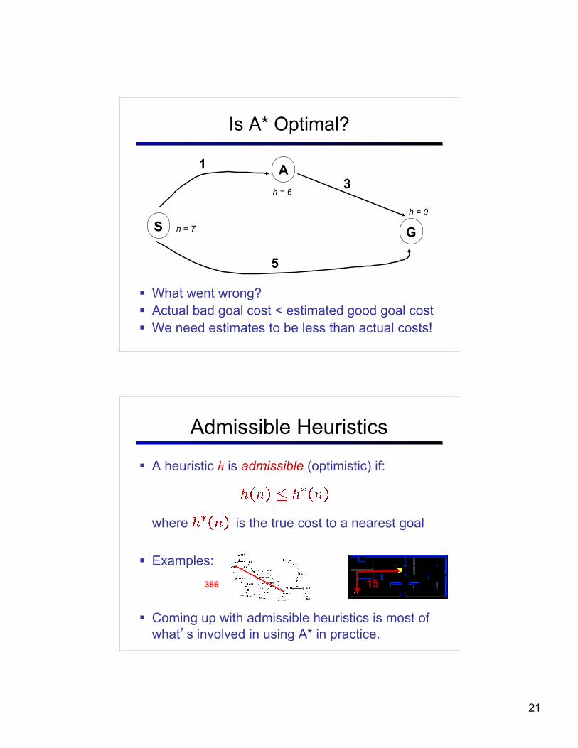
Is A* Optimal?

A

G S

1 3

h = 6

h = 0

5

h = 7

§  What went wrong? §  Actual bad goal cost < estimated good goal cost §  We need estimates to be less than actual costs!

Admissible Heuristics

§  A heuristic h is admissible (optimistic) if:

where is the true cost to a nearest goal §  Examples:

§  Coming up with admissible heuristics is most of what’s involved in using A* in practice.

15 366

22

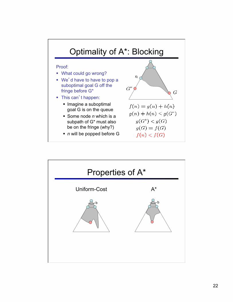
Optimality of A*: Blocking Proof: §  What could go wrong? §  We’d have to have to pop a

suboptimal goal G off the fringe before G*

§  This can’t happen: §  Imagine a suboptimal

goal G is on the queue §  Some node n which is a

subpath of G* must also be on the fringe (why?)

§  n will be popped before G

…

Properties of A*

…b

…b

Uniform-Cost A*

23

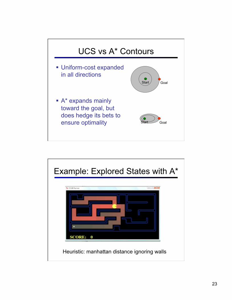
UCS vs A* Contours

§  Uniform-cost expanded in all directions

§  A* expands mainly toward the goal, but does hedge its bets to ensure optimality

Start Goal

Start Goal

Example: Explored States with A*

Heuristic: manhattan distance ignoring walls

24

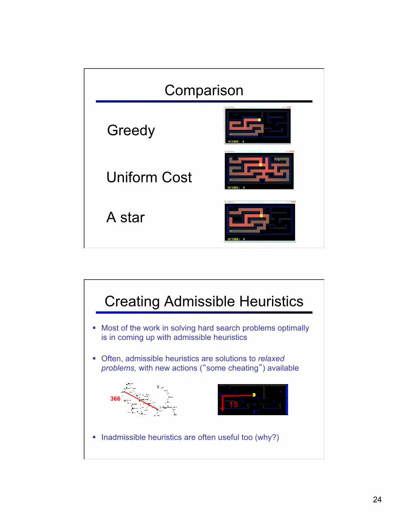
Comparison

Uniform Cost

Greedy

A star

Creating Admissible Heuristics §  Most of the work in solving hard search problems optimally

is in coming up with admissible heuristics

§  Often, admissible heuristics are solutions to relaxed problems, with new actions (“some cheating”) available

§  Inadmissible heuristics are often useful too (why?)

15 366

25

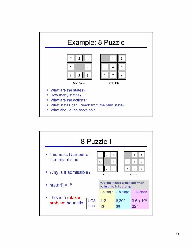
Example: 8 Puzzle

§  What are the states? §  How many states? §  What are the actions? §  What states can I reach from the start state? §  What should the costs be?

8 Puzzle I

§  Heuristic: Number of tiles misplaced

§  Why is it admissible?

§  h(start) =

§  This is a relaxed-problem heuristic

8 Average nodes expanded when optimal path has length…

…4 steps …8 steps …12 steps

UCS 112 6,300 3.6 x 106

TILES 13 39 227

26

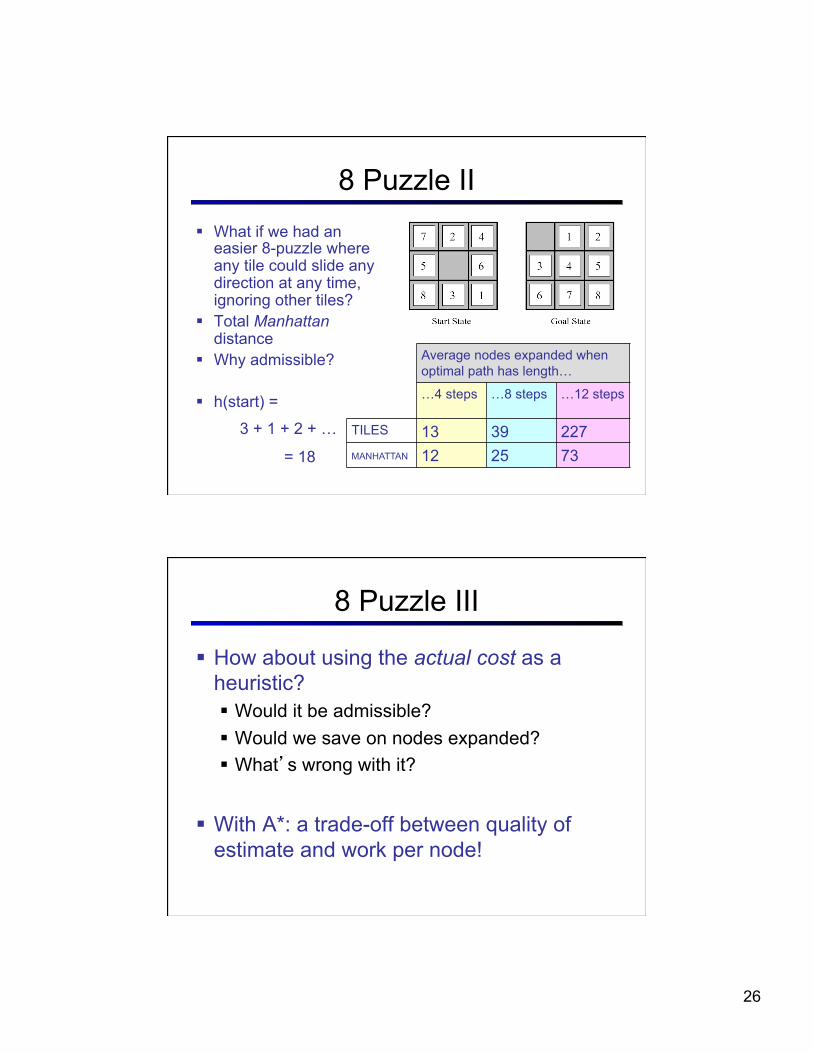
8 Puzzle II §  What if we had an

easier 8-puzzle where any tile could slide any direction at any time, ignoring other tiles?

§  Total Manhattan distance

§  Why admissible?

§  h(start) =

3 + 1 + 2 + …

= 18

Average nodes expanded when optimal path has length…

…4 steps …8 steps …12 steps

TILES 13 39 227

MANHATTAN 12 25 73

8 Puzzle III

§  How about using the actual cost as a heuristic? § Would it be admissible? § Would we save on nodes expanded? § What’s wrong with it?

§  With A*: a trade-off between quality of estimate and work per node!

27

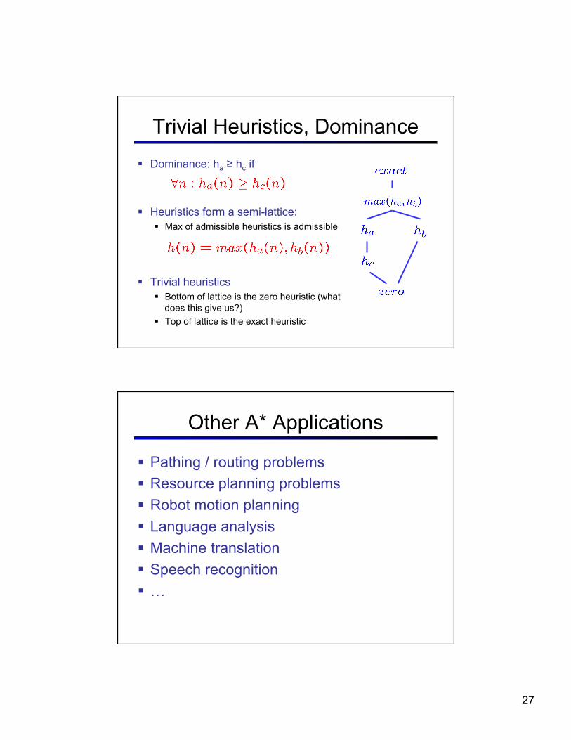
Trivial Heuristics, Dominance §  Dominance: ha ≥ hc if

§  Heuristics form a semi-lattice: §  Max of admissible heuristics is admissible

§  Trivial heuristics §  Bottom of lattice is the zero heuristic (what

does this give us?) §  Top of lattice is the exact heuristic

Other A* Applications

§  Pathing / routing problems §  Resource planning problems §  Robot motion planning §  Language analysis §  Machine translation §  Speech recognition § …

28

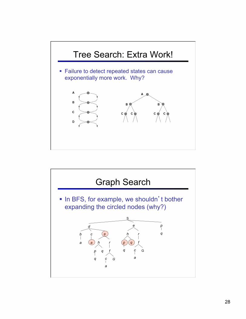
Tree Search: Extra Work!

§  Failure to detect repeated states can cause exponentially more work. Why?

Graph Search

§  In BFS, for example, we shouldn’t bother expanding the circled nodes (why?)

S

a

b

d p

a

c

e

p

h

f

r

q

q c G

a

q e

p

h

f

r

q

q c G

a

29

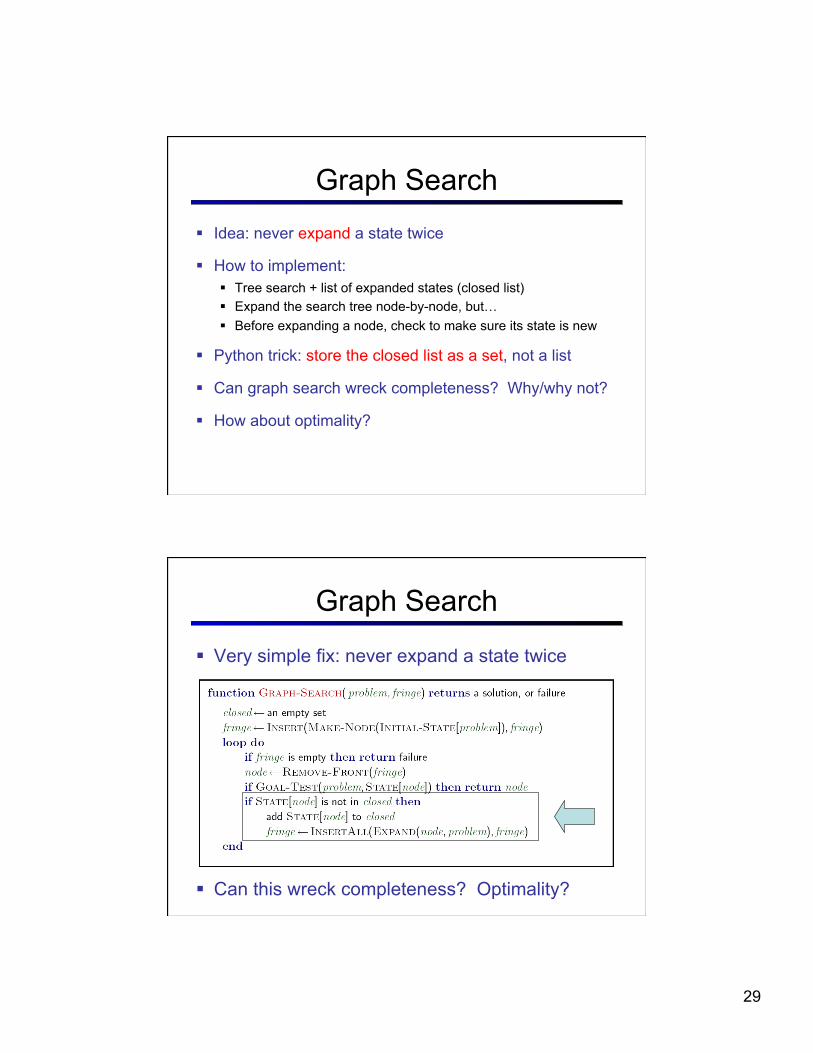
Graph Search §  Idea: never expand a state twice

§  How to implement: §  Tree search + list of expanded states (closed list) §  Expand the search tree node-by-node, but… §  Before expanding a node, check to make sure its state is new

§  Python trick: store the closed list as a set, not a list

§  Can graph search wreck completeness? Why/why not?

§  How about optimality?

Graph Search

§  Very simple fix: never expand a state twice

§  Can this wreck completeness? Optimality?

30

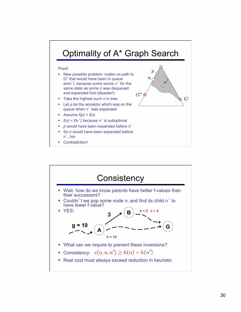
Optimality of A* Graph Search Proof: §  New possible problem: nodes on path to

G* that would have been in queue aren’t, because some worse n’ for the same state as some n was dequeued and expanded first (disaster!)

§  Take the highest such n in tree §  Let p be the ancestor which was on the

queue when n’ was expanded §  Assume f(p) < f(n) §  f(n) < f(n’) because n’ is suboptimal §  p would have been expanded before n’ §  So n would have been expanded before

n’, too §  Contradiction!

Consistency §  Wait, how do we know parents have better f-values than

their successors? §  Couldn’t we pop some node n, and find its child n’ to

have lower f value? §  YES:

§  What can we require to prevent these inversions?

§  Consistency: §  Real cost must always exceed reduction in heuristic

A

B

G

3 h = 0

h = 10

g = 10

h = 8

31

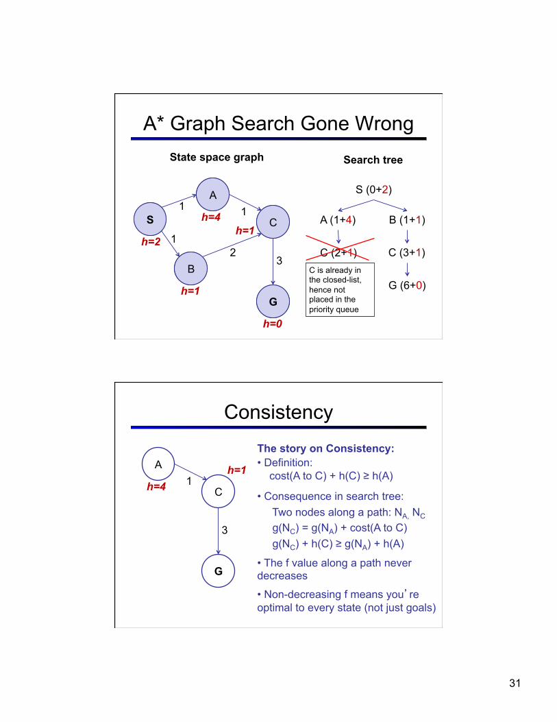
A* Graph Search Gone Wrong

S

A

B

C

G

1

1

1

2 3

h=2

h=1

h=4 h=1

h=0

S (0+2)

A (1+4) B (1+1)

C (2+1) C (3+1)

G (6+0)

S

A

B

C

G

State space graph Search tree

C is already in the closed-list, hence not placed in the priority queue

Consistency

3

A

C

G

h=4 h=1

1

The story on Consistency: •  Definition: cost(A to C) + h(C) ≥ h(A)

•  Consequence in search tree: Two nodes along a path: NA, NC g(NC) = g(NA) + cost(A to C) g(NC) + h(C) ≥ g(NA) + h(A)

•  The f value along a path never decreases

•  Non-decreasing f means you’re optimal to every state (not just goals)

32

Optimality Summary §  Tree search:

§  A* optimal if heuristic is admissible (and non-negative) §  Uniform Cost Search is a special case (h = 0)

§  Graph search: §  A* optimal if heuristic is consistent §  UCS optimal (h = 0 is consistent)

§  Consistency implies admissibility §  Challenge:Try to prove this. §  Hint: try to prove the equivalent statement not admissible implies not

consistent

§  In general, natural admissible heuristics tend to be consistent

§  Remember, costs are always positive in search!

Summary: A*

§  A* uses both backward costs and (estimates of) forward costs

§  A* is optimal with admissible heuristics

§  Heuristic design is key: often use relaxed problems

33

69

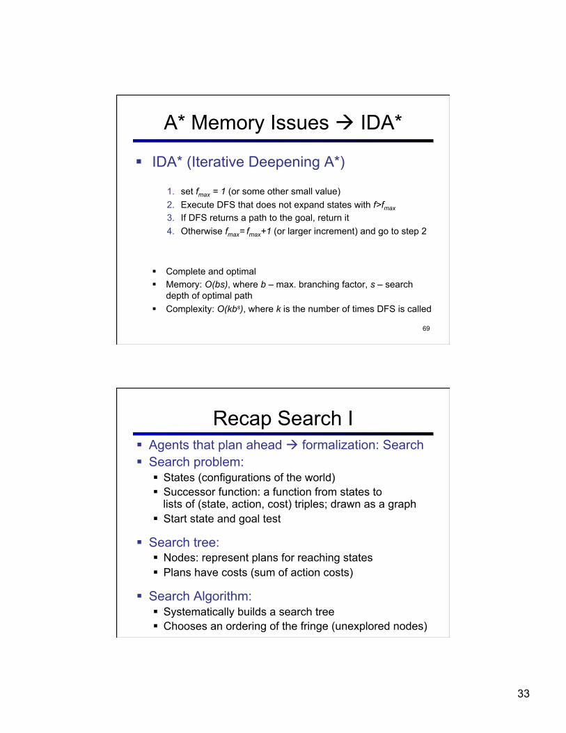
A* Memory Issues à IDA*

§  IDA* (Iterative Deepening A*)

1.  set fmax = 1 (or some other small value) 2.  Execute DFS that does not expand states with f>fmax 3.  If DFS returns a path to the goal, return it 4.  Otherwise fmax= fmax+1 (or larger increment) and go to step 2

§  Complete and optimal §  Memory: O(bs), where b – max. branching factor, s – search

depth of optimal path §  Complexity: O(kbs), where k is the number of times DFS is called

Recap Search I §  Agents that plan ahead à formalization: Search §  Search problem:

§  States (configurations of the world) §  Successor function: a function from states to

lists of (state, action, cost) triples; drawn as a graph §  Start state and goal test

§  Search tree: §  Nodes: represent plans for reaching states §  Plans have costs (sum of action costs)

§  Search Algorithm: §  Systematically builds a search tree §  Chooses an ordering of the fringe (unexplored nodes)

34

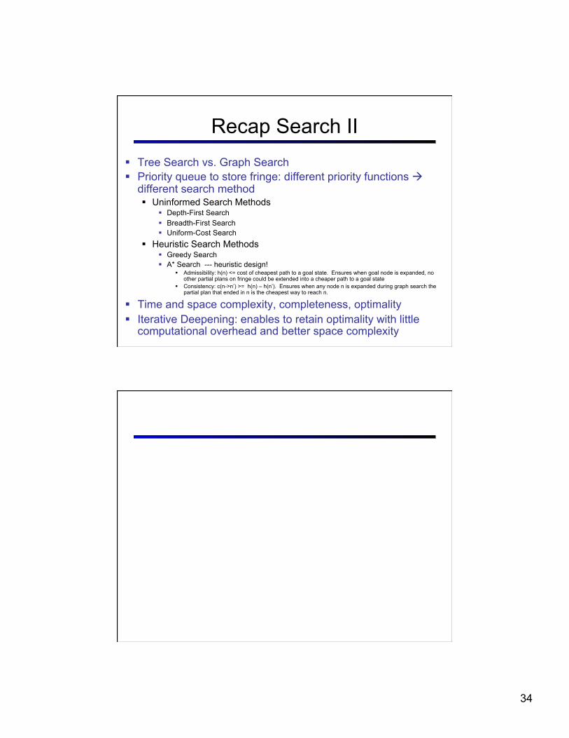
Recap Search II §  Tree Search vs. Graph Search §  Priority queue to store fringe: different priority functions à

different search method §  Uninformed Search Methods

§  Depth-First Search §  Breadth-First Search §  Uniform-Cost Search

§  Heuristic Search Methods §  Greedy Search §  A* Search --- heuristic design!

§  Admissibility: h(n) <= cost of cheapest path to a goal state. Ensures when goal node is expanded, no other partial plans on fringe could be extended into a cheaper path to a goal state

§  Consistency: c(n->n’) >= h(n) – h(n’). Ensures when any node n is expanded during graph search the partial plan that ended in n is the cheapest way to reach n.

§  Time and space complexity, completeness, optimality §  Iterative Deepening: enables to retain optimality with little

computational overhead and better space complexity