Embed Size (px)
Citation preview
CS 4900/5900 Machine Learning:
Razvan C. Bunescu
School of Electrical Engineering and Computer Science
Naïve Bayes
Three Parametric Approaches to Classification
1) Discriminant Functions: construct f : X ® T that directly assigns a vector x to a specific class Ck.– Inference and decision combined into a single learning
problem.– Linear Discriminant: the decision surface is a
hyperplane in X:• Fisher ‘s Linear Discriminant• Perceptron• Support Vector Machines
2
Three Parametric Approaches to Classification
2) Probabilistic Discriminative Models: directly model the posterior class probabilities p(Ck | x).– Inference and decision are separate.– Less data needed to estimate p(Ck | x) than p(x |Ck).– Can accommodate many overlapping features.
• Logistic Regression• Conditional Random Fields
3
Three Parametric Approaches to Classification
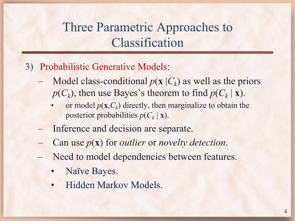
3) Probabilistic Generative Models: – Model class-conditional p(x |Ck) as well as the priors
p(Ck), then use Bayes’s theorem to find p(Ck | x).• or model p(x,Ck) directly, then marginalize to obtain the
posterior probabilities p(Ck | x).
– Inference and decision are separate.– Can use p(x) for outlier or novelty detection.– Need to model dependencies between features.
• Naïve Bayes.• Hidden Markov Models.
4
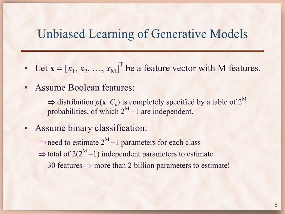
Unbiased Learning of Generative Models
• Let x = [x1, x2, …, xM]T be a feature vector with M features.
• Assume Boolean features:Þ distribution p(x |Ck) is completely specified by a table of 2M
probabilities, of which 2M -1 are independent.
• Assume binary classification:Þneed to estimate 2M -1 parameters for each classÞ total of 2(2M -1) independent parameters to estimate.– 30 features Þ more than 2 billion parameters to estimate!
5
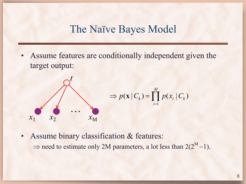
The Naïve Bayes Model
• Assume features are conditionally independent given the target output:
• Assume binary classification & features:Þ need to estimate only 2M parameters, a lot less than 2(2M -1).
6
Õ=
=ÞM
ikik CxpCp
1)|()|(x
…
t
x1 x2 xM
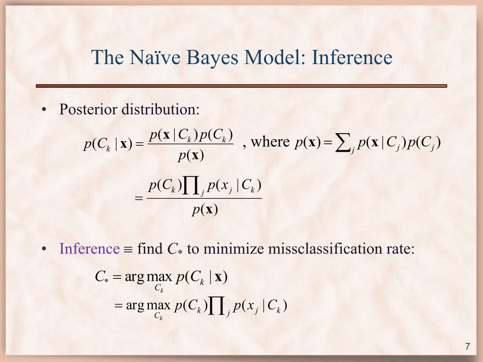
The Naïve Bayes Model: Inference
• Posterior distribution:
• Inference º find C* to minimize missclassification rate:
7
)()()|()|(
xxxp
CpCpCp kkk = å= j jj CpCpp )()|()( xx
)(
)|()(
xp
CxpCpj kjk Õ
=
, where
)|(maxarg* xkCCpC
k
=
Õ=j kjkC
CxpCpk
)|()(maxarg
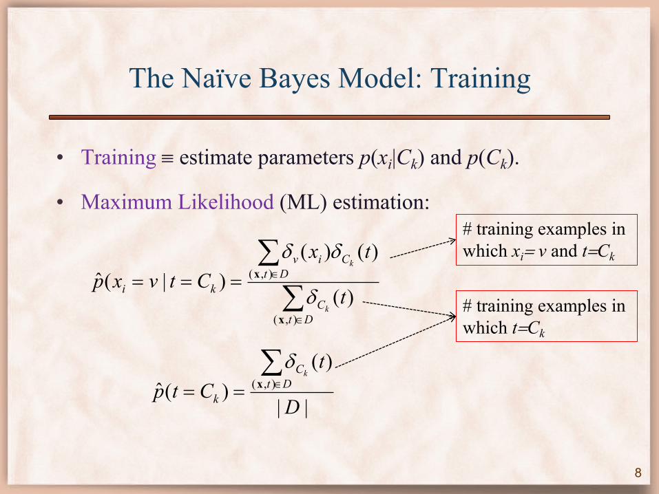
The Naïve Bayes Model: Training
• Training º estimate parameters p(xi|Ck) and p(Ck).
• Maximum Likelihood (ML) estimation:
8
åå
Î
Î===
DtC
DtCiv
ki t
txCtvxp
k
k
),(
),(
)(
)()()|(ˆ
x
x
d
dd
||
)()(ˆ ),(
D
tCtp Dt
C
k
kåÎ== xd
# training examples in which xi= v and t=Ck
# training examples in which t=Ck
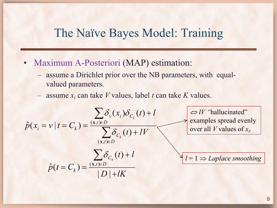
The Naïve Bayes Model: Training
• Maximum A-Posteriori (MAP) estimation:– assume a Dirichlet prior over the NB parameters, with equal-
valued parameters.– assume xi can take V values, label t can take K values.
9
åå
Î
Î
+
+===
DtC
DtCiv
ki lVt
ltxCtvxp
k
k
),(
),(
)(
)()()|(ˆ
x
x
d
dd
lKD
ltCtp Dt
C
k
k
+
+==åÎ
||
)()(ˆ ),(x
d
Û lV “hallucinated” examples spread evenly over all V values of xi.
l = 1 Þ Laplace smoothing
Text Categorization with Naïve Bayes
• Text categorization problems:– Spam filtering.– Targeted advertisement in Gmail.– Classification in multiple categories on news websites.
• Representation as one feature per word:Þ each document is a very high dimensional feature vector.
• Most words are rare:– Zipf’s law and heavy tail distribution.Þ feature vectors are sparse.
10
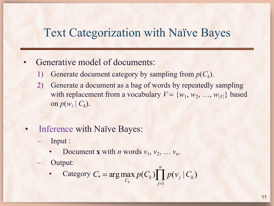
Text Categorization with Naïve Bayes
• Generative model of documents:1) Generate document category by sampling from p(Ck).2) Generate a document as a bag of words by repeatedly sampling
with replacement from a vocabulary V = {w1, w2, …, w|V|} based on p(wi | Ck).
• Inference with Naïve Bayes:– Input :
• Document x with n words v1, v2, … vn.– Output:
• Category
11
Õ=
=n
jkjkCCvpCpC
k 1* )|()(maxarg
Text Categorization with Naïve Bayes
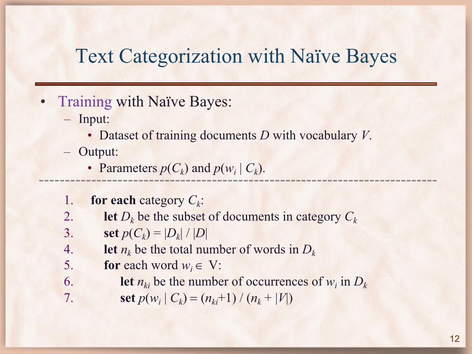
• Training with Naïve Bayes:– Input:
• Dataset of training documents D with vocabulary V.– Output:
• Parameters p(Ck) and p(wi | Ck).
1. for each category Ck:2. let Dk be the subset of documents in category Ck3. set p(Ck) = |Dk| / |D|4. let nk be the total number of words in Dk5. for each word wi Î V:6. let nki be the number of occurrences of wi in Dk7. set p(wi | Ck) = (nki+1) / (nk + |V|)
12
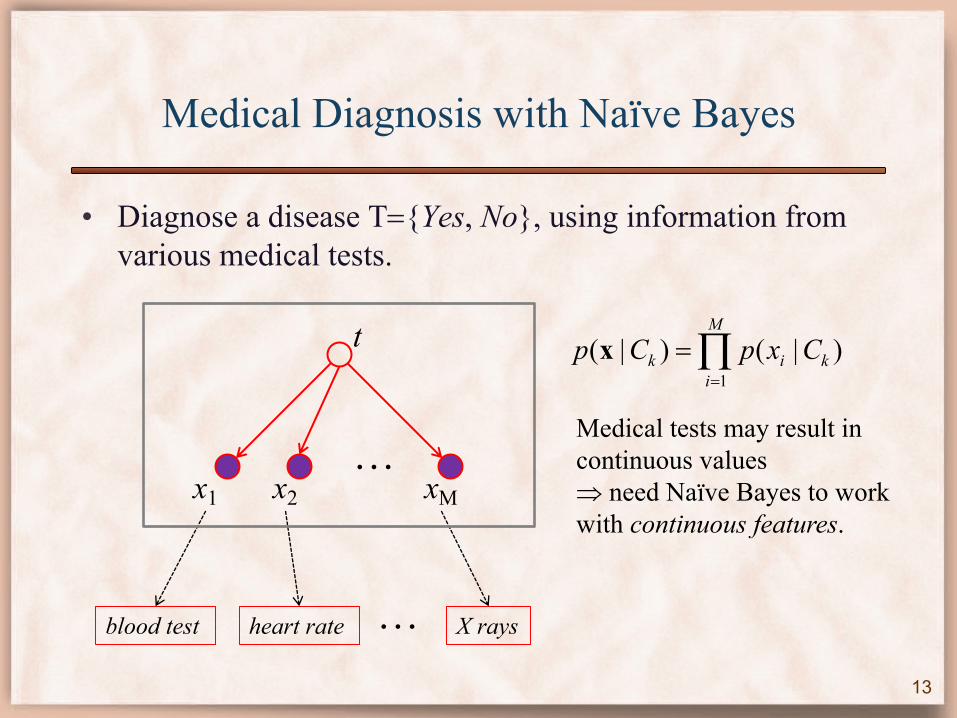
Medical Diagnosis with Naïve Bayes
• Diagnose a disease T={Yes, No}, using information from various medical tests.
13
…
t
x1 x2 xM
blood test X raysheart rate …
Medical tests may result in continuous values Þ need Naïve Bayes to work with continuous features.
Õ=
=M
ikik CxpCp
1)|()|(x
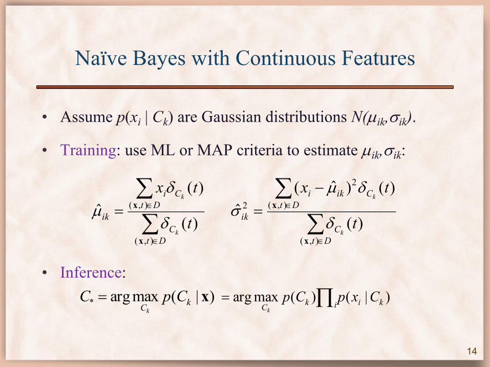
Naïve Bayes with Continuous Features
• Assume p(xi | Ck) are Gaussian distributions N(µik,sik).
• Training: use ML or MAP criteria to estimate µik,sik:
• Inference:
14
åå
Î
Î=
DtC
DtCi
ik t
tx
k
k
),(
),(
)(
)(ˆ
x
x
d
dµ
åå
Î
Î
-=
DtC
DtCiki
ik t
tx
k
k
),(
),(
2
2
)(
)()ˆ(ˆ
x
x
d
dµs
)|(maxarg* xkCCpC
k
= Õ=i kikC
CxpCpk
)|()(maxarg
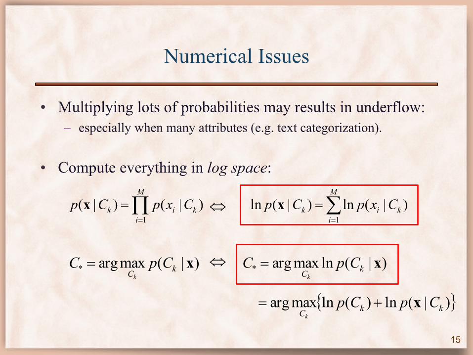
Numerical Issues
• Multiplying lots of probabilities may results in underflow:– especially when many attributes (e.g. text categorization).
• Compute everything in log space:
15
Õ=
=M
ikik CxpCp
1)|()|(x å
=
=M
ikik CxpCp
1)|(ln)|(ln xÛ
)|(maxarg* xkCCpC
k
= Û )|(lnmaxarg* xkCCpC
k
=
{ })|(ln)(lnmaxarg kkCCpCp
k
x+=
Naïve Bayes
• Often has good performance, despite strong independence assumptions:– quite competitive with other classification methods on UCI
datasets.
• It does not produce accurate probability estimates when independence assumptions are violated:– the estimates are still useful for finding max-probability class.
• Does not focus on completely fitting the data Þ resilient to noise.
16
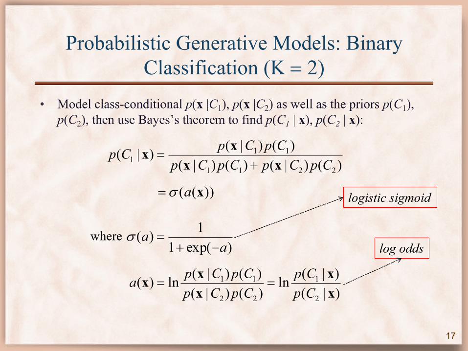
Probabilistic Generative Models: Binary Classification (K = 2)
• Model class-conditional p(x |C1), p(x |C2) as well as the priors p(C1), p(C2), then use Bayes’s theorem to find p(C1 | x), p(C2 | x):
17
)()|()()|()()|()|(
2211
111 CpCpCpCp
CpCpCpxx
xx+
=
))(( xas=
)exp(11)(
aa
-+=s
)|()|(ln
)()|()()|(ln)(
2
1
22
11
xx
xxx
CpCp
CpCpCpCpa ==
logistic sigmoid
log oddswhere
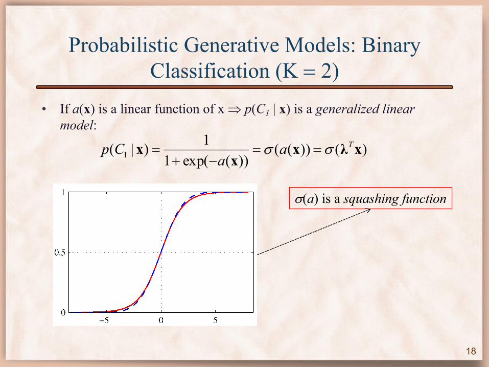
Probabilistic Generative Models: Binary Classification (K = 2)
• If a(x) is a linear function of x Þ p(C1 | x) is a generalized linear model:
18
)())(())(exp(1
1)|( 1 xλxx
x Taa
Cp ss ==-+
=
s(a) is a squashing function
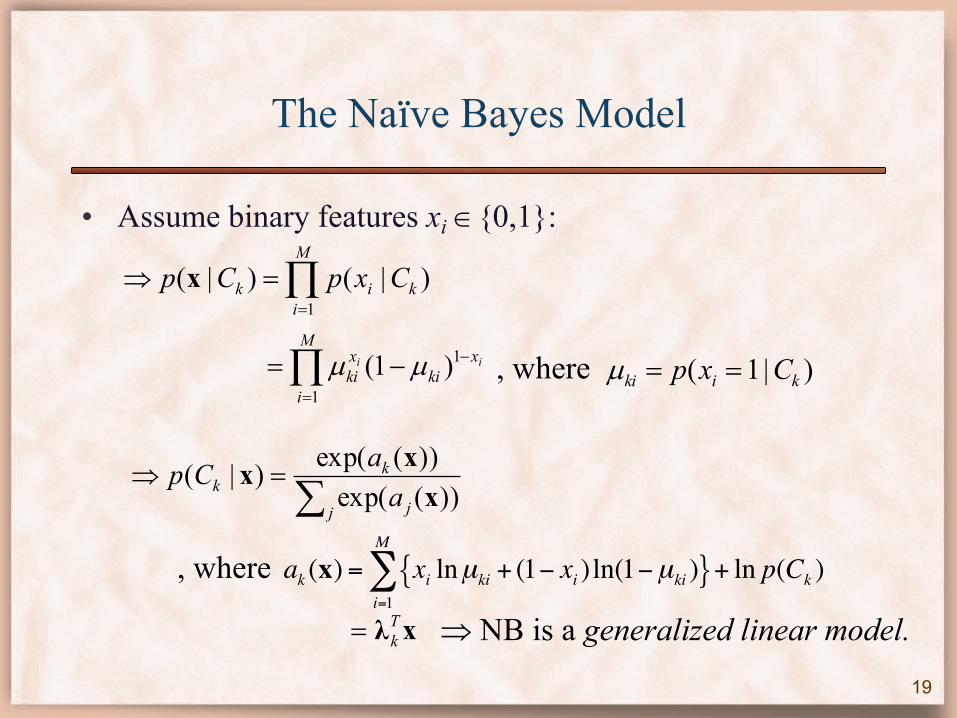
The Naïve Bayes Model
• Assume binary features xi Î{0,1}:
19
Õ=
=ÞM
ikik CxpCp
1)|()|(x
ii xki
M
i
xki
-
=
-=Õ 1
1)1( µµ , where )|1( kiki Cxp ==µ
å=Þ
j j
kk a
aCp))(exp())(exp()|(xxx
, where ak (x) = xi lnµki + (1− xi )ln(1−µki ){ }i=1
M
∑ + ln p(Ck )
xλTk= Þ NB is a generalized linear model.
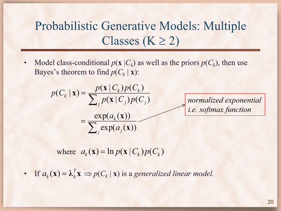
Probabilistic Generative Models: Multiple Classes (K ³ 2)
• Model class-conditional p(x |Ck) as well as the priors p(Ck), then use Bayes’s theorem to find p(Ck | x):
• If Þ p(Ck | x) is a generalized linear model.
20
å=
j jj
kkk CpCp
CpCpCp)()|()()|()|(
xxx
å=
j j
k
aa
))(exp())(exp(xx
normalized exponentiali.e. softmax function
where )()|(ln)( kkk CpCpa xx =
xλx Tkka =)(