CS294-6Reconfigurable Computing

Day 19

October 27, 1998

Multicontext

Today

• Multicontext– Review why– Cost– Packing into contexts– Retiming implications

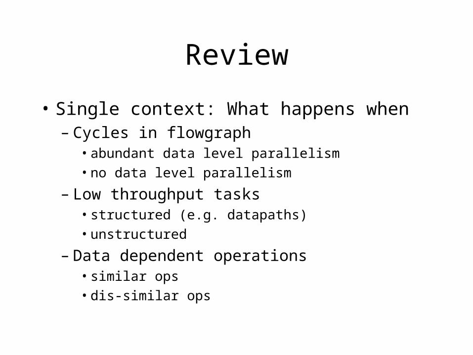
Review

• Single context: What happens when– Cycles in flowgraph

• abundant data level parallelism

• no data level parallelism

– Low throughput tasks• structured (e.g. datapaths)

• unstructured

– Data dependent operations• similar ops

• dis-similar ops

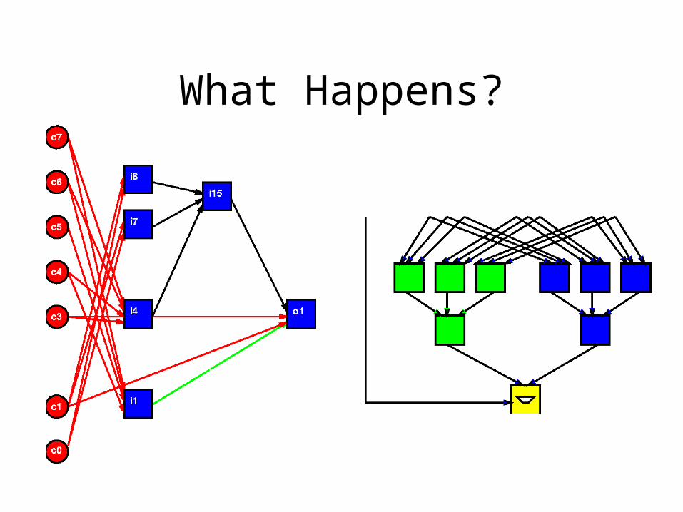
What Happens?

Single Context

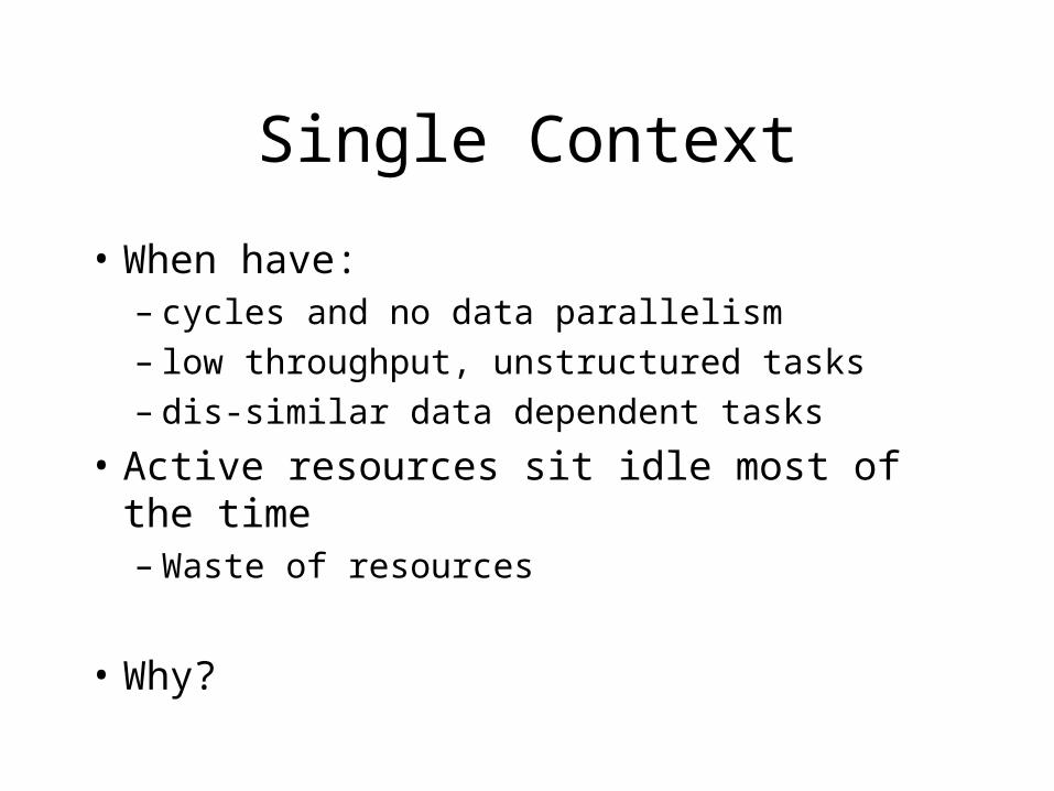
• When have:– cycles and no data parallelism– low throughput, unstructured tasks– dis-similar data dependent tasks

• Active resources sit idle most of the time– Waste of resources

• Why?

Single Context: Why?

• Cannot reuse resources to perform different function, only same

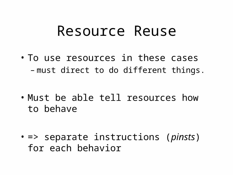
Resource Reuse

• To use resources in these cases– must direct to do different things.

• Must be able tell resources how to behave

• => separate instructions (pinsts) for each behavior

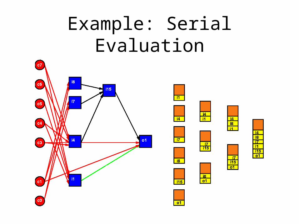
Example: Serial Evaluation

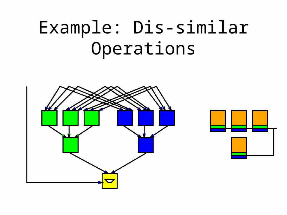
Example: Dis-similar Operations

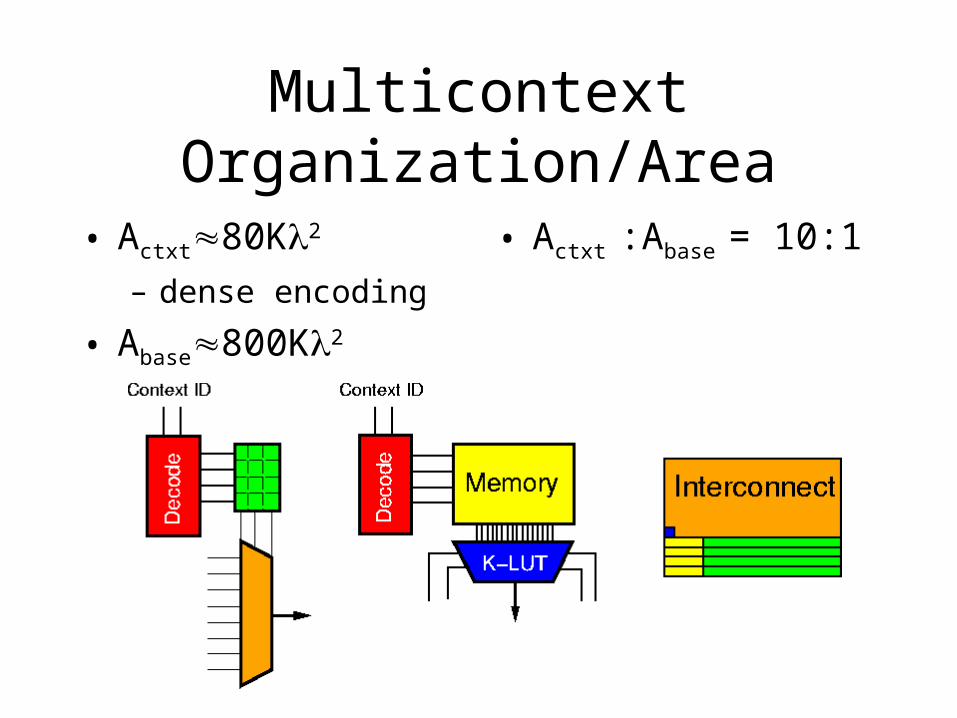
Multicontext Organization/Area

• Actxt80K2

– dense encoding

• Abase800K2

• Actxt :Abase = 10:1

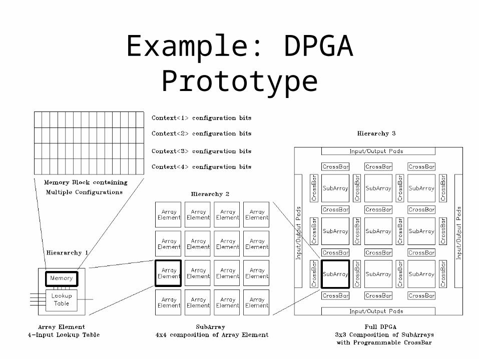
Example: DPGA Prototype

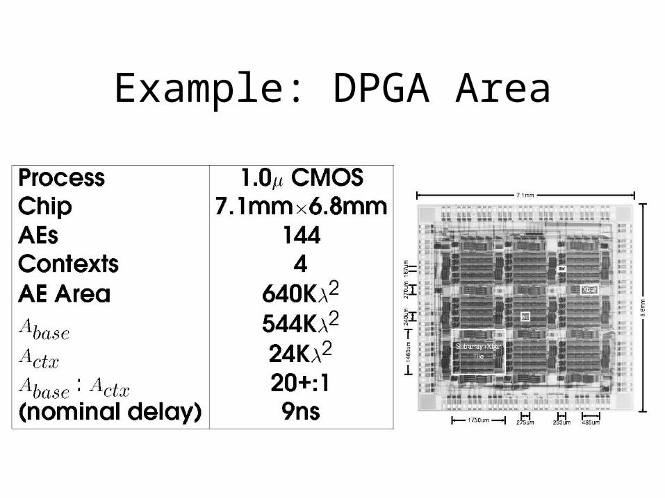
Example: DPGA Area

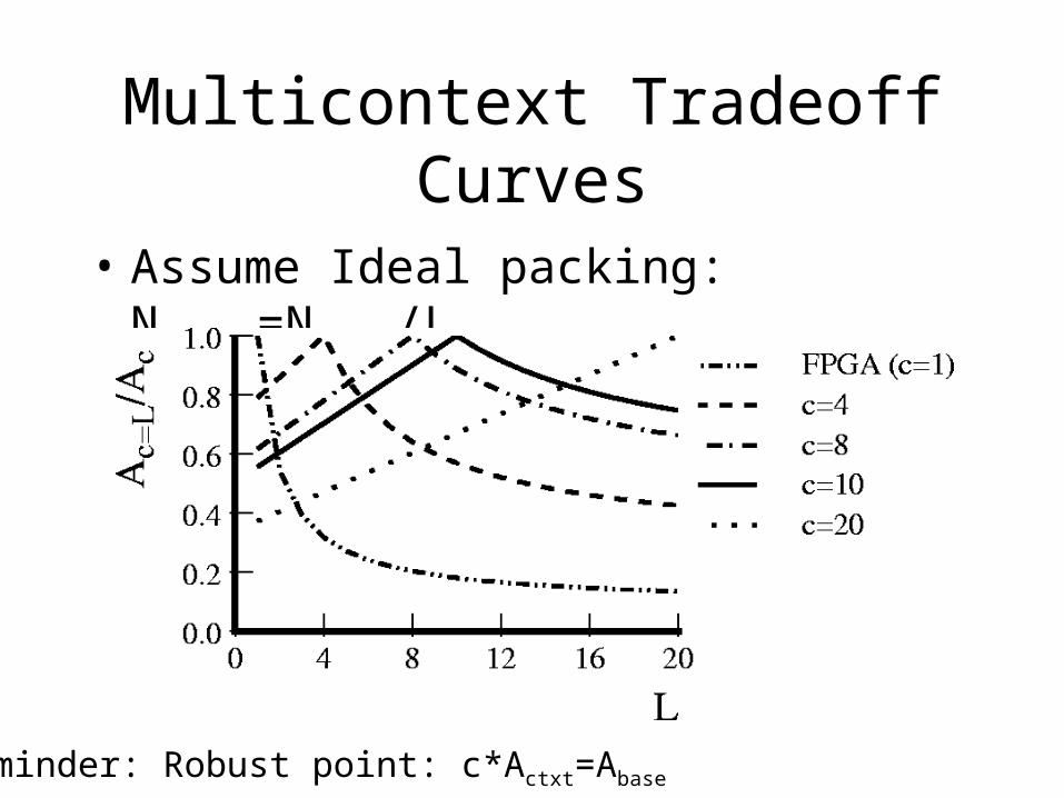
Multicontext Tradeoff Curves

• Assume Ideal packing: Nactive=Ntotal/L

Reminder: Robust point: c*Actxt=Abase

In Practice

• Scheduling Limitations

• Retiming Limitations

Scheduling Limitations

• NA (active)

– size of largest stage

• Precedence: – can evaluate a LUT only after predecessors

have been evaluated– cannot always, completely equalize stage

requirements

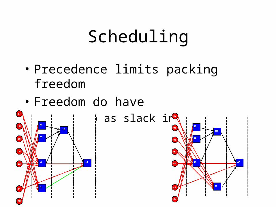
Scheduling

• Precedence limits packing freedom

• Freedom do have – shows up as slack in network

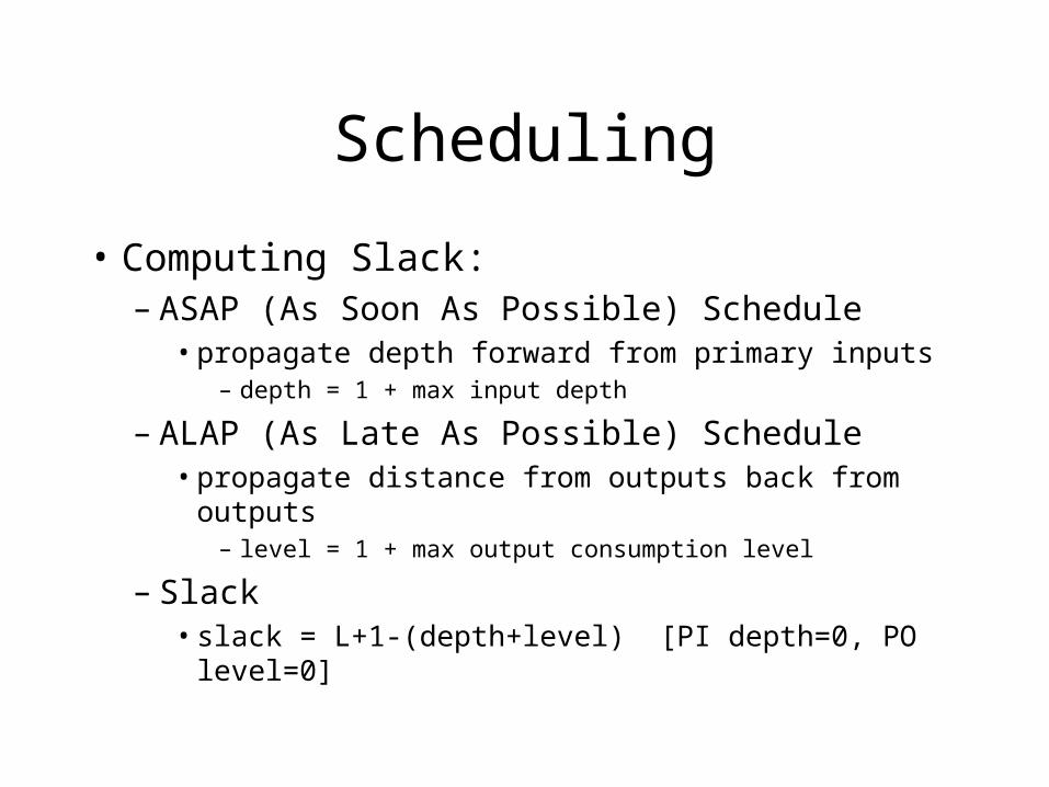
Scheduling

• Computing Slack:– ASAP (As Soon As Possible) Schedule

• propagate depth forward from primary inputs– depth = 1 + max input depth

– ALAP (As Late As Possible) Schedule• propagate distance from outputs back from outputs

– level = 1 + max output consumption level

– Slack• slack = L+1-(depth+level) [PI depth=0, PO level=0]

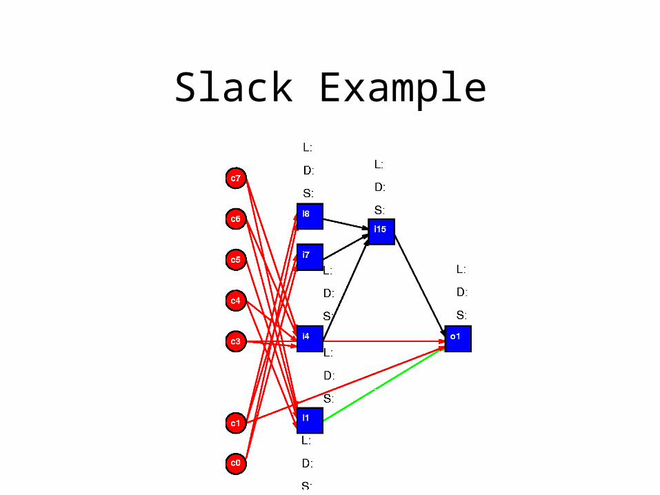
Slack Example

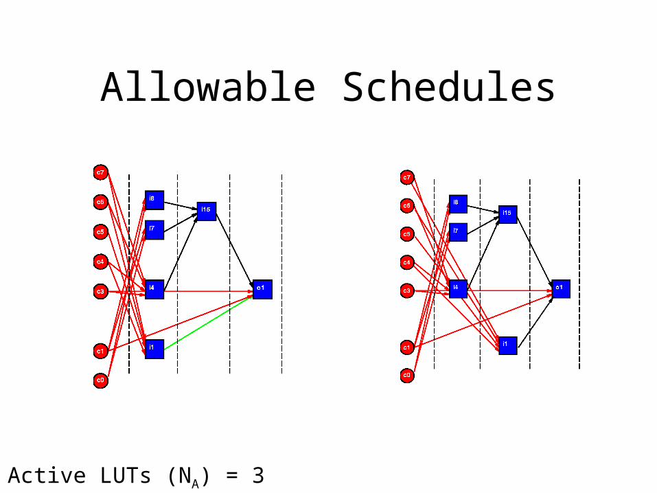
Allowable Schedules

Active LUTs (NA) = 3

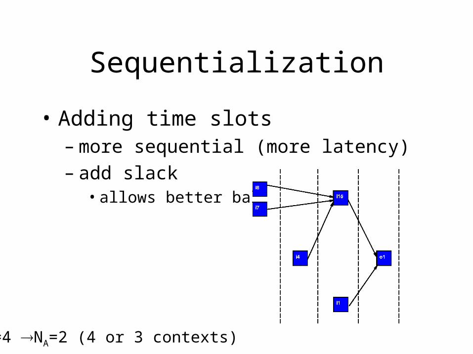
Sequentialization

• Adding time slots – more sequential (more latency)– add slack

• allows better balance

L=4 NA=2 (4 or 3 contexts)

Multicontext Scheduling

• “Retiming” for multicontext– goal: minimize peak resource requirements

• NP-complete

• list schedule, aneal

Multicontext Data Retiming

• How do we accommodate intermediate data?

• Effects?

Signal Retiming

• Non-pipelined – hold value on LUT Output (wire)

• from production through consumption

– Wastes wire and switches by occupying• for entire critical path delay L

• not just for 1/L’th of cycle takes to cross wire segment

– How show up in multicontext?

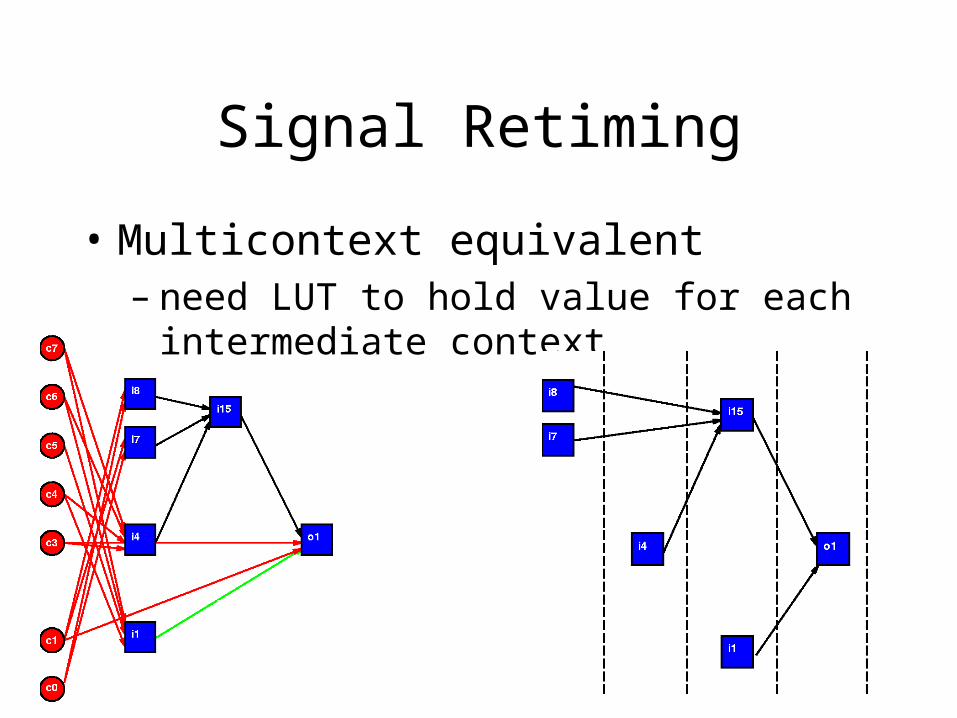
Signal Retiming

• Multicontext equivalent– need LUT to hold value for each intermediate

context

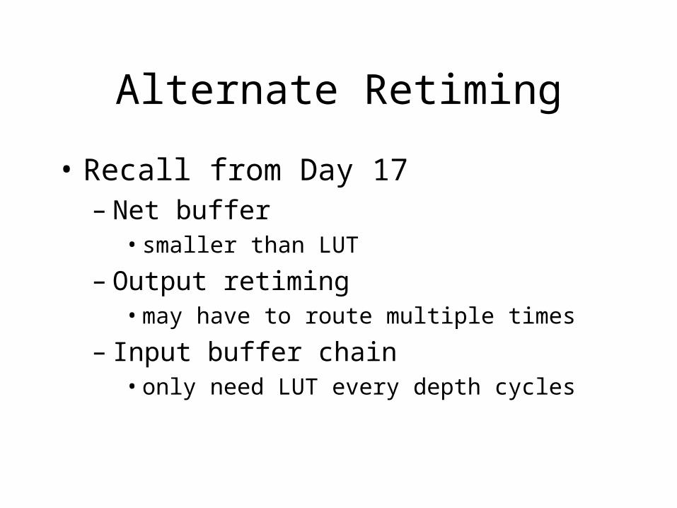
Alternate Retiming

• Recall from Day 17– Net buffer

• smaller than LUT

– Output retiming• may have to route multiple times

– Input buffer chain• only need LUT every depth cycles

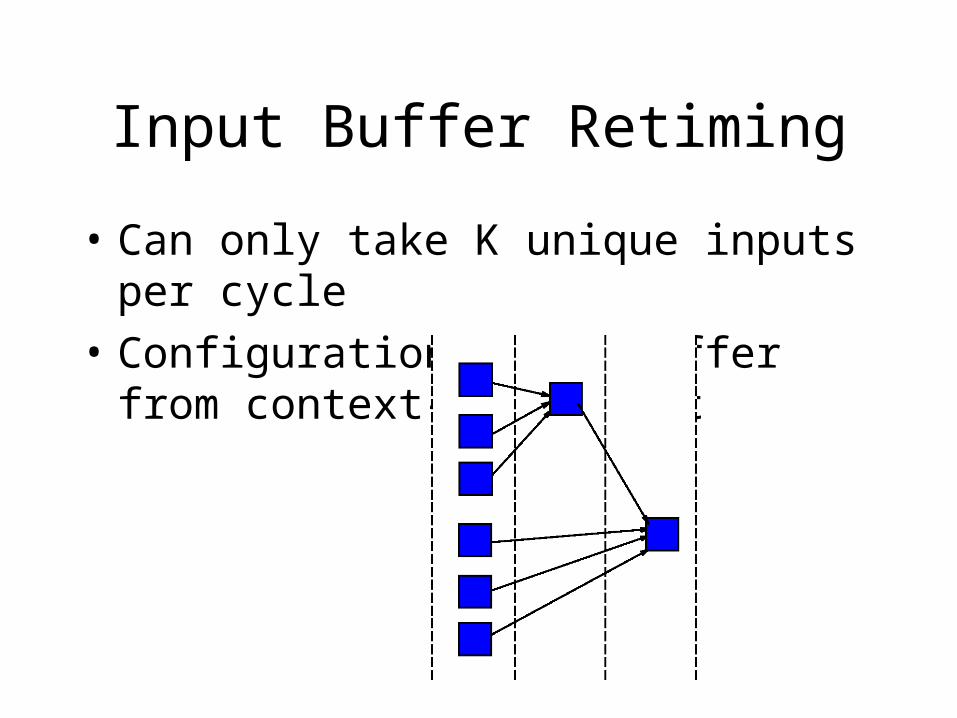
Input Buffer Retiming

• Can only take K unique inputs per cycle

• Configuration depth differ from context-to-context

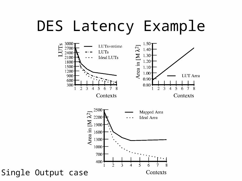
DES Latency Example

Single Output case

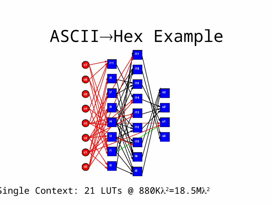
ASCIIHex Example

Single Context: 21 LUTs @ 880K2=18.5M2

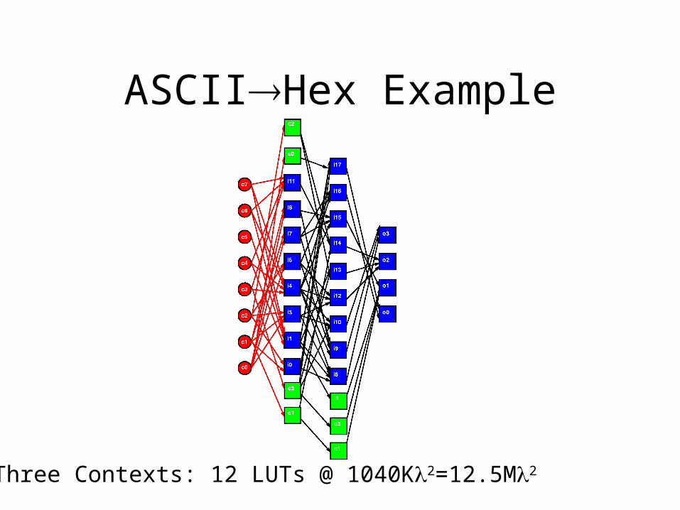
ASCIIHex Example

Three Contexts: 12 LUTs @ 1040K2=12.5M2

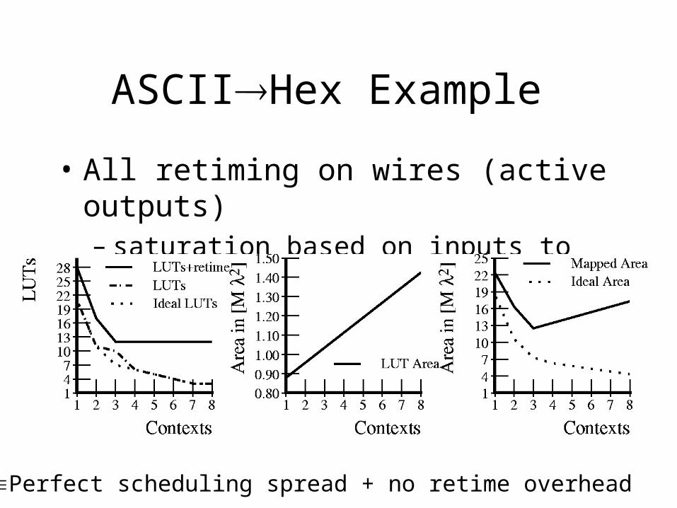
ASCIIHex Example

• All retiming on wires (active outputs)– saturation based on inputs to largest stage

IdealPerfect scheduling spread + no retime overhead

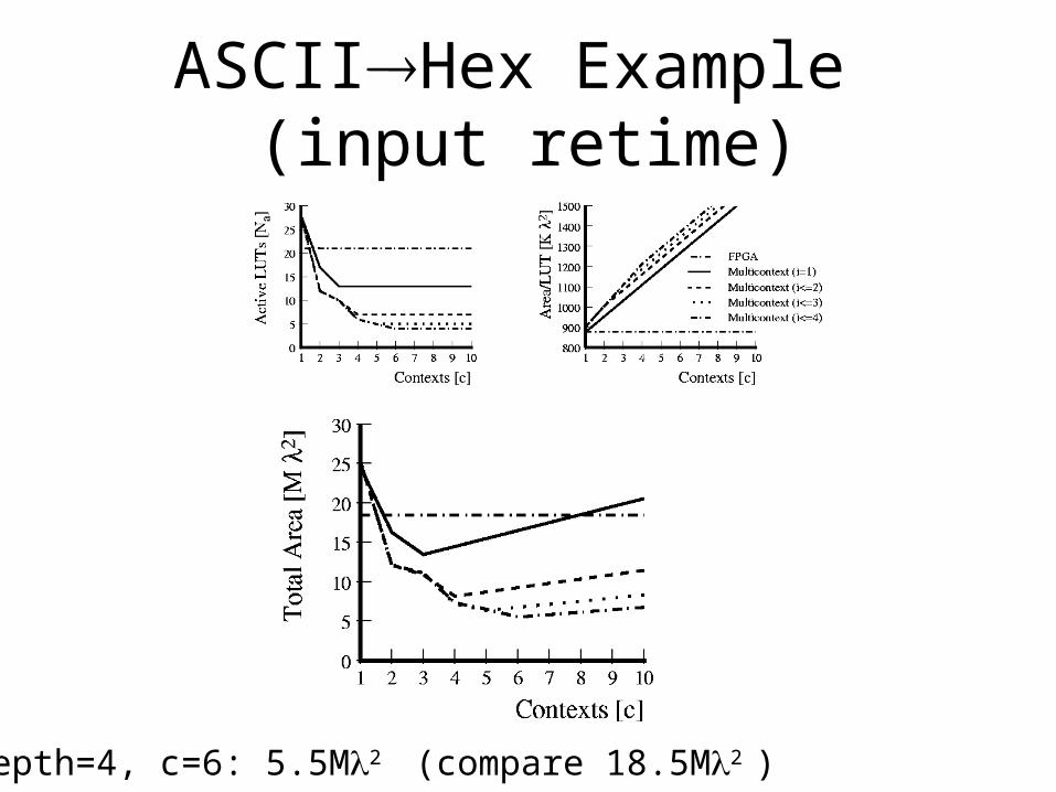
ASCIIHex Example (input retime)

@ depth=4, c=6: 5.5M2 (compare 18.5M2 )

General throughput mapping:

• If only want to achieve limited throughput

• Target produce new result every t cycles

• Spatially pipeline every t stages – cycle = t

• retime to minimize register requirements

• multicontext evaluation w/in a spatial stage– retime (list schedule) to minimize resource

usage

• Map for depth (i) and contexts (c)

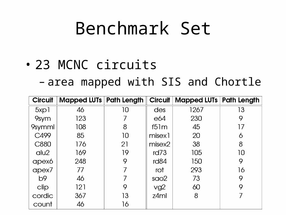
Benchmark Set

• 23 MCNC circuits– area mapped with SIS and Chortle

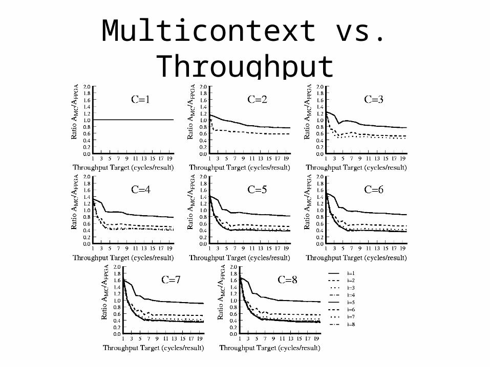
Multicontext vs. Throughput

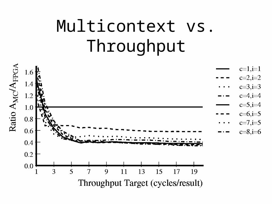
Multicontext vs. Throughput

Summary (1 of 2)

• Several cases cannot profitably reuse same logic at device cycle rate– cycles, no data parallelism

– low throughput, unstructured

– dis-similar data dependent computations

• These cases benefit from more than one instructions/operations per active element

• Actxt<< Aactive makes interesting

– save area by sharing active among instructions

Summary (2 of 2)

• Economical retiming becomes important here to achieve active LUT reduction– one output reg/LUT leads to early saturation

• c=4--8, I=4--6 automatically mapped designs 1/2 to 1/3 single context size

• Most FPGAs typically run in realm where multicontext is smaller– How many for intrinsic reasons?– How many for lack of HSRA-like register/CAD support?