Embed Size (px)
Citation preview
CS38Introduction to Algorithms
Lecture 2
April 3, 2014
April 3, 2014 CS38 Lecture 2 2
Outline
• graph traversals (BFS, DFS)
• connectivity
• topological sort
• strongly connected components
• heaps and heapsort
• greedy algorithms…
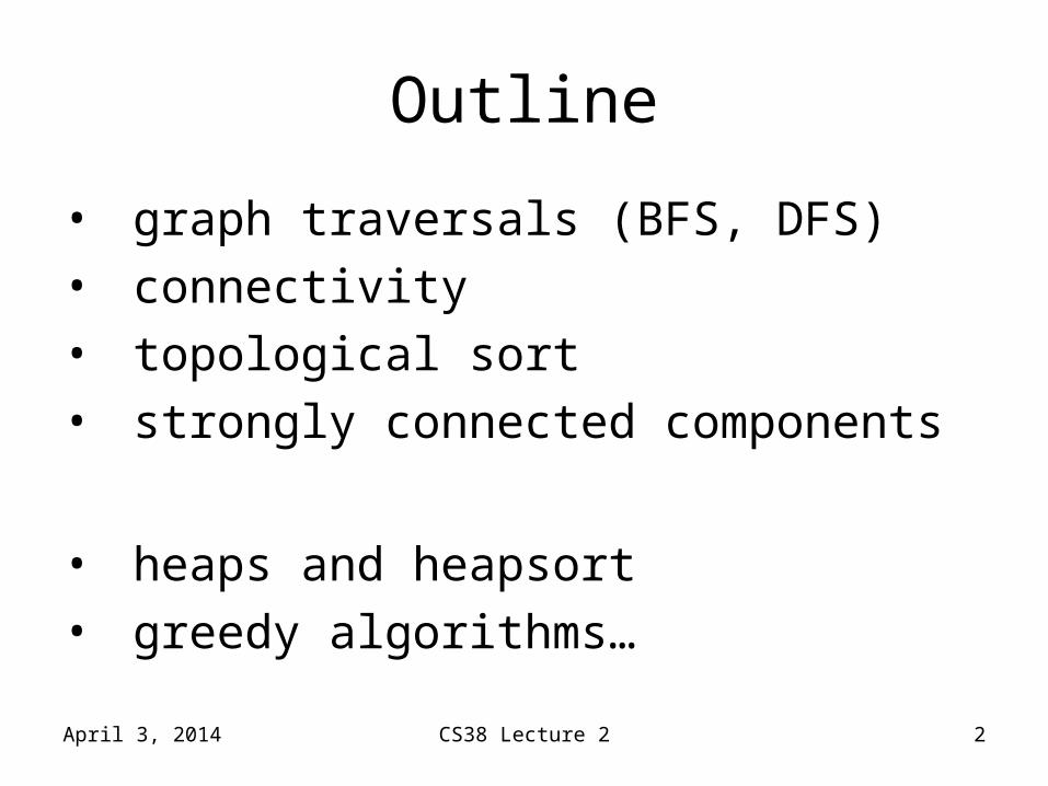
Graphs
• Graph G = (V, E) – directed or undirected– notation: n = |V|, m = |E| (note: m · n2)– adjacency list or adjacency matrix
April 3, 2014 CS38 Lecture 2 3
aa
bb
cc
aa
bb
cc
cc bb
bb
0 1 1
0 0 0
0 1 0
a b ca
b
c
Graphs
• Graphs model many things…– physical networks (e.g. roads)
– communication networks (e.g. internet)
– information networks (e.g. the web)
– social networks (e.g. friends)
– dependency networks (e.g. topics in this course)
… so many fundamental algorithms operate on graphs
April 3, 2014 CS38 Lecture 2 4
Graphs
• Graph terminology:– an undirected graph is connected if there is a
path between each pair of vertices– a tree is a connected, undirected graph with no
cycles; a forest is a collection of disjoint trees– a directed graph is strongly connected if there
is a path from x to y and from y to x, 8 x,y2V
– a DAG is a Directed Acyclic Graph
April 3, 2014 CS38 Lecture 2 5
Graph traversals
• Graph traversal algorithm: visit some or all of the nodes in a graph, labeling them with useful information– breadth-first: useful for undirected, yields
connectivity and shortest-paths information– depth-first: useful for directed, yields
numbering used for• topological sort• strongly-connected component decomposition
April 3, 2014 CS38 Lecture 2 6
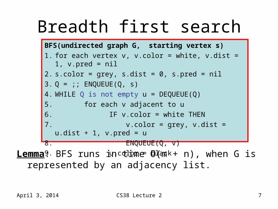
Breadth first searchBFS(undirected graph G, starting vertex s)
1. for each vertex v, v.color = white, v.dist = 1, v.pred = nil
2. s.color = grey, s.dist = 0, s.pred = nil
3. Q = ;; ENQUEUE(Q, s)
4. WHILE Q is not empty u = DEQUEUE(Q)
5. for each v adjacent to u
6. IF v.color = white THEN
7. v.color = grey, v.dist = u.dist + 1, v.pred = u
8. ENQUEUE(Q, v)
9. u.color = black
Lemma: BFS runs in time O(m + n), when G is represented by an adjacency list.
April 3, 2014 7CS38 Lecture 2
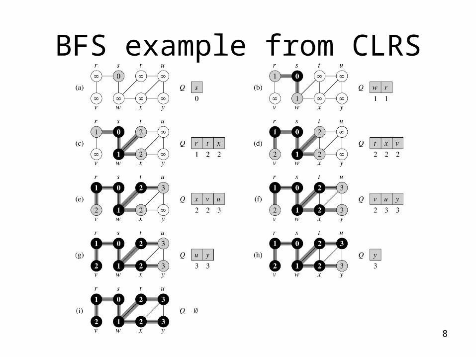
BFS example from CLRS
8
s
Breadth first search
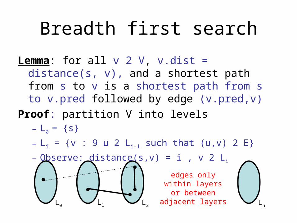
Lemma: for all v 2 V, v.dist = distance(s, v), and a shortest path from s to v is a shortest path from s to v.pred followed by edge (v.pred,v)
Proof: partition V into levels– L0 = {s}
– Li = {v : 9 u 2 Li-1 such that (u,v) 2 E}
– Observe: distance(s,v) = i , v 2 Li
L0 L1 L2 Ln
edges only within layers or between
adjacent layers
Breadth first search
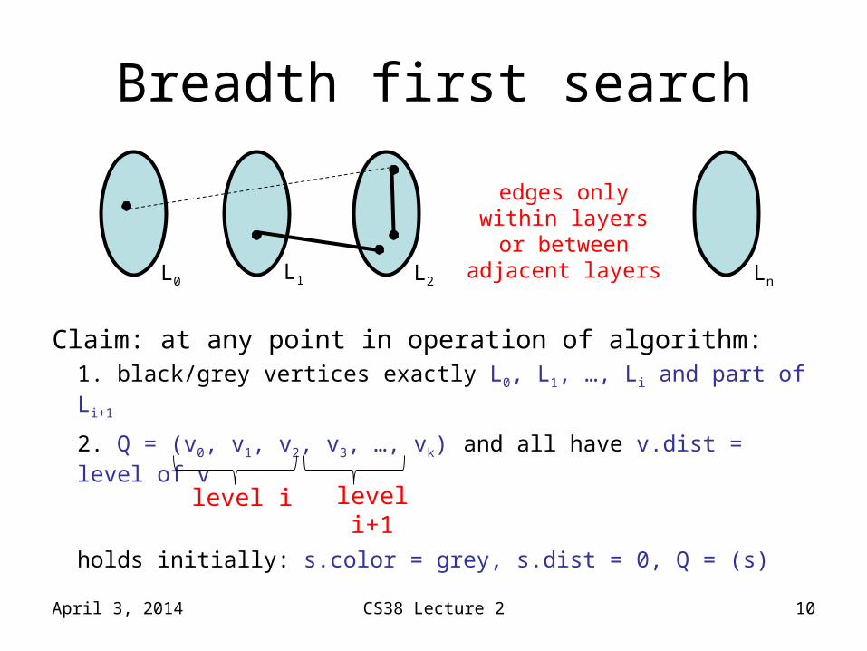
Claim: at any point in operation of algorithm:1. black/grey vertices exactly L0, L1, …, Li and part of Li+1
2. Q = (v0, v1, v2, v3, …, vk) and all have v.dist = level of v
holds initially: s.color = grey, s.dist = 0, Q = (s)
April 3, 2014 CS38 Lecture 2 10
s
L0 L1 L2 Ln
edges only within layers or between
adjacent layers
level i level i+1
Breadth first search
Claim: at any point in operation of algorithm:1. black/grey vertices exactly L0, L1, …, Li and part of Li+1
2. Q = (v0, v1, v2, v3, …, vk) and all have v.dist = level of v
1 step: dequeue v0; add white nbrs of v0 w/ dist = v0.dist + 1
April 3, 2014 CS38 Lecture 2 11
s
L0 L1 L2 Ln
edges only within layers or between
adjacent layers
level i level i+1) level ¸ i+1
) level · i+1
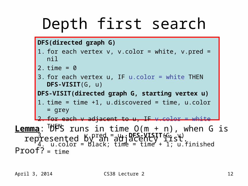
Depth first search
Lemma: DFS runs in time O(m + n), when G is represented by an adjacency list.
Proof?
DFS(directed graph G)
1. for each vertex v, v.color = white, v.pred = nil
2. time = 0
3. for each vertex u, IF u.color = white THEN DFS-VISIT(G, u)
DFS-VISIT(directed graph G, starting vertex u)
1. time = time +1, u.discovered = time, u.color = grey
2. for each v adjacent to u, IF v.color = white THEN
3. v.pred = u, DFS-VISIT(G, v)
4. u.color = black; time = time + 1; u.finished = time
April 3, 2014 12CS38 Lecture 2
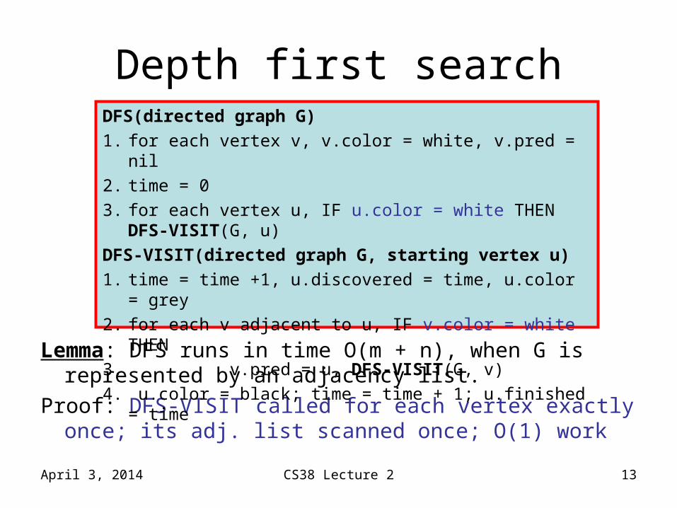
Depth first search
Lemma: DFS runs in time O(m + n), when G is represented by an adjacency list.
Proof: DFS-VISIT called for each vertex exactly once; its adj. list scanned once; O(1) work
DFS(directed graph G)
1. for each vertex v, v.color = white, v.pred = nil
2. time = 0
3. for each vertex u, IF u.color = white THEN DFS-VISIT(G, u)
DFS-VISIT(directed graph G, starting vertex u)
1. time = time +1, u.discovered = time, u.color = grey
2. for each v adjacent to u, IF v.color = white THEN
3. v.pred = u, DFS-VISIT(G, v)
4. u.color = black; time = time + 1; u.finished = time
April 3, 2014 13CS38 Lecture 2
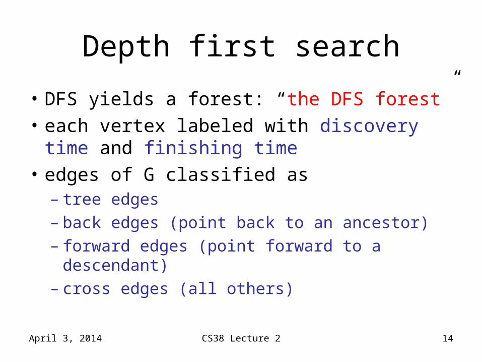
Depth first search
• DFS yields a forest: “the DFS forest”
• each vertex labeled with discovery time and finishing time
• edges of G classified as– tree edges– back edges (point back to an ancestor)– forward edges (point forward to a descendant)– cross edges (all others)
April 3, 2014 CS38 Lecture 2 14

DFS example from CLRS
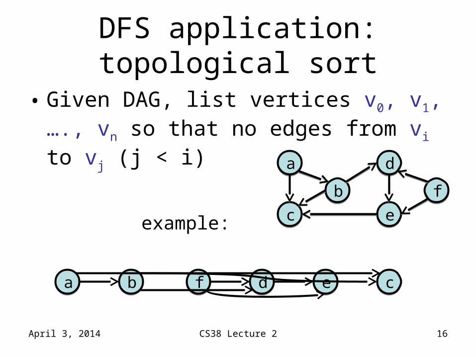
DFS application: topological sort
• Given DAG, list vertices v0, v1, …., vn so that no edges from vi to vj (j < i)
example:
April 3, 2014 CS38 Lecture 2 16
aa
bb
cc
dd
ff
ee
cceeddffbbaa
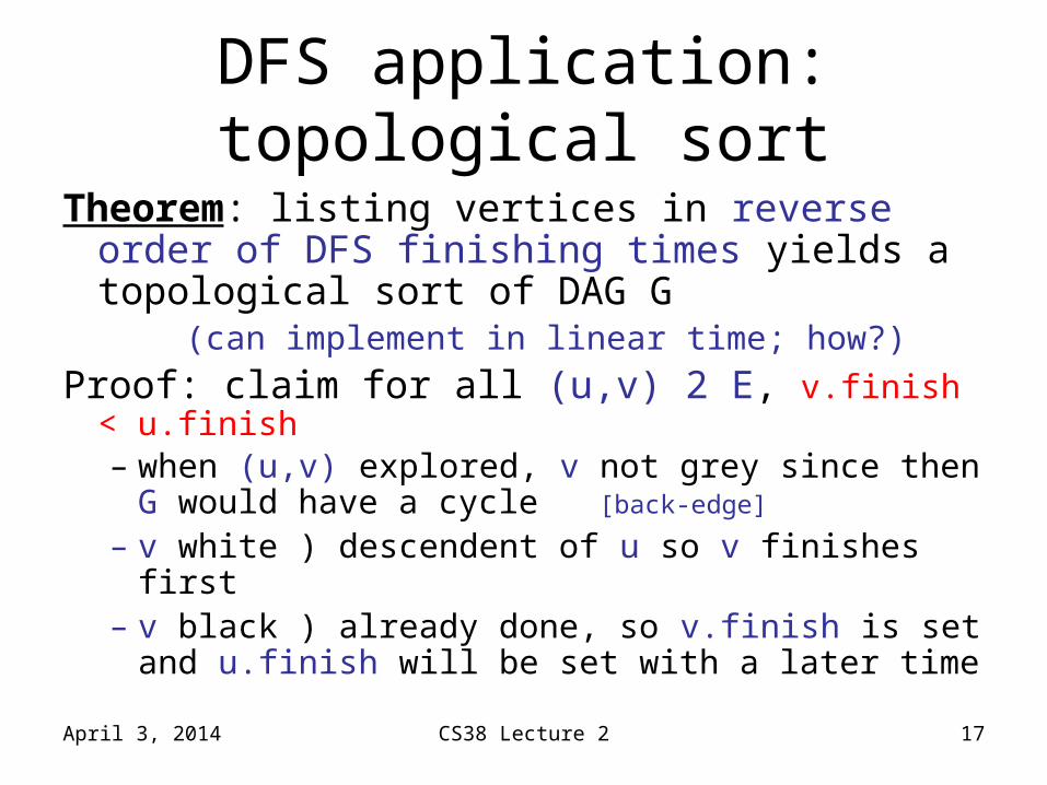
DFS application: topological sort
Theorem: listing vertices in reverse order of DFS finishing times yields a topological sort of DAG G
(can implement in linear time; how?)
Proof: claim for all (u,v) 2 E, v.finish < u.finish– when (u,v) explored, v not grey since then G
would have a cycle [back-edge]
– v white ) descendent of u so v finishes first– v black ) already done, so v.finish is set and
u.finish will be set with a later time
April 3, 2014 CS38 Lecture 2 17
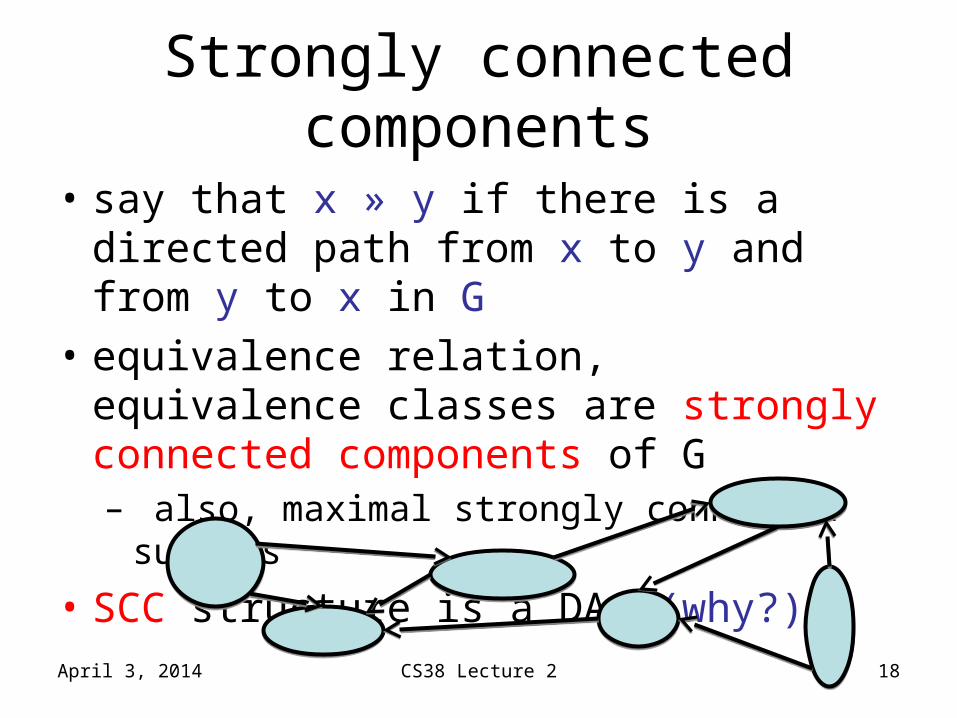
Strongly connected components
• say that x » y if there is a directed path from x to y and from y to x in G
• equivalence relation, equivalence classes are strongly connected components of G– also, maximal strongly connected subsets
• SCC structure is a DAG (why?)
April 3, 2014 CS38 Lecture 2 18
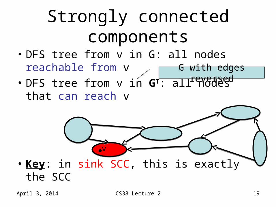
Strongly connected components
• DFS tree from v in G: all nodes reachable from v
• DFS tree from v in GT: all nodes that can reach v
• Key: in sink SCC, this is exactly the SCC
April 3, 2014 CS38 Lecture 2 19
G with edges reversedG with edges reversed
v
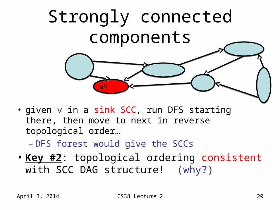
Strongly connected components
• given v in a sink SCC, run DFS starting there, then move to next in reverse topological order…– DFS forest would give the SCCs
• Key #2: topological ordering consistent with SCC DAG structure! (why?)
April 3, 2014 CS38 Lecture 2 20
v
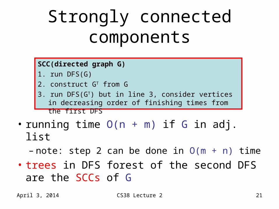
Strongly connected components
• running time O(n + m) if G in adj. list – note: step 2 can be done in O(m + n) time
• trees in DFS forest of the second DFS are the SCCs of G
April 3, 2014 CS38 Lecture 2 21
SCC(directed graph G)
1. run DFS(G)
2. construct GT from G
3. run DFS(GT) but in line 3, consider vertices in decreasing order of finishing times from the first DFS
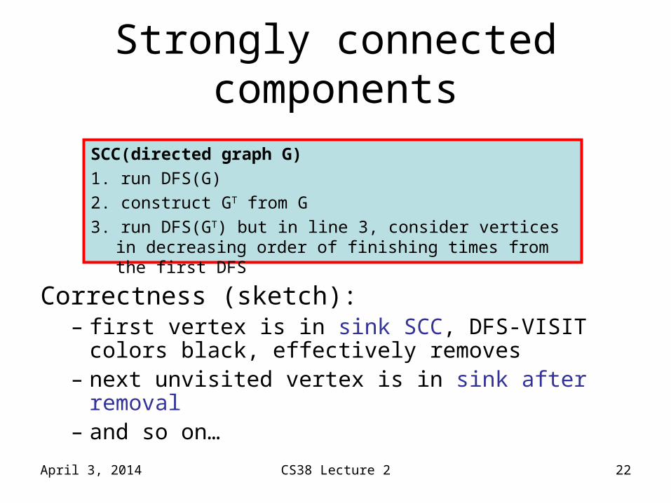
Strongly connected components
Correctness (sketch):– first vertex is in sink SCC, DFS-VISIT colors
black, effectively removes– next unvisited vertex is in sink after removal– and so on…
April 3, 2014 CS38 Lecture 2 22
SCC(directed graph G)
1. run DFS(G)
2. construct GT from G
3. run DFS(GT) but in line 3, consider vertices in decreasing order of finishing times from the first DFS
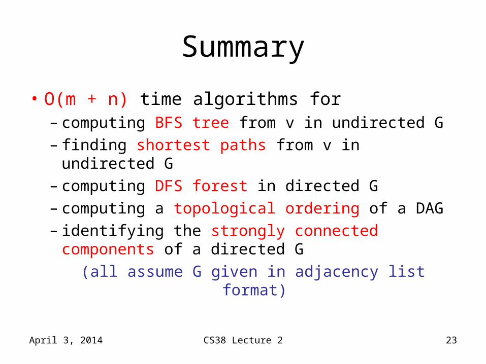
Summary
• O(m + n) time algorithms for– computing BFS tree from v in undirected G– finding shortest paths from v in undirected G– computing DFS forest in directed G– computing a topological ordering of a DAG– identifying the strongly connected
components of a directed G
(all assume G given in adjacency list format)
April 3, 2014 CS38 Lecture 2 23
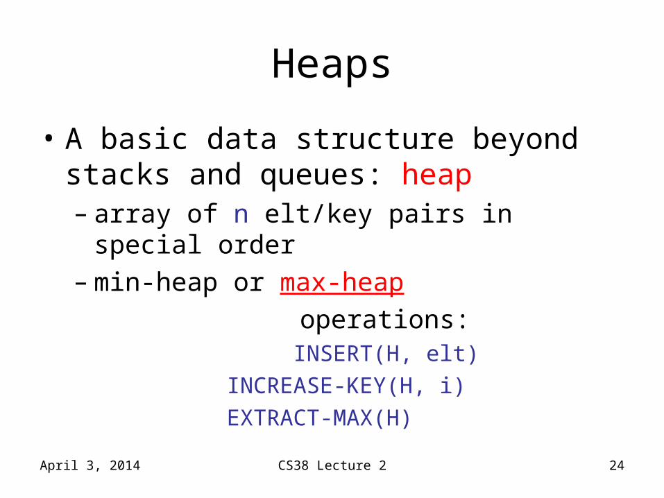
Heaps
• A basic data structure beyond stacks and queues: heap– array of n elt/key pairs in special order– min-heap or max-heap
operations: INSERT(H, elt)
INCREASE-KEY(H, i)
EXTRACT-MAX(H)
April 3, 2014 CS38 Lecture 2 24
Heaps
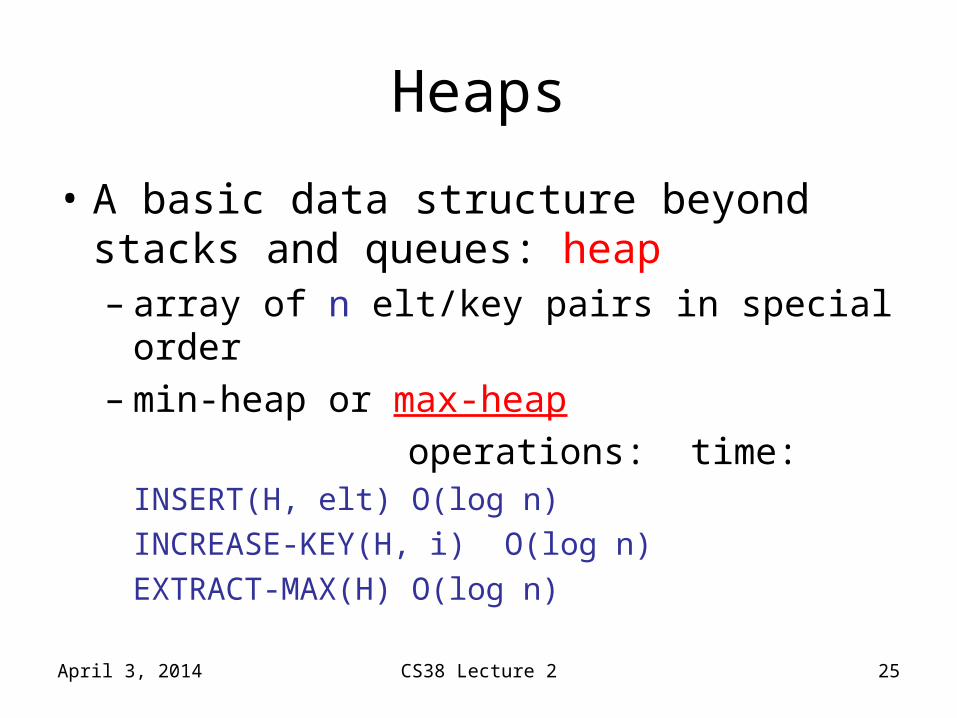
• A basic data structure beyond stacks and queues: heap– array of n elt/key pairs in special order– min-heap or max-heap
operations: time:INSERT(H, elt) O(log n)
INCREASE-KEY(H, i) O(log n)
EXTRACT-MAX(H) O(log n)
April 3, 2014 CS38 Lecture 2 25
Heaps
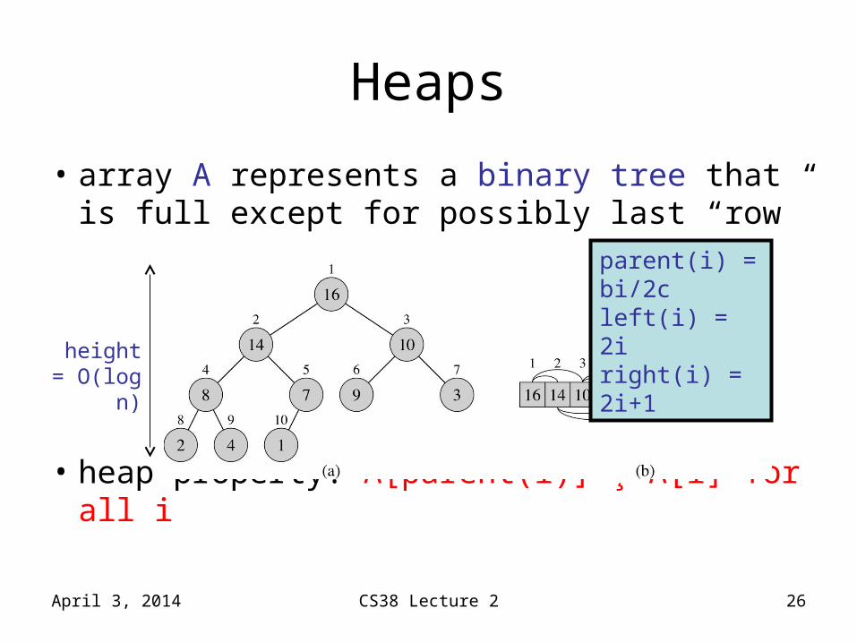
• array A represents a binary tree that is full except for possibly last “row”
• heap property: A[parent(i)] ¸ A[i] for all i
April 3, 2014 CS38 Lecture 2 26
parent(i) = bi/2cleft(i) = 2iright(i) = 2i+1height =
O(log n)
Heaps
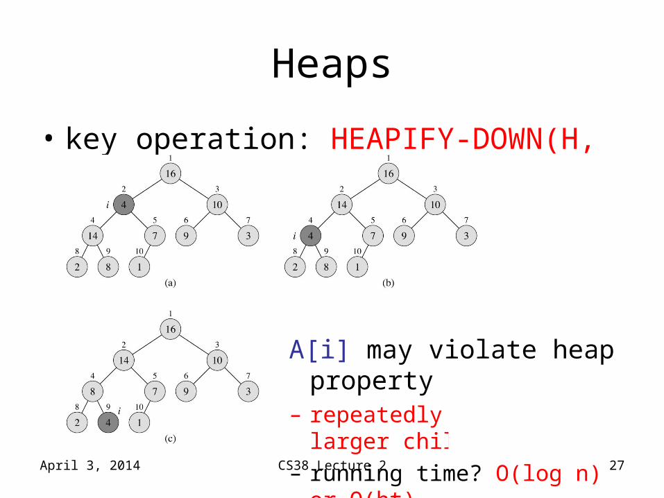
• key operation: HEAPIFY-DOWN(H, i)
April 3, 2014 CS38 Lecture 2 27
A[i] may violate heap property – repeatedly swap with larger child– running time? O(log n) or O(ht)
Heaps
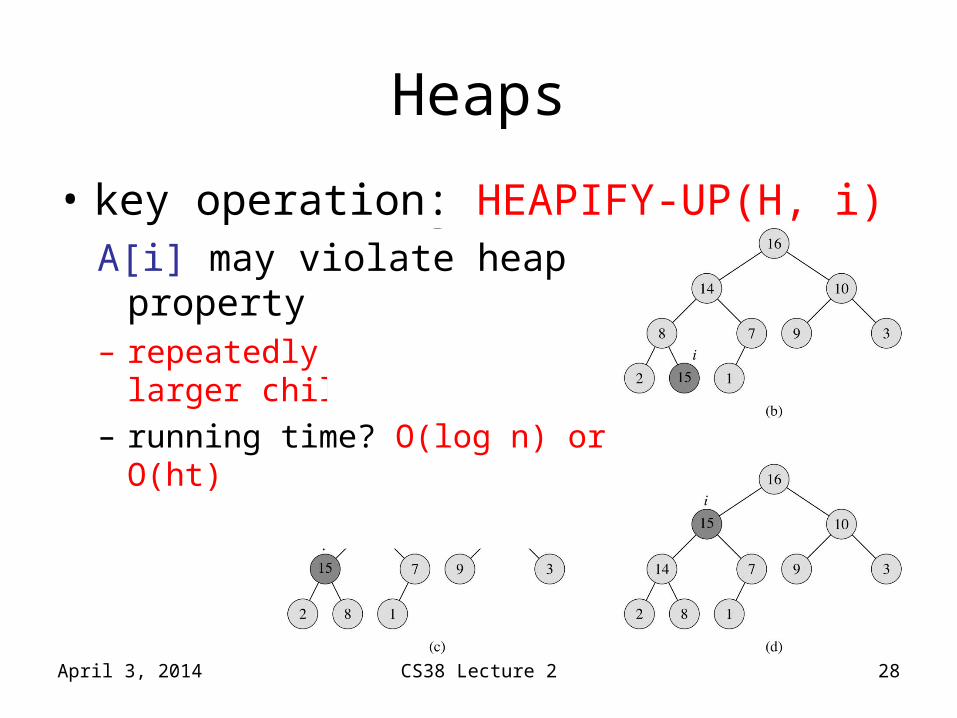
• key operation: HEAPIFY-UP(H, i)
April 3, 2014 CS38 Lecture 2 28
A[i] may violate heap property – repeatedly swap with larger child– running time? O(log n) or O(ht)
Heaps
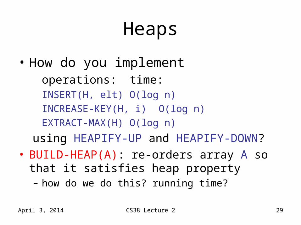
• How do you implementoperations: time:INSERT(H, elt) O(log n)
INCREASE-KEY(H, i) O(log n)
EXTRACT-MAX(H) O(log n)
using HEAPIFY-UP and HEAPIFY-DOWN?• BUILD-HEAP(A): re-orders array A so that it
satisfies heap property– how do we do this? running time?
April 3, 2014 CS38 Lecture 2 29
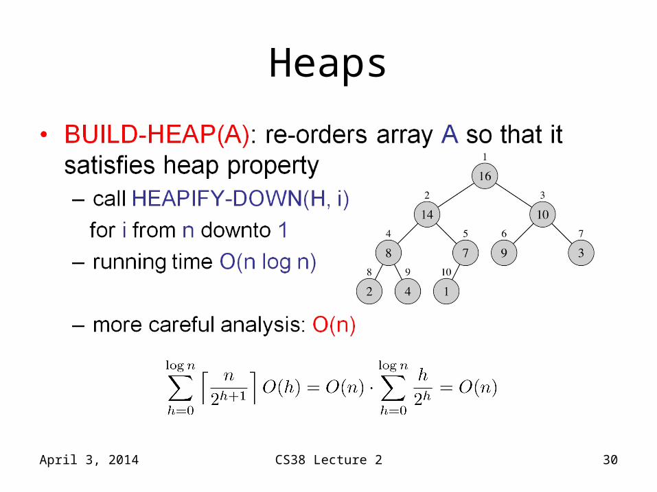
Heaps
April 3, 2014 CS38 Lecture 2 30
Heaps
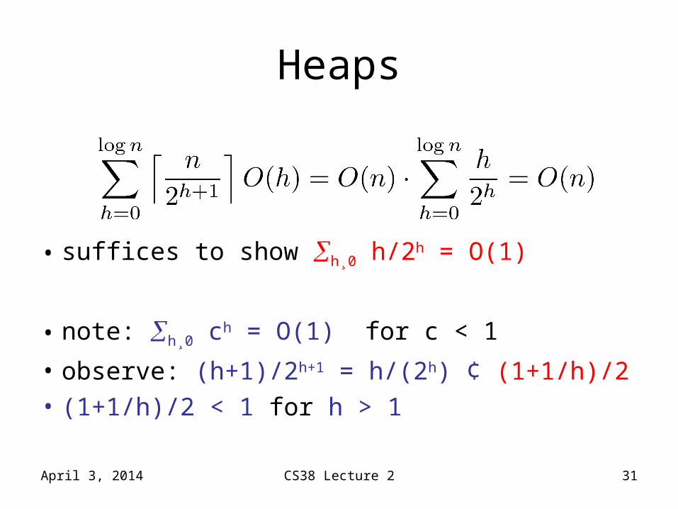
• suffices to show h¸0 h/2h = O(1)
• note: h¸0 ch = O(1) for c < 1
• observe: (h+1)/2h+1 = h/(2h) ¢ (1+1/h)/2
• (1+1/h)/2 < 1 for h > 1April 3, 2014 CS38 Lecture 2 31
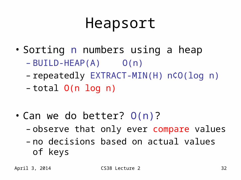
Heapsort
• Sorting n numbers using a heap– BUILD-HEAP(A) O(n)– repeatedly EXTRACT-MIN(H) n
¢O(log n)– total O(n log n)
• Can we do better? O(n)?– observe that only ever compare values – no decisions based on actual values of keys
April 3, 2014 CS38 Lecture 2 32
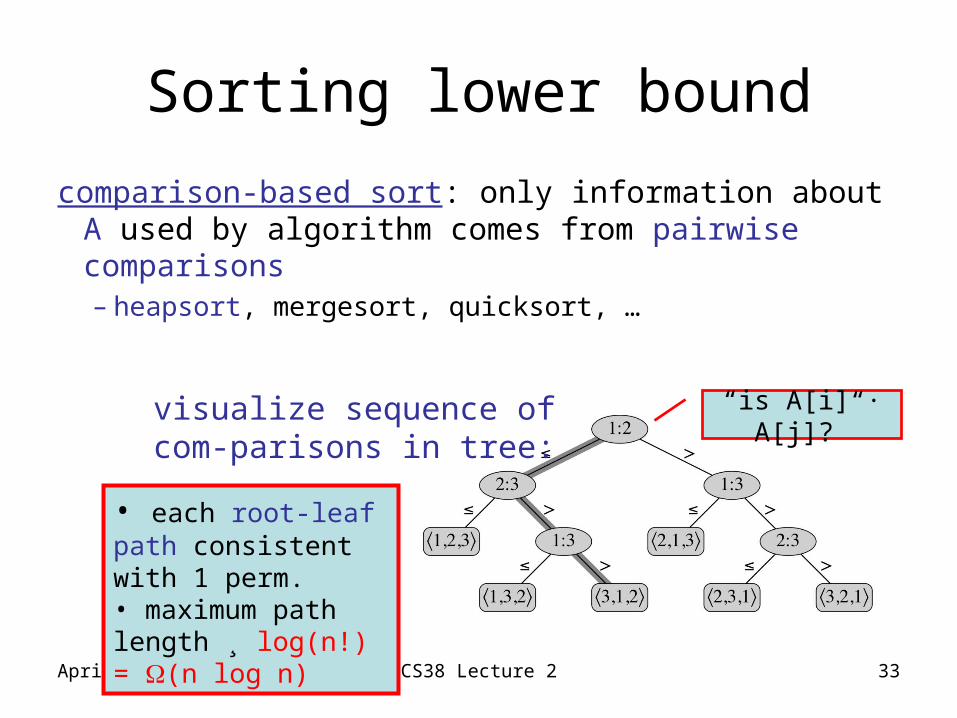
Sorting lower bound
comparison-based sort: only information about A used by algorithm comes from pairwise comparisons– heapsort, mergesort, quicksort, …
April 3, 2014 CS38 Lecture 2 33
visualize sequence of com-parisons in tree:
“is A[i] · A[j]?”
• each root-leaf path consistent with 1 perm.• maximum path length ¸ log(n!) = (n log n)

Greedy
Algorithms
April 3, 2014 CS38 Lecture 2 34
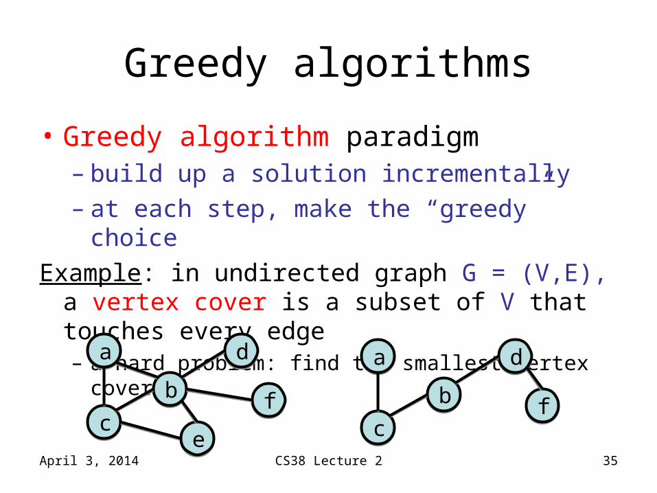
Greedy algorithms
• Greedy algorithm paradigm– build up a solution incrementally– at each step, make the “greedy” choice
Example: in undirected graph G = (V,E), a vertex cover is a subset of V that touches every edge– a hard problem: find the smallest vertex cover
April 3, 2014 CS38 Lecture 2 35
aa
bb
cc
dd
ff
ee
aa
bb
cc
dd
ff
Dijkstra’s algorithm
• given– directed graph G = (V,E) with non-negative
edge weights– starting vertex s 2 V
• find shortest paths from s to all nodes v– note: unweighted case solved by BFS
April 3, 2014 CS38 Lecture 2 36
Dijkstra’s algorithm
• shortest paths exhibit “optimal substructure” property– optimal solution contains within it optimal
solutions to subproblems– a shortest path from x to y via z contains a shortest
path from x to z• shortest paths from s form a tree rooted at s
• Main idea:– maintain set S µ V with correct distances– add nbr u with smallest “distance estimate”
April 3, 2014 CS38 Lecture 2 37
![Algorithms Lecture 1: Recursion [Fa’14] - Jeff Ericksonjeffe.cs.illinois.edu/teaching/algorithms/notes/01-recursion.pdf · Algorithms Lecture 1: Recursion [Fa’14] ... for example](https://img.pdfslide.net/doc/110x75/5ab2eee87f8b9aea528dc5e4/algorithms-lecture-1-recursion-fa14-jeff-lecture-1-recursion-fa14.jpg)