Embed Size (px)
Citation preview
CS38Introduction to Algorithms
Lecture 18
May 29, 2014
May 29, 2014 1CS38 Lecture 18
May 29, 2014 CS38 Lecture 18 2
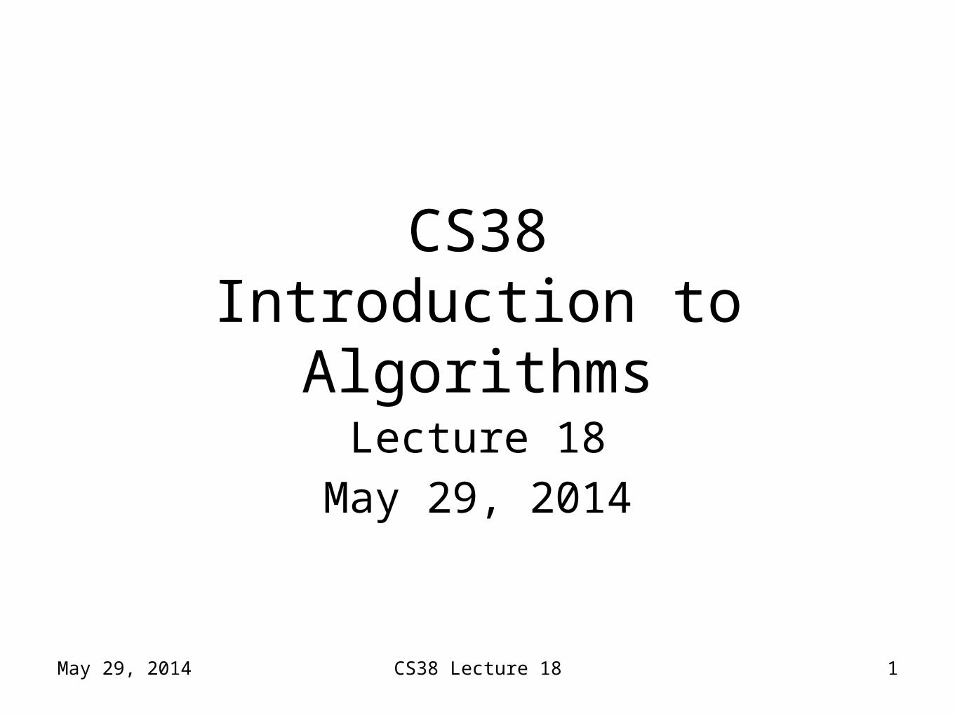
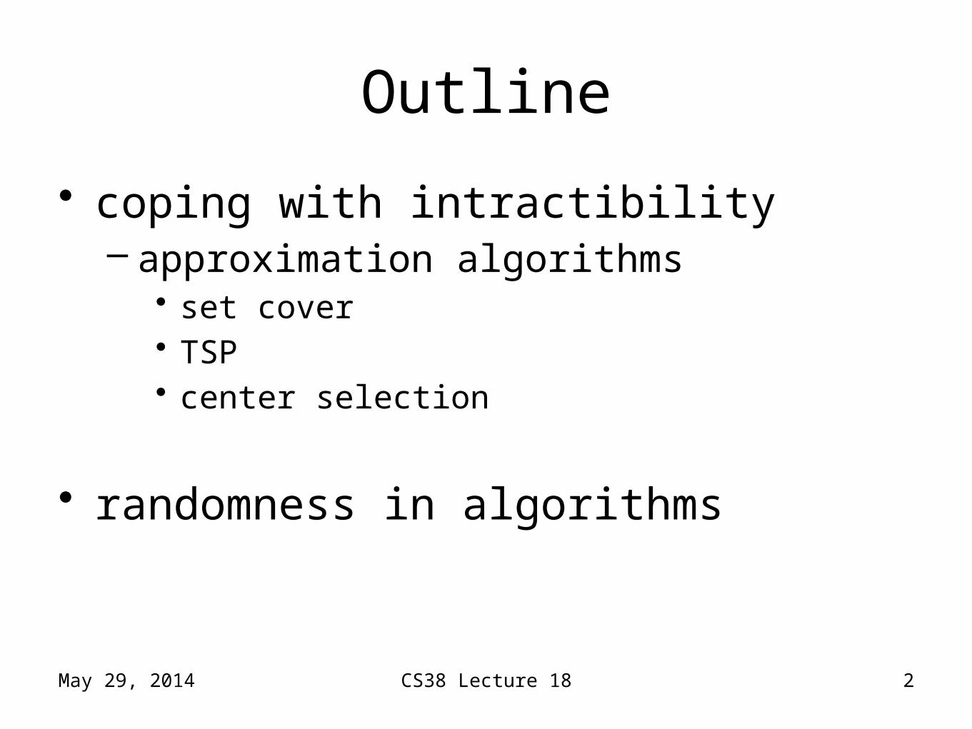
Outline
• coping with intractibility– approximation algorithms
• set cover• TSP• center selection
• randomness in algorithms
May 29, 2014 3
Optimization Problems
• many hard problems (especially NP-hard) are optimization problems– e.g. find shortest TSP tour– e.g. find smallest vertex cover – e.g. find largest clique
– may be minimization or maximization problem– “OPT” = value of optimal solution
CS38 Lecture 18
May 29, 2014 4
Approximation Algorithms
• often happy with approximately optimal solution– warning: lots of heuristics– we want approximation algorithm with
guaranteed approximation ratio of r– meaning: on every input x, output is
guaranteed to have value
at most r*opt for minimization
at least opt/r for maximization
CS38 Lecture 18
Set Cover
• Given subsets S1, S2, …, Sn of a universe U of size m, and an integer k– is there a cover J of size k– “cover”: [j 2J Sj = U
Theorem: set-cover is NP-complete– in NP (why?)– reduce from vertex cover (how?)
May 29, 2014 CS38 Lecture 18 5

Set cover
• Greedy approximation algorithm:– at each step, pick set covering largest number
of remaining uncovered items
Theorem: greedy set cover algorithm achieves an approximation ratio of (ln m + 1)
May 29, 2014 CS38 Lecture 18 6
Set cover
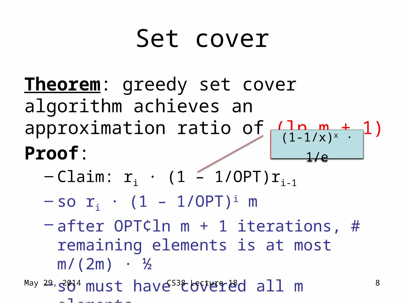
Theorem: greedy set cover algorithm achieves an approximation ratio of (ln m + 1)
Proof:– let ri be # of items remaining after iteration i
– r0 = |U| = m
– Claim: ri · (1 – 1/OPT)ri-1
• proof: OPT sets cover all remaining items so some set covers at least 1/OPT fraction
May 29, 2014 CS38 Lecture 18 7
Set cover
Theorem: greedy set cover algorithm achieves an approximation ratio of (ln m + 1)
Proof:– Claim: ri · (1 – 1/OPT)ri-1
– so ri · (1 – 1/OPT)i m
– after OPT¢ln m + 1 iterations, # remaining elements is at most m/(2m) · ½
– so must have covered all m elements.
May 29, 2014 CS38 Lecture 18 8
(1-1/x)x · 1/e
Travelling Salesperson Problem
• given a complete graph and edge weights satisfying the triangle inequality
wa,b + wb,c ¸ wa,c for all vertices a,b,c
– find a shortest tour that visits every vertex
Theorem: TSP with triangle inequality is NP-complete
– in NP (why?)– reduce from Hamilton cycle (how?)
May 29, 2014 CS38 Lecture 18 9
TSP approximation algorithm
• two key observations:– tour that visits vertices more than once can be
short-circuited without increasing cost, by triangle inequality• short-circuit = skip already-visited vertices
– (multi-)graph with all even degrees has Eulerian tour: a tour that uses all edges• proof?
May 29, 2014 CS38 Lecture 18 10
TSP approximation algorithm
• First approximation algorithm:– find a Minimum Spanning Tree T– double all the edges– output an Euler tour (with short-circuiting)
Theorem: this approximation algorithm achieves approximation ratio 2
May 29, 2014 CS38 Lecture 18 11
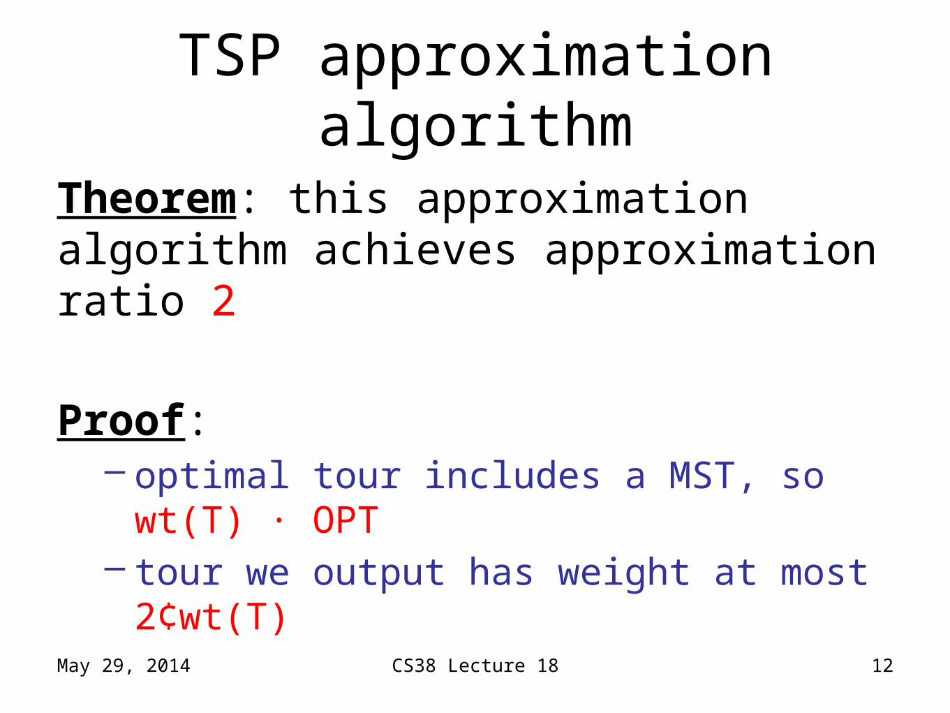
TSP approximation algorithm
Theorem: this approximation algorithm achieves approximation ratio 2
Proof: – optimal tour includes a MST, so wt(T) · OPT– tour we output has weight at most 2¢wt(T)
May 29, 2014 CS38 Lecture 18 12
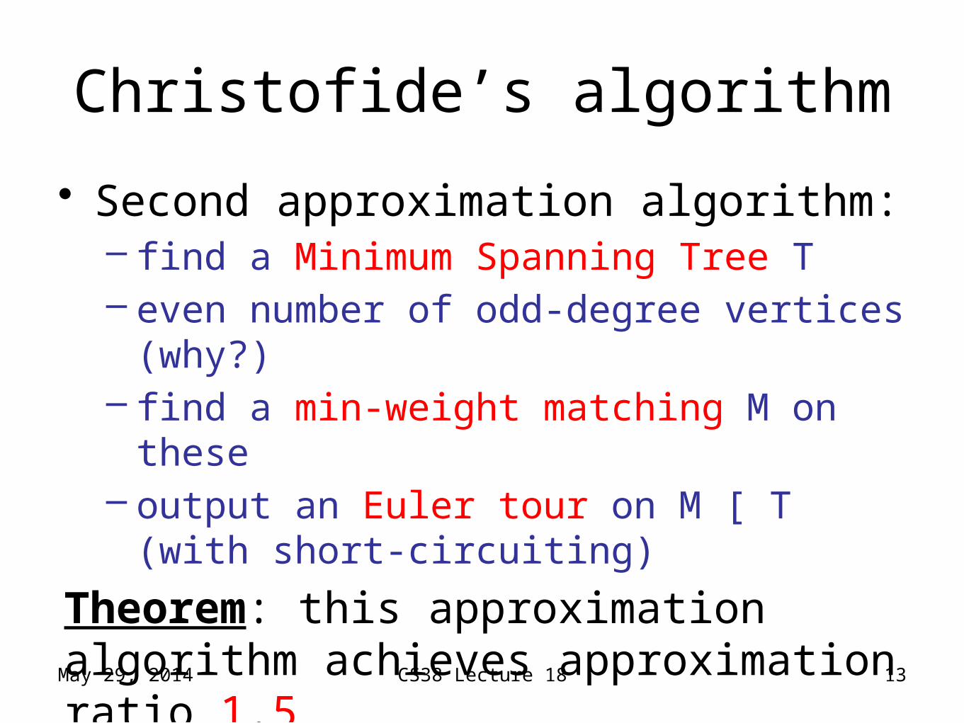
Christofide’s algorithm
• Second approximation algorithm:– find a Minimum Spanning Tree T– even number of odd-degree vertices (why?)– find a min-weight matching M on these– output an Euler tour on M [ T (with short-
circuiting)
Theorem: this approximation algorithm achieves approximation ratio 1.5
May 29, 2014 CS38 Lecture 18 13
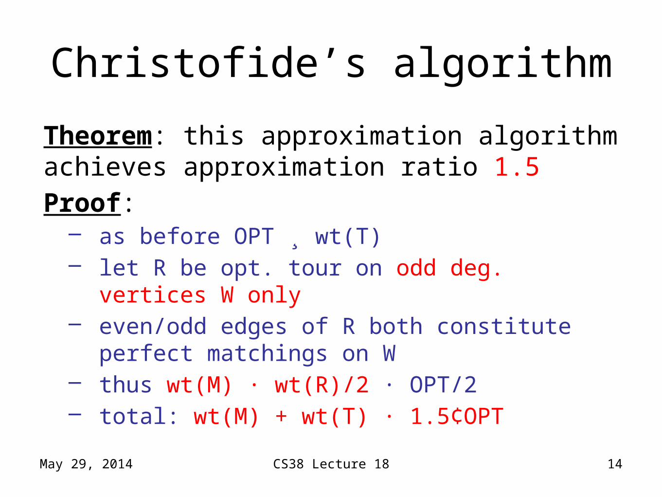
Christofide’s algorithm
Theorem: this approximation algorithm achieves approximation ratio 1.5
Proof:– as before OPT ¸ wt(T)– let R be opt. tour on odd deg. vertices W only – even/odd edges of R both constitute perfect
matchings on W– thus wt(M) · wt(R)/2 · OPT/2 – total: wt(M) + wt(T) · 1.5¢OPT
May 29, 2014 CS38 Lecture 18 14
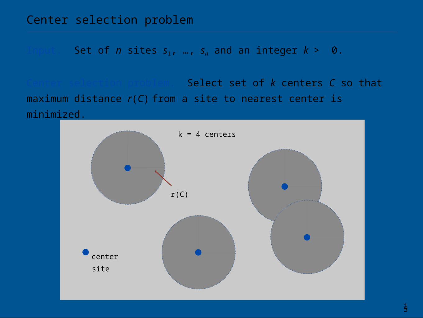
Input. Set of n sites s1, …, sn and an integer k > 0.
Center selection problem. Select set of k centers C so that maximum
distance r(C) from a site to nearest center is minimized.
15
r(C)
Center selection problem
k = 4 centers
center
site
16
Center selection problem
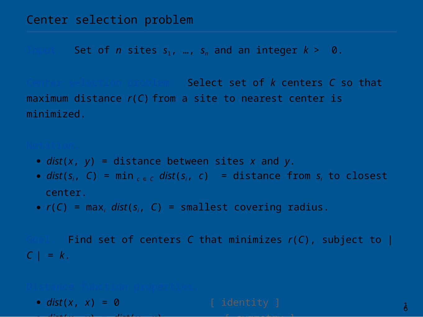
Input. Set of n sites s1, …, sn and an integer k > 0.
Center selection problem. Select set of k centers C so that maximum
distance r(C) from a site to nearest center is minimized.
Notation.
・dist(x, y) = distance between sites x and y.
・dist(si, C) = min c ∈ C dist(si, c) = distance from si to closest center.
・r(C) = maxi dist(si, C) = smallest covering radius.
Goal. Find set of centers C that minimizes r(C), subject to | C | = k.
Distance function properties.
・dist(x, x) = 0 [ identity ]
・dist(x, y) = dist(y, x) [ symmetry ]
・dist(x, y) ≤ dist(x, z) + dist(z, y) [ triangle inequality ]
17
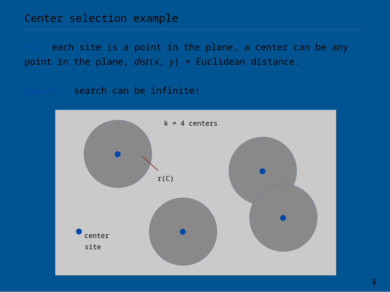
Center selection example
Ex: each site is a point in the plane, a center can be any point in the
plane, dist(x, y) = Euclidean distance.
Remark: search can be infinite!
center
r(C)
site
k = 4 centers
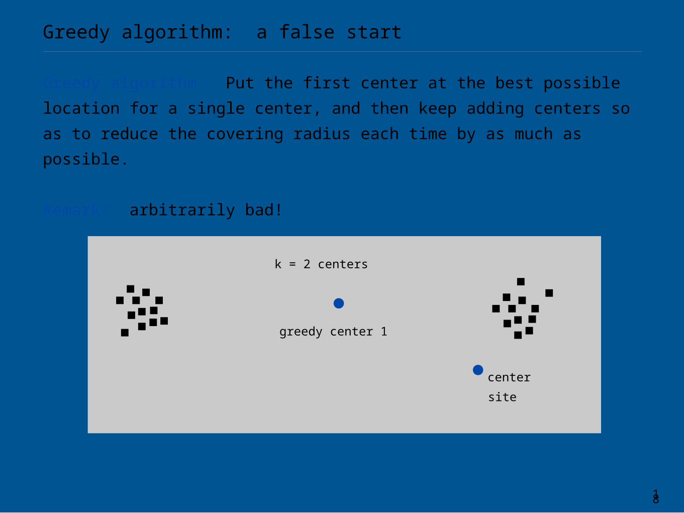
Greedy algorithm. Put the first center at the best possible location for a
single center, and then keep adding centers so as to reduce the covering
radius each time by as much as possible.
Remark: arbitrarily bad!
18
Greedy algorithm: a false start
greedy center 1
center
site
k = 2 centers
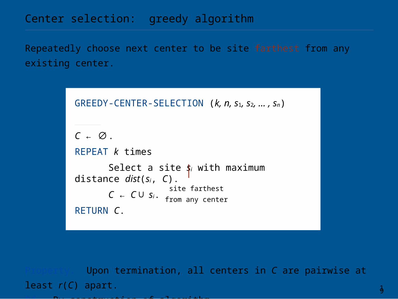
Repeatedly choose next center to be site farthest from any existing
center.
Property. Upon termination, all centers in C are pairwise at least r(C)
apart.
Pf. By construction of algorithm.
GREEDY-CENTER-SELECTION (k, n, s1, s2, … , sn) ________________________________________________________________________________________________________________________________________________________________________________________________________________________________________________________________________________________________________________________________________________________________________________________________________________________________________________________________________________________________________________________________________________________________________________________________________________________________________________________________________________________________________________________________________________________________________________________________________________________________________________________________________________________________________________________________________________________________________________________________________________________________________________________________________________________________________________________________________________________________________
C ← .∅
REPEAT k times
Select a site si with maximum distance dist(si, C).
C ← C ∪ si.
RETURN C.________________________________________________________________________________________________________________________________________________________________________________________________________________________________________________________________________________________________________________________________________________________________________________________________________________________________________________________________________________________________________________________________________________________________________________________________________________________________________________________________________________________________________________________________________________________________________________________________________________________________________________________________________________________________________________________________________________________________________________________________________________________________________________________________________________________________________________________________________________________________________
19
Center selection: greedy algorithm
site farthest
from any center
20
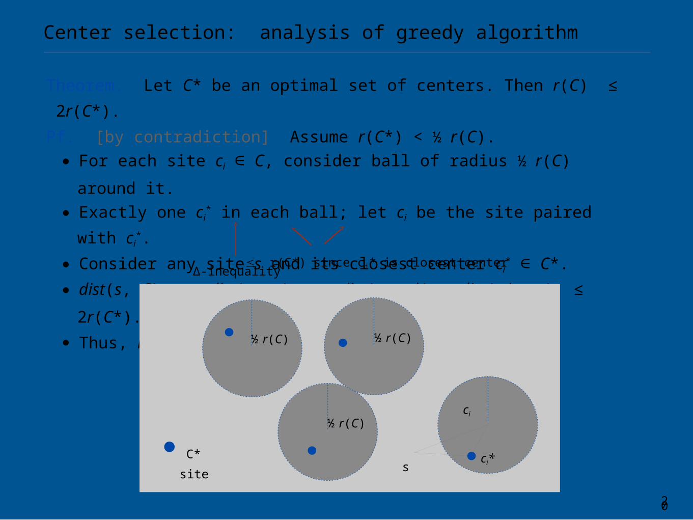
Center selection: analysis of greedy algorithm
Theorem. Let C* be an optimal set of centers. Then r(C) ≤ 2r(C*).
Pf. [by contradiction] Assume r(C*) < ½ r(C).
・For each site ci ∈ C, consider ball of radius ½ r(C) around it.
・Exactly one ci* in each ball; let ci be the site paired with ci
*.
・Consider any site s and its closest center ci* ∈ C*.
・dist(s, C) ≤ dist(s, ci) ≤ dist(s, ci*) + dist(ci*, ci) ≤ 2r(C*).
・Thus, r(C) ≤ 2r(C*). ▪
½ r(C)
ci
ci*s
≤ r(C*) since ci* is closest center
½ r(C)
½ r(C)
Δ-inequality
C*
site
21
Center selection
Lemma. Let C* be an optimal set of centers. Then r(C) ≤ 2r (C*).
Theorem. Greedy algorithm is a 2-approximation for center selection
problem.
Remark. Greedy algorithm always places centers at sites, but is still
within a factor of 2 of best solution that is allowed to place centers
anywhere.
Question. Is there hope of a 3/2-approximation? 4/3?
e.g., points in the plane
Randomness
in algorithms
May 29, 2014 CS38 Lecture 18 22

23
Randomization
Algorithmic design patterns.
・Greedy.
・Divide-and-conquer.
・Dynamic programming.
・Network flow.
・Randomization.
Randomization. Allow fair coin flip in unit time.
Why randomize? Can lead to simplest, fastest, or only known algorithm
for a particular problem.
Ex. Symmetry breaking protocols, graph algorithms, quicksort, hashing,
load balancing, Monte Carlo integration, cryptography.
in practice, access to a pseudo-random number generator

Contention
resolution
May 29, 2014 CS38 Lecture 18 24

25
Contention resolution in a distributed system
Contention resolution. Given n processes P1, …, Pn, each competing for
access to a shared database. If two or more processes access the
database simultaneously, all processes are locked out. Devise protocol to
ensure all processes get through on a regular basis.
Restriction. Processes can't communicate.
Challenge. Need symmetry-breaking paradigm.
P1
P2
Pn
.
.
.
26
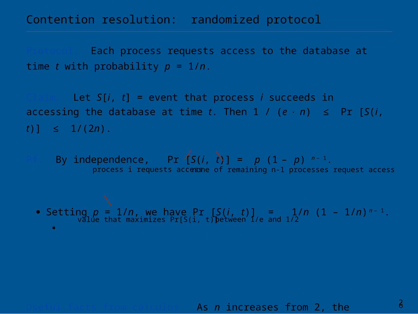
Contention resolution: randomized protocol
Protocol. Each process requests access to the database at time t with
probability p = 1/n.
Claim. Let S[i, t] = event that process i succeeds in accessing the
database at time t. Then 1 / (e ⋅ n) ≤ Pr [S(i, t)] ≤ 1/(2n).
Pf. By independence, Pr [S(i, t)] = p (1 – p) n – 1.
・Setting p = 1/n, we have Pr [S(i, t)] = 1/n (1 – 1/n) n – 1. ▪
Useful facts from calculus. As n increases from 2, the function:
・(1 – 1/n) n -1 converges monotonically from 1/4 up to 1 / e.
・(1 – 1/n) n – 1 converges monotonically from 1/2 down to 1 / e.
process i requests access none of remaining n-1 processes request access
value that maximizes Pr[S(i, t)] between 1/e and 1/2
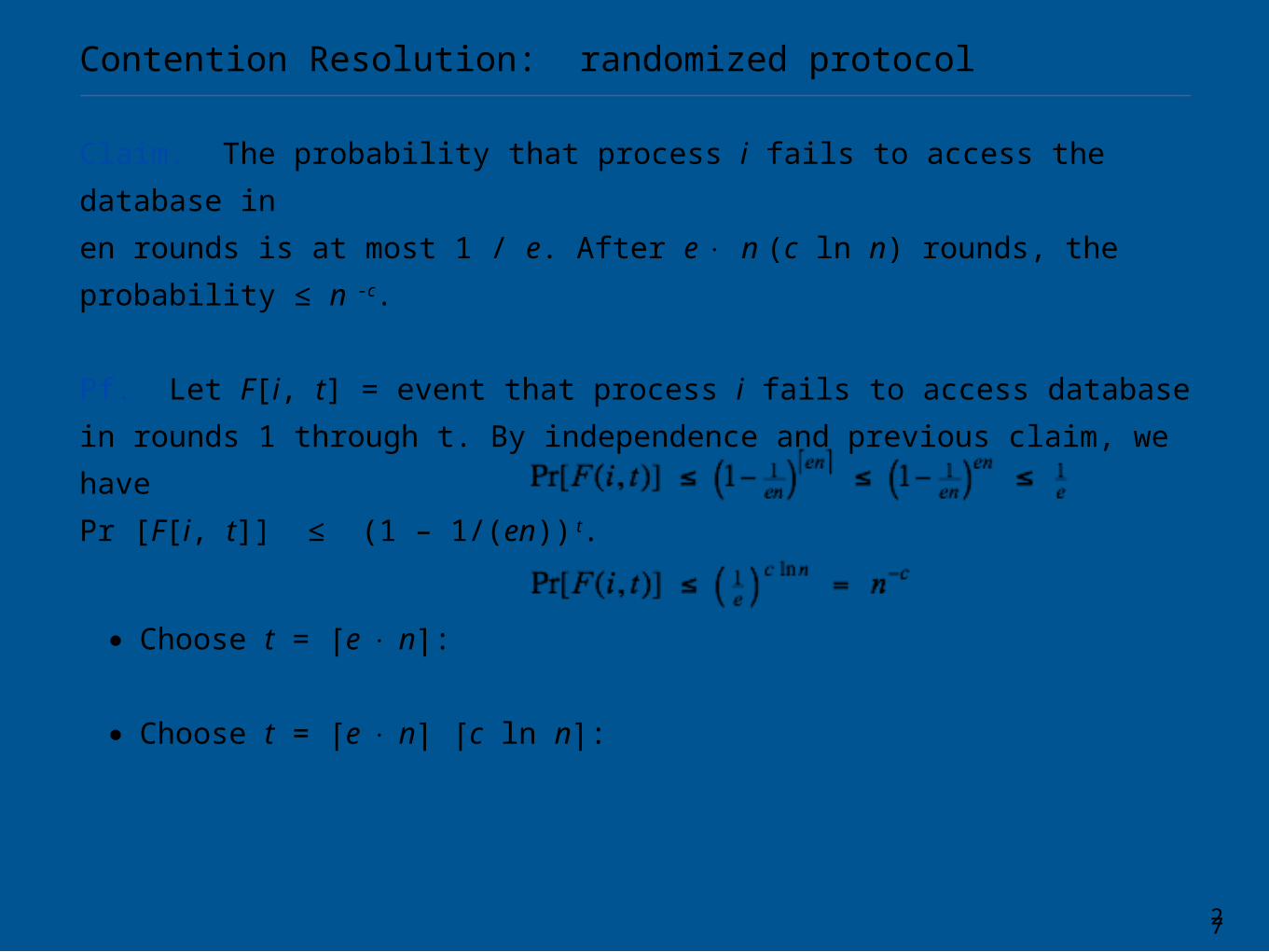
Claim. The probability that process i fails to access the database in
en rounds is at most 1 / e. After e ⋅ n (c ln n) rounds, the probability ≤ n -c.
Pf. Let F[i, t] = event that process i fails to access database in rounds 1
through t. By independence and previous claim, we have
Pr [F[i, t]] ≤ (1 – 1/(en)) t.
・Choose t = ⎡e ⋅ n⎤:
・Choose t = ⎡e ⋅ n⎤ ⎡c ln n⎤:
27
Contention Resolution: randomized protocol

28
Contention Resolution: randomized protocol
Claim. The probability that all processes succeed within 2e ⋅ n ln n rounds
is ≥ 1 – 1 / n.
Pf. Let F[t] = event that at least one of the n processes fails to access
database in any of the rounds 1 through t.
・Choosing t = 2 ⎡en⎤ ⎡c ln n⎤ yields Pr[F[t]] ≤ n · n-2 = 1 / n. ▪
Union bound. Given events E1, …, En,
union bound previous slide

Global
min cut
May 29, 2014 CS38 Lecture 18 29
30
Global minimum cut
Global min cut. Given a connected, undirected graph G = (V, E),
find a cut (A, B) of minimum cardinality.
Applications. Partitioning items in a database, identify clusters of related
documents, network reliability, network design, circuit design, TSP
solvers.
Network flow solution.
・Replace every edge (u, v) with two antiparallel edges (u, v) and (v, u).
・Pick some vertex s and compute min s- v cut separating s from each
other vertex v ∈ V.
False intuition. Global min-cut is harder than min s-t cut.
31
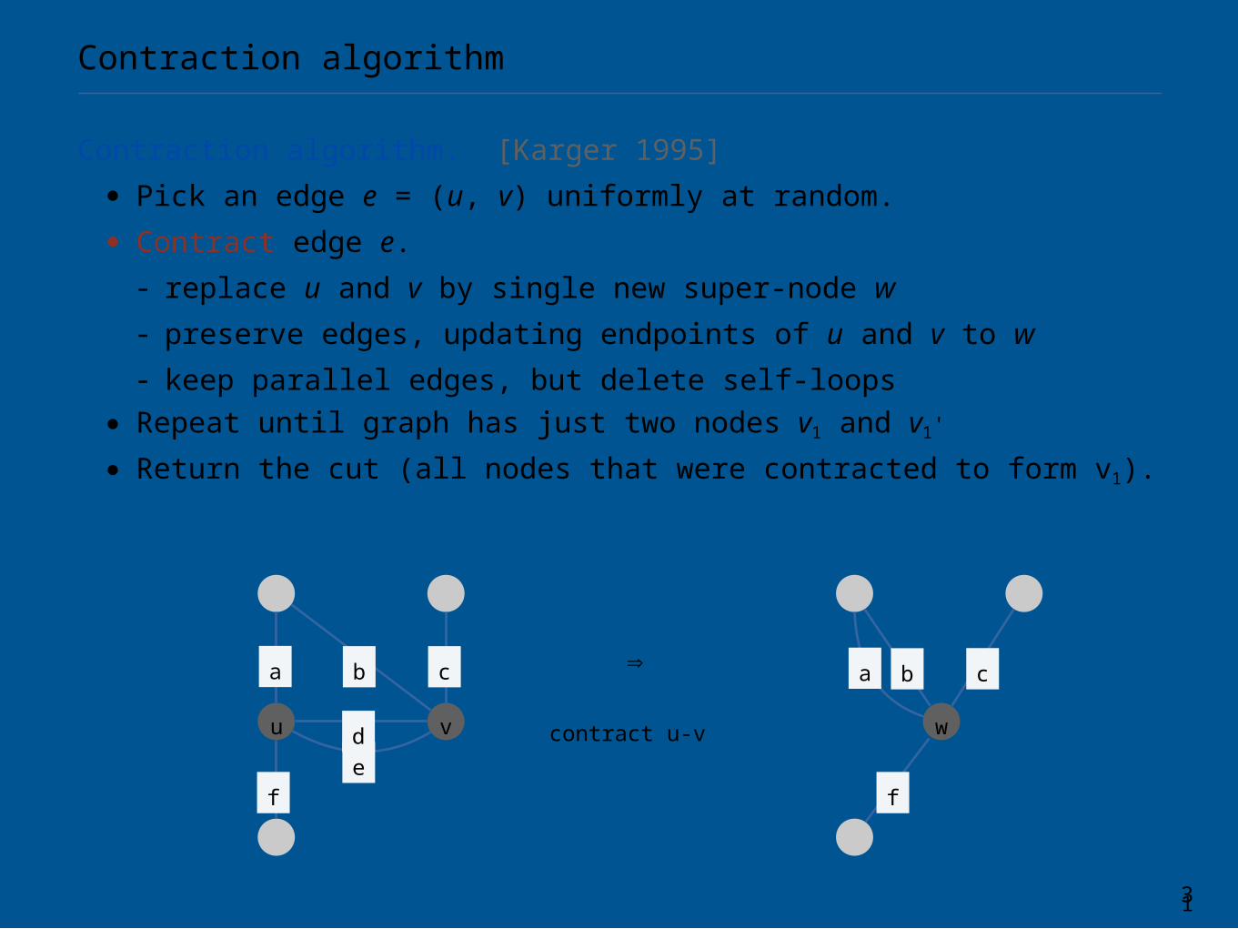
Contraction algorithm
Contraction algorithm. [Karger 1995]
・Pick an edge e = (u, v) uniformly at random.
・Contract edge e.
- replace u and v by single new super-node w
- preserve edges, updating endpoints of u and v to w
- keep parallel edges, but delete self-loops
・Repeat until graph has just two nodes v1 and v1'
・Return the cut (all nodes that were contracted to form v1).
u v w
⇒
contract u-v
a b c
ef
ca b
f
d
32
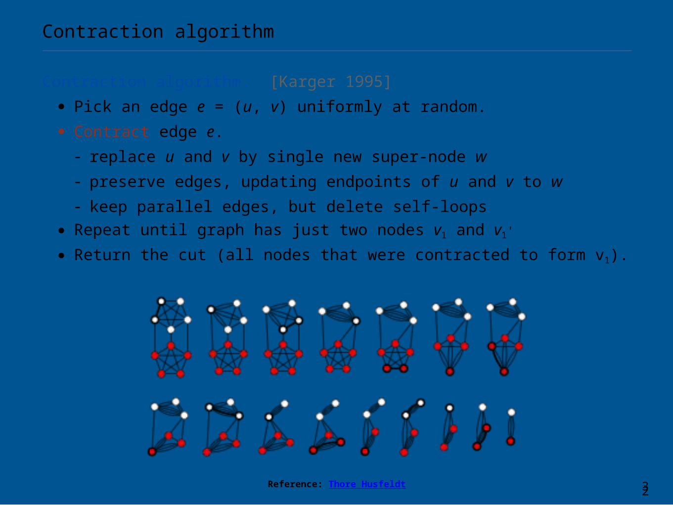
Contraction algorithm
Contraction algorithm. [Karger 1995]
・Pick an edge e = (u, v) uniformly at random.
・Contract edge e.
- replace u and v by single new super-node w
- preserve edges, updating endpoints of u and v to w
- keep parallel edges, but delete self-loops
・Repeat until graph has just two nodes v1 and v1'
・Return the cut (all nodes that were contracted to form v1).
Reference: Thore Husfeldt
33
Contraction algorithm
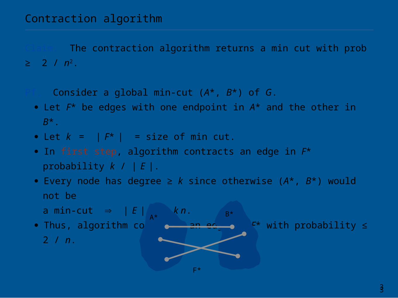
Claim. The contraction algorithm returns a min cut with prob ≥ 2 / n2.
Pf. Consider a global min-cut (A*, B*) of G.
・Let F* be edges with one endpoint in A* and the other in B*.
・Let k = | F* | = size of min cut.
・In first step, algorithm contracts an edge in F* probability k / | E |.
・Every node has degree ≥ k since otherwise (A*, B*) would not be
a min-cut ⇒ | E | ≥ ½ k n.
・Thus, algorithm contracts an edge in F* with probability ≤ 2 / n.
A* B*
F*
34
Contraction algorithm
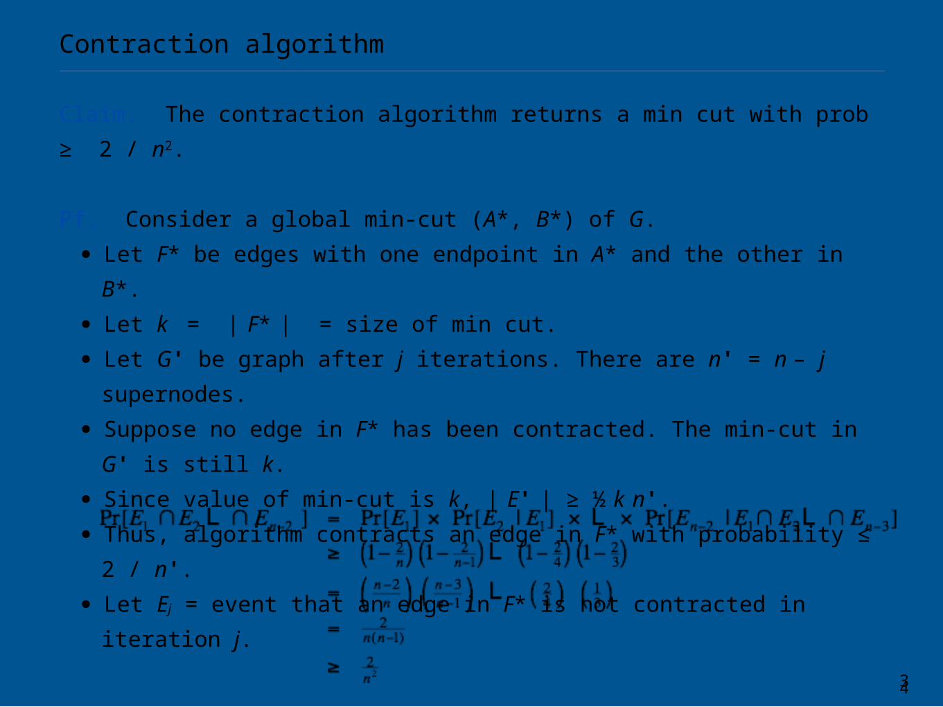
Claim. The contraction algorithm returns a min cut with prob ≥ 2 / n2.
Pf. Consider a global min-cut (A*, B*) of G.
・Let F* be edges with one endpoint in A* and the other in B*.
・Let k = | F* | = size of min cut.
・Let G' be graph after j iterations. There are n' = n – j supernodes.
・Suppose no edge in F* has been contracted. The min-cut in G' is still
k.
・Since value of min-cut is k, | E' | ≥ ½ k n'.
・Thus, algorithm contracts an edge in F* with probability ≤ 2 / n'.
・Let Ej = event that an edge in F* is not contracted in iteration j.
35
Contraction algorithm
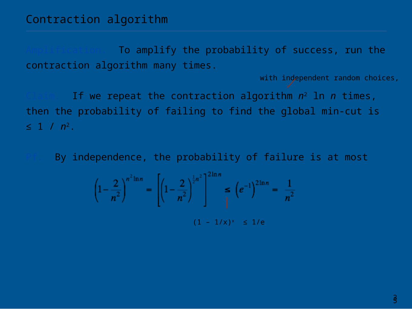
Amplification. To amplify the probability of success, run the contraction
algorithm many times.
Claim. If we repeat the contraction algorithm n2 ln n times,
then the probability of failing to find the global min-cut is ≤ 1 / n2.
Pf. By independence, the probability of failure is at most
(1 – 1/x)x ≤ 1/e
with independent random choices,

36
Contraction algorithm: example execution
trial 1
trial 2
trial 3
trial 4
trial 5
(finds min cut)
trial 6
...Reference: Thore Husfeldt
37
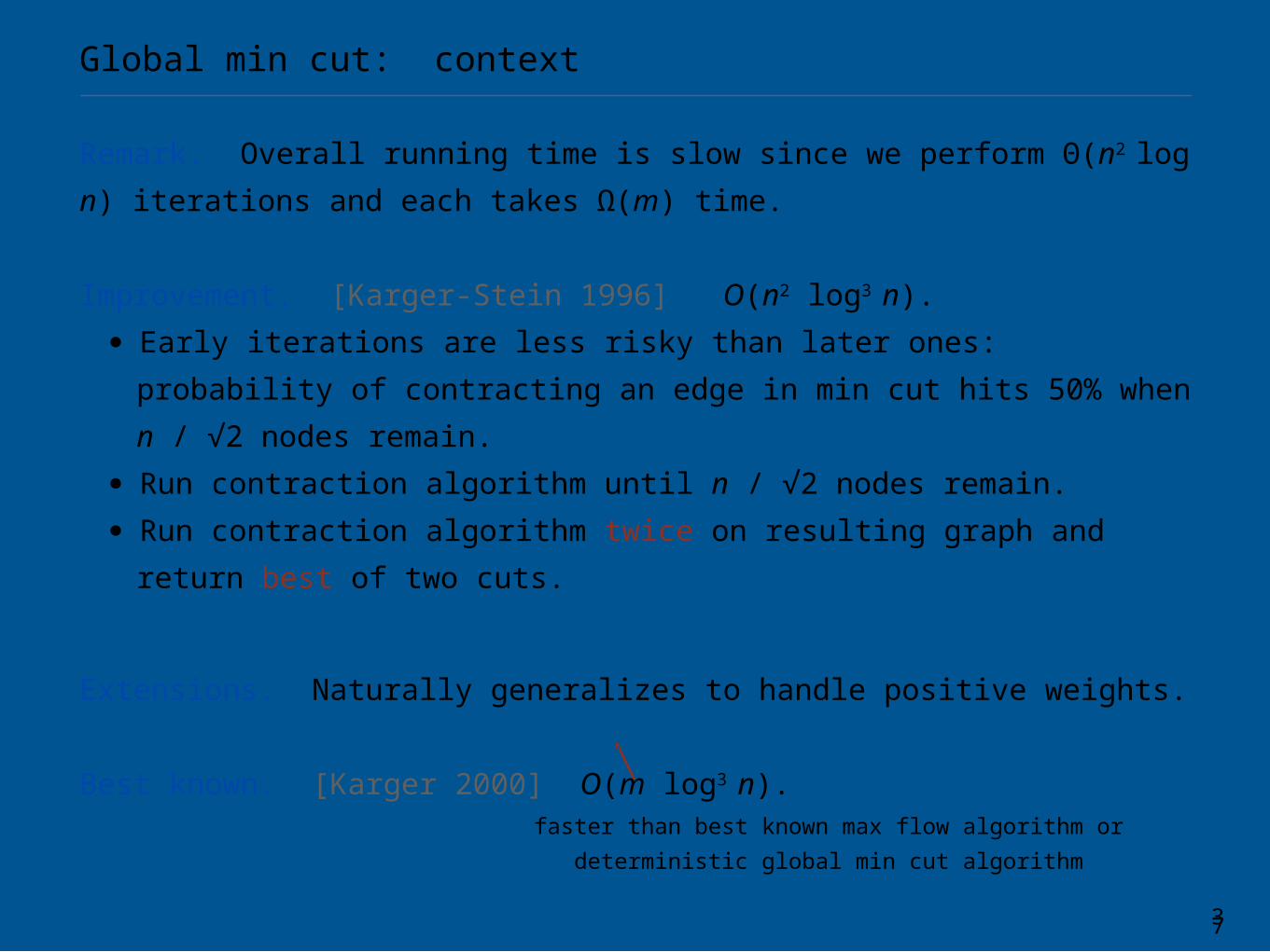
Global min cut: context
Remark. Overall running time is slow since we perform Θ(n2 log n)
iterations and each takes Ω(m) time.
Improvement. [Karger-Stein 1996] O(n2 log3 n).
・Early iterations are less risky than later ones: probability of
contracting an edge in min cut hits 50% when n / √2 nodes remain.
・Run contraction algorithm until n / √2 nodes remain.
・Run contraction algorithm twice on resulting graph and
return best of two cuts.
Extensions. Naturally generalizes to handle positive weights.
Best known. [Karger 2000] O(m log3 n).
faster than best known max flow algorithm or
deterministic global min cut algorithm