Embed Size (px)
Citation preview
Consortium for Advanced Simulation of LWRs
CASL-U-2015-0320-002
CTF Void Drift Validation Study
Robert Salko, Oak Ridge National Laboratory Marcus Gergar, The Pennsylvania State University Chris Gosdin, The Pennsylvania State University Maria Avramova, North Carolina State University 10/26/2015
ORNL/SR-2015/641
Approved for public release.Distribution is unlimited.

CASL-U-2015-0320-002 Page ii
REVISION LOG Revision Date Affected Pages Revision Description
0 9/30/15 All Initial Release
1 10/05/15 All Adding mixing validation and more GE 3×3 tests
2 10/26/15 All Addressing reviewer comments
Document pages that are:
Export Controlled __________________________________________________ IP/Proprietary/NDA Controlled__ ____________________________________
Sensitive Controlled________________________________________________
Requested Distribution: To: Richard Lahey, Kevin Clarno, Scott Palmtag
Copy: Jeff Banta
CTF Void Fraction Validation
EXECUTIVE SUMMARY
This milestone report is a summary of work performed in support of expansion of the validation andverification (V&V) matrix for the thermal-hydraulic subchannel code, CTF. The focus of this studyis on validating the void drift modeling capabilities of CTF and verifying the supporting modelsthat impact the void drift phenomenon. CTF uses a simple turbulent-diffusion approximation tomodel lateral cross-flow due to turbulent mixing and void drift. The void drift component of themodel is based on the Lahey and Moody model. The models are a function of two-phase mass,momentum, and energy distribution in the system; therefore, it is necessary to correctly model theflow distribution in rod bundle geometry as a first step to correctly calculating the void distributiondue to void drift. Considering this, a stepwise approach is taken to validate the void drift model inCTF by ensuring
1. the single-phase flow distribution is correctly predicted compared with an analytical solution,
2. the single-phase mixing is correctly predicted compared with an analytical solution,
3. the calculated flow distribution compares well with experimental single-phase data, and
4. the calculated void distribution compares favorably with experimental data.
The existing CTF Validation Manual already contains void-drift validation data using the Gen-eral Electric (GE) 3×3 facility to address Item 4 in the above list. This study addresses Items 1–3and expands on Item 4 using new data. The first attempt at this expansion involved modeling the2×2 air/water facility operated at Rensselaer Polytechnic Institute (RPI). However, it is discoveredthat CTF has a great deal of difficulty in converging this case likely due to the large geometry, lowpressure, and two-phase injection. To better address Item 4, the Boiling Water Reactor Full-SizeFine-Mesh Bundle Test (BFBT) void distribution cases are run with CTF, which are steam/watertwo-phase tests run at prototypical BWR operating conditions in an 8×8 rod-bundle facility. Addi-tionally, the GE 3×3 validation study is expanded with new test cases as well as additional analysis.
CASL-U-2015-0320-002 iii Consortium for Advanced Simulation of LWRs

This page intentionally left blank
CTF Void Fraction Validation
CONTENTS
EXECUTIVE SUMMARY iii
CONTENTS v
FIGURES vi
TABLES ix
ACRONYMS x
1 INTRODUCTION 1
2 SINGLE-PHASE FLOW DISTRIBUTION TESTING 22.1 Two-Channel Friction Model Verification . . . . . . . . . . . . . . . . . . . . . . . . 32.2 Turbulent Mixing Verification . . . . . . . . . . . . . . . . . . . . . . . . . . . . . . . 62.3 2×3 Validation . . . . . . . . . . . . . . . . . . . . . . . . . . . . . . . . . . . . . . . 112.4 RPI 2×2 Validation . . . . . . . . . . . . . . . . . . . . . . . . . . . . . . . . . . . . 152.5 GE 3×3 Validation . . . . . . . . . . . . . . . . . . . . . . . . . . . . . . . . . . . . . 24
3 VOID DRIFT VALIDATION 313.1 RPI 2×2 Validation . . . . . . . . . . . . . . . . . . . . . . . . . . . . . . . . . . . . 313.2 GE 3×3 Validation . . . . . . . . . . . . . . . . . . . . . . . . . . . . . . . . . . . . . 383.3 BWR Full-Size Fine-Mesh Bundle Test (BFBT) 8×8 Validation . . . . . . . . . . . . 46
4 CONCLUSION 80
CASL-U-2015-0320-002 v Consortium for Advanced Simulation of LWRs

CTF Void Fraction Validation
FIGURES
1 Diagram of the two-channel flow split problem. . . . . . . . . . . . . . . . . . . . . . 52 Two-channel flow-split results . . . . . . . . . . . . . . . . . . . . . . . . . . . . . . . 63 Model of problem for testing single-phase turbulent mixing of enthalpy. . . . . . . . 74 Turbulent-mixing problem results . . . . . . . . . . . . . . . . . . . . . . . . . . . . . 105 Mixing problem mass flow rates . . . . . . . . . . . . . . . . . . . . . . . . . . . . . . 106 Mixing problem mass flow rates with no mixing . . . . . . . . . . . . . . . . . . . . . 117 2×3 facility cross section . . . . . . . . . . . . . . . . . . . . . . . . . . . . . . . . . . 128 2×3 facility side view . . . . . . . . . . . . . . . . . . . . . . . . . . . . . . . . . . . . 129 2×3 opearting conditions . . . . . . . . . . . . . . . . . . . . . . . . . . . . . . . . . 1410 2×3 results using Rogers and Rosehart . . . . . . . . . . . . . . . . . . . . . . . . . . 1411 2×3 results using β=0.004 . . . . . . . . . . . . . . . . . . . . . . . . . . . . . . . . . 1612 2×3 results using β=0.007 . . . . . . . . . . . . . . . . . . . . . . . . . . . . . . . . . 1613 2×3 results using CTF friction model . . . . . . . . . . . . . . . . . . . . . . . . . . 1714 Watts Bar simulation sensitivity to β . . . . . . . . . . . . . . . . . . . . . . . . . . . 1715 2×2 Case 1 results with no mixing . . . . . . . . . . . . . . . . . . . . . . . . . . . . 2016 2×2 Case 2 results with no mixing . . . . . . . . . . . . . . . . . . . . . . . . . . . . 2017 2×2 Case 1 results with mixing . . . . . . . . . . . . . . . . . . . . . . . . . . . . . . 2118 2×2 Case 2 results with mixing . . . . . . . . . . . . . . . . . . . . . . . . . . . . . . 2119 2×2 Case 1 results with β perturbation . . . . . . . . . . . . . . . . . . . . . . . . . 2320 2×2 Case 2 results with β perturbation . . . . . . . . . . . . . . . . . . . . . . . . . 2321 GE 3×3 Case 1B results with no mixing . . . . . . . . . . . . . . . . . . . . . . . . . 2522 GE 3×3 Case 1C results with no mixing . . . . . . . . . . . . . . . . . . . . . . . . . 2523 GE 3×3 Case 1D results with no mixing . . . . . . . . . . . . . . . . . . . . . . . . . 2624 GE 3×3 Case 1E results with no mixing . . . . . . . . . . . . . . . . . . . . . . . . . 2625 GE 3×3 Case 1B results with mixing . . . . . . . . . . . . . . . . . . . . . . . . . . . 2726 GE 3×3 Case 1C results with mixing . . . . . . . . . . . . . . . . . . . . . . . . . . . 2727 GE 3×3 Case 1D results with mixing . . . . . . . . . . . . . . . . . . . . . . . . . . . 2828 GE 3×3 Case 1E results with mixing . . . . . . . . . . . . . . . . . . . . . . . . . . . 2829 GE 3×3 single-phase test summary . . . . . . . . . . . . . . . . . . . . . . . . . . . . 3030 GE 3×3 single-phase test summary using Rogers and Rosehart . . . . . . . . . . . . 3031 CTF convergence terms for Test 3 of the 2×2 facility when run at atmospheric pressure. 3232 Exit void in Test 3 of 2×2 facility throughout simulation. . . . . . . . . . . . . . . . 3233 Exit void in Test 3 of 2×2 facility with gaps disabled. . . . . . . . . . . . . . . . . . 3334 2×2 Test 3 50 bar low void . . . . . . . . . . . . . . . . . . . . . . . . . . . . . . . . 3335 2×2 Test 3 50 bar high void . . . . . . . . . . . . . . . . . . . . . . . . . . . . . . . . 3436 2×2 Test 3 100 bar low void . . . . . . . . . . . . . . . . . . . . . . . . . . . . . . . . 3437 2×2 Test 3 100 bar medium void . . . . . . . . . . . . . . . . . . . . . . . . . . . . . 3538 2×2 Test 3 100 bar high void . . . . . . . . . . . . . . . . . . . . . . . . . . . . . . . 3539 2×2 Test 3 100 bar void at 0.4 . . . . . . . . . . . . . . . . . . . . . . . . . . . . . . 3640 2×2 predicted flow split . . . . . . . . . . . . . . . . . . . . . . . . . . . . . . . . . . 3741 2×2 predicted flow split in extended model . . . . . . . . . . . . . . . . . . . . . . . 3742 2×2 Test 3 void for extended facility . . . . . . . . . . . . . . . . . . . . . . . . . . . 3843 GE 3×3 quality summary . . . . . . . . . . . . . . . . . . . . . . . . . . . . . . . . . 4044 GE 3×3 quality summary without void drift . . . . . . . . . . . . . . . . . . . . . . . 4045 GE 3×3 mass flux summary . . . . . . . . . . . . . . . . . . . . . . . . . . . . . . . . 4146 GE 3×3 mass flux summary without void drift . . . . . . . . . . . . . . . . . . . . . 4147 GE 3×3 mass flux summary using Rogers and Rosehart . . . . . . . . . . . . . . . . 4248 GE 3×3 quality summary using Rogers and Rosehart . . . . . . . . . . . . . . . . . . 4249 GE 3×3 Case 2C1 flow split . . . . . . . . . . . . . . . . . . . . . . . . . . . . . . . . 4450 GE 3×3 Case 2C2 flow split . . . . . . . . . . . . . . . . . . . . . . . . . . . . . . . . 4451 GE 3×3 Case 2G1 flow split . . . . . . . . . . . . . . . . . . . . . . . . . . . . . . . . 4552 GE 3×3 Case 2D3 flow split . . . . . . . . . . . . . . . . . . . . . . . . . . . . . . . . 45
Consortium for Advanced Simulation of LWRs vi CASL-U-2015-0320-002

CTF Void Fraction Validation
53 Assembly 0-1, 0-2, and 0-3 description . . . . . . . . . . . . . . . . . . . . . . . . . . 4754 Assembly 0-1, 0-2, and 0-3 description (continued) . . . . . . . . . . . . . . . . . . . 4855 Assembly 1, 2, and 3 description . . . . . . . . . . . . . . . . . . . . . . . . . . . . . 4856 Assembly 1 power . . . . . . . . . . . . . . . . . . . . . . . . . . . . . . . . . . . . . 4957 Assembly 4 power . . . . . . . . . . . . . . . . . . . . . . . . . . . . . . . . . . . . . 5058 Assembly 4 description . . . . . . . . . . . . . . . . . . . . . . . . . . . . . . . . . . . 5059 BFBT void measurements . . . . . . . . . . . . . . . . . . . . . . . . . . . . . . . . . 5160 Assembly 0-1, 0-2, 0-3, and 1 flow areas . . . . . . . . . . . . . . . . . . . . . . . . . 5161 Assembly 4 flow areas . . . . . . . . . . . . . . . . . . . . . . . . . . . . . . . . . . . 5262 C2A ferrule grid geometry . . . . . . . . . . . . . . . . . . . . . . . . . . . . . . . . . 5363 BFBT loss coefficients . . . . . . . . . . . . . . . . . . . . . . . . . . . . . . . . . . . 5464 Comparison of measured and predicted bundle-averaged outlet void. . . . . . . . . . 5565 Comparison of measured and predicted bundle-averaged outlet thermal equilibrium
quality. . . . . . . . . . . . . . . . . . . . . . . . . . . . . . . . . . . . . . . . . . . . 5566 Assembly 0-1 void . . . . . . . . . . . . . . . . . . . . . . . . . . . . . . . . . . . . . 5767 Assembly 0-2 void . . . . . . . . . . . . . . . . . . . . . . . . . . . . . . . . . . . . . 5768 Assembly 0-3 void . . . . . . . . . . . . . . . . . . . . . . . . . . . . . . . . . . . . . 5869 Assembly 1 void . . . . . . . . . . . . . . . . . . . . . . . . . . . . . . . . . . . . . . 5870 Assembly 4 void . . . . . . . . . . . . . . . . . . . . . . . . . . . . . . . . . . . . . . 5971 BFBT void summary . . . . . . . . . . . . . . . . . . . . . . . . . . . . . . . . . . . . 6072 BFBT void summary with droplets . . . . . . . . . . . . . . . . . . . . . . . . . . . . 6073 BFBT corner channel void . . . . . . . . . . . . . . . . . . . . . . . . . . . . . . . . . 6174 BFBT corner channel void with droplets . . . . . . . . . . . . . . . . . . . . . . . . . 6175 BFBT side channel void . . . . . . . . . . . . . . . . . . . . . . . . . . . . . . . . . . 6276 BFBT side channel void with droplets . . . . . . . . . . . . . . . . . . . . . . . . . . 6277 BFBT inner channel void . . . . . . . . . . . . . . . . . . . . . . . . . . . . . . . . . 6378 BFBT inner channel void with droplets . . . . . . . . . . . . . . . . . . . . . . . . . 6379 BFBT unheated channel void . . . . . . . . . . . . . . . . . . . . . . . . . . . . . . . 6480 BFBT unheated channel void with droplets . . . . . . . . . . . . . . . . . . . . . . . 6481 BFBT void with no void drift . . . . . . . . . . . . . . . . . . . . . . . . . . . . . . . 6582 BFBT corner void with no void drift . . . . . . . . . . . . . . . . . . . . . . . . . . . 6583 BFBT side void with no void drift . . . . . . . . . . . . . . . . . . . . . . . . . . . . 6684 BFBT inner void with no void drift . . . . . . . . . . . . . . . . . . . . . . . . . . . . 6685 BFBT unheated void with no void drift . . . . . . . . . . . . . . . . . . . . . . . . . 6786 Example of diagonal lines from where subchannel void data is extracted. . . . . . . . 6987 Measured and predicted void along diagonals of Test 0011-55. . . . . . . . . . . . . . 7088 Measured and predicted void along diagonals of Test 0011-55 with void drift disabled. 7089 Measured and predicted void along diagonals of Test 0011-61. . . . . . . . . . . . . . 7190 Measured and predicted void along diagonals of Test 0011-61 with void drift disabled. 7191 Measured and predicted void along diagonals of Test 0021-16. . . . . . . . . . . . . . 7292 Measured and predicted void along diagonals of Test 0021-16 with void drift disabled. 7293 Measured and predicted void along diagonals of Test 0021-21. . . . . . . . . . . . . . 7394 Measured and predicted void along diagonals of Test 0021-21 with void drift disabled. 7395 Measured and predicted void along diagonals of Test 0031-16. . . . . . . . . . . . . . 7496 Measured and predicted void along diagonals of Test 0031-16 with void drift disabled. 7497 Measured and predicted void along diagonals of Test 0031-21. . . . . . . . . . . . . . 7598 Measured and predicted void along diagonals of Test 0031-21 with void drift disabled. 7599 Measured and predicted void along diagonals of Test 1071-55. . . . . . . . . . . . . . 76100 Measured and predicted void along diagonals of Test 1071-55 with void drift disabled. 76101 Measured and predicted void along diagonals of Test 1071-61. . . . . . . . . . . . . . 77102 Measured and predicted void along diagonals of Test 1071-61 with void drift disabled. 77103 Measured and predicted void along diagonals of Test 4101-53. . . . . . . . . . . . . . 78104 Measured and predicted void along diagonals of Test 4101-53 with void drift disabled. 78105 Measured and predicted void along diagonals of Test 4101-61. . . . . . . . . . . . . . 79
CASL-U-2015-0320-002 vii Consortium for Advanced Simulation of LWRs

CTF Void Fraction Validation
106 Measured and predicted void along diagonals of Test 4101-61 with void drift disabled. 79
Consortium for Advanced Simulation of LWRs viii CASL-U-2015-0320-002

CTF Void Fraction Validation
TABLES
1 NUREG Subchannel Flow Dimensions . . . . . . . . . . . . . . . . . . . . . . . . . . 182 Experimental Operating Conditions . . . . . . . . . . . . . . . . . . . . . . . . . . . 183 BFBT void distribution test conditions . . . . . . . . . . . . . . . . . . . . . . . . . . 474 BFBT Assembly Type 1 axial power distribution. . . . . . . . . . . . . . . . . . . . . 495 Summary of the CTF predictions of BFBT void distribution cases . . . . . . . . . . 67
CASL-U-2015-0320-002 ix Consortium for Advanced Simulation of LWRs
CTF Void Fraction Validation
ACRONYMS
BFBT BWR Full-Size Fine-Mesh Bundle Test
BWR boiling water reactor
GE General Electric
LWR light water reactor
PWR pressurized water reactor
RPI Rensselaer Polytechnic Institute
RMSE root-mean-square of error
rRMSE relative root-mean-square of error
V&V validation and verification
Consortium for Advanced Simulation of LWRs x CASL-U-2015-0320-002

CTF Void Fraction Validation
1 INTRODUCTION
This report documents the annual update to the CTF validation and verification (V&V) test matrix.This update is focused on expanding the testing of the void drift model in CTF as well as thesupporting models that most significantly affect the phenomena. CTF uses a simple diffusion modelbased on mixing-length theory for capturing turbulent mixing and void drift. This is summarizedby Equation 1.
WD′
ij = εsijzTij
(ρf − ρg)[αv,j − αv,i − (αv,j − αv,i)equil] (1)
The suffixes, i and j, are indices representing two adjacent subchannels. In the equation, WD′
ij
is the linear mixing rate (units of kg m−1 s−1), sij is the gap width (units of m), zTij is the turbulentmixing length (units of m), ρf and ρg are the two phase densities, and the bracketed terms, (αv,j −αv,i) and (αv,j − αv,i)equil, are the turbulent mixing and void drift driving forces. The turbulentmixing driving force is simply the gradient in the parameter of interest between adjacent suchannels—the turbulent mixing of momentum is driven by the gradient in momentum, ρv; the turbulent mixingof energy is driven by the gradient in energy, h; and so on. The void drift driving term is definedby the model proposed by Lahey and Moody [1] as shown in Equation 2.
(αv,i − αv,j)equil = Ka(αv,i + αv,j)Gi −GjGi +Gj
(2)
The term, Ka, is a geometry dependent scaling parameter that is typically taken as 1.4. Theremaining terms are the void fractions, α, and mass fluxes, G, of adjacent subchannels. A fullderivation of the CTF model of turbulent mixing and void drift as it applies to the two-phase,three-field model is available in the CTF Theory Manual [2].
The intention of this study is to show that different components of these models are working asintended and comparing favorably to experimental data. The approach is to first show that thesemodels compare to analytical solutions of simple problems (solution verification). This task, in andof itself, does not prove that the model is useful for real world applications; it only proves that ithas been implemented in a bug-free fashion and gives the correct answer for that particular use case.The second step is to show that the model, under ideal conditions, gives favorable answers for real-world problems (i.e., experimental data). The first task is designed to be more of a separate-effectsstudy, meaning a limited scope of the code is being exercised. The second task—comparing withexperimental data— naturally becomes more of an integral-effects study.
Specific considerations made are
1. the single-phase flow distribution that is input into the turbulent mixing and void drift modelsis correct,
2. the single-phase turbulent mixing model works as intended, and
3. the void drift model improves two-phase modeling results by capturing the trend of void tomigrate to larger-area, higher- velocity subchannels.
Simple problems with analytical solutions are formulated to demonstrate: 1) that the flow splitis correctly calculated, and 2) that the turbulent mixing is correctly calculated. After this, CTF isused to model real rod-bundle experiments and is shown to calculate the flow split and turbulentmixing correctly. The scope of this study is limited to single-phase cases only. Performing two-phaseturbulent mixing verification is difficult from a separate-effects perspective because it is impossible toseparate the competing effects of turbulent mixing and void drift. Naturally, the void drift validationwork is more of an integral effects study, combining the effects of single- and two-phase mixing andvoid drift. The best we can do in this case is to model unheated experimental facilities withoutspacer grids to at least reduce the number of physical phenomena being modeled.
This is attempted by modeling the low-pressure air/water 2×2 facility that was operated atRensselaer Polytechnic Institute (RPI) [3]. This short rod bundle was unheated and did not contain
CASL-U-2015-0320-002 1 Consortium for Advanced Simulation of LWRs
CTF Void Fraction Validation
any spacer grids; air was used as the gas-phase fluid to observe the void drift phenomena. However, aswill be shown, considerable difficulty was encountered in modeling this facility using CTF. The codehas great difficulty in converging on systems with two-phase injection and low pressure (atmosphericpressure), likely due, in part, to the large gradient between phase properties at these low pressures.
To conclude the study and still address the issue of validating the CTF void drift model, CTFis used to model tests with operating conditions that are representative of actual boiling waterreactor (BWR) facilities: the General Electric (GE) 3×3 facility and the BWR Full-Size Fine-MeshBundle Test (BFBT) 8×8 facility. The GE facility already has been modeled and documented inthe CTF Validation Manual [4]; however, the tests are expanded to include the single-phase casesand to show CTF’s ability to capture the single-phase flow distribution correctly.
The 8×8 facility is unique from the 3×3 facility in several ways, including
1. a larger rod bundle geometry,
2. multiple guide tube and unheated rod configurations,
3. non-uniform axial and radial power distributions,
4. different spacer grid geometry,
5. different void measurement system, and
6. taller test facility.
These differences result in a valuable set of data being added to the testing matrix.
2 SINGLE-PHASE FLOW DISTRIBUTION TESTING
CTF models three drivers of lateral flow:
1. Pressure-driven directed cross-flow
2. Single- and two-phase turbulent mixing
3. Void drift
By modeling single-phase cases, we eliminate the two-phase turbulent mixing and void driftcomponents. Single-phase mixing can be enabled or disabled from CTF input, which leaves onlydirected cross-flow. Directed cross-flow can result from any lateral pressure imbalance, which includes
1. unequal pressure drops in adjacent channels,
2. density gradients, and
3. advection of flow due to lateral boundary conditions.
If we design an unheated case with an injection mass flow rate boundary condition at the bottomof the model, lateral flow migration will be caused by unequal axial pressure drops. For a model withno form losses (spacer grids) and connected channels with different geometry, flow redistribution willbe driven by unequal frictional losses, allowing for an analytical solution to be developed for theideal flow split. This is done for both two- and multiple-channel models and is used to verify theCTF single-phase friction model.
Likewise, if the geometry of the channels is identical, the lateral flow migration will be causedonly by single-phase turbulent mixing and only if there is a gradient in one of the solution variablesbetween the subchannels. An analytical solution is built for this problem and compared with CTFresults to verify the single-phase turbulent mixing model.
After verification testing is completed, CTF is used to model single-phase turbulent-mixing teststo demonstrate that the turbulent mixing model can predict real experimental results correctly.
Finally, two rod bundle experiments that measure the outlet mass flow rates of individual channelsare modeled to demonstrate CTF’s capability to predict real rod-bundle flow distributions.
Consortium for Advanced Simulation of LWRs 2 CASL-U-2015-0320-002

CTF Void Fraction Validation
2.1 Two-Channel Friction Model Verification
Problem Description A model of two channels connected by a gap is created. One channel hasa larger hydraulic diameter than the other. The inlet velocity is uniform in the two channels, thecase is unheated, and the coolant is single-phase and highly subcooled. This creates a difference inReynolds number at the inlet of the two channels, which creates different frictional pressure dropsin the two channels, as the friction model is Reynolds dependent.
The different frictional pressure drops create a lateral pressure gradient that drives flow fromthe higher resistance channel to the lower resistance channel. Moving up the channels, velocitygrows larger in the low-resistance channel, which increases frictional pressure drop in that channel.Simultaneously, velocity decreases in the high-resistance channel, which decreases frictional pressuredrop. This continues until the frictional pressure drop is the same in both channels, at which pointcross-flow ceases. At this point, the channels are said to be in mechanical equilibrium.
An analytical solution is derived for this point of mechanical equilibrium. We consider a controlvolume in each channel at this level where equilibrium has been reached. It is safe to neglect thelateral momentum equation because cross-flow has stopped. An axial momentum equation can beformed for each channel control volume. The general axial momentum equation is shown below.
ρ
[∂V
∂t+ u
∂V
∂x+ v
∂V
∂y+ w
∂V
∂z
]= ρg −∇p+∇τij (3)
The density is removed from the left-hand side terms since it is assumed constant in the problem.The bracketed terms include: 1) time-change of momentum, 2) axial (x) advection of momentum, 3)lateral (y) advection of momentum, and 4) lateral (z) advection of momentum. The three right-handside terms are the relevant force terms, including: 1) gravity, 2) pressure, and 3) shear.
This equation can be significantly reduced considering
1. the case is steady-state, eliminating the temporal term;
2. there is no cross-flow, eliminating lateral convection terms; and
3. the axial velocity distribution in this control volume is constant, as density is constant andthere is no cross-flow, meaning the axial momentum convection term can be eliminated.
This eliminates the entire left-hand side of the equation and leaves the following equation for anindividual subchannel, where x is taken as the axial direction:
dP
dx= ρg +
dτwdx
(4)
Because the two channels are in mechanical equilibrium, the pressure drops in the channels areequal, allowing us to equate the right-hand side of each individual channel equation. Note that thegravity head is identical in the two channels, allowing the term to be cancelled. Finally, integratingover the control volume height, dx, allows us to obtain the final relation between the two channels.
τw,1 = τw,2 (5)
The wall drag, τw, is determined from the CTF friction model, which is substituted into Equation5 to produce the following expansion:
f1u21
2Dh,1=
f2u22
2Dh,2(6)
The terms, f , u, andDh, represent the Darcy friction factor, liquid velocity, and channel hydraulicdiameter, respectively. The subscripts indicate which channel the term represents. The CTF frictionfactor model is used in the problem to calculate f as a function of Reynolds number. It has thefollowing form:
f = C1ReC2 (7)
CASL-U-2015-0320-002 3 Consortium for Advanced Simulation of LWRs
CTF Void Fraction Validation
C1 and C2 are model coefficients. Expanding the Reynolds number and substituting this intoEquation 6 yields the following relationship between channel velocities:
C1
(ρu1Dh,1
µ
)C2
u21
Dh,1=C1
(ρu2Dh,2
µ
)C2
u22
Dh,2(8)
Canceling terms and reducing leads to the following form:(u1u2
)2+C2
=
(Dh,2
Dh,1
)C2−1
(9)
The hydraulic diameters of the two channels are defined by the model geometry. For CTF, C2
is -0.2. If we also consider the mass conservation equation, which tells us that the sum of the outletmass flow rates is equal to the inlet mass flow rate, we can obtain the expected solutions for theabsolute outlet mass flow rate of each channel. First, Equation 9 is set in terms of mass flow rateto produce the following: (
m1
m2
A2
A1
)2+C2
=
(Dh,2
Dh,1
)C2−1
(10)
Next, the mass conservation equation is used to relate the mass flow rates in the individualchannels to the total mass flow rate in the system:
min = m1 + m2 (11)
min = m2
1 +
(Dh,2
Dh,1
)C2−12+C2 A1
A2
(12)
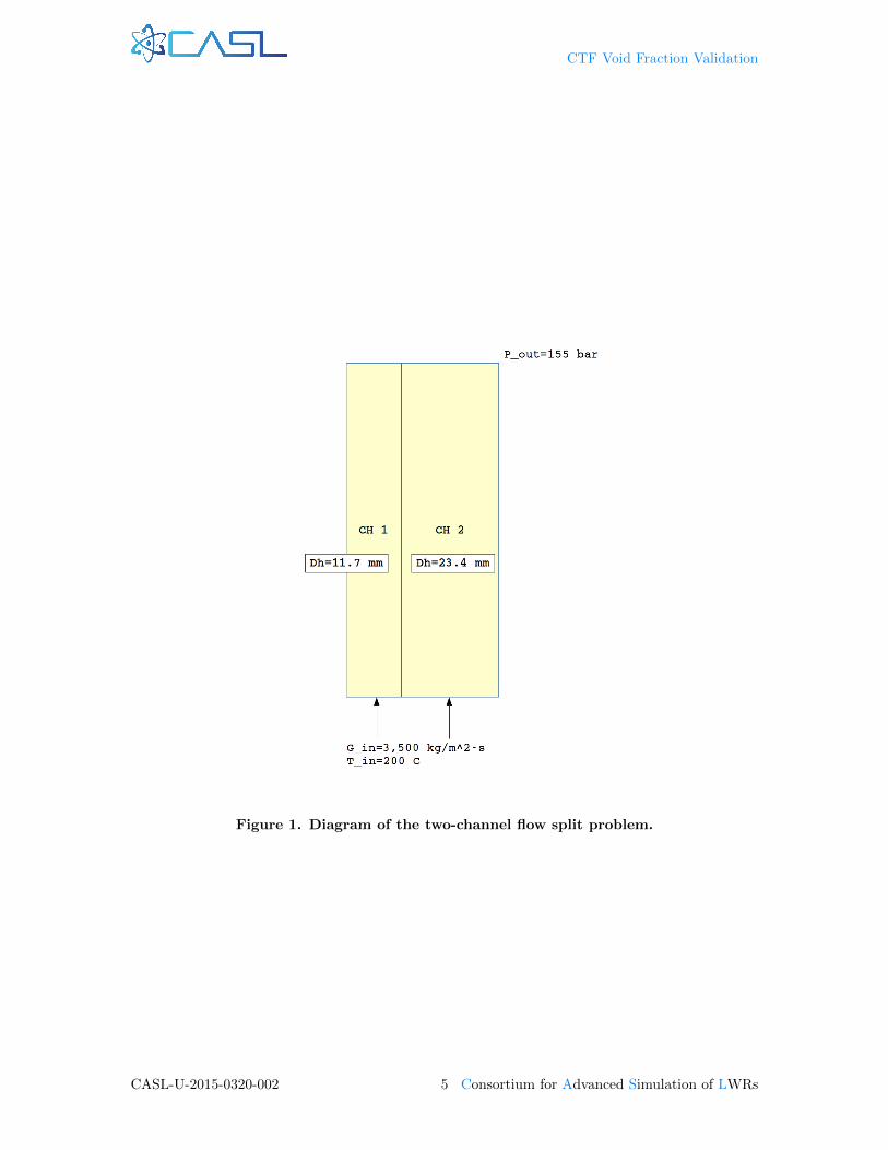
CTF Model Description Channel 2 has a hydraulic diameter that is twice the size of the Channel1 hydraulic diameter. The area and wetted perimeter of Channel 1 are set to values close to thoseexpected of typical pressurized water reactor (PWR) rod-lattice geometry. The outlet pressure is155 bar and inlet mass flux is 3500 kg m−2 s−1. The inlet temperature is set to 200◦C to keep themodel sufficiently subcooled, and the case is unheated. Turbulent mixing and void drift is disabledso that pressure is the only driver for cross-flow. A diagram of this model is shown in Figure 1.The length of the model is set to 10 m to allow the flow to completely redistribute within the CTFsolution space.
The axial mesh is set to different sizes, including 2.54 cm, 5.08 cm, and 10.16 cm; however, it isfound that axial mesh size has no impact on the axial mass flow rate profiles. With the geometrydefined, Equation 12 is used to calculate that the expected outlet mass flow rates in Channels 1 and2.
Discussion of Results The CTF solution includes the axial mass flow rate distribution in eachchannel. The analytical solution only gives us the expected flow rate distribution at the exit.Therefore, we cannot compare the CTF axial flow distribution to the analytical solution, but we canat least guarantee that CTF achieves the correct flow split when mechanical equilibrium is achieved.The mass flux in each channel is normalized before plotting using the following relationship:
Gi,norm =Gi − GG
× 100 (13)
G is the average mass flux between channels, which is equal to the inlet mass flux. Therefore,the normalized mass flux in each channel is zero at the inlet and then re-distributes due to frictionalresistance. Figure 2 shows the CTF-predicted flow distribution in the two-channel system. Thecorrect analytical flow split is shown with the dashed lines.
These results demonstrate that CTF predicts the expected flow split between the two channelsat about 7 m from the inlet.
Consortium for Advanced Simulation of LWRs 4 CASL-U-2015-0320-002
CTF Void Fraction Validation
Figure 1. Diagram of the two-channel flow split problem.
CASL-U-2015-0320-002 5 Consortium for Advanced Simulation of LWRs

CTF Void Fraction Validation
Figure 2. CTF-predicted axial mass flux distribution in two-channel system comparedwith analytical solution.
2.2 Turbulent Mixing Verification
Problem Description The problem consists of two channels connected by a gap. Because theCTF model for turbulent mixing is gradient-driven, it is necessary to make a gradient in eitherenergy or momentum. Because there is no net transfer of mass due to turbulent mixing in singlephase, unheated flows, it is not possible to analyze mass transfer in this case. Forming an analyticalsolution requires us to form and solve the relevant governing equations for the system.
If we choose to look at turbulent mixing of momentum, we will need to set velocity of onechannel higher than the other. The result will be migration of velocity due to pressure-drivendirected cross-flow (due to higher frictional pressure drop in the high velocity channel) as well asturbulent mixing of the momentum. We wish to verify that the turbulent mixing model works asexpected without interference from other effects. We can disable the friction model to stop thepressure-driven directed cross-flow. However, because the axial velocity profile will not be constantin the channel, the convective terms of the momentum equation cannot be eliminated, which requiresa complicated solution of the equations.
The energy equation can be solved much more easily as long as we disable the temperature-dependent density in CTF. With this disabled, the velocity profile will be constant, as the turbulentmixing model for energy does not actually move mass from one channel to another; it captures theeffect of mixing on the migration of energy from one channel to the other.
This problem is a modification of Example 6-1 in Todreas and Kazimi Volume II [5]. The problemin the textbook uses the concept of tracer dyes to demonstrate mixing. In place of looking at mixingof a dye, the mixing of enthalpy is observed in this problem.
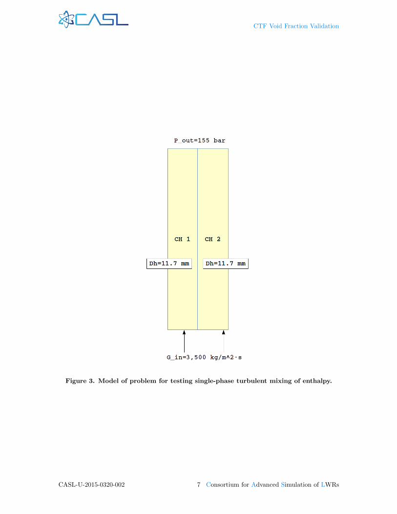
The design of the system is shown in Figure 3. The geometry of the two channels is identical inthis case, which should eliminate any pressure-driven directed cross-flow. Channel geometry is basedon typical PWR rod-lattice geometry. To activate the turbulent-mixing model, the temperature ofone channel is raised 10◦C over the second channel. The “vuq param.txt” file is used to set aconstant liquid density in the system.
Consortium for Advanced Simulation of LWRs 6 CASL-U-2015-0320-002
CTF Void Fraction Validation
Figure 3. Model of problem for testing single-phase turbulent mixing of enthalpy.
CASL-U-2015-0320-002 7 Consortium for Advanced Simulation of LWRs

CTF Void Fraction Validation
For this case, we can set up an energy equation for each channel. The CTF energy equation isas follows:
∂
∂t(αkρkhk) +
∂
∂x(αkρkhkuk) +
∂
∂y(αkρkhkvk) +
∂
∂z(αkρkhkwk) = (14)
ΣNGAPgap=1 q
T ′′′
k,gap + Γ′′′h+ q′′′wk + αk∂P
∂t
The left-hand side terms include: 1) time-change of energy, 2) axial (x) advection of energy,3) lateral (y) advection of energy, and 4) lateral (z) advection of energy. The terms, α, ρ, h, andu, represent the volume fraction, density, enthalpy, and velocity, respectively. The subscript, k,indicates the field; liquid, vapor, or droplet. The right-hand side terms include: 1) turbulent mixingof energy (lateral direction only), 2) the implicit heat transfer, 3) energy entering the volume fromthe wall, and 4) the pressure-work on the volume over time. The term, Γ′′′ represents the volumetricevaporation rate (transfer of mass from the liquid phase to the vapor phase).
We can make the following assumptions about this case:
1. The case is steady-state, eliminating the transient change in energy and the pressure workterm.
2. The case is single-phase, eliminating all k phase subscripts, void fractions, and the mass transferterm.
3. The case is unheated.
4. Because the case is set up so there is no lateral directed cross-flow, only the axial convectiveterm remains.
The simplified equation, with x being the axial direction, becomes
∂
∂x(ρhu) = qT
′′′
y . (15)
The density and velocity can be removed from the derivative because they are constants in thesolution. This is applied directly to our problem of interest by formulating it for each channel in themodel. Substituting the lateral transport of enthalpy due to turbulent mixing (qTy ) with the CTFform of the model yields the following set of equations:
m1d
dxh1 +W ′1→2(h1 − h2) = 0 (16)
m2d
dxh2 −W ′1→2(h1 − h2) = 0 (17)
Each equation is multiplied by the cross-sectional area to convert the velocity to mass flow rateand the volumetric mixing rate to a linear one. The W ′1→2 term represents the mixing rate of energyfrom Channel 1 to Channel 2. It has units of kg m−1 s−1 and is defined as
W ′1→2 = βS12G. (18)
The β term is the turbulent mixing coefficient; it is the “tuning parameter” for the mixing model.Physically, it is a non-dimensional coefficient that represents the ratio of the lateral mass flux dueto mixing to the axial mass flux. The other terms, S12 and G, are the gap width between Channels1 and 2 (in m) and the area-weighted average mass flux between the two channels (in kg m−2 s−1).For this case, we set β to a “typical” value of 0.0035, the gap thickness based on problem geometry(0.003 m), and the mass flux based on problem operating conditions.
Returning to Equations 16 and 17, we can solve the enthalpy distribution in a channel by relatingthe enthalpy in the two channels at any axial level, as follows:
Consortium for Advanced Simulation of LWRs 8 CASL-U-2015-0320-002
CTF Void Fraction Validation
m1h1 + m2h2 = m1h1,in + m2h2,in (19)
Because the mass flow rates in the channels are identical, this term cancels out and we are leftwith a relationship between the enthalpy in Channels 1 and 2 and the known inlet enthalpy boundaryconditions. This is substituted into Equation 16 to develop a first-order, linear, ordinary differentialequation that describes the enthalpy profile in Channel 2:
d
dxh2 +
2W ′1→2
mh2 −
W ′1→2
m(h1,in + h2,in) = 0 (20)
The solution of this equation is
h2 =1
2(h1,in + h2,in) + C exp
(−2W ′1→2
mx
). (21)
Using the inlet enthalpy boundary conditions, the value of the constant, C is determined. Thesame process is repeated for the first channel, leading to the following final solutions for enthalpydistribution in the system due to turbulent mixing.
h1 =1
2(h1,in + h2,in)− 1
2(h2,in − h1,in) exp
(−2W ′1→2
mx
)(22)
h2 =1
2(h1,in + h2,in) +
1
2(h2,in − h1,in) exp
(−2W ′1→2
mx
)(23)
CTF Model Description The CTF input deck is set up from Figure 3. Axial meshing is set to2.54 cm. The gap thickness is set to 0.003 m and its length is set to 0.0126 m, which would resultfrom a PWR lattice with 12.6 mm pitch and 9.5 mm rod outside diameter. The turbulent mixingmodel is set so that a single-phase turbulent-mixing parameter, β, could be set equal to the valueused in the analytical solution. The liquid density is set to a constant value of 700 kg m−3. Note,however, that density does not appear in the analytical solution and, thus, has no impact on theCTF results in terms of turbulent mixing of enthalpy.
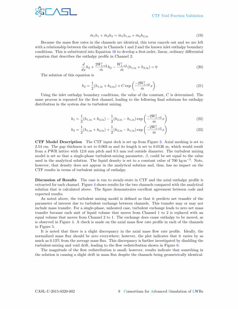
Discussion of Results The case is run to steady-state in CTF and the axial enthalpy profile isextracted for each channel. Figure 4 shows results for the two channels compared with the analyticalsolution that is calculated above. The figure demonstrates excellent agreement between code andexpected results.
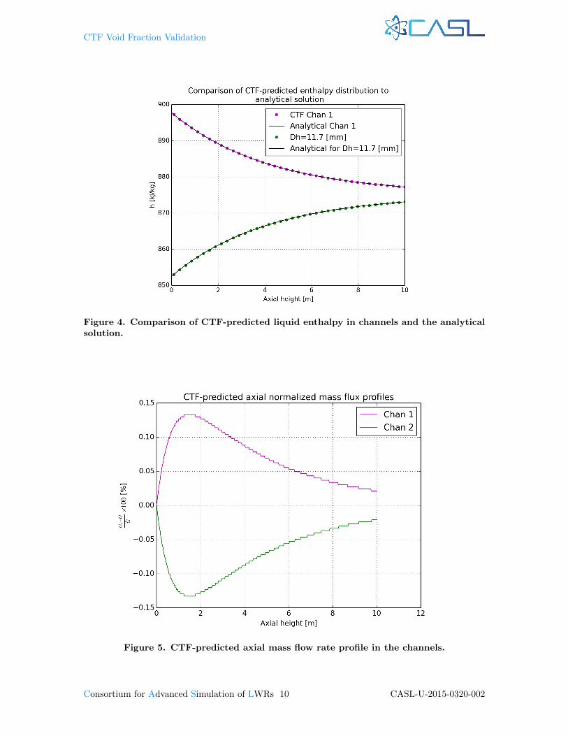
As noted above, the turbulent mixing model is defined so that it predicts net transfer of theparameter of interest due to turbulent exchange between channels. This transfer may or may notinclude mass transfer. For a single-phase, unheated case, turbulent exchange leads to zero net masstransfer because each unit of liquid volume that moves from Channel 1 to 2 is replaced with anequal volume that moves from Channel 2 to 1. The exchange does cause enthalpy to be moved, asis observed in Figure 4. A check is made on the axial mass flow rate profile in each of the channelsin Figure 5.
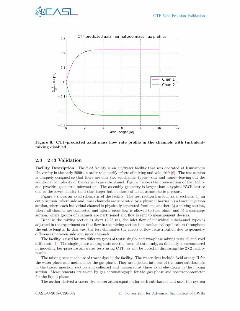
It is noted that there is a slight discrepancy in the axial mass flow rate profile. Ideally, thenormalized mass flux should be zero everywhere; however, the plot indicates that it varies by asmuch as 0.13% from the average mass flux. This discrepancy is further investigated by disabling theturbulent-mixing and void drift, leading to the flow redistribution shown in Figure 6.
The magnitude of the flow redistribution is small; however, results indicate that something inthe solution is causing a slight drift in mass flux despite the channels being geometrically identical.
CASL-U-2015-0320-002 9 Consortium for Advanced Simulation of LWRs
CTF Void Fraction Validation
Figure 4. Comparison of CTF-predicted liquid enthalpy in channels and the analyticalsolution.
Figure 5. CTF-predicted axial mass flow rate profile in the channels.
Consortium for Advanced Simulation of LWRs 10 CASL-U-2015-0320-002
CTF Void Fraction Validation
Figure 6. CTF-predicted axial mass flow rate profile in the channels with turbulent-mixing disabled.
2.3 2×3 Validation
Facility Description The 2×3 facility is an air/water facility that was operated at KumamotoUniversity in the early 2000s in order to quantify effects of mixing and void drift [6]. The test sectionis uniquely designed so that there are only two subchannel types—side and inner—leaving out theadditional complexity of the corner type subchannel. Figure 7 shows the cross-section of the facilityand provides geometric information. The assembly geometry is larger than a typical BWR latticedue to the lower density (and thus larger bubble sizes) of air at atmospheric pressure.
Figure 8 shows an axial schematic of the facility. The test section has four axial sections: 1) anentry section, where side and inner channels are separated by a physical barrier; 2) a tracer injectionsection, where each individual channel is physically separated from one another; 3) a mixing section,where all channel are connected and lateral cross-flow is allowed to take place; and 4) a dischargesection, where groups of channels are partitioned and flow is sent to measurement devices.
Because the mixing section is short (2.25 m), the inlet flow of individual subchannel types isadjusted in the experiment so that flow in the mixing section is in mechanical equilibrium throughoutthe entire length. In this way, the test eliminates the effects of flow redistribution due to geometrydifferences between side and inner channels.
The facility is used for two different types of tests: single- and two-phase mixing tests [6] and voiddrift tests [7]. The single-phase mixing tests are the focus of this study, as difficulty is encounteredin modeling low-pressure air/water tests using CTF, as will be noted in discussing the 2×2 facilityresults.
The mixing tests made use of tracer dyes in the facility. The tracer dyes include Acid orange II forthe water phase and methane for the gas phase. They are injected into one of the inner subchannelsin the tracer injection section and collected and measured at three axial elevations in the mixingsection. Measurements are taken by gas chromatograph for the gas phase and spectrophotometerfor the liquid phase.
The author derived a tracer-dye conservation equation for each subchannel and used this system
CASL-U-2015-0320-002 11 Consortium for Advanced Simulation of LWRs

CTF Void Fraction Validation
Figure 7. Cross-sectional diagram of the 2×3 facility and relevant geometric information(reprinted from M. Sadatomi et al. “Single- and Two-Phase Turbulent Mixing Ratebetween Adjacent Subchanels in a Vertical 2×3 Rod Array Channel”. In InternationalJournal of Multiphase Flow 30 (2004), pp. 481–498.
Figure 8. Side-view schematic of 2×3 facility with visualization of channel partitioningin different axial sections (reprinted from M. Sadatomi et al. “Single- and Two-PhaseTurbulent Mixing Rate between Adjacent Subchanels in a Vertical 2×3 Rod ArrayChannel”. In International Journal of Multiphase Flow 30 (2004), pp. 481–498.
Consortium for Advanced Simulation of LWRs 12 CASL-U-2015-0320-002
CTF Void Fraction Validation
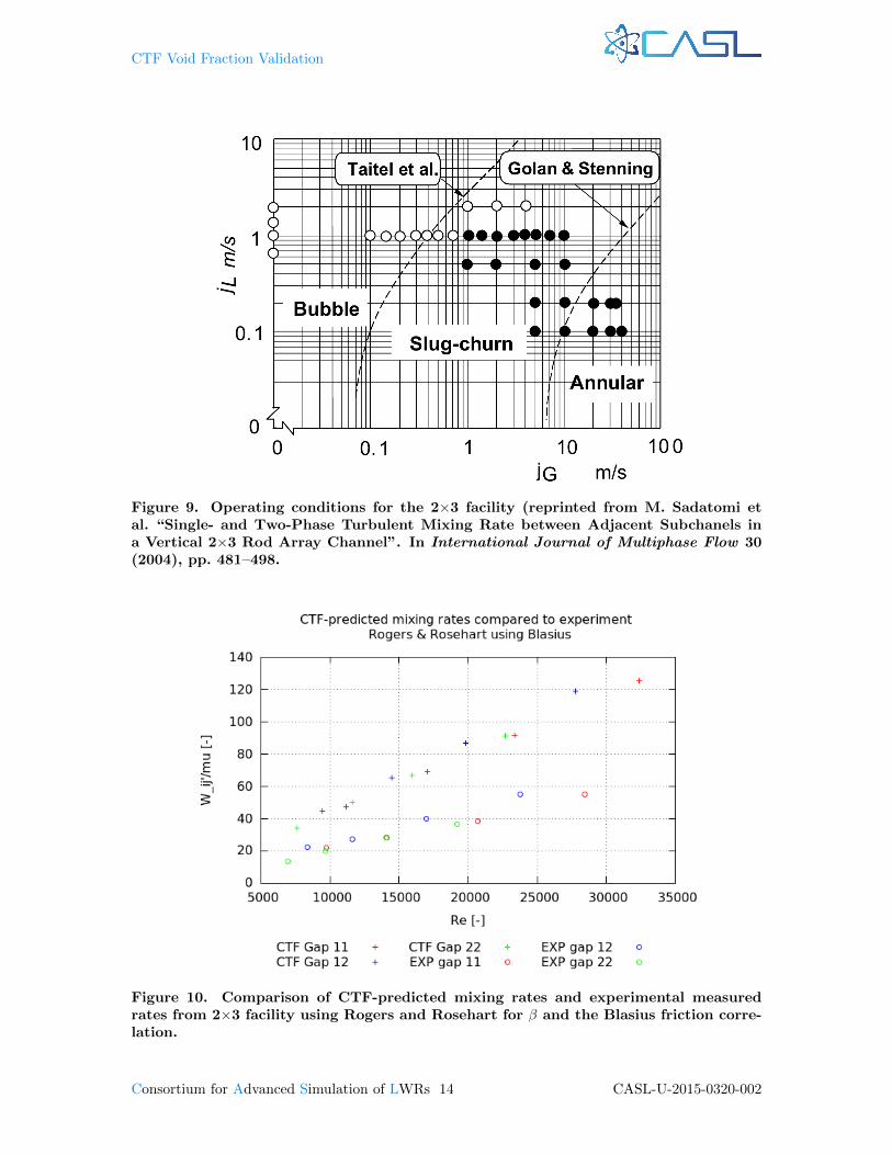
of equations to derive the channel mixing term, w′ij , as a function of tracer dye concentration. Flowconditions for the mixing tests are shown in Figure 9 as liquid and vapor superficial velocity. Onlythe single-phase tests are modeled in this study, which includes four data points. The system is runat room temperature and atmospheric pressure.
CTF Model Description Flow area and wetted perimeter are directly taken from the valuesof Figure 7. An axial mesh size of 2.54 cm is employed, and only the 2.25 m mixing section ismodeled. Because the experimenters set the inlet flow to equal the equilibrium distribution, asimilar approach is used in setting the inlet flow rate in CTF. First, the total injection mass flowrate is determined using the CTF-predicted liquid density, facility flow area, and liquid velocityspecified in the experiment. CTF is run, the outlet flow distribution is obtained, and this is usedas the inlet distribution for the next simulation. This process is repeated until cross-flow ceasesthroughout the facility.
The friction correlation will drive the flow distribution, as shown in Section 2.1. The authorindicates that the Sadatomi friction factor correlation [8] leads to the best agreement with themeasured flow distribution; however, its complexity makes it difficult to enter into CTF withoutsignificant code changes. The author also shows results of the Blasius equation, which seems to alsoperform well. Therefore, the Blasius correlation (Equation 24) is used as a first step in this study;however, the CTF friction correlation (Equation 25), which is a default model in CTF, is also tested.
f = 0.316Re−0.25 (24)
f = 0.204Re−0.2 (25)
The single-phase turbulent mixing coefficient is varied during this study to investigate its impacton mixing results. The inlet temperature is set to 24◦C and the outlet pressure is set to 1.013 25 bar.
Discussion of Results Results are shown as the nondimensional mixing rate, W ′ij/µ, vs. thetwo-channel Reynolds number. The two-channel Reynolds number is calculated as follows:
Reij =ρuijDhij
µ(26)
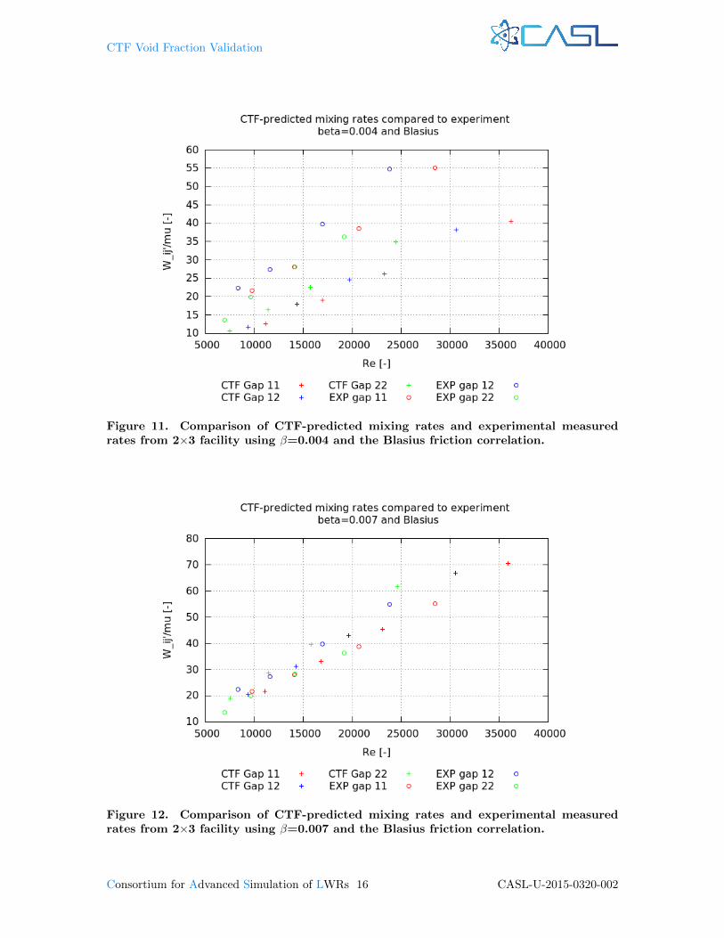
Where the average two-channel velocity, uij , is an area weighted average of the velocities in thetwo adjacent channels, i and j. The hydraulic diameter, Dhij , is the hydraulic diameter of thetwo-channel system, ρ is density, and µ is dynamic viscosity. This is the way in which the authorpresents mixing results. A mixing rate is given for each unique channel connection, which includes:1) inner-to-inner, 2) side-to-inner, and 3) side-to-side for each of the four single phase tests. Figure10 shows the CTF results compared with the experimental results using the Rogers and Rosehartcorrelation [2] to predict single-phase mixing. The Blasius friction factor correlation is used in thiscase.
Two types of data points are shown in the plot: pluses represent the CTF predictions and circlesrepresent the experimental measurements. There are three colors of the data points: red representsthe inner-to-inner connection, green represents the side-to-side connection, and blue represents theside-to-inner connection. Ideally, a “plus” and a “circle” data point should sit in a vertical column;this would mean that the ij Reynolds number of CTF matches the experimental value exactly.Looking at the figure, it is evident this is not the case. The CTF-predicted Reynolds number tendsto be higher than its experimental counterpart in every case.
Likely, there are some differences in steam properties and inlet mass flow rate that lead to thisdiscrepancy. However, it is evident that there is a near-linear trend for nondimensional mixing withrespect to Reynolds number that we can use for comparison. The results of Figure 10 indicatesthat the Rogers and Rosehart correlation over-predicts the mixing rate observed in this facilitysubstantially.
The study is re-run with a user-set, constant single-phase mixing coefficient of 0.004. A mixing-coefficient optimization study done using the CE 5×5 facility [9] (an electrically heated rod bundle
CASL-U-2015-0320-002 13 Consortium for Advanced Simulation of LWRs
CTF Void Fraction Validation
Figure 9. Operating conditions for the 2×3 facility (reprinted from M. Sadatomi etal. “Single- and Two-Phase Turbulent Mixing Rate between Adjacent Subchanels ina Vertical 2×3 Rod Array Channel”. In International Journal of Multiphase Flow 30(2004), pp. 481–498.
Figure 10. Comparison of CTF-predicted mixing rates and experimental measuredrates from 2×3 facility using Rogers and Rosehart for β and the Blasius friction corre-lation.
Consortium for Advanced Simulation of LWRs 14 CASL-U-2015-0320-002

CTF Void Fraction Validation
representative of PWR geometry) found that a value of 0.0044 was optimum for that configuration[10], so 0.004 is considered to be a lower bounding value. Figure 11 shows the results of changingthe mixing coefficient to 0.004.
Results indicate that this mixing coefficient underpredicts the mixing in the facility. As it turnsout, a mixing coefficient of about 0.007 tends to lead to the best agreement, as shown in Figure12. The choice of friction factor correlation has little impact on the predicted mixing rates. Figure13 shows the results using β=0.004 with the friction factor correlation set to the CTF correlationinstead of the Blasius correlation.
It is important to note that the mixing coefficient is simply a tuning parameter that will bedependent on the actual geometry of the facility being modeled. This facility is a square lattice, butthe geometry is much larger than typical PWR or BWR rod-lattice geometry. This study is usefulfor showing that CTF is capable of predicting the correct mixing rate if β is tuned correctly to thefacility. Furthermore, it offers a range of values from which to select the mixing coefficient.
The physical relevance of the mixing rate is not immediately obvious. It is better to observe theimpact of the term on simulation parameters that affect the solution. The CASL Problem 7 challengeproblem (quarter symmetry model of Watts Bar Unit 1) is modeled using a power distribution froma coupled MPACT/CTF solution of the facility. The mixing coefficient is changed from 0.0035 to0.05, with 0.05 being much greater than the value predicted by Rogers and Rosehart. The impactof changing this parameter on local predicted liquid density is shown in Figure 14. The resultsare presented as density in a cell when β is 0.05 minus density in the cell when β is 0.0035. Thiscalculation is made in each of the roughly 500,000 computational cells of the model and presentedin the figure. The results show that differences increase to a maximum at the outlet of the facilityand reach as much as 0.01 g cm−3, which will have a small, but noticeable impact on reactivity inthose locations.
2.4 RPI 2×2 Validation
Facility Description The intended purpose of this experiment (Air/Water Subchannel Measure-ments of the Equilibrium Quality and Mass Flux Distribution in a Rod Bundle) is to investigate thefully developed two-phase flow distribution in a 2×2 rod array test section. The test facility includesa 91.4 cm long unheated 2×2 rod bundle with an air/water mixture as the working fluid. With abundle hydraulic diameter of 23.2 mm, an length-to-diameter ratio of 39 is calculated, leading to anexpected fully-developed flow condition at the bundle outlet.
Four 0.1397 cm thick 314 stainless steel tubes with 2.54 cm outside diameter are used to simulatethe fuel rods. The wall thickness insured a vibration-free environment during the experiment, and alower tie plate provides support for the rods. No spacer grids are used in this experiment. In order torealistically simulate boiling, two different techniques were used to distribute the air into the bundleinlet: a sinter sections technique and a mixing tee technique. An isokinetic sampling approach isused at the bundle outlet to measure liquid and vapor mass flow rates for each unique subchanneltype (i.e., corner, side, and inner). The maximum experimental measurement uncertainty of exitmass flux is estimated to be ±5%. Further details of the facility are summarized in the technicalreport [3] as well as the CTF Validation Manual [4].
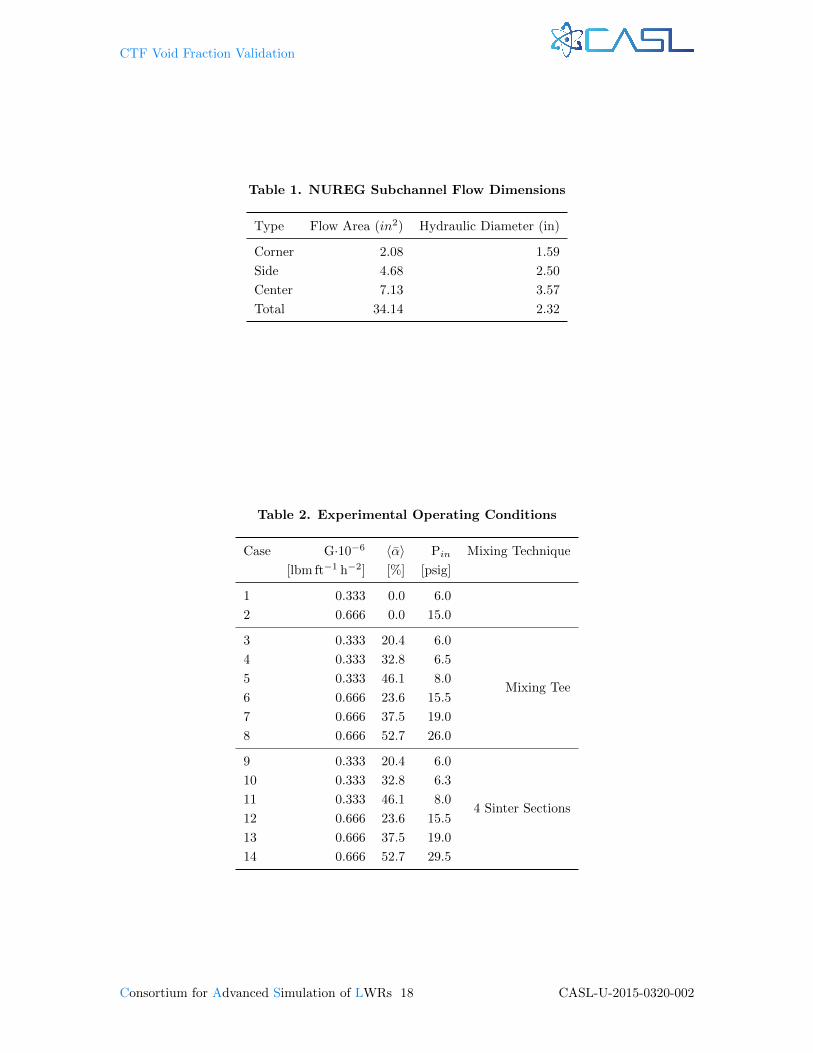
CTF Model Description Table 1 is used to set the channel flow areas in the CTF model. A2.54 cm axial mesh is used. The pressure in Table 2 is used as the outlet pressure boundary condition.The inlet mass flowrate is set from Table 2, and the inlet temperature is set to 21.1◦C, because thetechnical document specifies that the tests were run at room temperature.
Discussion of Results In this step of the validation, we are concerned only with correctly predict-ing the single-phase flow distribution. Therefore, only the two single-phase tests are modeled (Tests1 and 2). The ideal flow distribution is determined similar to how it is in Section 2.1; the momentumequation is used to relate velocity in two individual subchannels, and the mass conservation equationis used to link all channels together. In this case, we have two unique momentum equations and one
CASL-U-2015-0320-002 15 Consortium for Advanced Simulation of LWRs
CTF Void Fraction Validation
Figure 11. Comparison of CTF-predicted mixing rates and experimental measuredrates from 2×3 facility using β=0.004 and the Blasius friction correlation.
Figure 12. Comparison of CTF-predicted mixing rates and experimental measuredrates from 2×3 facility using β=0.007 and the Blasius friction correlation.
Consortium for Advanced Simulation of LWRs 16 CASL-U-2015-0320-002

CTF Void Fraction Validation
Figure 13. Comparison of CTF-predicted mixing rates and experimental measuredrates from 2×3 facility using β=0.007 and the CTF friction correlation.
Figure 14. Variation of local liquid density in CTF simulation of Watts Bar Unit 1when β is changed from 0.0035 to 0.05.
CASL-U-2015-0320-002 17 Consortium for Advanced Simulation of LWRs
CTF Void Fraction Validation
Table 1. NUREG Subchannel Flow Dimensions
Type Flow Area (in2) Hydraulic Diameter (in)
Corner 2.08 1.59
Side 4.68 2.50
Center 7.13 3.57
Total 34.14 2.32
Table 2. Experimental Operating Conditions
Case G·10−6 〈α〉 Pin Mixing Technique
[lbm ft−1 h−2] [%] [psig]
1 0.333 0.0 6.0
2 0.666 0.0 15.0
3 0.333 20.4 6.0
Mixing Tee
4 0.333 32.8 6.5
5 0.333 46.1 8.0
6 0.666 23.6 15.5
7 0.666 37.5 19.0
8 0.666 52.7 26.0
9 0.333 20.4 6.0
4 Sinter Sections
10 0.333 32.8 6.3
11 0.333 46.1 8.0
12 0.666 23.6 15.5
13 0.666 37.5 19.0
14 0.666 52.7 29.5
Consortium for Advanced Simulation of LWRs 18 CASL-U-2015-0320-002

CTF Void Fraction Validation
mass equation with three unknown variables. The coefficients for the CTF friction correlation areused in the momentum equation, leading to an exponent of 2/3 on the ratio of hydraulic diameters.
ucorneruside
=
(DhcornerDhside
)2/3
(27)
ucorneruinner
=
(DhcornerDhinner
)2/3
(28)
mtot = 4ρucornerAcorner + 4ρusideAside + ρuinnerAinner (29)
Solving this system of equations gives an ideal flow split for each individual channel type:
mcorner =mtot
C
(DhcornerDhinner
)2/3(Acorner
Ainner
)(30)
mside =mtot
C
(DhsideDhinner
)2/3(Aside
Ainner
)(31)
minner =mtot
C, where (32)
C = 4
(DhcornerDhinner
)2/3Acorner
Ainner+ 4
(DhsideDhinner
)2/3Aside
Ainner+ 1. (33)
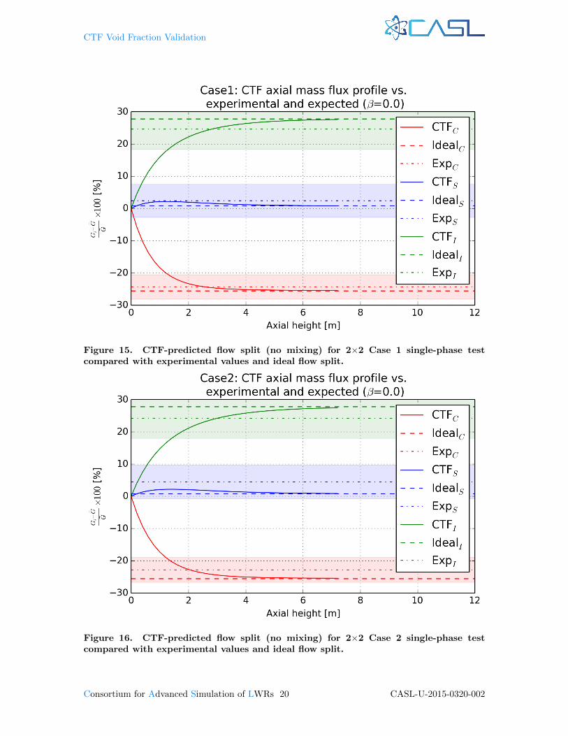
Each single-phase case is first run with turbulent mixing disabled, so as to see that CTF predictsthe correct single-phase flow distribution. Results show that CTF does predict the correct flowdistribution; however, not within the axial length of the test section, which is 1 m. The CTF modelis extended to 7 m to show that the correct flow split is eventually achieved. Figures 15 and 16show the results of running CTF with no turbulent mixing for Case 1 and 2 of the 2×2 facility,respectively.
The channel mass flux results are normalized as shown in Equation 13. The figures show fourimportant pieces of information:
1. The CTF normalized channel mass fluxes are shown for corner, side, and inner type channels(red, blue, and green) using the solid lines,
2. The analytical solution for the flow split (obtained using Equations 30, 31, and 32) is shownwith the three horizontal dashed lines using the same color scheme to denote channel types,
3. The experimental measurements are shown with the dot-dash lines using the same color schemefor denoting channel type, and
4. The shaded regions show the maximum experimental measurement uncertainty for channelmass flux (5%), as quoted in the 2×2 technical report [3].
The figures shows that the trend for flow to migrate into the lower resistance inner channel andout of the higher resistance corner channel is correctly predicted. The CTF channel flows hit theexpected values at about 6 m. The experimental results are not exactly the same as the theoreticalvalues since turbulent mixing drives momentum from the higher velocity inner channel back to thecorner and side channels. However, note that the experimental results are obtained within 1 m oftest section length.
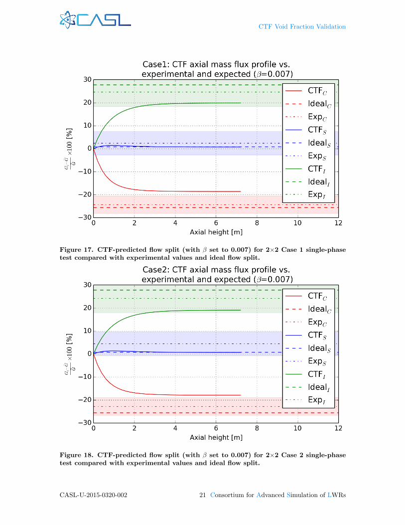
Figures 17 and 18 show the same results with turbulent mixing enabled in CTF and the single-phase turbulent mixing coefficient, β, set to 0.007 (the ideal value discovered in Section 2.2).
Enabling turbulent mixing leads to a new mechanical equilibrium point in CTF. The innerchannel flow does not go as high and corner channel flow does not go as low. The results seem toindicate that the CTF mixing coefficient may be slightly too high for this experimental facility. The
CASL-U-2015-0320-002 19 Consortium for Advanced Simulation of LWRs
CTF Void Fraction Validation
Figure 15. CTF-predicted flow split (no mixing) for 2×2 Case 1 single-phase testcompared with experimental values and ideal flow split.
Figure 16. CTF-predicted flow split (no mixing) for 2×2 Case 2 single-phase testcompared with experimental values and ideal flow split.
Consortium for Advanced Simulation of LWRs 20 CASL-U-2015-0320-002
CTF Void Fraction Validation
Figure 17. CTF-predicted flow split (with β set to 0.007) for 2×2 Case 1 single-phasetest compared with experimental values and ideal flow split.
Figure 18. CTF-predicted flow split (with β set to 0.007) for 2×2 Case 2 single-phasetest compared with experimental values and ideal flow split.
CASL-U-2015-0320-002 21 Consortium for Advanced Simulation of LWRs

CTF Void Fraction Validation
CTF inner channel mass flux is lower than the experimental inner channel measurement and theCTF corner channel mass flux is higher the than the experimental corner measurement. The cornerchannel prediction is just outside of the measurement uncertainty bands.
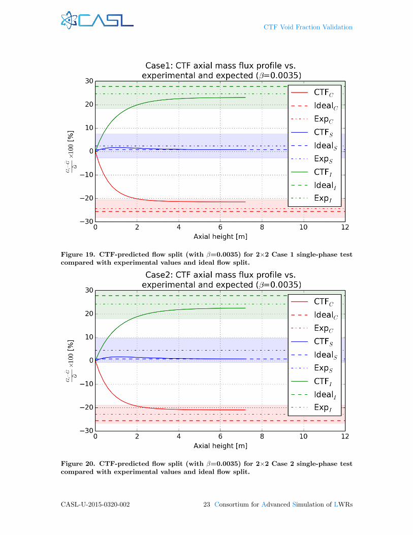
Adjusting the mixing coefficient down to β=0.0035 leads to a more favorable prediction of theflow split, as shown in Figures 19 and 20.
Similar to the cases without mixing, the flow takes about 5–6 m to reach equilibrium distributionin the CTF model. Since Case 2 has a mass flux that is twice that of Case 1, it appears that themagnitude of flow has no significant effect on the distance to reach equilibrium flow distribution.
Consortium for Advanced Simulation of LWRs 22 CASL-U-2015-0320-002
CTF Void Fraction Validation
Figure 19. CTF-predicted flow split (with β=0.0035) for 2×2 Case 1 single-phase testcompared with experimental values and ideal flow split.
Figure 20. CTF-predicted flow split (with β=0.0035) for 2×2 Case 2 single-phase testcompared with experimental values and ideal flow split.
CASL-U-2015-0320-002 23 Consortium for Advanced Simulation of LWRs
CTF Void Fraction Validation
2.5 GE 3×3 Validation
Facility Description The GE 3×3 facility [11] is a classic test for assessing inter-subchannelmixing because mass flux and quality measurements are made for individual subchannel types. A3×3 electrically heated bundle with BWR geometry is used. The axial and radial power profilesare uniform for all of these test cases. The same bundle is used for all the tests. Bundle power,flow rate, and inlet subcooling are varied between different experimental cases. Measurements aremade at the outlet of the facility using an isokinetic sampling approach, similar to the approachused in the 2×2 facility. The estimated maximum error in subchannel flow measurements is ±2%.The authors determined that the error in the exit equilibrium quality measurements were ±0.02.Additional details on the facility can be found in the experiment technical report [11] as well as theCTF Validation Manual [4].
Discussion of Results Because this section of the study is reviewing the ability to predict correctsingle-phase flow distribution, only the four single-phase cases (1B, 1C, 1D, and 1E) are run. Thesecases are not currently included in the CTF Validation Manual [4]. Considering the difficulty CTFexhibited in correctly predicting the flow split for the 2×2 facility, it is prudent to assess the flow-distribution prediction for the GE 3×3 case before analyzing the two-phase void drift cases.
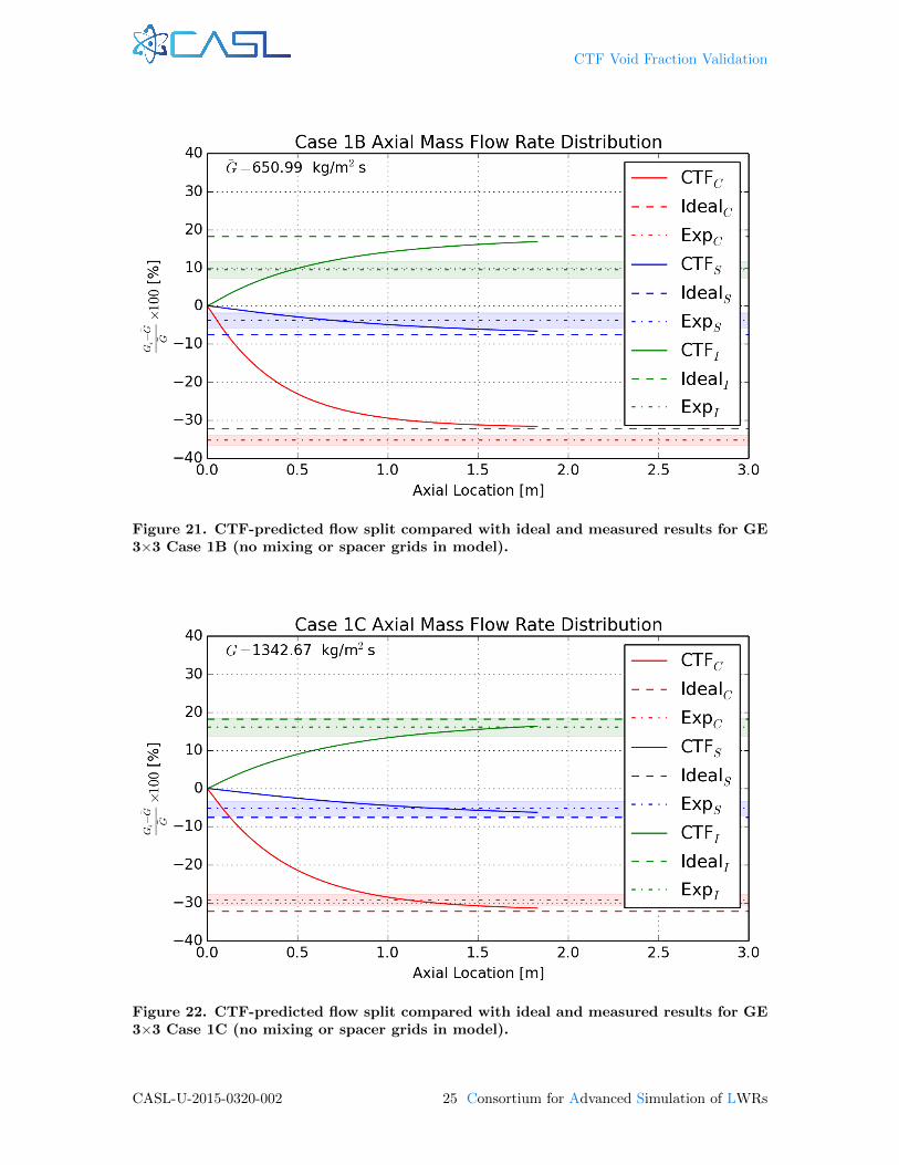
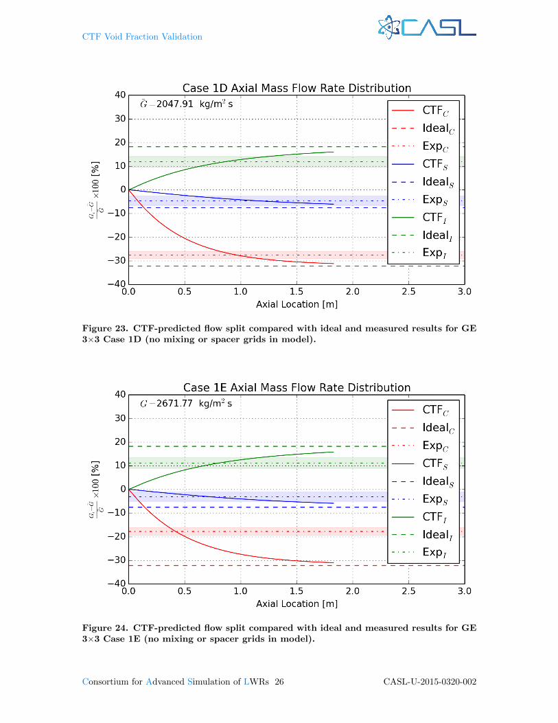
The cases are first run without spacer grids and with turbulent mixing disabled. The idealflow split is calculated using the same approach as Section 2.4. Again, flow results are displayedas normalized values, the ideal flow split is shown with dashed horizontal lines, and the measuredresults are shown with dot-dash lines. The measurement uncertainty is shown as a colored, shadedregion around the measurement line. Figures 21–24 show the result of these predictions for the foursingle-phase cases with no turbulent mixing or form losses.
Similar to the 2×2 facility tests, CTF predicts the correct flow rate distribution; however, itis interesting to note that the equilibrium distribution is achieved in a much shorter length of thefacility. The flow distribution is nearly in equilibrium at the 1.8 m location, which is the exit of thefacility; whereas, the 2×2 facility took nearly 5 m to reach equilibrium.
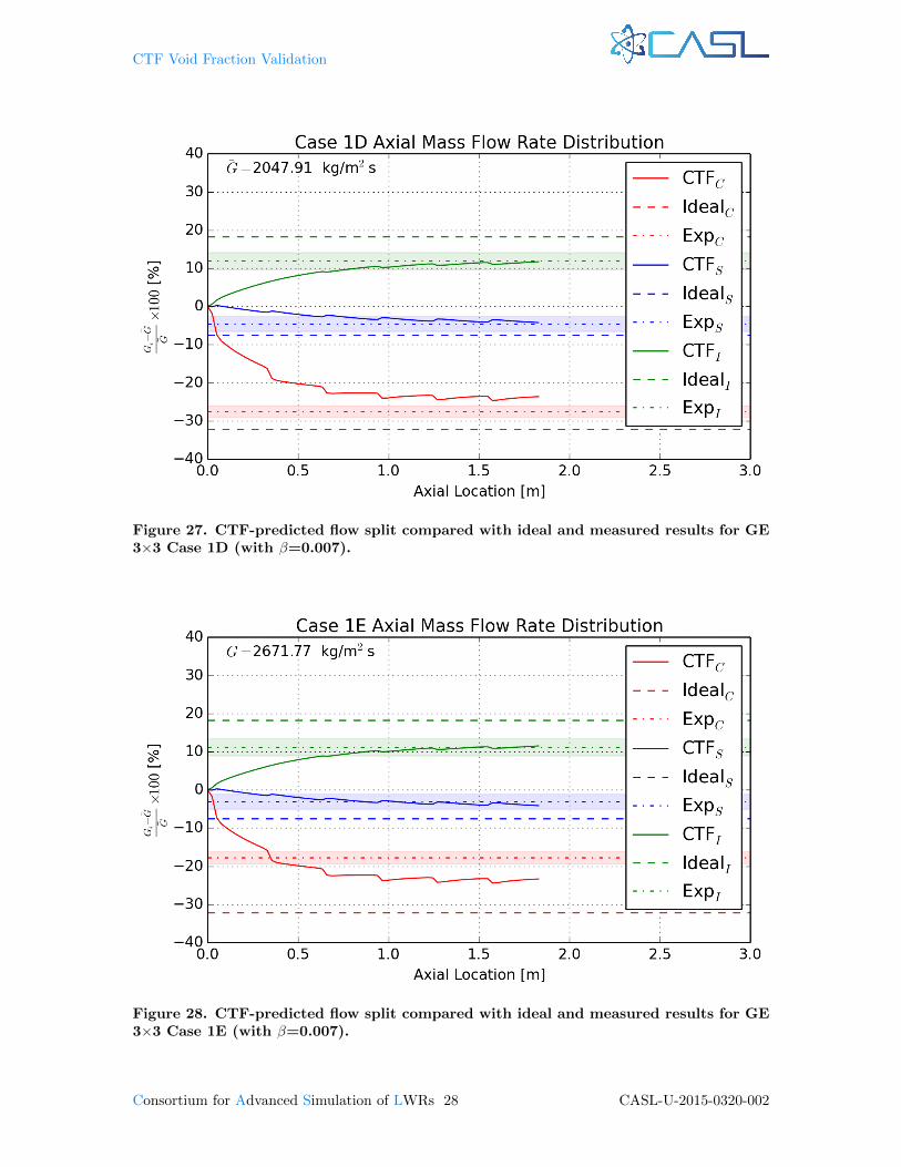
Adding the grids and turbulent mixing produces the results shown in Figures 25–28. The chan-nel mass fluxes are closer to the bundle-average value as a result of the turbulent mixing modelbeing enabled. The addition of the grids results in a “choppy” appearance of the axial mass fluxdistributions. Because the grid form loss coefficient is the same for all channels, the grids have an“equalizing” effect, pushing inner channel flow back into the side and corner channels. The redistri-bution is driven by the fact that the higher-velocity inner channel flow experiences a greater pressureloss than the lower-velocity corner channel at the grid location. The imbalance in flow losses causesflow to migrate from the higher resistance inner channel to the lower resistance corner channel. Theredistribution lasts for a short period downstream of the grid loss and soon reverses so that flowmoves back into the inner channel.
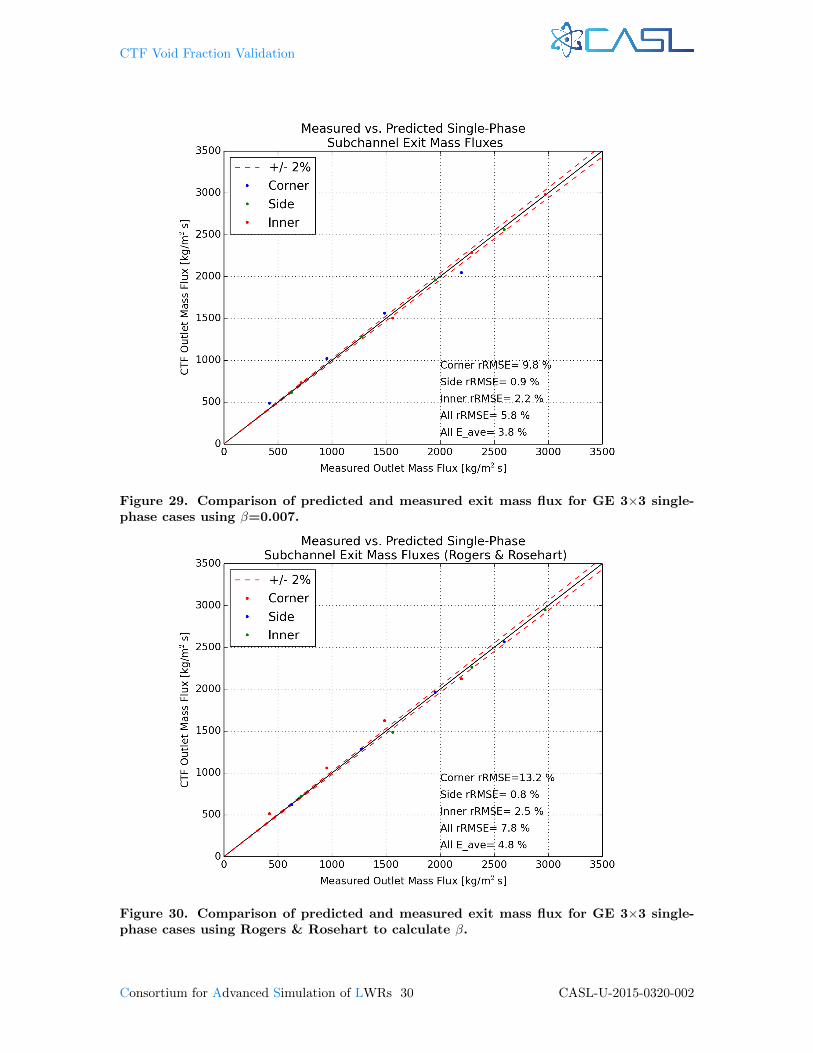
All single-phase predicted outlet mass fluxes are compared with their measured counterparts inFigure 29. Each color represents a unique channel type: red for corner, blue for side, and green forinner. Inner- and side-predicted mas fluxes match experimental values closely, having relative root-mean-square of error (rRMSE) (Equation 34) values that are close to experimental measurementuncertainty. Corner results vary from experimental values by a much larger degree.
rRMSE =
√1
NΣNi=1E
2rel,i, where (34)
Erel =xmeasured − xpredicted
xmeasured(35)
The excellent agreement between CTF and the experiment found in this single-phase study addsmore credibility to the two-phase void drift study performed with this data in the CTF ValidationManual [4]. However, it is noted that the turbulent mixing model in this study is different fromthe one used in the Validation Manual. The original GE 3×3 study was done using the Rogers &Rosehart correlation to calculate the mixing coefficient. This choice is further investigated in thissection and the two-phase void drift modeling section.
Consortium for Advanced Simulation of LWRs 24 CASL-U-2015-0320-002
CTF Void Fraction Validation
Figure 21. CTF-predicted flow split compared with ideal and measured results for GE3×3 Case 1B (no mixing or spacer grids in model).
Figure 22. CTF-predicted flow split compared with ideal and measured results for GE3×3 Case 1C (no mixing or spacer grids in model).
CASL-U-2015-0320-002 25 Consortium for Advanced Simulation of LWRs
CTF Void Fraction Validation
Figure 23. CTF-predicted flow split compared with ideal and measured results for GE3×3 Case 1D (no mixing or spacer grids in model).
Figure 24. CTF-predicted flow split compared with ideal and measured results for GE3×3 Case 1E (no mixing or spacer grids in model).
Consortium for Advanced Simulation of LWRs 26 CASL-U-2015-0320-002

CTF Void Fraction Validation
Figure 25. CTF-predicted flow split compared with ideal and measured results for GE3×3 Case 1B (with β=0.007).
Figure 26. CTF-predicted flow split compared with ideal and measured results for GE3×3 Case 1C (with β=0.007).
CASL-U-2015-0320-002 27 Consortium for Advanced Simulation of LWRs
CTF Void Fraction Validation
Figure 27. CTF-predicted flow split compared with ideal and measured results for GE3×3 Case 1D (with β=0.007).
Figure 28. CTF-predicted flow split compared with ideal and measured results for GE3×3 Case 1E (with β=0.007).
Consortium for Advanced Simulation of LWRs 28 CASL-U-2015-0320-002

CTF Void Fraction Validation
It has been shown in Section 2.2 that the Rogers & Rosehart model tends to exaggerate themixing in the system. The single-phase cases are re-run using the Rogers & Rosehart model for βand measured versus predicted exit mass fluxes are shown in Figure 30. Side and inner results arelargely unaffected, but the corner channel experiences a more significant drop in accuracy. OverallrRMSE increases by two percentage points. The average error (Equation 36) increases from 3.8%to 4.8%.
Erel = ΣNi=1
|xmeasured,i − xpredicted,i|xmeasured,i
× 100 (36)
CASL-U-2015-0320-002 29 Consortium for Advanced Simulation of LWRs
CTF Void Fraction Validation
Figure 29. Comparison of predicted and measured exit mass flux for GE 3×3 single-phase cases using β=0.007.
Figure 30. Comparison of predicted and measured exit mass flux for GE 3×3 single-phase cases using Rogers & Rosehart to calculate β.
Consortium for Advanced Simulation of LWRs 30 CASL-U-2015-0320-002
CTF Void Fraction Validation
3 VOID DRIFT VALIDATION
3.1 RPI 2×2 Validation
The 2×2 facility has been introduced in Section 2.4. The single-phase tests performed in the facilitywere modeled in that section. The facility also includes a series of two-phase tests with inlet voidranging from 20 to 50%. Several attempts are made to model the two phase tests of this facility;however, limited success is achieved when attempting to run the models at the atmospheric pressurespecified in the test specification.
It is not possible to model the facility using the non-condensable gas model in CTF becauseCTF assumes that the non-condensable gas mixture fills the vapor phase. At atmospheric pressureand room temperature, any vapor in the model condenses away, forcing the non-condensable gasvoid fraction to zero. Therefore, it is necessary to model the facility as a two-phase, steam/watermixture. It is possible to shut off the evaporation/condensation term in CTF so that the vaporphase behaves as a non-condensable gas.
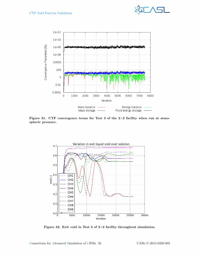
The first attempt at modeling the facility involves using the experimental pressure as the outletboundary condition in CTF. Running a two-phase mixture at this pressure leads to large gradientsin the steam and liquid fluid properties, which makes it more difficult for the code to converge on asteady-state solution. An example of the code convergence terms is shown in Figure 31. As indicatedin the figure, all convergence terms simply oscillate for the duration of the simulation.
It is important to look at actual simulation results behavior throughout the simulation. The exitvapor void is checked in the nine channels of the model at each iteration. They are plotted in Figure32. The void almost settles on a constant value in each of the channels. The corner channel void(Channels 1, 3, and 9) seem to be experiencing a slow oscillation. However, note that there is nosymmetry in the results. The corner channel void (Channels 1, 3, 7, and 9) should all be identical inthe converged solution. Likewise, the side channel void (Channels 2, 4, 6, and 8) should be identical.
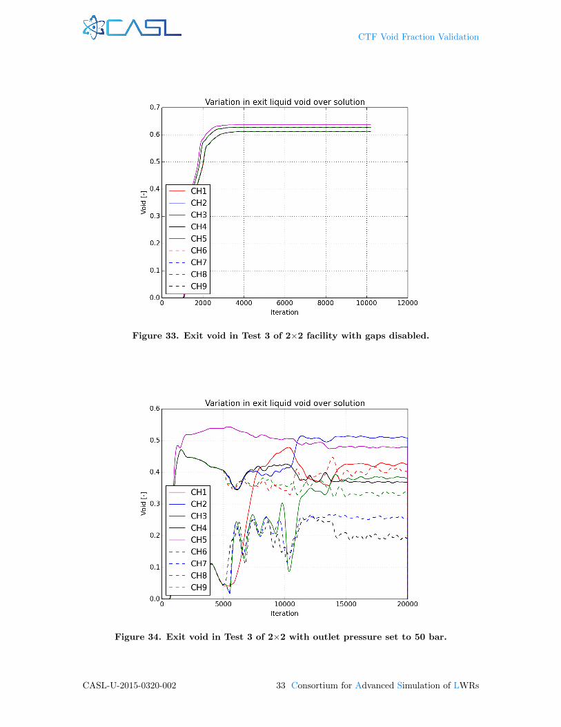
The case is rerun with the gaps disabled (a collection of nine isolated subchannels) as a sanitycheck. Results are shown in Figure 33. Here, we see a smooth change in void over the simulation.The simulation only takes about 4,000 iteration to converge. All side-channel voids are identical,and all corner-channel voids are identical, as expected.
It is found that increasing pressure in the system is an effective means of improving code conver-gence. However, large pressure increases are required to allow all cases to converge. The test casepressure is first increased to 50 bar; the inlet enthalpy is increased to keep the mixture two-phase.Figure 34 shows the result. The void distribution is chaotic in time and space. However, observethat increasing the mixture enthalpy, and thus the bundle void, allows the code to converge (Figure35).
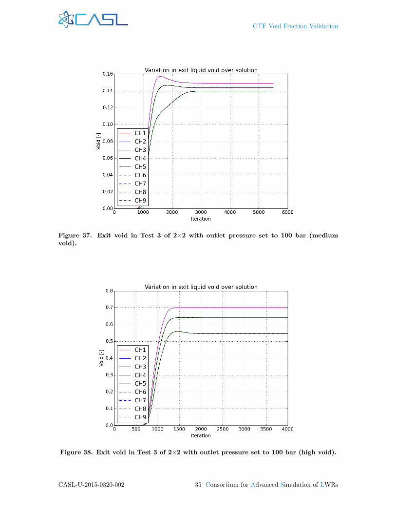
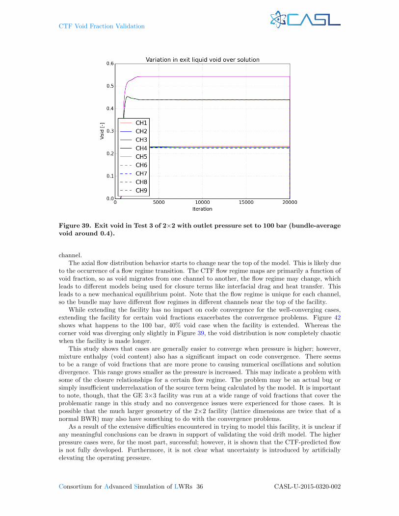
Increasing the pressure further to 100 bar allows the code to converge for a wider range of mixtureenthalpy. Figure 36 shows a low void case, Figure 37 shows a higher void case, and Figure 38 showsa very high void case. All cases converge nicely. However, the code still has some trouble convergingin a certain range of void fractions. Figure 39 demonstrates that the corner channel voids start todiverge slightly at a bundle-average void of around 0.4.
The previous study involving these tests, which is documented in the CTF Validation document[4], used this artificially elevated operating pressure of 100 bar to allow the cases to converge.Running at this much higher pressure increases the vapor-to-liquid density ratio to 0.08. In reality,this ratio was about 0.002 in the experiments. Furthermore, the inlet Reynolds number increasesfrom roughly 40,000 to about 120,000 because of changing fluid properties. These changes introducean unknown amount of uncertainty into the results. Furthermore, as noted in Section 2.4, CTF doesnot predict the equilibrium flow distribution by the outlet of this facility.
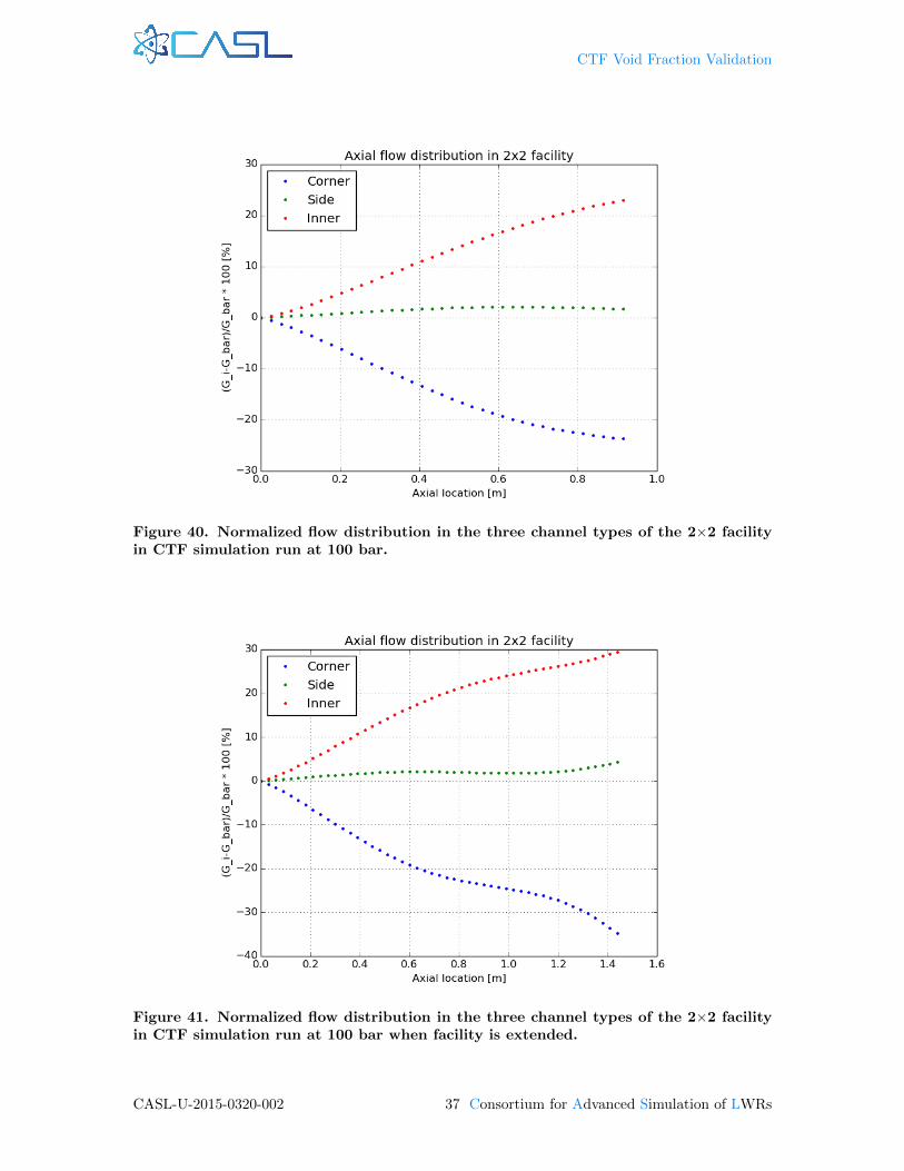
It is useful to investigate the effect of lengthening the CTF model. Figure 40 shows the normalizedmass flux distribution in the three channel types along the length of the test section. It looks asthough the flow distribution at the outlet has almost reached its equilibrium value; however, whenthe test section is extended slightly in Figure 41, it is seen that the converged flow distributionhas not actually reached equilibrium; axial mass fluxes begin to move apart from one another nearthe end of the bundle, with mass flux increasing in the inside channel and decreasing in the corner
CASL-U-2015-0320-002 31 Consortium for Advanced Simulation of LWRs
CTF Void Fraction Validation
Figure 31. CTF convergence terms for Test 3 of the 2×2 facility when run at atmo-spheric pressure.
Figure 32. Exit void in Test 3 of 2×2 facility throughout simulation.
Consortium for Advanced Simulation of LWRs 32 CASL-U-2015-0320-002
CTF Void Fraction Validation
Figure 33. Exit void in Test 3 of 2×2 facility with gaps disabled.
Figure 34. Exit void in Test 3 of 2×2 with outlet pressure set to 50 bar.
CASL-U-2015-0320-002 33 Consortium for Advanced Simulation of LWRs

CTF Void Fraction Validation
Figure 35. Exit void in Test 3 of 2×2 with outlet pressure set to 50 bar and mixtureenthalpy increased.
Figure 36. Exit void in Test 3 of 2×2 with outlet pressure set to 100 bar (low void).
Consortium for Advanced Simulation of LWRs 34 CASL-U-2015-0320-002
CTF Void Fraction Validation
Figure 37. Exit void in Test 3 of 2×2 with outlet pressure set to 100 bar (mediumvoid).
Figure 38. Exit void in Test 3 of 2×2 with outlet pressure set to 100 bar (high void).
CASL-U-2015-0320-002 35 Consortium for Advanced Simulation of LWRs
CTF Void Fraction Validation
Figure 39. Exit void in Test 3 of 2×2 with outlet pressure set to 100 bar (bundle-averagevoid around 0.4).
channel.The axial flow distribution behavior starts to change near the top of the model. This is likely due
to the occurrence of a flow regime transition. The CTF flow regime maps are primarily a function ofvoid fraction, so as void migrates from one channel to another, the flow regime may change, whichleads to different models being used for closure terms like interfacial drag and heat transfer. Thisleads to a new mechanical equilibrium point. Note that the flow regime is unique for each channel,so the bundle may have different flow regimes in different channels near the top of the facility.
While extending the facility has no impact on code convergence for the well-converging cases,extending the facility for certain void fractions exacerbates the convergence problems. Figure 42shows what happens to the 100 bar, 40% void case when the facility is extended. Whereas thecorner void was diverging only slightly in Figure 39, the void distribution is now completely chaoticwhen the facility is made longer.
This study shows that cases are generally easier to converge when pressure is higher; however,mixture enthalpy (void content) also has a significant impact on code convergence. There seemsto be a range of void fractions that are more prone to causing numerical oscillations and solutiondivergence. This range grows smaller as the pressure is increased. This may indicate a problem withsome of the closure relationships for a certain flow regime. The problem may be an actual bug orsimply insufficient underrelaxation of the source term being calculated by the model. It is importantto note, though, that the GE 3×3 facility was run at a wide range of void fractions that cover theproblematic range in this study and no convergence issues were experienced for those cases. It ispossible that the much larger geometry of the 2×2 facility (lattice dimensions are twice that of anormal BWR) may also have something to do with the convergence problems.
As a result of the extensive difficulties encountered in trying to model this facility, it is unclear ifany meaningful conclusions can be drawn in support of validating the void drift model. The higherpressure cases were, for the most part, successful; however, it is shown that the CTF-predicted flowis not fully developed. Furthermore, it is not clear what uncertainty is introduced by artificiallyelevating the operating pressure.
Consortium for Advanced Simulation of LWRs 36 CASL-U-2015-0320-002
CTF Void Fraction Validation
Figure 40. Normalized flow distribution in the three channel types of the 2×2 facilityin CTF simulation run at 100 bar.
Figure 41. Normalized flow distribution in the three channel types of the 2×2 facilityin CTF simulation run at 100 bar when facility is extended.
CASL-U-2015-0320-002 37 Consortium for Advanced Simulation of LWRs

CTF Void Fraction Validation
Figure 42. 2×2 Test 3 run at 100 bar and 40% void when facility length is extended.
3.2 GE 3×3 Validation
The 3×3 facility was introduced in Section 2.5. The single-phase tests were modeled in that section,and it was demonstrated that CTF predicts the correct flow distribution for single-phase flow. Thetwo-phase tests were modeled previously in the CTF Validation Manual [4]. This study expands onthe previous validation work by including all test cases (some test cases were not included in theoriginal validation work) and using the optimal mixing coefficient of 0.007 along with the effect ofswitching from Rogers & Rosehart. Additionally, this study observes behavior of the axial mass fluxdistribution predicted by CTF rather than only the predicted outlet mass flux value.
CTF Model Description The base CTF model is described in Section 2.5. The geometry of alltests is the same, so only the boundary conditions need to be modified between runs. The processof generating the input decks, running them, and processing results is scripted so that sensitivitystudies and automated testing may be performed easily. This study includes several perturbationsof modeling choices of interest:
• The mixing model is changed between a constant of 0.007 and the Rogers & Rosehart model.
• A case is run with void drift disabled.
• A case is run with no grids for observing axial flow behavior.
Discussion of Results A comparison of the measured and predicted exit equilibrium qualities isprovided in Figure 43 for the base case model, which uses the void drift model with Ka set to 1.4,the turbulent mixing model with βsp set to 0.007, and ΘM set to 5.0. Figure 43 shows that mostpredicted exit qualities fall within experimental uncertainty. However, the values that seem to varyfurthest from measured results are qualities in the corner type subchannel. Root-mean-square of theerror (RMSE) (Equation 37) values for the three subchannel types are shown directly in the figure.
RMSE =
√1
NΣNi=1(xctf,i − xm,i)2 (37)
Consortium for Advanced Simulation of LWRs 38 CASL-U-2015-0320-002
CTF Void Fraction Validation
We see that, on average, the corner channel quality prediction error is about double the innerand side type channel prediction error. Furthermore, quality in the corner channels is typically over-predicted by CTF. The side and inner type exit qualities, however, generally match the experimentalvalues within the measurement uncertainty.
If the void drift model is disabled, comparisons with experimental data become much worse.Figure 44 shows the exit equilibrium quality compared with experimental measurements with thevoid drift model disabled. Corner channel root-mean-square of error (RMSE) increases from 0.044to 0.121 and inner channel RMSE increases from 0.012 to 0.019 for exit quality.
In addition to the exit equilibrium quality, the authors also measured the exit mass flux of eachindividual subchannel. Results for the two-phase experiments are shown in Figure 45. The rRMSEfor the two-phase experiments are larger than for the single-phase results shown in Figure 29. Thecorner is still the most poorly predicted of all channel types. Figure 46 shows the exit mass flux forthe two-phase cases when void drift is disabled. The accuracy of both corner and inner channel typepredictions degrades sharply. Similarly, mass flux rRMSE more than doubles for the corner channeltype when the void drift model is disabled.
The original GE 3×3 study used the Rogers & Rosehart correlation to set the single-phase mixingcoefficient. The results are repeated here for all experiments in Figures 47 and 48 for mass flux andquality. Prediction of both measured quantities improves when using Rogers & Rosehart over theconstant β value of 0.007. Results indicate there is almost no difference in accuracy of the resultsbetween using the Rogers & Rosehart correlation to calculate single-phase mixing coefficient or theconstant value of 0.007.
The axial mass flux distribution of each channel type is also investigated. It is discovered thatthe distributions are complicated, so the spacer grids are removed for the sake of clarifying two-phaseand flow-regime dependant trends. The turbulent-mixing and void drift models are enabled, withthe single-phase mixing coefficient being set to 0.007 with the Beus two-phase-mixing multiplier setto 5.0. The following plots show the normalized mass flux in each channel type, calculated as localmass flux minus bundle average mass flux and divided by bundle average mass flux. The measurednormalized mass fluxes are shown with horizontal dashed lines. The measured value is only availableat the outlet. Different colored lines are used to denote different channel types; red for corner, bluefor side, and green for inner.
The plots also include the flow regime, denoted with colored regions in the plot; SP stands forsingle-phase, SB for small bubble, SL for slug, CH for churn, and AN for annular. The flow regimesoften change at different axial locations in different channel types. The gray shaded regions showthe length of this transition region. For example, the green “SB” region means that all channeltypes are in the small bubble flow regime. When the gray region begins, it means at least one of thechannel types has transitioned to slug flow, but at least one channel type is still in small bubble.When the gray region ends, it means that all channels are in slug. The flow quality is shown foreach channel type using dot-dashed lines, which corresponds to a secondary y-axis.
The high-flow, low-power cases, 2C1 and 2C2, are shown in Figures 49 and 50. The figures showthat the corner mass flux tends to decrease and inner mass flux tends to increase until the flowquality starts to increase. At this point, the void drift effect begins to draw the normalized massfluxes back toward zero. Test 2C2 has lower subcooling, so this effect starts sooner in the bundle.In Case 2C2, there is a “notch” in the axial mass flux profile for the corner channel. It is found thatthis is due to entrainment starting by running a case with the droplet field disabled.
The axial flow behavior is fairly smooth in the “C”-series cases compared with higher powercases and lower flow cases. Test 2G1 has the power doubled compared with the 2C1 and 2C2 cases.Its flow distribution is shown in Figure 51. Because of high subcooling, the exit flow quality is stillonly about 10%, but the flow distributions look more chaotic starting at about the 0.8 m mark. Theflow distribution appears to begin changing in the slug flow regime and transition to churn.
The “D”-series tests have the highest power-to-flow ratio. Test 2D3 makes it into the annularflow regime as a result. Its axial flow distribution is shown in Figure 52. Flow quality goes as highas almost 40%. The flow distribution experiences a significant trend reversal at about 1.5 m, as thechannels transition into the annular flow regime. Again, there is a “notch” in the corner channelmass flux distribution due to the start of entrainment.
CASL-U-2015-0320-002 39 Consortium for Advanced Simulation of LWRs
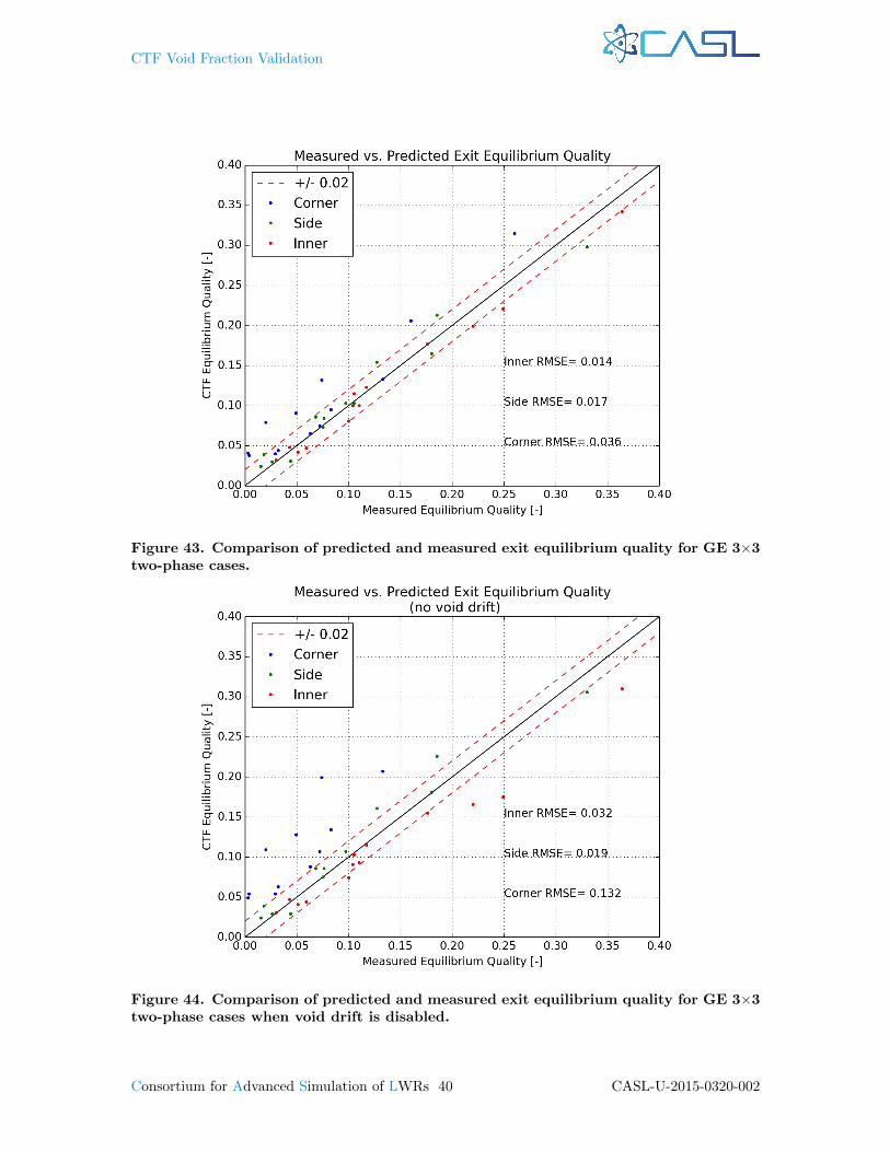
CTF Void Fraction Validation
Figure 43. Comparison of predicted and measured exit equilibrium quality for GE 3×3two-phase cases.
Figure 44. Comparison of predicted and measured exit equilibrium quality for GE 3×3two-phase cases when void drift is disabled.
Consortium for Advanced Simulation of LWRs 40 CASL-U-2015-0320-002
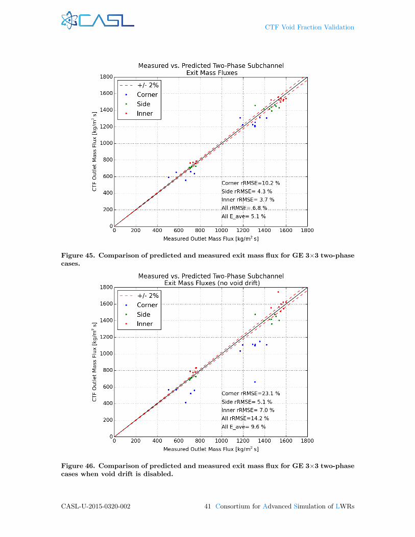
CTF Void Fraction Validation
Figure 45. Comparison of predicted and measured exit mass flux for GE 3×3 two-phasecases.
Figure 46. Comparison of predicted and measured exit mass flux for GE 3×3 two-phasecases when void drift is disabled.
CASL-U-2015-0320-002 41 Consortium for Advanced Simulation of LWRs

CTF Void Fraction Validation
Figure 47. Comparison of predicted and measured exit mass flux for GE 3×3 two-phasecases using Rogers & Rosehart.
Figure 48. Comparison of predicted and measured exit quality for GE 3×3 two-phasecases using Rogers & Rosehart.
Consortium for Advanced Simulation of LWRs 42 CASL-U-2015-0320-002

CTF Void Fraction Validation
The overall trend seems for flow to migrate from the corner channel to the side and inner channelswhen flow is low void. At the start of bulk boiling, this trend reverses, causing channel flow to staythe same or move back to the average. The transition to the annular flow regime causes a secondreversal, making flow migrate out of the corner channel and back into the inner and side channelsdue to a change in constitutive models.
CASL-U-2015-0320-002 43 Consortium for Advanced Simulation of LWRs

CTF Void Fraction Validation
Figure 49. GE 3×3 Test 2C1 CTF-predicted axial flow distribution and flow qualitydistribution compared with experimental measurement.
Figure 50. GE 3×3 Test 2C2 CTF-predicted axial flow distribution and flow qualitydistribution compared with experimental measurement.
Consortium for Advanced Simulation of LWRs 44 CASL-U-2015-0320-002
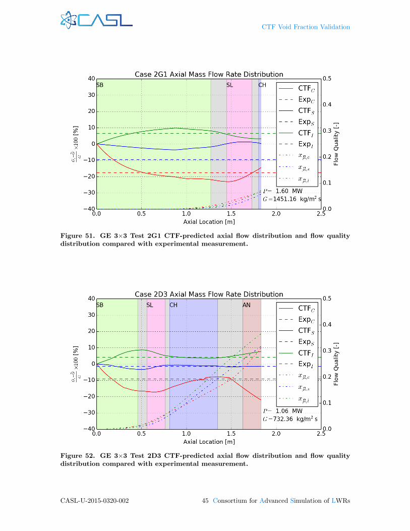
CTF Void Fraction Validation
Figure 51. GE 3×3 Test 2G1 CTF-predicted axial flow distribution and flow qualitydistribution compared with experimental measurement.
Figure 52. GE 3×3 Test 2D3 CTF-predicted axial flow distribution and flow qualitydistribution compared with experimental measurement.
CASL-U-2015-0320-002 45 Consortium for Advanced Simulation of LWRs

CTF Void Fraction Validation
3.3 BFBT 8×8 Validation
Facility Description The BFBT tests are organized into phases and exercises as described in theBFBT specification [12].
• Phase I: Void Distribution Benchmark
– Exercise 1: Steady-state subchannel grade benchmark
– Exercise 2: Steady-state microscopic grade benchmark
– Exercise 3: Transient microscopic grade benchmark
– Exercise 4: Uncertainty analysis of the void distribution benchmark
• Phase II: Critical Power Benchmark
– Exercise 0: Steady-state pressure drop benchmark
– Exercise 1: Steady-state critical power benchmark
– Exercise 2: Transient benchmark
The CTF Validation document [4] includes tests from Phase II, Exercise 0. This validation studyexpands on the BFBT tests included in the CTF validation matrix by modeling Phase I, Exercise1. For this validation study, 16 tests are modeled. Table 3 shows the tests and their operatingconditions that are modeled as part of this study.
The assembly type refers to the placement of heater rods, guide tubes, the water rod, and powerconfigurations. Figures 53 and 54 show the geometry and rod configuration for Assembly Types0-1, 0-2, and 0-3. All of these tests have a uniform axial and radial heating. The only differencebetween the assembly types is that some heater rods are shut off in Assembly Types 0-2 and 0-3.Figure 55 shows the geometry and power configuration for Assembly Types 1, 2, and 3. Only testsof Assembly Type 1 are modeled in this study. Assembly Type 1 has a cosine power shape, whichis shown in Table 4. All other assembly types modeled in this study have a uniform axial powershape. Assembly Types 1 and 4 have non-uniform radial power distributions. The Assembly Type 1radial power distribution is shown in Figure 56, and the Assembly Type 4 radial power distributionis shown in Figure 57.
Finally, Figure 58 shows the rod configuration and power distribution for Assembly Types 4,C2A, C2B, and C3. Only tests of Assembly Type 4 are included in this study. Assembly Type 4replaces the four central rods with a large water rod.
Void measurements were made in the facility using two approaches: 1) an x-ray densitometerwas used at several axial locations, and 2) a CT scanner was used to obtain a fine-mesh voiddistribution measurement 50 mm above the end of heated length. The CT scanner measurementsare used for comparison with CTF in this study. Figure 59 shows a schematic of where differentvoid measurements were made in the facility.
The CT scanner worked by sweeping over the bundle at a fixed axial plane to obtain voidmeasurements in small “pixels” as small as 0.3×0.3 mm. The refined measurements have beenused for CFD validation work, but the measurements were also post-processed to create a set ofsubchannel-averaged void measurements for comparison with subchannel codes. The measurementswere made several times for the same operating conditions and were time-averaged to avoid theeffects of two-phase flow oscillations.
The BFBT specification [12] states that the subchannel accuracy is estimated to be 3% and thebundle average void is estimated to be 2% (as will be shown when analyzing symmetry of the results,the measurement error is likely much higher than this).
CTF Model Figure 60 shows the flow area and wetted perimeter for the channels in the CTFmodel for Assembly Types 0-1, 0-2, 0-3, and 1. It also shows the channel indexing scheme employedin the model. Note that the center channel is indexed as Channel 81. For the Assembly Type 4,Channel 81 is simply removed from the model along with the four surrounding rods. A large waterrod is positioned in their place and the flow areas are modified as shown in Figure 61.
Consortium for Advanced Simulation of LWRs 46 CASL-U-2015-0320-002
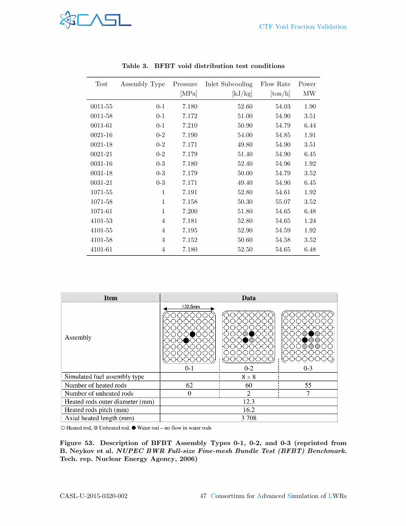
CTF Void Fraction Validation
Table 3. BFBT void distribution test conditions
Test Assembly Type Pressure Inlet Subcooling Flow Rate Power
[MPa] [kJ/kg] [ton/h] MW
0011-55 0-1 7.180 52.60 54.03 1.90
0011-58 0-1 7.172 51.00 54.90 3.51
0011-61 0-1 7.210 50.90 54.79 6.44
0021-16 0-2 7.190 54.00 54.85 1.91
0021-18 0-2 7.171 49.80 54.90 3.51
0021-21 0-2 7.179 51.40 54.90 6.45
0031-16 0-3 7.180 52.40 54.96 1.92
0031-18 0-3 7.179 50.00 54.79 3.52
0031-21 0-3 7.171 49.40 54.90 6.45
1071-55 1 7.191 52.80 54.61 1.92
1071-58 1 7.158 50.30 55.07 3.52
1071-61 1 7.200 51.80 54.65 6.48
4101-53 4 7.181 52.80 54.65 1.24
4101-55 4 7.195 52.90 54.59 1.92
4101-58 4 7.152 50.60 54.58 3.52
4101-61 4 7.180 52.50 54.65 6.48
Figure 53. Description of BFBT Assembly Types 0-1, 0-2, and 0-3 (reprinted fromB. Neykov et al. NUPEC BWR Full-size Fine-mesh Bundle Test (BFBT) Benchmark.Tech. rep. Nuclear Energy Agency, 2006)
CASL-U-2015-0320-002 47 Consortium for Advanced Simulation of LWRs
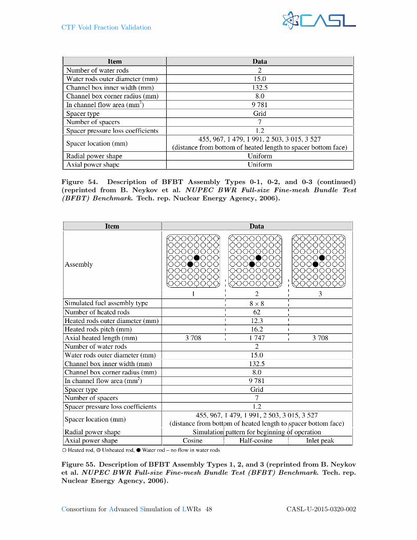
CTF Void Fraction Validation
Figure 54. Description of BFBT Assembly Types 0-1, 0-2, and 0-3 (continued)(reprinted from B. Neykov et al. NUPEC BWR Full-size Fine-mesh Bundle Test(BFBT) Benchmark. Tech. rep. Nuclear Energy Agency, 2006).
Figure 55. Description of BFBT Assembly Types 1, 2, and 3 (reprinted from B. Neykovet al. NUPEC BWR Full-size Fine-mesh Bundle Test (BFBT) Benchmark. Tech. rep.Nuclear Energy Agency, 2006).
Consortium for Advanced Simulation of LWRs 48 CASL-U-2015-0320-002
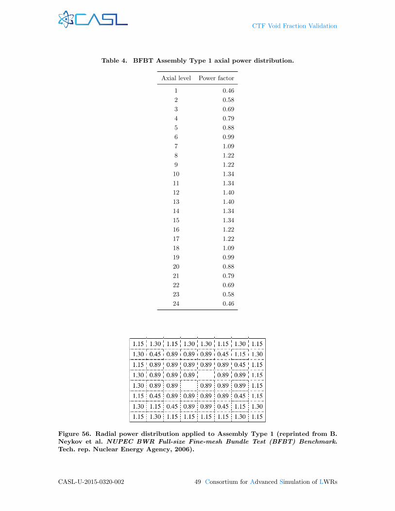
CTF Void Fraction Validation
Table 4. BFBT Assembly Type 1 axial power distribution.
Axial level Power factor
1 0.46
2 0.58
3 0.69
4 0.79
5 0.88
6 0.99
7 1.09
8 1.22
9 1.22
10 1.34
11 1.34
12 1.40
13 1.40
14 1.34
15 1.34
16 1.22
17 1.22
18 1.09
19 0.99
20 0.88
21 0.79
22 0.69
23 0.58
24 0.46
Figure 56. Radial power distribution applied to Assembly Type 1 (reprinted from B.Neykov et al. NUPEC BWR Full-size Fine-mesh Bundle Test (BFBT) Benchmark.Tech. rep. Nuclear Energy Agency, 2006).
CASL-U-2015-0320-002 49 Consortium for Advanced Simulation of LWRs

CTF Void Fraction Validation
Figure 57. Radial power distribution applied to Assembly Type 4 (reprinted from B.Neykov et al. NUPEC BWR Full-size Fine-mesh Bundle Test (BFBT) Benchmark.Tech. rep. Nuclear Energy Agency, 2006).
Figure 58. Description of BFBT Assembly Type 4 (reprinted from B. Neykov et al. NU-PEC BWR Full-size Fine-mesh Bundle Test (BFBT) Benchmark. Tech. rep. NuclearEnergy Agency, 2006).
Consortium for Advanced Simulation of LWRs 50 CASL-U-2015-0320-002
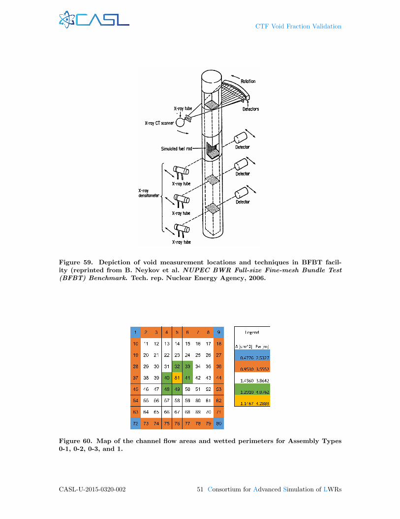
CTF Void Fraction Validation
Figure 59. Depiction of void measurement locations and techniques in BFBT facil-ity (reprinted from B. Neykov et al. NUPEC BWR Full-size Fine-mesh Bundle Test(BFBT) Benchmark. Tech. rep. Nuclear Energy Agency, 2006.
Figure 60. Map of the channel flow areas and wetted perimeters for Assembly Types0-1, 0-2, 0-3, and 1.
CASL-U-2015-0320-002 51 Consortium for Advanced Simulation of LWRs

CTF Void Fraction Validation
Figure 61. Map of the channel flow areas and wetted perimeters for Assembly Type 4.
Spacer grid locations are provided in Figures 53, 54, 55, and 58. These are ferrule-type spacerswith circular tubes (ferrules) to guide each heated rod as well as the central water rod. An exampleof this type of grid is shown in Figure 62.
The loss coefficients for this type of spacer grid are calculated using the approach of Shiralkarand Radcliffe [13]. Details of the calculation are shown in [14]. Figure 63 shows the radial losscoefficient distribution in the bundle.
The CTF friction correlation is used [2] along with a single-phase mixing coefficient of 0.007 anda Beus two-phase multiplier, ΘM , of 5.0. The cases are run once with the droplet field enabled andonce with the droplet field disabled to test the effect. When the droplet field is disabled, it meansthat there is no entrainment or de-entrainment and the interfacial drag and heat transfer betweendroplets and vapor is eliminated in the solution. It is discovered that the droplet field causes minorconvergence problems and degrades the accuracy of results for all channel types, so the majority ofresults are presented with the droplet field disabled.
The axial mesh is set up so that the height of a spacer grid occupies one full level. The averageaxial mesh cell height is 3.635 cm. Only heater rods are explicitly modeled; unheated objects, suchas guide tubes and the fuel canister, are not modeled, as they have no impact on the solution in asteady-state solve. Furthermore, the power is set as a heat flux boundary condition, which disablesthe internal rod temperature solution.
Discussion of Results The process of running the simulations, extracting data from CTF outputfiles, and creating plots is scripted for automated regeneration of analysis results. Most of the casesrun by CTF converged to within tolerance. Convergence is checked by checking a collection ofengineering parameters of interest:
1. Global energy balance (energy into the system minus energy out),
2. Energy movement between fields,
3. Global mass balance (mass into the system minus mass out),
4. Mass movement between fields due to evaporation/condensation,
5. Fluid energy storage between time steps,
6. Solid energy storage between time steps, and
7. Mass storage between time steps.
Consortium for Advanced Simulation of LWRs 52 CASL-U-2015-0320-002
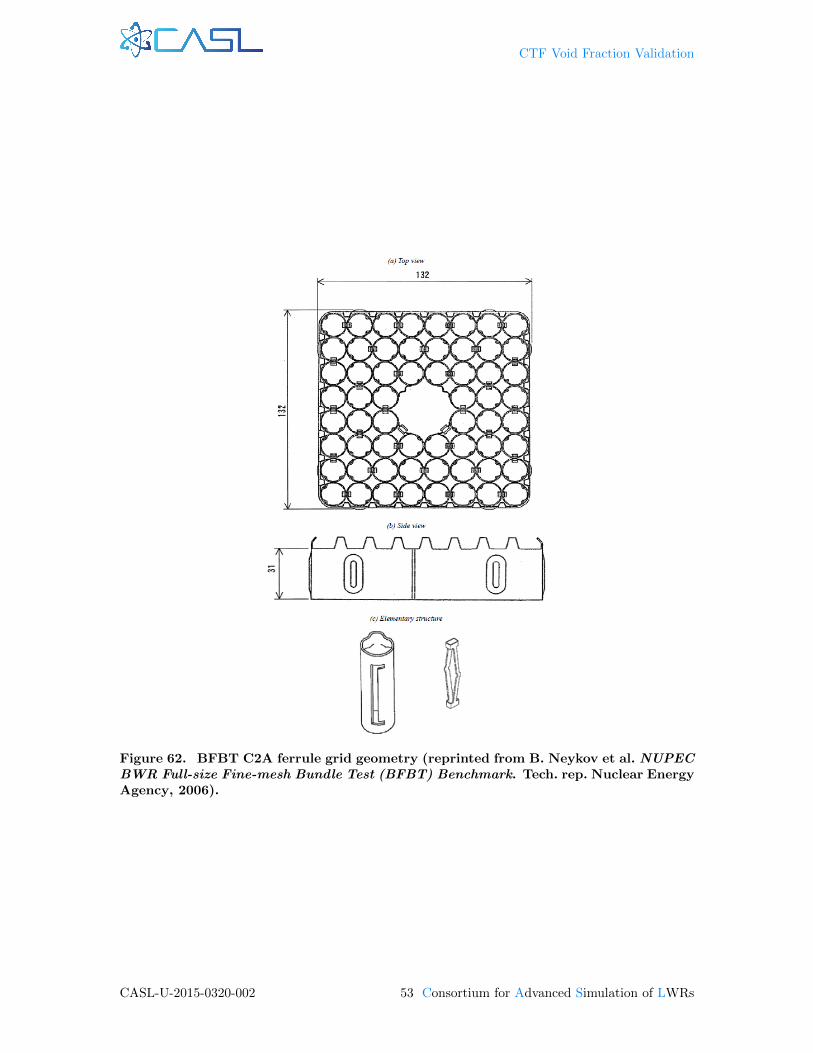
CTF Void Fraction Validation
Figure 62. BFBT C2A ferrule grid geometry (reprinted from B. Neykov et al. NUPECBWR Full-size Fine-mesh Bundle Test (BFBT) Benchmark. Tech. rep. Nuclear EnergyAgency, 2006).
CASL-U-2015-0320-002 53 Consortium for Advanced Simulation of LWRs

CTF Void Fraction Validation
72 73 74 75 76 77 78 79 80
63 64 65 66 67 68 69 70 71
54 55 56 57 58 59 60 61 62
45 46 47 48 49 50 51 52 53
37 38 39 40 41 42 43 44
28 29 30 31 32 33 34 35 36
19 20 21 22 23 24 25 26 27
10 11 12 13 14 15 16 17 18
1 2 3 4 5 6 7 8 9
Legend:k=1.348 k=1.606 k=1.304 k=0.778k=1.278 k=1.222 k=0.748 k=0.856k=0.926
Figure 63. Map of channels in BFBT cases with loss coefficient for each channel ascalculated by Shiralkar and Radcliffe (B. Shiralkar and D. Radcliffe. An Experimentaland Analytical Study of the Synthesis of Grid Spacer Loss Coefficients. Tech. rep.NEDE-13181. General Electric, 1971).
All of these terms need to drop below a user-set tolerance. The tolerance for these cases isinitially set to the same tolerance used for PWR cases. All cases except for two—0011-61 and 1071-61—are able to converge to steady-state within the PWR convergence criteria when the dropletfield is disabled. When the droplet field is enabled, two additional cases fail to converge to withinthe PWR tolerance—1071-55 and 4101-61. It is expected that CTF will not be able to convergeas tightly for high-void cases, where there is a great deal of mass and energy transfer happeningbetween the phases, as it does for single-phase cases. The fact that the rod conduction equationsolution is explicitly coupled to the fluid energy solution, rather than an implicit coupling, likelyworsens this problem.
The tolerance of the non-converging cases has to be increased to 1% for the energy balances, themass balances, and the mass storage (Items 1, 2, 3, 4, and 5 from the list above). The tolerance forfluid energy storage has to be increased to 2%. The tolerances used for PWR cases are 0.01% forItems 1, 2, 3, and 4 and 0.5% for Items 5, 6, and 7. Item 6, the solid energy storage, has no impacton these simulations because the solids (heater rods, water rods, and fuel canister) are not modeledin CTF for these cases.
As a first step, CTF-predicted bundle average void at the outlet and thermal equilibrium qualityis compared with the experimental results. Both values are area-weighted during the averagingprocess. The comparison of CTF-predicted and measured bundle average outlet void is shown inFigure 64 and the comparison of CTF-predicted and measured bundle average thermal equilibriumquality is shown in Figure 65.
There is a tendency for CTF to consistently overpredict the bundle-average void. The overpre-diction is more severe for the cases with lower amounts of void (about 40%). At outlet void ofabout 80%, the prediction almost matches the experimental values. If the same amount of energy isentering the CTF model as is entering the experimental facility, the mixture enthalpy at the outletshould be identical to the experiment (barring steam table differences), which means the void con-tent should also be equal. It is possible the experimental facility loses heat along the axial length,
Consortium for Advanced Simulation of LWRs 54 CASL-U-2015-0320-002
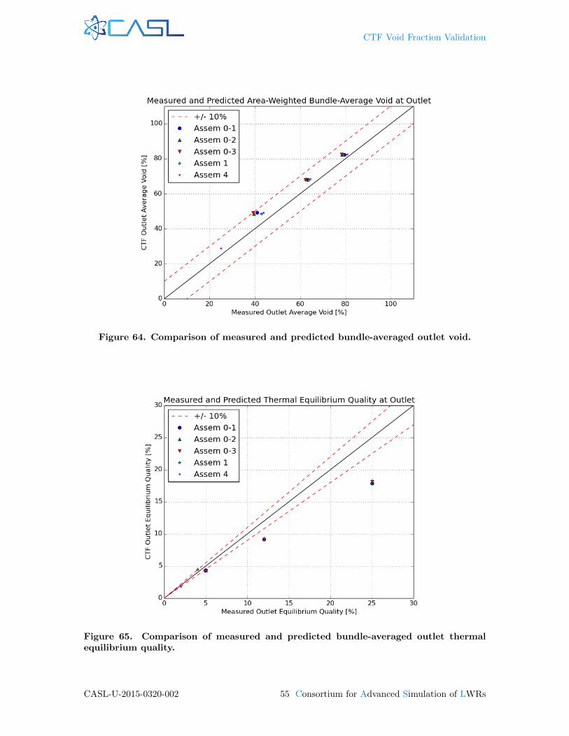
CTF Void Fraction Validation
Figure 64. Comparison of measured and predicted bundle-averaged outlet void.
Figure 65. Comparison of measured and predicted bundle-averaged outlet thermalequilibrium quality.
CASL-U-2015-0320-002 55 Consortium for Advanced Simulation of LWRs

CTF Void Fraction Validation
which therefore leads to a lower amount of void at the outlet compared with the perfectly adiabaticCTF simulation.
The behavior observed in Figure 65 is anomalous. Considering that the average outlet void pre-dicted by CTF is consistently overestimated, one would expect that the exit thermal equilibriumquality would also be higher than experiment. The thermal equilibrium quality is a function ofmixture enthalpy, which should be higher in the CTF model because of higher amounts of void.However, the comparison of predicted and measured quality indicates that CTF predicts substan-tially lower quality than the experiment at the outlet. The experiment specification is not clear onhow exit flow and enthalpy were measured or how thermal equilibrium was calculated, so furtherinvestigation of this inconsistency is not possible.
Before comparing specific channel outlet void measurements to CTF predictions, it is usefulto check the symmetry of the experimental data. To do this, the measurements are grouped intocategories set by the channel types, which are
1. corner channel,
2. side channel,
3. normal inner channel, and
4. inner channel touching unheated element.
The grouping is not perfect, as none of the assembly types are eighth-core symmetric, and thechannels touching unheated elements have different flow areas and wetted perimeters and touch dif-ferent numbers of heated rods. Regardless, the selected categorization leads to a simpler organizationof the data, and we should expect variation in corner and side channels due to assembly asymmetryto be minimal because of their large distance from the asymmetric center of the assembly. The checkis done only for Assembly Types 0-1 and 0-2. Assembly Type 0-3 contains a large unheated sectionin the bundle that is asymmetric and close to the boundary rods, which we expect to lead to moresignificant asymmetry effects. Assembly Types 1 and 4 have non-uniform radial power distributions,which invalidate the selected data categorization.
Figures 66 and 67 give the mean void for each category as well as the spread of the data. Thex-axis contains the four categories. The y-axis is the local subchannel void measurement. The dotgives the mean void for that category, and the error bars give the minimum and maximum voidmeasurement for that category. The horizontal black lines give the bundle-average void at the outletfor each test in the figure. There are three tests shown in each figure (one figure per assembly type).
A few conclusions are drawn from the figures. First, the corner channel measurements tendto have the least scatter in measurement data, whereas the side channels tend to have the largestamount of scatter. Measurements for a given channel type tend to vary by as much as 10–20%, whichsuggests that the measurement uncertainty may be larger than the 3% value quoted in the BFBTspecification. Another observation is that the void drift phenomena becomes evident when comparingmean void to bundle-average void for all experiments. The corner and side voids are typically belowthe bundle-average value, whereas the inner channel void is typically above the bundle-average void.As expected, the channels that touch unheated elements often have the lowest void. The void inunheated channels is lowest for Assembly Type 0-2, which has two heater rods disabled in the centerof the assembly. It is additionally noted that this trend is more exaggerated for test cases withlower total void content. As total void content increases, the outlet void distribution tends to bemore uniform. Although conclusions on data symmetry cannot be drawn for the remaining assemblytypes, similar plots are shown in Figures 68–70 to demonstrate the void drift trend for the otherassembly types.
Figure 71 gives an overview of the measured versus predicted subchannel void measurementsfor all tests. The data is grouped by assembly type, so multiple experiments are included in eachdataset. The data shows that there is an overprediction of void; data is frequently over the +10% linebut never falls below the -10% line. Also, the data appears to form into horizontal “stripes.” This isdue to the asymmetric behavior and spread of the experimental data compared with the symmetricbehavior of the CTF predictions. The RMSE of all data is 7.95% compared with experimental data.
Consortium for Advanced Simulation of LWRs 56 CASL-U-2015-0320-002
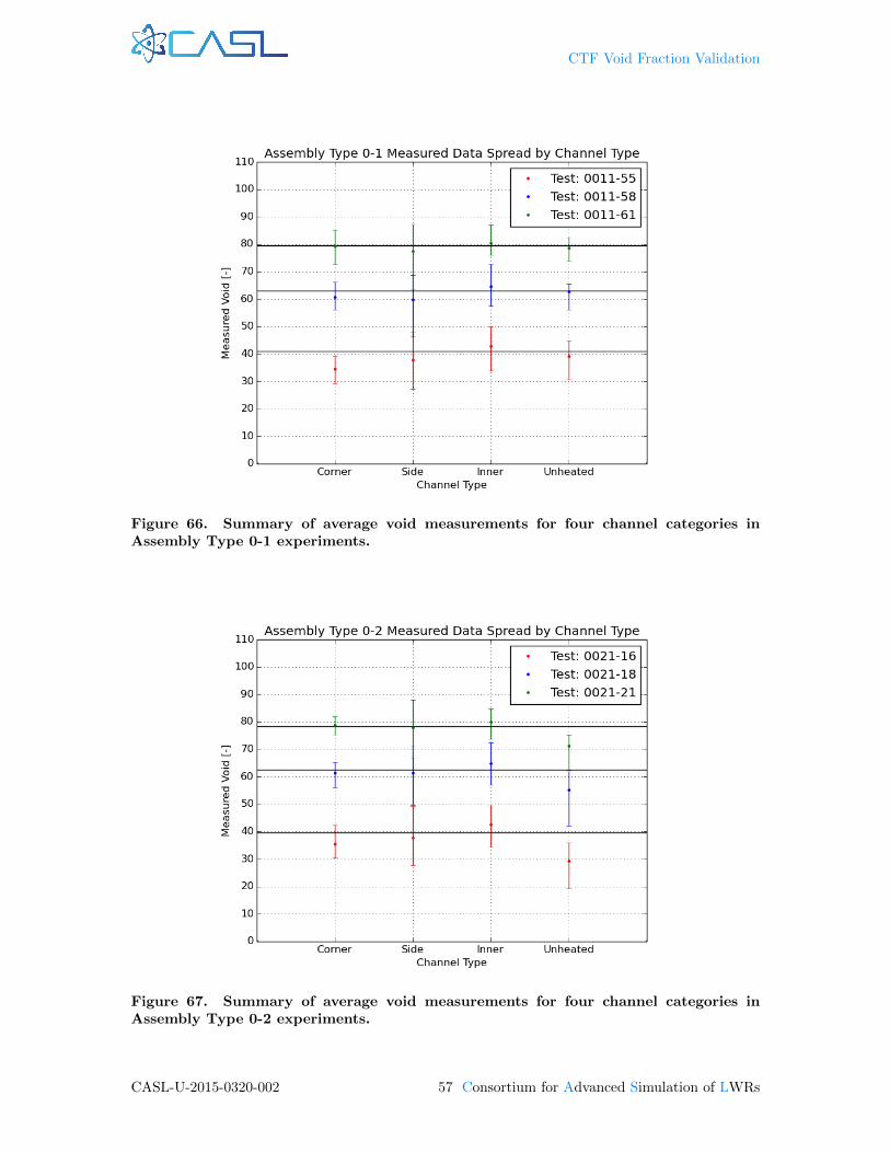
CTF Void Fraction Validation
Figure 66. Summary of average void measurements for four channel categories inAssembly Type 0-1 experiments.
Figure 67. Summary of average void measurements for four channel categories inAssembly Type 0-2 experiments.
CASL-U-2015-0320-002 57 Consortium for Advanced Simulation of LWRs
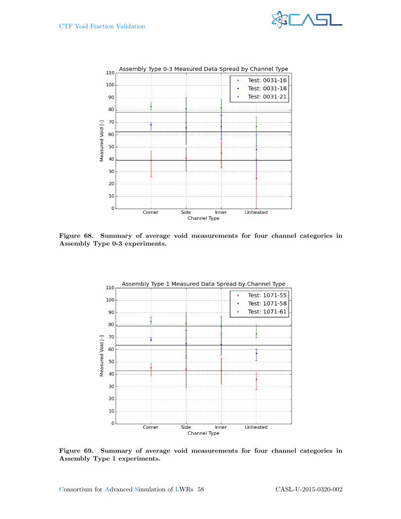
CTF Void Fraction Validation
Figure 68. Summary of average void measurements for four channel categories inAssembly Type 0-3 experiments.
Figure 69. Summary of average void measurements for four channel categories inAssembly Type 1 experiments.
Consortium for Advanced Simulation of LWRs 58 CASL-U-2015-0320-002
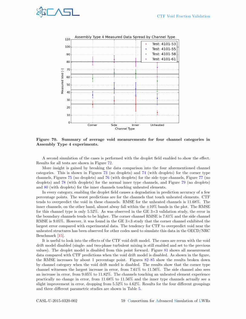
CTF Void Fraction Validation
Figure 70. Summary of average void measurements for four channel categories inAssembly Type 4 experiments.
A second simulation of the cases is performed with the droplet field enabled to show the effect.Results for all tests are shown in Figure 72.
More insight is gained by breaking the data comparison into the four aforementioned channelcategories. This is shown in Figures 73 (no droplets) and 74 (with droplets) for the corner typechannels, Figures 75 (no droplets) and 76 (with droplets) for the side type channels, Figure 77 (nodroplets) and 78 (with droplets) for the normal inner type channels, and Figure 79 (no droplets)and 80 (with droplets) for the inner channels touching unheated elements.
In every category, enabling the droplet field causes a degradation in prediction accuracy of a fewpercentage points. The worst predictions are for the channels that touch unheated elements. CTFtends to overpredict the void in these channels. RMSE for the unheated channels is 11.68%. Theinner channels, on the other hand, almost alway fall within the ±10% bands in the plot. The RMSEfor this channel type is only 5.52%. As was observed in the GE 3×3 validation study, the error inthe boundary channels tends to be higher. The corner channel RMSE is 7.61% and the side channelRMSE is 9.05%. However, it was found in the GE 3×3 study that the corner channel exhibited thelargest error compared with experimental data. The tendency for CTF to overpredict void near theunheated structures has been observed for other codes used to simulate this data in the OECD/NRCBenchmark [15].
It is useful to look into the effects of the CTF void drift model. The cases are rerun with the voiddrift model disabled (single- and two-phase turbulent mixing is still enabled and set to the previousvalues). The droplet model is disabled from this point forward. Figure 81 shows all measurementdata compared with CTF predictions when the void drift model is disabled. As shown in the figure,the RMSE increases by about 1 percentage point. Figures 82–85 show the results broken downby channel category when the void drift model is disabled. The results show that the corner typechannel witnesses the largest increase in error, from 7.61% to 11.56%. The side channel also seesan increase in error, from 9.05% to 11.82%. The channels touching an unheated element experiencepractically no change in error, from 11.68% to 11.56% and the inner type channels actually see aslight improvement in error, dropping from 5.52% to 4.62%. Results for the four different groupingsand three different parametric studies are shown in Table 5.
CASL-U-2015-0320-002 59 Consortium for Advanced Simulation of LWRs
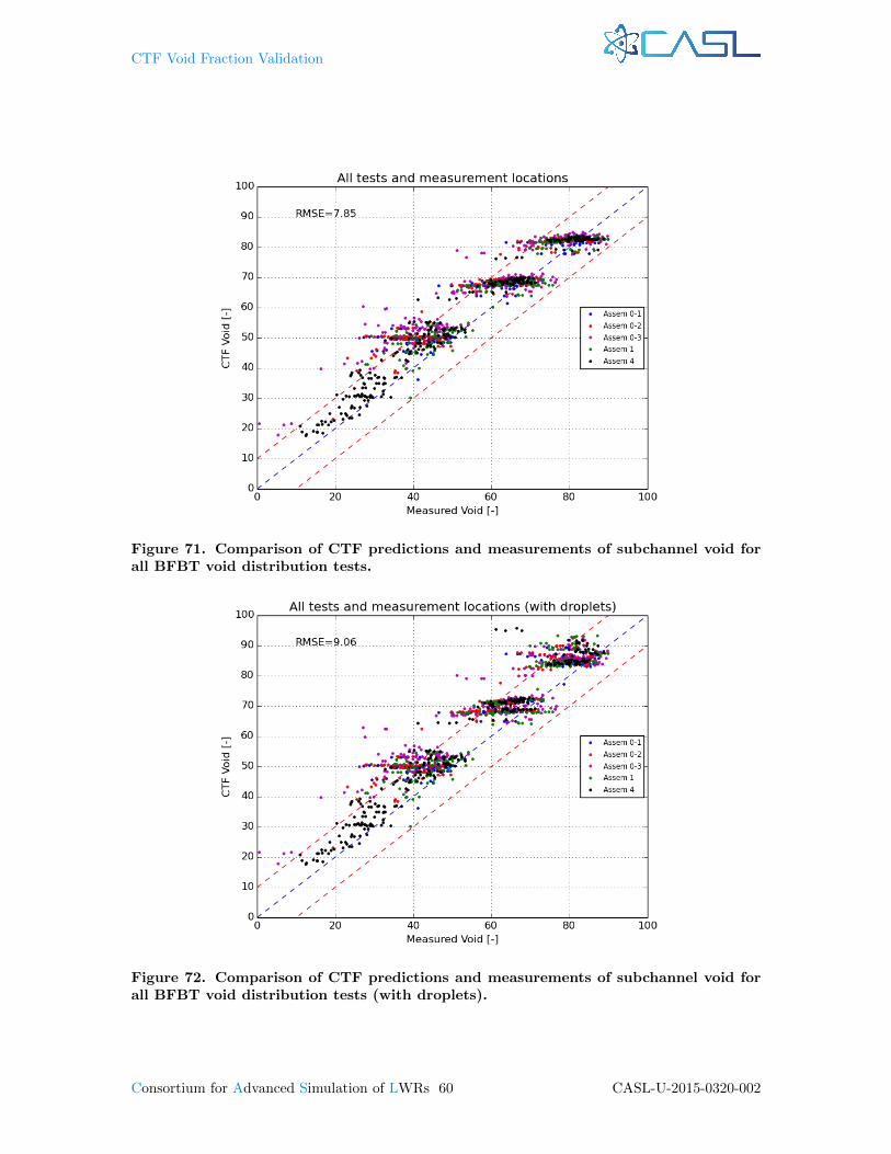
CTF Void Fraction Validation
Figure 71. Comparison of CTF predictions and measurements of subchannel void forall BFBT void distribution tests.
Figure 72. Comparison of CTF predictions and measurements of subchannel void forall BFBT void distribution tests (with droplets).
Consortium for Advanced Simulation of LWRs 60 CASL-U-2015-0320-002
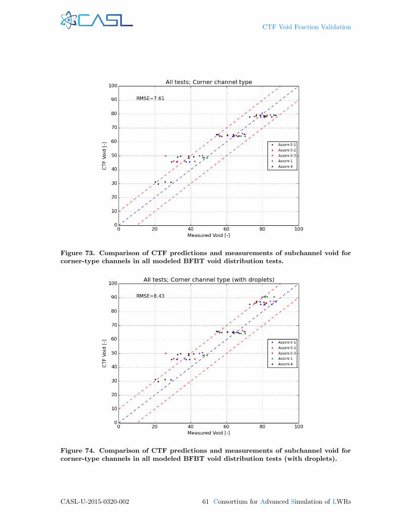
CTF Void Fraction Validation
Figure 73. Comparison of CTF predictions and measurements of subchannel void forcorner-type channels in all modeled BFBT void distribution tests.
Figure 74. Comparison of CTF predictions and measurements of subchannel void forcorner-type channels in all modeled BFBT void distribution tests (with droplets).
CASL-U-2015-0320-002 61 Consortium for Advanced Simulation of LWRs

CTF Void Fraction Validation
Figure 75. Comparison of CTF predictions and measurements of subchannel void forside-type channels in all modeled BFBT void distribution tests.
Figure 76. Comparison of CTF predictions and measurements of subchannel void forside-type channels in all modeled BFBT void distribution tests (with droplets).
Consortium for Advanced Simulation of LWRs 62 CASL-U-2015-0320-002
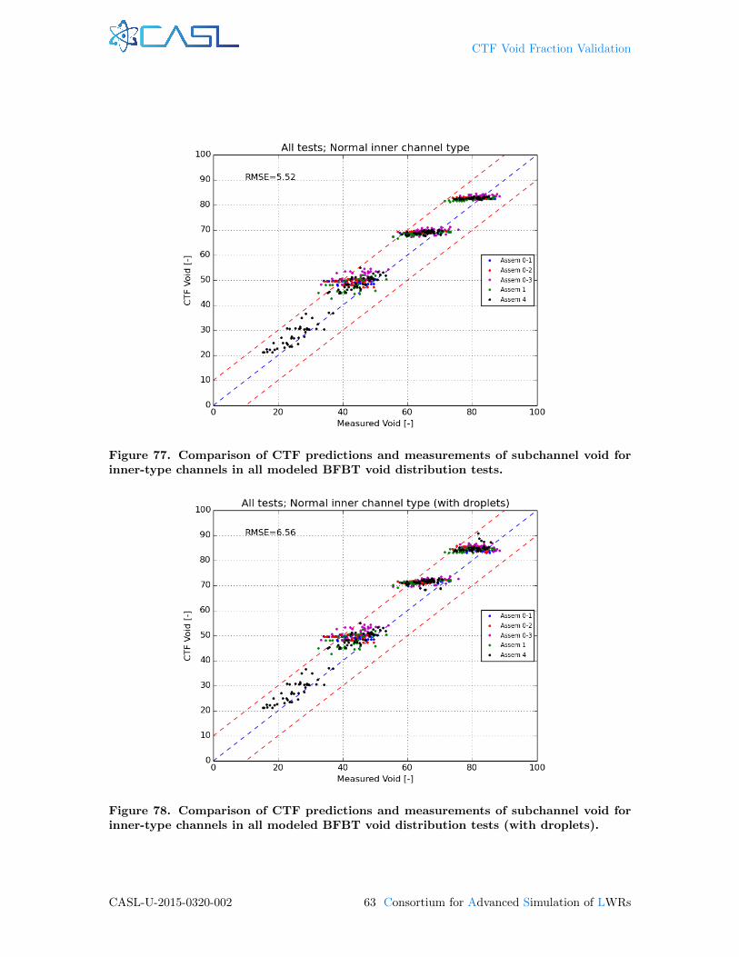
CTF Void Fraction Validation
Figure 77. Comparison of CTF predictions and measurements of subchannel void forinner-type channels in all modeled BFBT void distribution tests.
Figure 78. Comparison of CTF predictions and measurements of subchannel void forinner-type channels in all modeled BFBT void distribution tests (with droplets).
CASL-U-2015-0320-002 63 Consortium for Advanced Simulation of LWRs
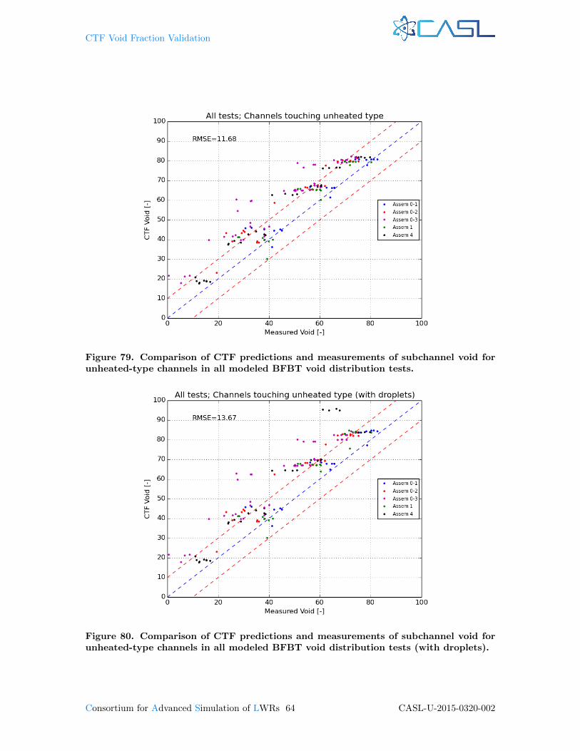
CTF Void Fraction Validation
Figure 79. Comparison of CTF predictions and measurements of subchannel void forunheated-type channels in all modeled BFBT void distribution tests.
Figure 80. Comparison of CTF predictions and measurements of subchannel void forunheated-type channels in all modeled BFBT void distribution tests (with droplets).
Consortium for Advanced Simulation of LWRs 64 CASL-U-2015-0320-002

CTF Void Fraction Validation
Figure 81. Comparison of CTF predictions and measurements of subchannel void for allchannels in all modeled BFBT void distribution tests when void drift model is disabled.
Figure 82. Comparison of CTF predictions and measurements of subchannel void forcorner channels in all modeled BFBT void distribution tests when void drift model isdisabled.
CASL-U-2015-0320-002 65 Consortium for Advanced Simulation of LWRs
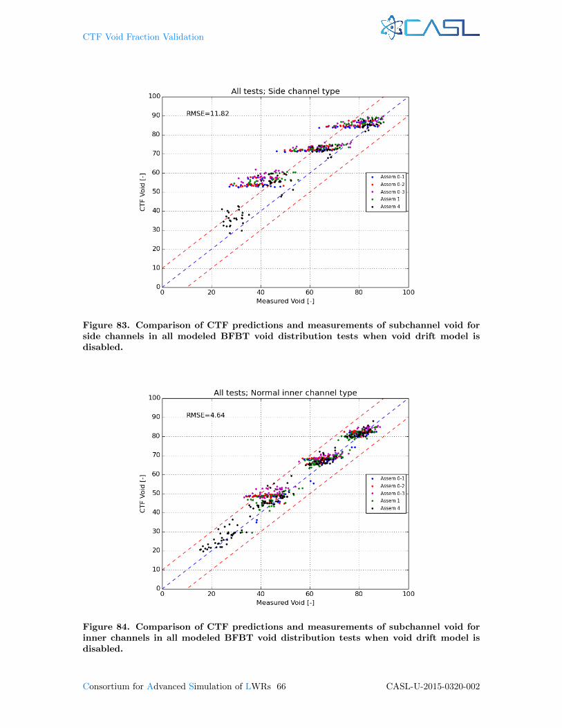
CTF Void Fraction Validation
Figure 83. Comparison of CTF predictions and measurements of subchannel void forside channels in all modeled BFBT void distribution tests when void drift model isdisabled.
Figure 84. Comparison of CTF predictions and measurements of subchannel void forinner channels in all modeled BFBT void distribution tests when void drift model isdisabled.
Consortium for Advanced Simulation of LWRs 66 CASL-U-2015-0320-002

CTF Void Fraction Validation
Figure 85. Comparison of CTF predictions and measurements of subchannel void forunheated channels in all modeled BFBT void distribution tests when void drift modelis disabled.
Table 5. Summary of the CTF predictions of BFBT void distribution cases
Channel No Drops With Drops No Drops
Group With Void Drift With Void Drift No Void Drift
Corner 7.61 8.43 11.47
Side 9.05 10.25 11.82
Inner 5.52 6.56 4.64
Unheated 11.68 13.67 11.56
All 7.85 9.06 8.95
CASL-U-2015-0320-002 67 Consortium for Advanced Simulation of LWRs
CTF Void Fraction Validation
As it has been shown that there is a tendency for CTF to globally over-predict measured voiddata, it is important to use the data to look at trends. In other words, the void drift phenomenacauses void to migrate from smaller area channels to higher area channels. It is important to look forthis behavior in the simulations. The void drift model should be enabled and disabled to observe theimpact of the model on results. To do this, void data is visualized over the diagonals of each assembly.Figure 86 gives an example of the two diagonal lines that are struck through the assemblies. Theexample is given for Assembly Type 0-1, but the process is the same for all five assembly types.Note that the red line goes from the northwest to the southeast, and the blue line goes from thesouthwest to the northeast. The experimental data along these lines will be shown with dots, andthe CTF predictions will be shown with lines. The red dots and lines will be for the northwest tosoutheast diagonal, and the blue dots and lines will be for the southwest to northwest diagonal.
Figure 87 shows results for Test 0011-55, which is from Assembly Type 0-1. Figure 88 showsthe same results, but with the void drift model disabled in the CTF simulation. In both cases, theCTF results are fairly symmetric. The red line has slightly different behavior because the centerof the bundle has two guide tubes that lead to an asymmetric rod placement. In both cases, CTFcaptures the reduction in void in the center of the model because of the presence of the unheatedguide tubes. However, the reduction is not as severe as it is in the experimental results.
Additionally, the experimental results see a jump up in void for the center channel. This behavioris likely due to the design of the spacer grid, which offers no flow resistance to the central subchannel.Despite the central subchannel having a smaller hydraulic diameter than surrounding channels (andthus a higher frictional pressure drop), the lack of a form loss allows the velocity to climb higherthan its neighbors, which causes the higher velocity void to seek the path of least flow resistanceand migrate into the center subchannel.
With void drift disabled, CTF sees a larger drop in void in the center channel than when voiddrift is enabled. Void increasing in the center subchannel is the correct behavior due to the lackof a form loss in that channel. The CTF void drift model acts to move void from lower to highervelocity subchannels, so turning the void drift model on causes void to migrate from the larger areachannels (which have lower velocity) into the center channel (which has higher velocity).
When void drift is enabled, the trend of void decreasing in the corner channels is predicted.When void drift is disabled, the void is highest in the corner channels, which is incorrect. Whilethe trend is predicted correctly, the magnitude of the drop is less in CTF than in the experimentalresults. It is possible that the experimental facility walls are not perfectly adiabatic, which mayexplain the over-prediction of void in CTF. Overall, there is an improvement of about 1 percentagepoint for the RMSE of both lines of CTF predictions when compared to the experimental data.
As has been previously noted, the void drift effect becomes less severe at higher overall bundlevoid content. Test 0011-61 is also run in Assembly Type 0-1; however, it is run at a much higherpower, leading to a bundle average void that is about double that of Test 0011-55. Figure 89 showsthe void distribution on the diagonals with void drift enabled. Figure 90 shows the same data, butwith void drift disabled in the CTF simulations.
It is observed that the CTF results, with void drift enabled, compare very nicely to experimentaldata because the void drift phenomena is not as severe. The RMSE is between 4 and 6 percentagepoints lower than the lower void case, Test 0011-55. Disabling the void drift model actually leadsto an improvement in one of the diagonals when comparing to experimental data due to the largeasymmetry in the corner results.
The low-void test from Assembly 0-2, which has four unheated rods in the bundle center, isshown in Figure 91 with void drift enabled and in Figure 92 with void drift disabled. Similar trendsare observed, but it is noted that void content decreases more in the center than it did in Assembly0-1 due to the disabling of the two center heater rods. As in the case of Assembly Type 0-1, thevoid drift effect is less prominent in the higher void case, which is shown in Figure 93 (with voiddrift) and Figure 94 (without void drift). Note, though, that enabling the void drift model in CTFallows a great deal of void to migrate into the center of the bundle, which is unrealistic comparedwith the experimental results.
Test case 0031-16 is run in Assembly Type 0-3, which has seven unheated rods and two guidetubes in a position that is offset from the center of the bundle. This leads to an asymmetric
Consortium for Advanced Simulation of LWRs 68 CASL-U-2015-0320-002
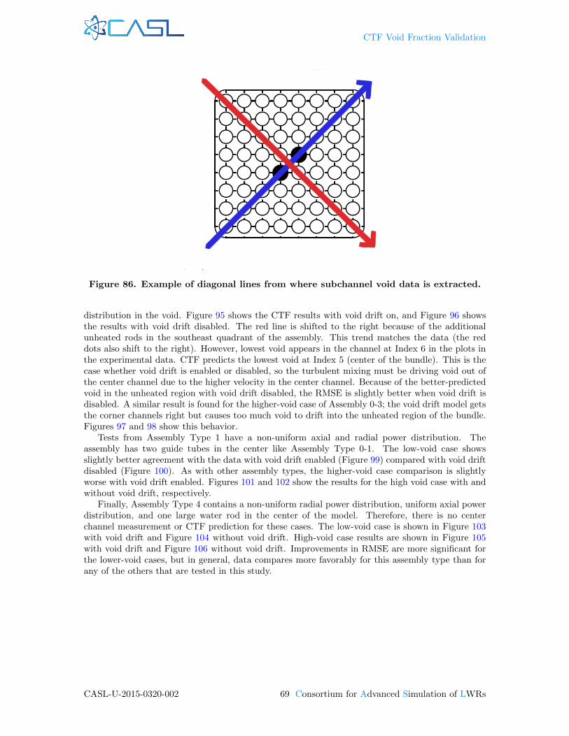
CTF Void Fraction Validation
Figure 86. Example of diagonal lines from where subchannel void data is extracted.
distribution in the void. Figure 95 shows the CTF results with void drift on, and Figure 96 showsthe results with void drift disabled. The red line is shifted to the right because of the additionalunheated rods in the southeast quadrant of the assembly. This trend matches the data (the reddots also shift to the right). However, lowest void appears in the channel at Index 6 in the plots inthe experimental data. CTF predicts the lowest void at Index 5 (center of the bundle). This is thecase whether void drift is enabled or disabled, so the turbulent mixing must be driving void out ofthe center channel due to the higher velocity in the center channel. Because of the better-predictedvoid in the unheated region with void drift disabled, the RMSE is slightly better when void drift isdisabled. A similar result is found for the higher-void case of Assembly 0-3; the void drift model getsthe corner channels right but causes too much void to drift into the unheated region of the bundle.Figures 97 and 98 show this behavior.
Tests from Assembly Type 1 have a non-uniform axial and radial power distribution. Theassembly has two guide tubes in the center like Assembly Type 0-1. The low-void case showsslightly better agreement with the data with void drift enabled (Figure 99) compared with void driftdisabled (Figure 100). As with other assembly types, the higher-void case comparison is slightlyworse with void drift enabled. Figures 101 and 102 show the results for the high void case with andwithout void drift, respectively.
Finally, Assembly Type 4 contains a non-uniform radial power distribution, uniform axial powerdistribution, and one large water rod in the center of the model. Therefore, there is no centerchannel measurement or CTF prediction for these cases. The low-void case is shown in Figure 103with void drift and Figure 104 without void drift. High-void case results are shown in Figure 105with void drift and Figure 106 without void drift. Improvements in RMSE are more significant forthe lower-void cases, but in general, data compares more favorably for this assembly type than forany of the others that are tested in this study.
CASL-U-2015-0320-002 69 Consortium for Advanced Simulation of LWRs
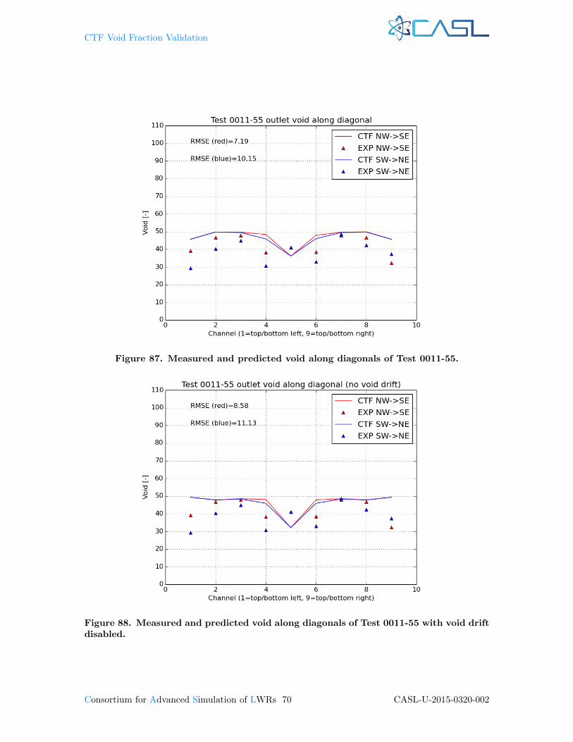
CTF Void Fraction Validation
Figure 87. Measured and predicted void along diagonals of Test 0011-55.
Figure 88. Measured and predicted void along diagonals of Test 0011-55 with void driftdisabled.
Consortium for Advanced Simulation of LWRs 70 CASL-U-2015-0320-002
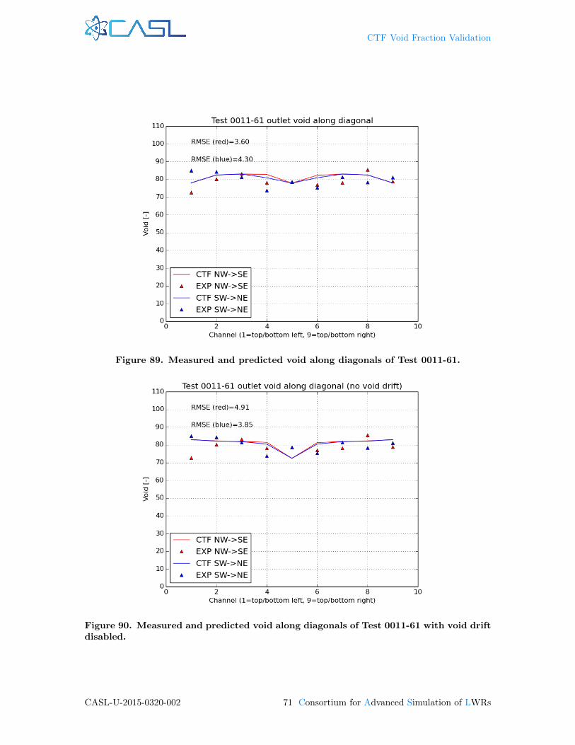
CTF Void Fraction Validation
Figure 89. Measured and predicted void along diagonals of Test 0011-61.
Figure 90. Measured and predicted void along diagonals of Test 0011-61 with void driftdisabled.
CASL-U-2015-0320-002 71 Consortium for Advanced Simulation of LWRs
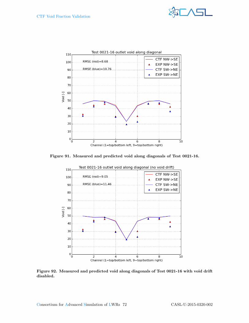
CTF Void Fraction Validation
Figure 91. Measured and predicted void along diagonals of Test 0021-16.
Figure 92. Measured and predicted void along diagonals of Test 0021-16 with void driftdisabled.
Consortium for Advanced Simulation of LWRs 72 CASL-U-2015-0320-002
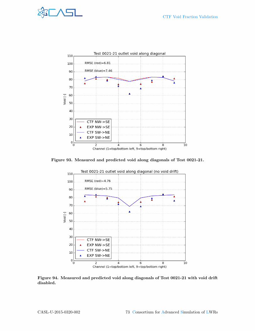
CTF Void Fraction Validation
Figure 93. Measured and predicted void along diagonals of Test 0021-21.
Figure 94. Measured and predicted void along diagonals of Test 0021-21 with void driftdisabled.
CASL-U-2015-0320-002 73 Consortium for Advanced Simulation of LWRs
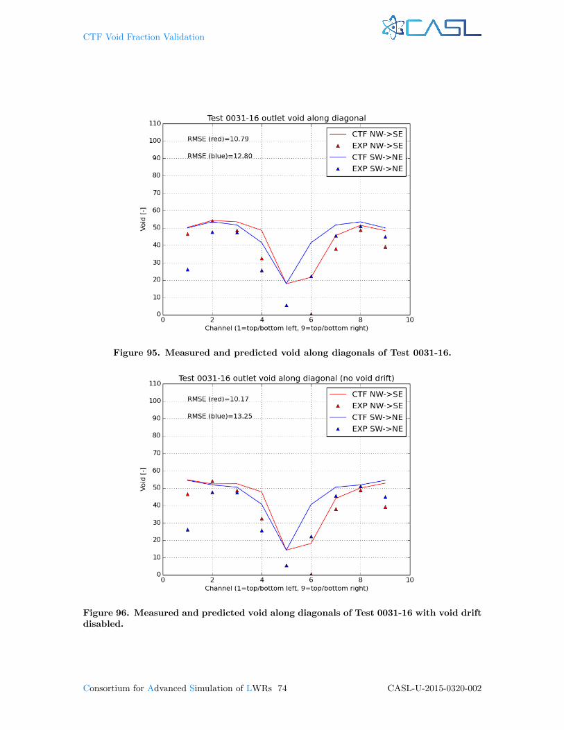
CTF Void Fraction Validation
Figure 95. Measured and predicted void along diagonals of Test 0031-16.
Figure 96. Measured and predicted void along diagonals of Test 0031-16 with void driftdisabled.
Consortium for Advanced Simulation of LWRs 74 CASL-U-2015-0320-002
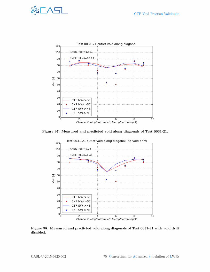
CTF Void Fraction Validation
Figure 97. Measured and predicted void along diagonals of Test 0031-21.
Figure 98. Measured and predicted void along diagonals of Test 0031-21 with void driftdisabled.
CASL-U-2015-0320-002 75 Consortium for Advanced Simulation of LWRs

CTF Void Fraction Validation
Figure 99. Measured and predicted void along diagonals of Test 1071-55.
Figure 100. Measured and predicted void along diagonals of Test 1071-55 with voiddrift disabled.
Consortium for Advanced Simulation of LWRs 76 CASL-U-2015-0320-002
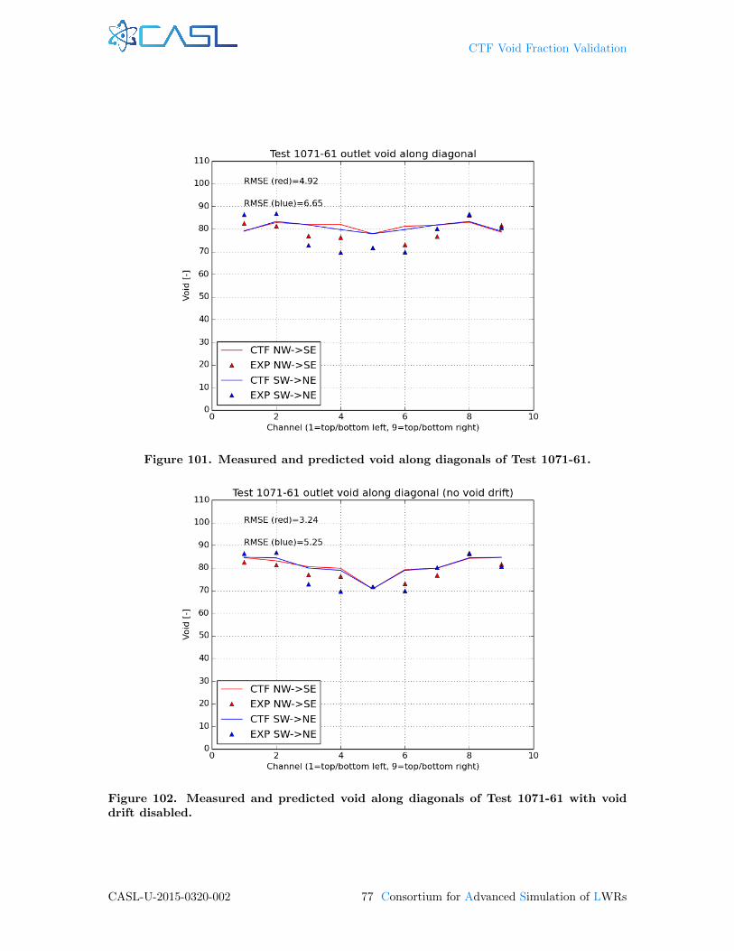
CTF Void Fraction Validation
Figure 101. Measured and predicted void along diagonals of Test 1071-61.
Figure 102. Measured and predicted void along diagonals of Test 1071-61 with voiddrift disabled.
CASL-U-2015-0320-002 77 Consortium for Advanced Simulation of LWRs
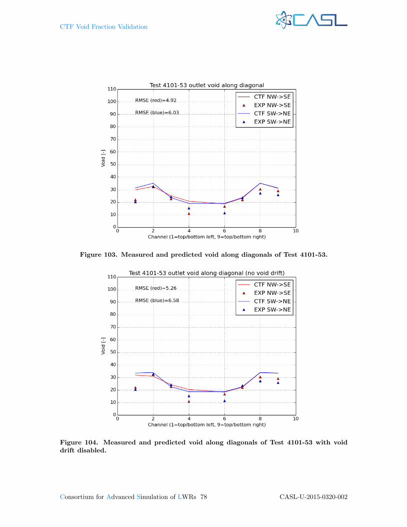
CTF Void Fraction Validation
Figure 103. Measured and predicted void along diagonals of Test 4101-53.
Figure 104. Measured and predicted void along diagonals of Test 4101-53 with voiddrift disabled.
Consortium for Advanced Simulation of LWRs 78 CASL-U-2015-0320-002

CTF Void Fraction Validation
Figure 105. Measured and predicted void along diagonals of Test 4101-61.
Figure 106. Measured and predicted void along diagonals of Test 4101-61 with voiddrift disabled.
CASL-U-2015-0320-002 79 Consortium for Advanced Simulation of LWRs
CTF Void Fraction Validation
4 CONCLUSION
This report documents a study of the CTF turbulent mixing and void drift model. This studyincludes performing verification testing on the single-phase friction and single-phase turbulent mixingmodels, which affect the prediction of rod-bundle flow distribution. It is shown that both of thesemodels are working as intended and compare favorably to analytical solutions.
Validation testing is performed to show how CTF-predicted flow distribution compares to exper-imental data for two facilities: the RPI 2×2 facility and the GE 3×3 facility. The flow reaches theequilibrium distribution for BWR geometry and operating conditions by the end of the 2 m lengthof the GE 3×3 test facility. In the low-pressure, air/water 2×2 facility, the flow distribution doesnot achieve equilibrium conditions until about 5 m of axial length. This result compares poorly withthe experimental measurements, which were taken at the outlet of the 1 m facility.
Moving from single-phase V&V testing to two-phase V&V testing is challenging. First, two-phase flow introduces the competing physical phenomenon of two-phase turbulent mixing and voiddrift, which cannot be separated in experiment. Therefore, individual models in CTF for modelingthese effects cannot be separately tested. Second, it is found difficult to model low-pressure air/water facilities in CTF; the code has a great deal of difficulty in meeting the specified steady-stateconvergence criteria of the code. After many unsuccessful attempts to model the 2×2 air/waterfacility, it is decided that CTF is not currently suitable for modeling the geometry and operatingconditions of the facility. A study has been previously performed with this experiment by using anartificially elevated operating pressure of 100 bar; however, it is also noted that CTF does not seemto converge on a flow distribution that achieves equilibrium by the exit of the facility. Studies shouldbe performed in the future to investigate the severity of the actual solution oscillations (rather thanthe engineering parameters used as convergence metrics) as well as the specific reasons why the CTFsolution fails to converge.
Alternatively, success is found in modeling higher-pressure test facilities that are more repre-sentative of realistic reactor operating conditions. The Validation Manual includes results of thepreviously modeled GE 3×3 facility. This study expands on the previous study with new results andanalysis. This study also adds the BFBT 8×8 void distribution experiments to the test matrix. Theproblem with these facilities is that they drive testing further from separate effects testing by addingadditional complexities, including heating, boiling, implicit heat transfer, non-uniform enthalpy anddensity distribution leading to cross-flow, and spacer grid form losses in the flow. The benefit ofthe air/water tests is they have none of these complexities, allowing for a more direct assessment ofthe void drift and two-phase mixing model in CTF; however, as previously mentioned, CTF is notcurrently suitable for modeling air/water.
The BFBT tests add value to the test matrix because they include several features that are notcovered by the GE tests, including larger test assembly, different spacer grid design, non-uniformaxial and radial power distributions, different measurement technique, and a wider range of operatingconditions. The BFBT study shows that the void drift model is effective in reducing the RMSE byseveral percentage points for lower void test cases (∼10–50% void). At higher void cases (∼80%),the radial void distribution tends to be more uniform, and it is consistently seen that the void driftmodel has a relatively insignificant effect on the accuracy of the results.
In several high void cases, accuracy actually improves with the void drift model disabled. How-ever, it is important to note CTF’s general tendency to overpredict void in the unheated sections ofthe bundle, which has a large impact on this observed trend. Disabling the void drift model keepsvoid from migrating into the center of the bundle and allows CTF predicted void to drop lowerin the unheated center. This region is where most prediction improvements are observed and onlyfor the higher void cases. Similar to the conclusion of the GE validation testing, it is found thatgreatest improvements to predictive capabilities are made for the boundary channels when the voiddrift model is enabled.
It is found that the optimum single-phase mixing coefficient is β=0.007 according to comparisonswith the 2×3 mixing tests. A previous CASL study [10] suggested an optimum value of 0.0044. Sincethe mixing coefficient is dependent on actual gap geometry and flow conditions, this range of valuesprovides bounds on values to use for light water reactor (LWR) analysis. It is found that the
Consortium for Advanced Simulation of LWRs 80 CASL-U-2015-0320-002
CTF Void Fraction Validation
predictive Rogers & Rosehart model tends to over-predict single phase mixing. This degrades theaccuracy of the results for the GE 3×3 single-phase cases compared with using the constant value of0.007. It is found that switching between the two different single-phase mixing models have almostno impact on results accuracy for the two-phase GE 3×3 cases.
The completion of this study results in a more rigorous testing of the void drift model in CTFas well as supporting models that affect the prediction of void drift, including friction and turbulentmixing. The CTF Verification Manual [16] has been updated with the verification tests discussedin this document. The CTF Validation Manual has been updated with the BFBT study discussedin this document. Selected BFBT validation cases have been added to automated CTF regressiontesting to ensure that the results of this study remain valid.
References
[1] R. Lahey and F. Moody. The Thermal-Hydraulics of a Boiling Water Nuclear Reactor. Tech.rep. ANS Monograph, 1977.
[2] R.K. Salko and M.N. Avramova. CTF Theory Manual. The Pennsylvania State University.2012.
[3] R. Sterner and R. Lahey. Air/Water Subchannel Measurements of the Equilibrium Quality andMass Flux Distribution in a Rod Bundle. Tech. rep. Rensselaer Polytechnic Institute, 1983.
[4] R. Salko et al. CTF Validation Manual. Tech. rep. CASL-U-2014-0169-000. Consortium forAdvanced Simulation of Light Water Reactors, 2015.
[5] N. Todreas and M. Kazimi. Nuclear Systems II: Elements of Thermal Hydraulic Design. Hemi-sphere Publishing Corporation, 1990.
[6] M. Sadatomi et al. “Single- and Two-Phase Turbulent Mixing Rate between Adjacent Sub-chanels in a Vertical 2×3 Rod Array Channel”. In International Journal of Multiphase Flow30 (2004), pp. 481–498.
[7] M. Sadatomi et al. “Flow Characteristics in Hydraulically Equilibrium Two-Phase Flows in aVertical 2×3 Rod Bundle Channel”. In International Journal of Multiphase Flow 30 (2004),pp. 1093–1119.
[8] M. Sadatomi, Y. Sato, and S. Saruwatari. “Two-Phase Flow in Vertical Noncircular Channels”.In International Journal of Multiphase Flow 8 (1982), pp. 641–645.
[9] Z. Karoutas et al. Subcooled Boiling Data from Rod Bundles. Tech. rep. 1003383. EPRI, 2002.
[10] Y. Sung et al. Application of Multi-Scale Thermal-Hydraulic Models to DNB Analysis. Tech.rep. CASL-U-2014-0119-000. Consortium for Advanced Simulation of Light Water Reactors,2014.
[11] R. Lahey Jr., B. Shirlakar, and D. Radcliffe. Two-Phase Flow and Heat Transfer In MultirodGeometries: Subchannel and Pressure Drop Measurements in a Nine-Rod Bundle for Diabaticand Adiabatic Conditions. Tech. rep. General Electric, 1970.
[12] B. Neykov et al. NUPEC BWR Full-size Fine-mesh Bundle Test (BFBT) Benchmark. Tech.rep. Nuclear Energy Agency, 2006.
[13] B. Shiralkar and D. Radcliffe. An Experimental and Analytical Study of the Synthesis of GridSpacer Loss Coefficients. Tech. rep. NEDE-13181. General Electric, 1971.
[14] M. Avramova, K. Ivanov, and L. Hochreiter. “Analysis of Steady State and Transient VoidDistribution Predictions for Phase I of the OECD/NEA BFBT Benchmark using CTF/NEM”.In The 12th International Topical Meeting on Nuclear Reactor Thermal Hydraulics (NURETH-12). 2007.
[15] B. Neykov, M. Avramova, and K. Ivanov. “Phase I—Void Distribution Final Results”. In 6th
OECD/NRC BFBT Workshop. 2009.
CASL-U-2015-0320-002 81 Consortium for Advanced Simulation of LWRs

CTF Void Fraction Validation
[16] R. Salko, C. Jernigan, and J. Kelly. CTF Verification Manual. Tech. rep. CASL-U-2015-XXXX-000. Consortium for Advanced Simulation of Light Water Reactors, 2015.
Consortium for Advanced Simulation of LWRs 82 CASL-U-2015-0320-002