Module 11

Quantifying Late Detection in MC&A for Bulk Processes

Module 11-2

Learning Objective

• Familiarization with the probability with which the

Safeguards systems can detect a diversion of material

due to insider activity

• Become familiar with the concept of Statistical Process

Control

Material Balance Evaluation from the Insider Perspective

• Goal is to determine the probability with which the

Safeguards systems can detect a diversion of material

due to insider activity.

• Generally relates to bulk processing.

“Bulk Material – Material in any physical form that is not identifiable

as a discrete item and therefore must be accounted for by weight,

volume, sampling, chemical analysis, or non-destructive

analysis”

• Statistical Process Control is the key underlying concept

or discipline

Module 11-3

Overview

• Inventory differences (IDs)

• Process Control – statistical methods and control charts

• Discuss with respect to the hypothetical process

• Discuss the calculation of Limits-of-Error for inventory

differences (LEIDs)

Module 11-4

Inventory Difference Calculation

The ID is calculated as follows:

ID = BI + TI – TO – EI

Where,

ID = Inventory Difference

BI = Beginning Inventory (prior period physical inventory value)

TI = Transfers In (additions) during the current inventory period

TO = Transfers Out (removals) during the current inventory period

EI = Ending Inventory (current period physical inventory value )

Module 11-5

Inventory Differences

• For an item facility, the ID should always be zero unless an item is

missing.

• For a bulk facility,

The ID is typically different from zero due to measurement

uncertainties, unmeasured holdup, and losses.

The holdup can be treated by estimating the amount in various

pieces of equipment, perhaps based on experiments.

Under ideal conditions, the bulk facility IDs should vary about

zero. (note: systematic differences may cause this not to be the case).

Module 11-6

Simplified ID Example for an Item Facility

Reactor Core:

BI = 60 core fuel assemblies

TI = 20 fresh fuel assemblies

TO = 20 spent fuel assemblies

EI = 60 core fuel assemblies

ID = 60 + 20 - 20 - 60 = 0

Module 11-7

Simplified ID example for a bulk facility

Fabrication Plant Process Area:

BI = 203.5 kg U in beginning process inventory

TI = 600.1 kg U in oxide powder feed

TO = 604.8 kg U in pellet product

EI = 195.6 kg U in ending process inventory

ID = 203.5 + 600.1 - 604.8 - 195.6 = 3.2 kg U

Module 11-8

Making sense of the ID with respect to the Insider

• What techniques can be used to monitor it?

• How does it relate to the insider analysis in the

vulnerability assessment?

• When is it or how much of an ID is significant?

MOST IMPORTANTLY….

• What are we trying to detect?

Module 11-9

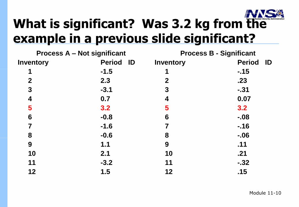
What is significant? Was 3.2 kg from the example in a previous slide significant?

Process A – Not significant

Inventory Period ID

1 -1.5

2 2.3

3 -3.1

4 0.7

5 3.2

6 -0.8

7 -1.6

8 -0.6

9 1.1

10 2.1

11 -3.2

12 1.5

Process B - Significant

Inventory Period ID

1 -.15

2 .23

3 -.31

4 0.07

5 3.2

6 -.08

7 -.16

8 -.06

9 .11

10 .21

11 -.32

12 .15

Module 11-10

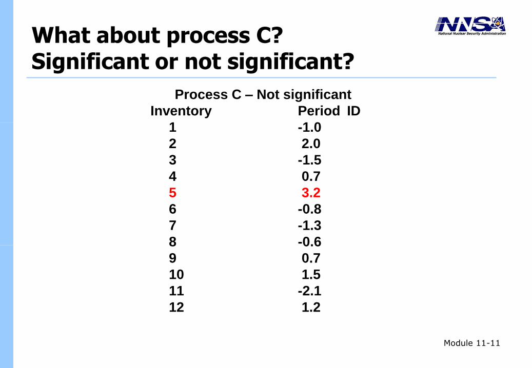
What about process C? Significant or not significant?

Process C – Not significant

Inventory Period ID

1 -1.0

2 2.0

3 -1.5

4 0.7

5 3.2

6 -0.8

7 -1.3

8 -0.6

9 0.7

10 1.5

11 -2.1

12 1.2

Module 11-11

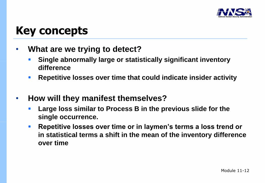
Key concepts

• What are we trying to detect?

Single abnormally large or statistically significant inventory

difference

Repetitive losses over time that could indicate insider activity

• How will they manifest themselves?

Large loss similar to Process B in the previous slide for the

single occurrence.

Repetitive losses over time or in laymen’s terms a loss trend or

in statistical terms a shift in the mean of the inventory difference

over time

Module 11-12

Process or Product Monitoring and Control

• Shewart Control Charts

• Cumulative Sum (CUSUM) Control Charts

• Exponentially Weighted Moving Average (EWMA) Control Charts

• MOST IMPORTANT PART Average Run Length (ARL)

• When the process is operating at the target mean and a shift of magnitude δ occurs the number of inventories it takes to detect the shift.

Generally CUSUM or EWMA are better at 2 sigma or less while Shewart is better at greater than 2 sigma.

Module 11-13

Average Run Length to Detect a 1 Sigma Shift in the Process Average for the Various Techniques

• Shewart Charts will detect a 1 sigma (standard deviation)

shift in the mean in around 42-44 inventories

• Both CUSUM and EWMA will detect a 1 sigma shift in

about 10 inventories

• As the shift in the mean gets smaller all techniques

converge on 370 inventories

• As the shift in the mean gets larger (e.g., around 2.5

sigma or greater) Shewart is more effective

Note: Under current DOE regulations an ID > 2 sigma (warning limit) will be

investigated regardless.

Module 11-14

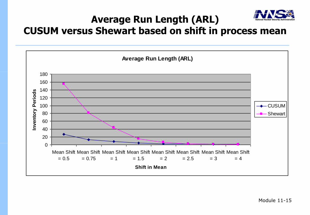
Average Run Length (ARL) CUSUM versus Shewart based on shift in process mean

Average Run Length (ARL)

0

20

40

60

80

100

120

140

160

180

Mean Shift

= 0.5

Mean Shift

= 0.75

Mean Shift

= 1

Mean Shift

= 1.5

Mean Shift

= 2

Mean Shift

= 2.5

Mean Shift

= 3

Mean Shift

= 4

Shift in Mean

Inven

tory

Peri

od

s

CUSUM

Shewart

Module 11-15

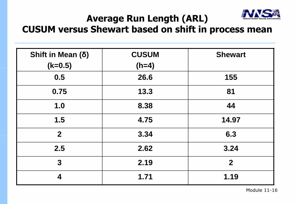
Average Run Length (ARL) CUSUM versus Shewart based on shift in process mean

Shift in Mean (δ)

(k=0.5)

CUSUM

(h=4)

Shewart

0.5 26.6 155

0.75 13.3 81

1.0 8.38 44

1.5 4.75 14.97

2 3.34 6.3

2.5 2.62 3.24

3 2.19 2

4 1.71 1.19

Module 11-16

Shewart Charts

• First proposed during the 1920’s by Dr. Walter A. Shewart

UCL = Process Mean + k (standard deviation)

Center Line = Process Mean or target

LCL = Process Mean – k (standard deviation)

Module 11-17

Inventory Difference X

7.8UCL

0.0CL

-7.8LCL

-10.4

-8.4

-6.4

-4.4

-2.4

-0.4

1.6

3.6

5.6

7.6

9.6

Date/Time/Period

Inven

tory

Dif

fere

nce

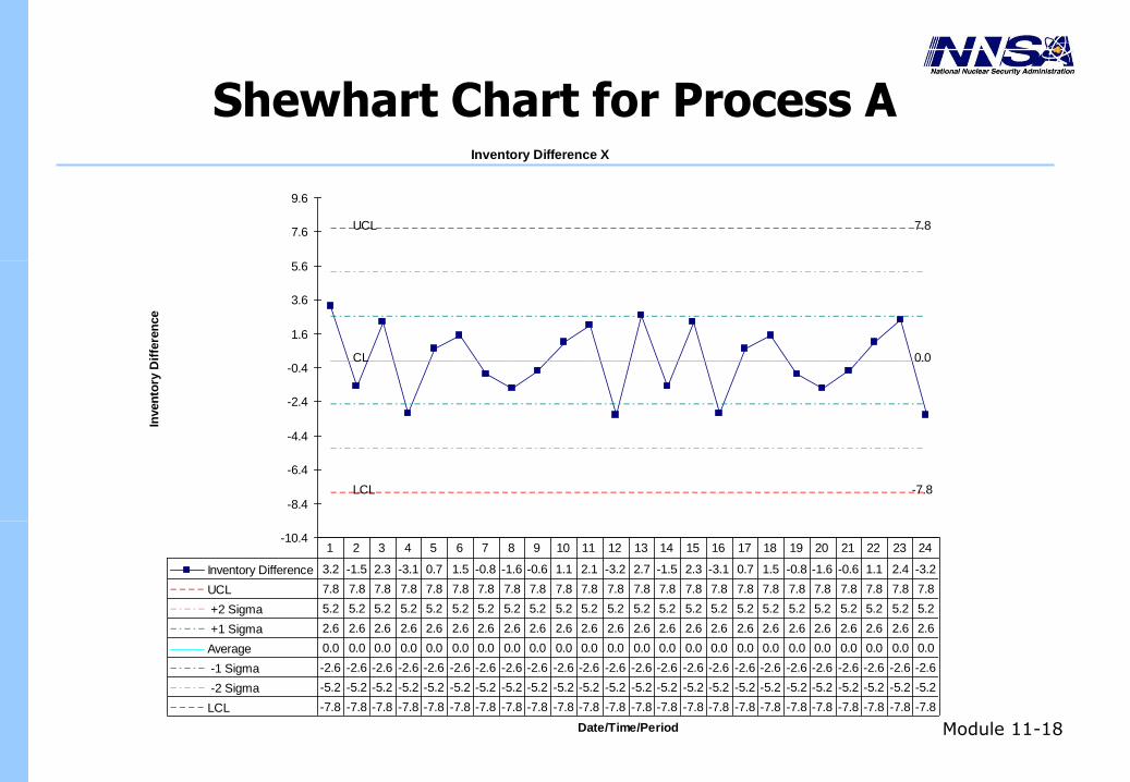
Inventory Difference 3.2 -1.5 2.3 -3.1 0.7 1.5 -0.8 -1.6 -0.6 1.1 2.1 -3.2 2.7 -1.5 2.3 -3.1 0.7 1.5 -0.8 -1.6 -0.6 1.1 2.4 -3.2

UCL 7.8 7.8 7.8 7.8 7.8 7.8 7.8 7.8 7.8 7.8 7.8 7.8 7.8 7.8 7.8 7.8 7.8 7.8 7.8 7.8 7.8 7.8 7.8 7.8

+2 Sigma 5.2 5.2 5.2 5.2 5.2 5.2 5.2 5.2 5.2 5.2 5.2 5.2 5.2 5.2 5.2 5.2 5.2 5.2 5.2 5.2 5.2 5.2 5.2 5.2

+1 Sigma 2.6 2.6 2.6 2.6 2.6 2.6 2.6 2.6 2.6 2.6 2.6 2.6 2.6 2.6 2.6 2.6 2.6 2.6 2.6 2.6 2.6 2.6 2.6 2.6

Average 0.0 0.0 0.0 0.0 0.0 0.0 0.0 0.0 0.0 0.0 0.0 0.0 0.0 0.0 0.0 0.0 0.0 0.0 0.0 0.0 0.0 0.0 0.0 0.0

-1 Sigma -2.6 -2.6 -2.6 -2.6 -2.6 -2.6 -2.6 -2.6 -2.6 -2.6 -2.6 -2.6 -2.6 -2.6 -2.6 -2.6 -2.6 -2.6 -2.6 -2.6 -2.6 -2.6 -2.6 -2.6

-2 Sigma -5.2 -5.2 -5.2 -5.2 -5.2 -5.2 -5.2 -5.2 -5.2 -5.2 -5.2 -5.2 -5.2 -5.2 -5.2 -5.2 -5.2 -5.2 -5.2 -5.2 -5.2 -5.2 -5.2 -5.2

LCL -7.8 -7.8 -7.8 -7.8 -7.8 -7.8 -7.8 -7.8 -7.8 -7.8 -7.8 -7.8 -7.8 -7.8 -7.8 -7.8 -7.8 -7.8 -7.8 -7.8 -7.8 -7.8 -7.8 -7.8

1 2 3 4 5 6 7 8 9 10 11 12 13 14 15 16 17 18 19 20 21 22 23 24

Shewhart Chart for Process A

Module 11-18

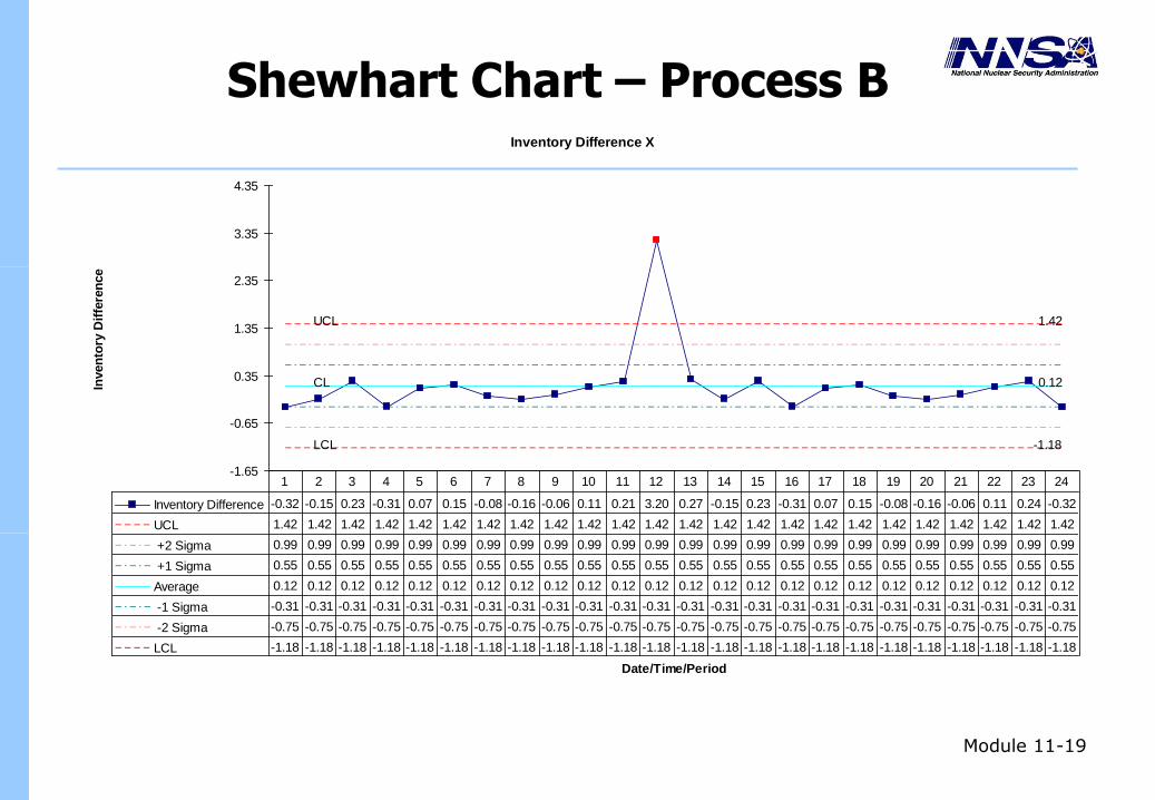
Shewhart Chart – Process B Inventory Difference X

1.42UCL

0.12CL

-1.18LCL

-1.65

-0.65

0.35

1.35

2.35

3.35

4.35

Date/Time/Period

Inven

tory

Dif

fere

nce

Inventory Difference -0.32 -0.15 0.23 -0.31 0.07 0.15 -0.08 -0.16 -0.06 0.11 0.21 3.20 0.27 -0.15 0.23 -0.31 0.07 0.15 -0.08 -0.16 -0.06 0.11 0.24 -0.32

UCL 1.42 1.42 1.42 1.42 1.42 1.42 1.42 1.42 1.42 1.42 1.42 1.42 1.42 1.42 1.42 1.42 1.42 1.42 1.42 1.42 1.42 1.42 1.42 1.42

+2 Sigma 0.99 0.99 0.99 0.99 0.99 0.99 0.99 0.99 0.99 0.99 0.99 0.99 0.99 0.99 0.99 0.99 0.99 0.99 0.99 0.99 0.99 0.99 0.99 0.99

+1 Sigma 0.55 0.55 0.55 0.55 0.55 0.55 0.55 0.55 0.55 0.55 0.55 0.55 0.55 0.55 0.55 0.55 0.55 0.55 0.55 0.55 0.55 0.55 0.55 0.55

Average 0.12 0.12 0.12 0.12 0.12 0.12 0.12 0.12 0.12 0.12 0.12 0.12 0.12 0.12 0.12 0.12 0.12 0.12 0.12 0.12 0.12 0.12 0.12 0.12

-1 Sigma -0.31 -0.31 -0.31 -0.31 -0.31 -0.31 -0.31 -0.31 -0.31 -0.31 -0.31 -0.31 -0.31 -0.31 -0.31 -0.31 -0.31 -0.31 -0.31 -0.31 -0.31 -0.31 -0.31 -0.31

-2 Sigma -0.75 -0.75 -0.75 -0.75 -0.75 -0.75 -0.75 -0.75 -0.75 -0.75 -0.75 -0.75 -0.75 -0.75 -0.75 -0.75 -0.75 -0.75 -0.75 -0.75 -0.75 -0.75 -0.75 -0.75

LCL -1.18 -1.18 -1.18 -1.18 -1.18 -1.18 -1.18 -1.18 -1.18 -1.18 -1.18 -1.18 -1.18 -1.18 -1.18 -1.18 -1.18 -1.18 -1.18 -1.18 -1.18 -1.18 -1.18 -1.18

1 2 3 4 5 6 7 8 9 10 11 12 13 14 15 16 17 18 19 20 21 22 23 24

Module 11-19

Shewart Charts Advantages/Disadvantages

Advantages

• Very effective at detecting large process shifts

Disadvantages

• Not so good for trends because it only uses information

contained in the last data point

Can address some of the disadvantages with respect to

trends by applying the Western Electric Company Rules

(WECO) for signaling out of control situations.

Module 11-20

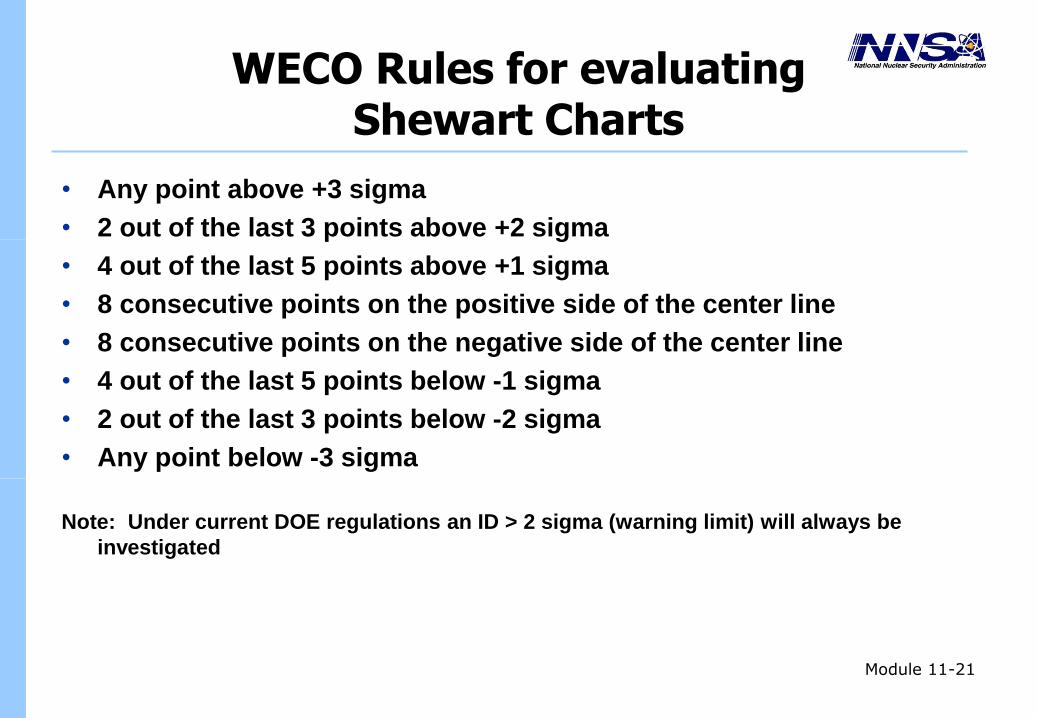
WECO Rules for evaluating Shewart Charts

• Any point above +3 sigma

• 2 out of the last 3 points above +2 sigma

• 4 out of the last 5 points above +1 sigma

• 8 consecutive points on the positive side of the center line

• 8 consecutive points on the negative side of the center line

• 4 out of the last 5 points below -1 sigma

• 2 out of the last 3 points below -2 sigma

• Any point below -3 sigma

Note: Under current DOE regulations an ID > 2 sigma (warning limit) will always be

investigated

Module 11-21

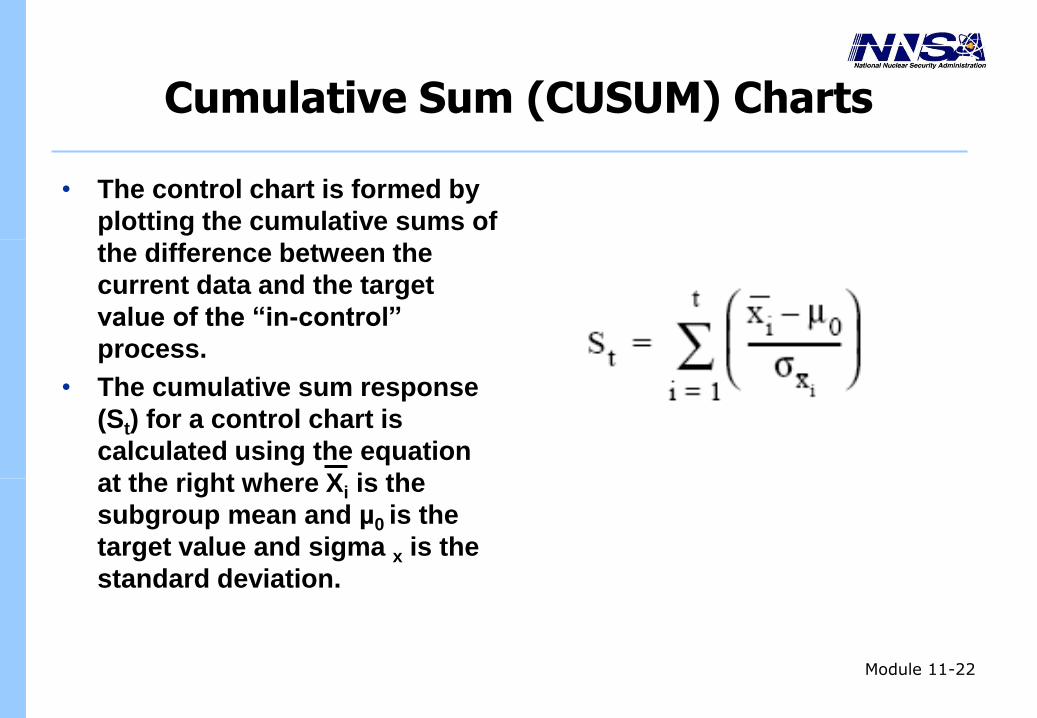
Cumulative Sum (CUSUM) Charts

• The control chart is formed by

plotting the cumulative sums of

the difference between the

current data and the target

value of the “in-control”

process.

• The cumulative sum response

(St) for a control chart is

calculated using the equation

at the right where Xi is the

subgroup mean and µ0 is the

target value and sigma x is the

standard deviation.

Module 11-22

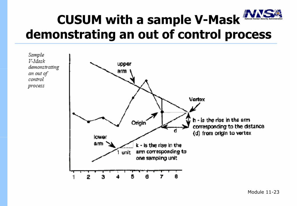
CUSUM with a sample V-Mask demonstrating an out of control process

Module 11-23

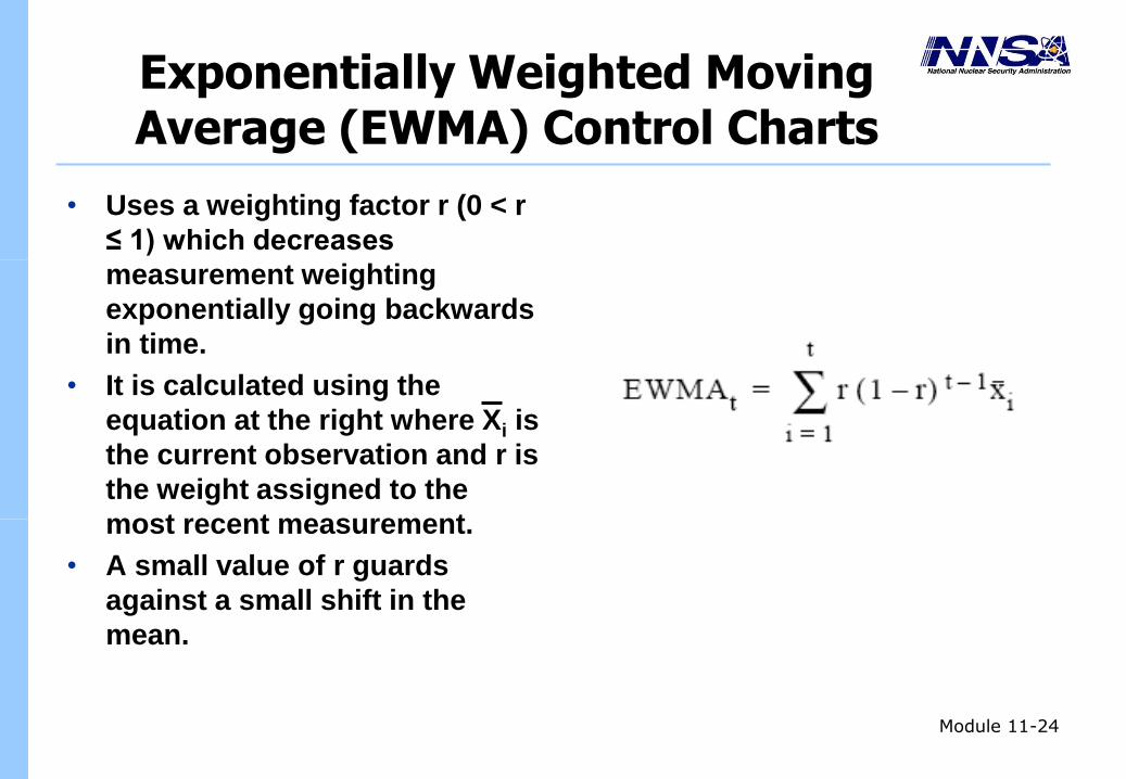
Exponentially Weighted Moving Average (EWMA) Control Charts

• Uses a weighting factor r (0 < r

≤ 1) which decreases

measurement weighting

exponentially going backwards

in time.

• It is calculated using the

equation at the right where Xi is

the current observation and r is

the weight assigned to the

most recent measurement.

• A small value of r guards

against a small shift in the

mean.

Module 11-24

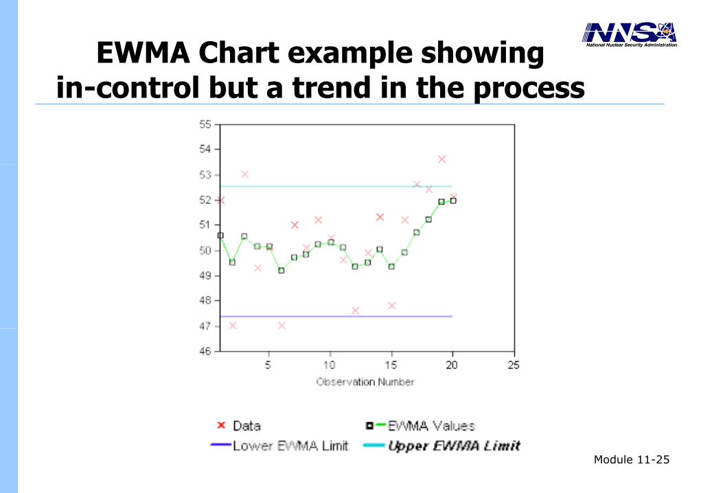
EWMA Chart example showing in-control but a trend in the process

Module 11-25

CUSUM and EWMA Charts Advantages/Disadvantages

Advantages

• Very effective at detecting small process shifts

Disadvantages

• Not as effective as Shewart charts (e.g., 2 sigma or

greater)

• CUSUM is not as intuitive and generally requires

specialized software

Module 11-26

EXERCISE

• Simulate various theft scenarios and how the charting

techniques react.

Module 11-27

Summary

• Process shifts in the inventory of 2 sigma or greater are relatively easy to detect (e.g., significant statistically) within 1 inventory period Shewart charting approach most effective

• Process shifts in the inventory of 1-2 sigma will be detected within 10 inventory periods CUSUM or EWMA tend to be more effective although Shewart with

WECO rules applied can be effective

• Process shifts in the inventory of 0-1 sigma, while not be statistically significant may be seen using the techniques discussed previously (note: timeline for Probability of Detection (Pd) variable)

Module 11-28