Journal of Electroanalytical Chemistry 622 (2008) 225–232

Contents lists available at ScienceDirect

Journal of Electroanalytical Chemistry

journal homepage: www.elsevier .com/locate / je lechem

Current pulse method for in situ measurement of electrochemical capacitance

Graeme A. Snook *, Andrew J. Urban, Marshall R. Lanyon, Katherine McGregorCSIRO Minerals, Box 312, Clayton South, Vic. 3169, Australia

a r t i c l e i n f o

Article history:Received 9 April 2008Received in revised form 4 June 2008Accepted 9 June 2008Available online 15 June 2008

Keywords:Current pulseCapacitance measurementMolten salt electrochemistryResistometerSupercapacitorsAC impedance

0022-0728/$ - see front matter � 2008 Elsevier B.V. Adoi:10.1016/j.jelechem.2008.06.010

* Corresponding author. Tel.: +61 395458863; fax:E-mail address: Graeme.Snook@csiro.au (G.A. Snoo

a b s t r a c t

More than 20 years ago, CSIRO developed an instrument that measures uncompensated resistance simul-taneously with constant voltage, constant current or cyclic voltammetric measurements. The instrument,known as a ‘resistometer’ applies a square current pulse (typically I = 1 A, Dt = 70 ls) and measures theresultant voltage pulse to calculate uncompensated resistance (R = V/I). In the present work, modificationof this instrument has allowed in situ measurement of capacitance as well as resistance by measurementof the voltage change from before application of the pulse to during the rest period of the pulse (C = I � Dt/DV). Testing with a dummy cell (a Randles Equivalent circuit) with capacitances from 10 lF to 1 mF con-firms this relationship and measures the capacitance to within 10% error. Aqueous cyclic voltammetricmeasurements on metal disk working electrodes at the millimetre scale validate the in situ electrochem-ical measurement. Larger electrodes, however, with capacitances in the mF range show a lower fre-quency-dependent value of capacitance when compared to measurements derived from AC impedancetechniques. Measurements in molten salts show increasing capacitance with increasing depth of a copperrod immersed in a CaCl2 bath (950 �C) as expected.

� 2008 Elsevier B.V. All rights reserved.

1. Introduction

One of the difficulties facing researchers in the area of moltensalt electrometallurgy is that the processes that occur at the elec-trode surfaces cannot be easily observed during the course of theelectrolysis. Consequently, it is often difficult to interpret changesin cell current and voltage and relate these unequivocally to elec-trode processes. These must be inferred upon completion of theelectrolysis and removal of the electrodes from the cell. It is pro-posed that a wealth of information could be obtained from in situcapacitance measurements.

A common method for measuring uncompensated (ohmic)resistance and capacitance during electrochemical processes isAC impedance spectroscopy. Obtaining continuous measurementsfrom this technique during electrowinning in molten salts, how-ever, has proven difficult due to vigorous gas evolution at the an-ode. This causes non-steady-state conditions to arise, as well asan unacceptable level of noise. In general, measurements of the cellresistance using this technique are obtained before and after theelectrowinning experiment. Recently in this laboratory the analysisof titanium electrowinning experiments in chloride baths has beengreatly enhanced by the use of an instrument known as the ‘resis-tometer’ [1,2]. This instrument, first developed at CSIRO more than20 years ago, has the ability to measure uncompensated resistancesimultaneously with constant current or constant voltage operat-

ll rights reserved.

+61 395628919.k).

ing conditions. The CSIRO resistometer applies a square, bipolar(typically 1 A) current pulse over a small time-scale (210 ls) tomeasure the resistance. The device works on the principle that acurrent pulse will cause a corresponding voltage pulse accordingto the simple equation:

Vpulse ¼ IpulseRuncompensated ð1Þ

where Vpulse is the jump in voltage after application of the cur-rent pulse (Ipulse), from which the uncompensated resistance(Runcompensated) can be calculated. The uncompensated resistance isdefined as the sum of the

� resistance of the electrolyte between the working electrode andthe surface of the reference electrode (constant);

� resistance of the working electrode body and wire connecting tothe potentiostat (constant);

� resistance of the interphasial region in which the electrode reac-tions are taking place, which can be attributed to changes in thestructure of the electrode (time-varying).

The ability to determine the IR-free voltage continuouslyduring electrowinning experiments in molten salts has beenparticularly useful, and has allowed us to more accurately compen-sate for the IR-drop in our cells for currents of up to 10 A. The mea-surement is applied as a rapid interrupted signal and does notdisturb the electrolysis measurement. This paper describes theadapting of this instrument to measure capacitance as well asresistance.

Fig. 1. Experimental setup for a typical high temperature molten salt TiO2

reduction experiment.

226 G.A. Snook et al. / Journal of Electroanalytical Chemistry 622 (2008) 225–232

Kisza [3,4] has studied the AC impedance of molten salts andthe implications of the double-layer and double layer capacitance.When the solute is also the ionic species (i.e. an ionic liquid) theformation of a double layer and its exact nature in a molten saltis complicated. In molten salt electrochemistry, we believe thatthe measurement of capacitance could provide useful additionalexperimental information. If we assume that the counter-electrodeis sufficiently large, then the measurement of capacitance shouldgive the capacitance of the working electrode of interest. Thecapacitance (C) is proportional to the area of this electrode exposedto the molten salt [5]:

C ¼ eAL

ð2Þ

or

C ¼ Cspecific � A ð3Þ

where e is the permittivity, A is the area, L is the equivalent spac-ing of the capacitor plates (i.e. the double layer separation), andCspecific is the specific capacitance. This means that the relativeelectrode area exposed to the molten salt bath can be measured.This would allow creep of the electrolyte along the electrode sur-face and the ingress of electrolyte into pores in such an experi-ment to be observed. A typical TiO2 electrolysis experimentalsetup is shown in Fig. 1. The measurement of creep is particularlyimportant when excessive electrolyte creep can cause corrosion ofthe electrode holder and consequent failure of the electrode. Ifsurface oxides are formed then a change in Cspecific will be seen.Moreover, if the electrode is consumed or falls apart, this will beobserved as a rapid drop or change in capacitance. We also believethat capacitance may be a more sensitive measure of melting andfreezing of the molten salt electrolyte than a resistance measure-ment. For example, as the melt freezes the resistance will slowlyincrease but will not show a clear transition for freezing as thereare still small conductive pathways of molten electrolyte in thecooling bath. The capacitance, however, should rapidly change asthe interface between the electrolyte and the electrode freezes.All these observations provide in situ information about the mol-ten salt electrolysis measurement.

This technique could also be applied to room temperature mea-surements such as conducting polymer tests (on thin layers at-tached to electrodes) [6,7]. This would be analogous to the typeof measurements done on thin layers for Quartz Crystal Microbal-ance measurements [8,9].

2. Experimental

A dummy cell was constructed from a 1 X resistor (5% toler-ance) and a wound 100 X resistor, as well as a series of capacitorsincluding an Elna 1 mF (10% tolerance) capacitor. The additionalresistance for testing of the effect of Faradaic and solution resis-tance was added into the circuit using a Sample Electronics resistordecade box.

Water obtained from a MilliQ Reagent System (18 MX cm resis-tivity) was used for the preparation of all aqueous electrolyte solu-tions. Aqueous measurements were performed using a Solartron SI1286 Interface (cyclic voltammetry) and a Solartron SI 1255 HF fre-quency response analyser (AC impedance). A three electrode setupwas used, with a platinum mesh counter-electrode and Ag/AgCl(3 M KCl(aq)) reference electrode. The working electrodes were aglassy carbon disk electrode (2 mm diameter), a platinum diskelectrode (1.6 mm diameter), a platinum flag electrode (38 mm �7.3 mm) and a sheathed carbon rod electrode (16.7 mm long �6.6 mm diameter).

Capacitance measurements of a copper rod (3.3 mm diameter)dipped to different depths into the molten salt (CaCl2) were per-

formed using a EG&G PAR Model 362 scanning potentiostat. Exper-imental details for the furnace, cell and molten salt preparation aregiven elsewhere [10]. In the bottom of the crucible, �40 g of titaniapaste was dried in a dish and connected as a cathode using a kan-thal strip in the titania and an alumina sheathed kanthal wireextending out of the furnace. Sheathing was required to preventcorrosion or molten salt attack of the kanthal wire. The upper partof a copper rod was sheathed with an alumina tube and the ex-posed part was lowered into the bath while electrically connectedto the potentiostat and resistometer. The depth required to dip theelectrode was calculated using a copper dip test. This involved dip-ping a copper rod into the bath and marking the top of the furnaceport on the rod and removing the rod. This is performed at suffi-ciently rapid rate, such that the CaCl2 freezes onto the rod allowingmeasurement of the depth of the molten salt bath and the distancefrom the top of the furnace port to the top of the bath. Absolutedetermination of when the copper rod was touching the top ofthe molten salt bath was achieved by measuring the resistancewhile lowering the copper rod. This resulted in the resistancechanging from well in excess of 10 X to below 10 X (within themeasuring range of the resistometer using a 1 A pulse height). Eachtime the rod was lowered, the depth the copper rod was immersedin the molten salt was calculated by making a mark on the top ofthe rod near the furnace port and later measuring the distance be-tween the marks.

An in-house built resistometer [1] was connected between thepotentiostat and the cell to supply an interrupted current pulse sig-nal (every 60 ms) of 1 A (70 ls duration) followed by a rest period(70 ls duration) and reverse (�)1 A pulse of the same duration. Thecurrent pulse signal (between working electrode and ground) waspassed through a Schmidt trigger and used to trigger the logging ofthe pulse data using the reference pulse applied before each pulsesequence. National Instruments Labview version 7 software, incombination with a National Instruments SCB-68 terminal boxand PCI-NI-6036 multi-function data acquisition board, was usedto capture 20 signals and average the signals (every 2 s) to givean average voltage response between the working electrode andthe reference electrode terminals on the resistometer. The Labviewprogram stored the capacitance measurement along with the resis-tance value and cell voltage. All measurements, unless otherwisestated where performed at 200 kHz.

3. Theory

Capacitance measurements using a current pulse was originallyproposed in a theoretical paper by Monakhov and co-workers in1999 [11] that describes the measurement of capacitance in semi-conductor structures. The difference in voltage prior to application

-70 0 70 140 210 280 350

0

2

4

6

8

Vrelax

Cur

rent

/ A

Vol

tage

/ V

Cur

rent

/ A

Vol

tage

/ V

Time / μs

Voltage Response Current Pulse

RΩ = 1 ohm

Rf = 100 ohm

Cint

= 10 μF

Ccalculated

= 10.4 μF

-70 0 70 140 210 280 350-0.5

0.0

0.5

1.0

1.5

Time / μs

Voltage Response Current Pulse

RΩ = 1 ohm

Rf = 100 ohm

Cint

= 1 mF

Ccalculated

= 1 mF

Vrelax

midpoint

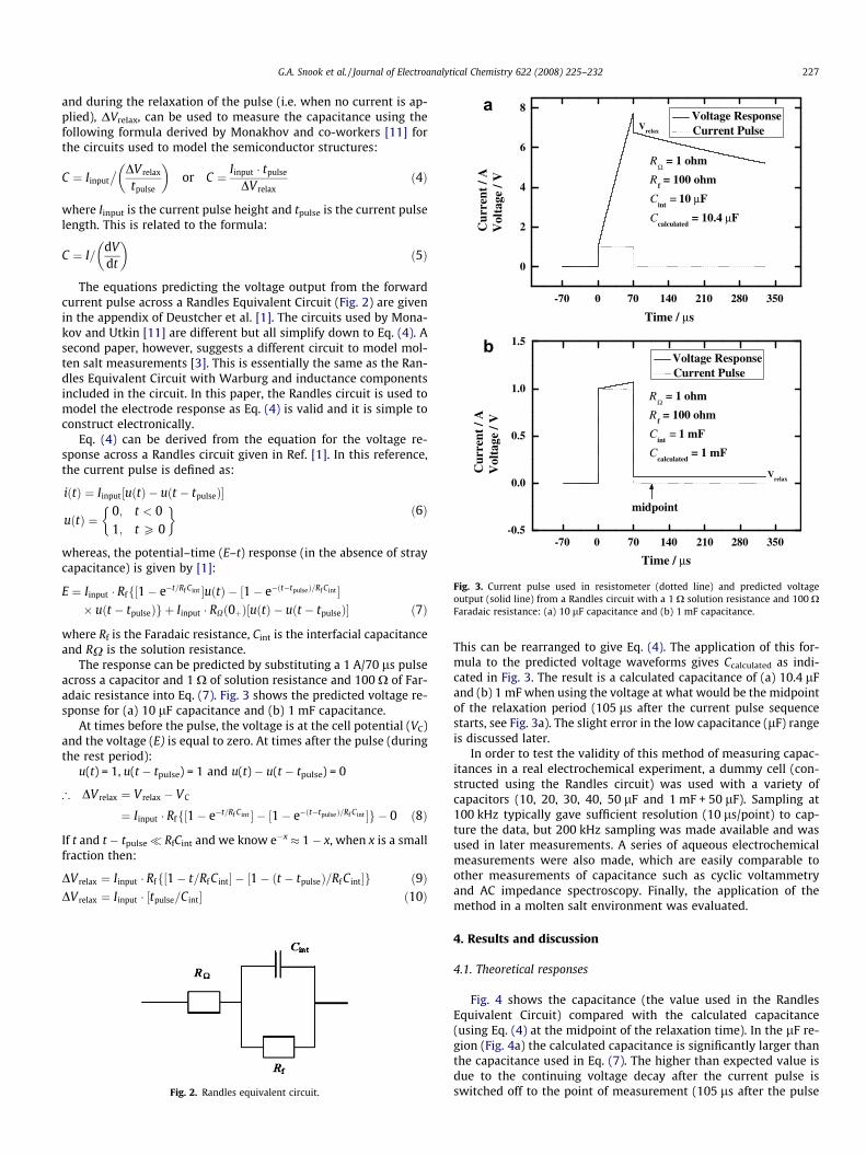
Fig. 3. Current pulse used in resistometer (dotted line) and predicted voltageoutput (solid line) from a Randles circuit with a 1 X solution resistance and 100 XFaradaic resistance: (a) 10 lF capacitance and (b) 1 mF capacitance.

G.A. Snook et al. / Journal of Electroanalytical Chemistry 622 (2008) 225–232 227

and during the relaxation of the pulse (i.e. when no current is ap-plied), DVrelax, can be used to measure the capacitance using thefollowing formula derived by Monakhov and co-workers [11] forthe circuits used to model the semiconductor structures:

C ¼ Iinput� DV relax

tpulse

� �or C ¼ Iinput � tpulse

DV relaxð4Þ

where Iinput is the current pulse height and tpulse is the current pulselength. This is related to the formula:

C ¼ I=dVdt

� �ð5Þ

The equations predicting the voltage output from the forwardcurrent pulse across a Randles Equivalent Circuit (Fig. 2) are givenin the appendix of Deustcher et al. [1]. The circuits used by Mona-kov and Utkin [11] are different but all simplify down to Eq. (4). Asecond paper, however, suggests a different circuit to model mol-ten salt measurements [3]. This is essentially the same as the Ran-dles Equivalent Circuit with Warburg and inductance componentsincluded in the circuit. In this paper, the Randles circuit is used tomodel the electrode response as Eq. (4) is valid and it is simple toconstruct electronically.

Eq. (4) can be derived from the equation for the voltage re-sponse across a Randles circuit given in Ref. [1]. In this reference,the current pulse is defined as:

iðtÞ ¼ Iinput½uðtÞ � uðt � tpulseÞ�

uðtÞ ¼0; t < 01; t P 0

� � ð6Þ

whereas, the potential–time (E–t) response (in the absence of straycapacitance) is given by [1]:

E ¼ Iinput � Rff½1� e�t=Rf Cint �uðtÞ � ½1� e�ðt�tpulseÞ=Rf Cint �� uðt � tpulseÞg þ Iinput � RXð0þÞ½uðtÞ � uðt � tpulseÞ� ð7Þ

where Rf is the Faradaic resistance, Cint is the interfacial capacitanceand RX is the solution resistance.

The response can be predicted by substituting a 1 A/70 ls pulseacross a capacitor and 1 X of solution resistance and 100 X of Far-adaic resistance into Eq. (7). Fig. 3 shows the predicted voltage re-sponse for (a) 10 lF capacitance and (b) 1 mF capacitance.

At times before the pulse, the voltage is at the cell potential (VC)and the voltage (E) is equal to zero. At times after the pulse (duringthe rest period):

u(t) = 1, u(t � tpulse) = 1 and u(t) � u(t � tpulse) = 0

) DV relax ¼ V relax � VC

¼ Iinput � Rff½1� e�t=Rf Cint � � ½1� e�ðt�tpulseÞ=Rf Cint �g � 0 ð8Þ

If t and t � tpulse� RfCint and we know e�x 1 � x, when x is a smallfraction then:

DV relax ¼ Iinput � Rff½1� t=Rf Cint� � ½1� ðt � tpulseÞ=Rf Cint�g ð9ÞDV relax ¼ Iinput � ½tpulse=Cint� ð10Þ

Fig. 2. Randles equivalent circuit.

This can be rearranged to give Eq. (4). The application of this for-mula to the predicted voltage waveforms gives Ccalculated as indi-cated in Fig. 3. The result is a calculated capacitance of (a) 10.4 lFand (b) 1 mF when using the voltage at what would be the midpointof the relaxation period (105 ls after the current pulse sequencestarts, see Fig. 3a). The slight error in the low capacitance (lF) rangeis discussed later.

In order to test the validity of this method of measuring capac-itances in a real electrochemical experiment, a dummy cell (con-structed using the Randles circuit) was used with a variety ofcapacitors (10, 20, 30, 40, 50 lF and 1 mF + 50 lF). Sampling at100 kHz typically gave sufficient resolution (10 ls/point) to cap-ture the data, but 200 kHz sampling was made available and wasused in later measurements. A series of aqueous electrochemicalmeasurements were also made, which are easily comparable toother measurements of capacitance such as cyclic voltammetryand AC impedance spectroscopy. Finally, the application of themethod in a molten salt environment was evaluated.

4. Results and discussion

4.1. Theoretical responses

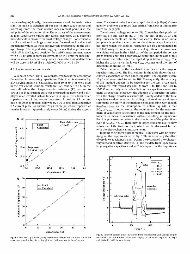
Fig. 4 shows the capacitance (the value used in the RandlesEquivalent Circuit) compared with the calculated capacitance(using Eq. (4) at the midpoint of the relaxation time). In the lF re-gion (Fig. 4a) the calculated capacitance is significantly larger thanthe capacitance used in Eq. (7). The higher than expected value isdue to the continuing voltage decay after the current pulse isswitched off to the point of measurement (105 ls after the pulse

228 G.A. Snook et al. / Journal of Electroanalytical Chemistry 622 (2008) 225–232

sequence begins). Ideally, the measurement should be made the in-stant the pulse is switched off but due to stray capacitances andswitching times the most reliable measurement point is at themidpoint of the relaxation time. The accuracy of the measurementat high capacitance values (mF range) decreases as it becomesmore difficult to measure the small voltage changes. Consequently,small variations in voltage cause larger fluctuations in calculatedcapacitance values, as these are inversely proportional to the volt-age change. The digital data logging means that a precision of�0.3 mV is the highest possible (for a ±10 V measurement rangewith a 16-bit data logger). However, noise will limit the measure-ment to around 2 mV accuracy, which means the limit of detectionwill be close to 35 mF (i.e. (1 A/(0.002 V/70 ls) = 35 mF).

4.2. Randles circuit measurements

A Randles circuit (Fig. 1) was constructed to test the accuracy ofthe method for measuring capacitance. This circuit is shown in Fig.2. A varying amount of capacitance from 10 lF to 1 mF were usedin the test circuit. Solution resistance (RX) was set to 1 X in thetest cell, while the charge transfer resistance (Rf) was set to100 X. The input current pulse was measured separately and is dis-played in an inverted fashion for clarity in Fig. 5. This allows easiersuperimposing of the voltage responses. A positive 1 A currentpulse for 70 ls is applied, followed by a 70 ls rest, then a negative1 A current pulse for another 70 ls. These pulses are repeated atregular intervals (approximately every 60 ms) during the experi-

1E-6 1E-5 1E-4 1E-3 0.01 0.11E-6

1E-5

1E-4

1E-3

0.01

0.1

large error2.0 μF cf. 1 μF

Cal

cula

ted

Cap

acit

ance

/ F

Capacitance / F

Exact Calculated

limit of detection~ 35 mF

0 10 20 30 40 500

10

20

30

40

50

Exact Calculated

Cal

cula

ted

Cap

acit

ance

/ μF

Capacitance / μF

Fig. 4. Calculated capacitance (using the theoretical equations) as a function of thecapacitance used in Eq. (8). (a) Log plot and (b) linear plot in the lF region.

ment. The current pulse has a very rapid rise time (<10 ls). Conse-quently, problems due to artifacts arising from slow or limited risetimes are negligible.

The observed voltage response (Fig. 5) matches that predictedfrom Eq. (7) and seen in Fig. 3. Here the plot of the 30 lF and40 lF measurements are omitted for clarity. There is an initialjump in voltage that is consistent for the different capacitance val-ues, from which the solution resistance can be approximated to1 X. Following this rapid increase in voltage, there is a slower riseto a higher voltage. In the initial part of the rest period, the voltagedrops rapidly and then slowly decays with time. In the case of thistest circuit, the value after the rapid drop is taken as Vrelax. Thehigher the capacitance, the lower Vrelax becomes until the limit ofdetection (at around 35 mF).

Table 1 summarizes the calculated capacitance for the range ofcapacitors measured. The final column in the table shows the cal-culated capacitance of each added capacitor. The capacitors were10 lF and were rated to within 10%. Consequently, the accuracyof this method appears to be excellent for the test circuit used.Subsequent tests varied RX and Rf from 1 to 10 X and 100 to1000 X respectively with little effect on the capacitance measure-ment, as expected. Moreover, the addition of a capacitor in serieswith the charge transfer resistance (Rf) simply added to the totalcapacitance value measured. According to these dummy cell mea-surements the utility of the method is still applicable even thoughRohmCint > tpulse as the assumption to obtain Eq. (4) is thatRfCint tpulse. In other words, the requirement for the measure-ment of capacitance is the same as the requirement for the resis-tometer to measure resistance without resulting in significantFaradaic processes occurring in the time frame of the pulse. How-ever, if RohmCint > tpulse, there may be other problems due to slowrelaxation of the time constant, which will be discussed furtherwith the electrochemical measurements.

Running the current pulse through a 1 X resistor with no capac-itor gives the response shown in Fig. 6. This is essentially the effectof very low capacitance values. During the rest period the voltage isvery low and negative. Using Eq. (4) and the data from Fig. 6 gives alarge negative capacitance value. This emphasizes the importance

0 300 600 900

-2

-1

0

1

2

3

4

5

6

7

8

Vol

tage

Res

pons

e / V

Time / μs

Ipulse

10 μF20 μF50 μF1 mF

reference pulse

increasingcapacitance

Vrelax

Fig. 5. Inverted current pulse measured from resistometer and voltage outputmeasured across the Randles circuit with varying capacitances (10 lF, 20 lF, 50 lFand 1.05 mF). 100 kHz sample rate.

Table 1Measured capacitances from the Randles circuit using the current pulse method andresistometer output

Nominal capacitance/lF Measured capacitance/lF Incremental capacitance/lF

10 10.6 10.620 20.9 10.330 30.9 10.040 40.8 9.850 51.5 10.71050 1150 1100

The first measurement utilizes a 10 lF capacitor in the circuit as Cint. The next fourmeasurements involve adding an additional 10 lF in parallel to the first 10 lFcapacitor each time and the final measurement has an additional 1 mF capacitoradded in parallel with the previously added capacitors.

0.2

0.4

0.6

0.8

1.0

Ccalculated

= 0.7 mF

Vol

tage

/ V

Cur

rent

/ A

Voltage ResponseCurrent Pulse

1 mF+ 10 μF stray capacitance

G.A. Snook et al. / Journal of Electroanalytical Chemistry 622 (2008) 225–232 229

of recording the voltage response to establish the validity of theresults.

4.3. Stray capacitance

Equations for the presence of stray capacitance (Cs) in parallelwith the solution resistance (or strictly speaking across the entireRandles circuit) are given below [1]:

E ¼ Iinput � Rff½1� e�t=Rf Cint �uðtÞ � ½1� e�ðt�tpulseÞ=Rf Cint �� uðt � tpulseÞg þ Iinput � RXð0þÞf½1� e�t=RXCs �uðtÞ� ½1� e�ðt�tpulseÞ=RXCs �uðt � tpulseÞg ð11Þ

These equations are used to determine whether stray capaci-tance will significantly affect the measurement or how much straycapacitance can be tolerated. Fig. 7a shows the current and corre-sponding voltage response for a 1 X solution resistance and 1 mFcapacitance, with 10 lF stray capacitance calculated using Eq.(11). This is clearly different from Eq. (7) and shown in Fig. 3b.The rise time is finite and the voltage response is more curved.The voltage takes some time to reach the rest voltage. Clearly itis better to take the voltage response at the midpoint of the relax-ation time. For a stray capacitance as high as 10 lF, the measuredcapacitance (using the midpoint value) decreases from 1 mF to0.7 mF. The capacitance measured at the midpoint as a function

0.0 0.2 0.4 0.6 0.8-1.2

-0.8

-0.4

0.0

0.4

0.8

1.2

Vol

tage

Res

pons

e / V

time/ ms

reference pulse

0.99 V(~ 1 ohm)

Fig. 6. Voltage output from a 1 X resistor. Illustration of measurement with littlecapacitance in the system. 200 kHz sample rate.

of the stray capacitance is shown in Fig. 7b. Even at 8 X resistance,a very large stray capacitance of 0.5 lF is needed to alter the resultsubstantially. In a typical electrochemical setup the stray capaci-tance will actually be in the pF range [12]. This means that it is un-likely that stray capacitance will significantly affect thecapacitance from current pulse measurement.

4.4. Aqueous measurements at room temperature

A series of measurements in aqueous solution at open circuitwere performed to investigate whether it is possible to estimatethe relative electrode area exposed to the solution. The measure-ments were performed at room temperature in the three electrodemode with a platinum oversized counter-electrode and a Ag/AgCl(3 M KCl) reference electrode. The voltage response was measuredbetween the working electrode and the reference electrode. Twoelectrode mode measurements (no reference electrode) were alsoperformed and gave very similar results.

The first measurement performed used a glassy carbon diskworking electrode (2 mm diameter) in 3 M KCl(aq). The voltage re-sponse from a 1 A pulse is shown in Fig. 8a, and the capacitancemeasured from the pulse method is calculated to be 20.7 lF. Cyclicvoltammetry measurements of capacitance were also performedfor comparison purposes. Here, the cyclic voltammetry for a purelycapacitive material should give a rectangular current–voltage re-sponse – the forward current (Ifwd) equalling C.dV/dt and the re-verse current (Irev) equalling �C.dV/dt (where dV/dt is the scan

-100 0 100 200 300 400

0.0

Time / μs

midpoint

1E-9 1E-8 1E-7 1E-6 1E-5 1E-4 1E-3 0.01 0.1 1 10 100

0.0

0.2

0.4

0.6

0.8

1.0

1.2

stray capacitance

4 Ω

2 Ω

1 Ω

8 Ω

2μF4μF

1μF

Cal

cula

tedC

apac

itan

ce /

mF

Stray Capacitance / F

0.5 μF

solution resistance

Fig. 7. (a) Theoretical voltage response from Eq. (11) with 10 lF stray capacitance(parallel to the 1 X solution resistor). (b) Effect of stray capacitance on calculationof the capacitance from the pulse measurement using a 1 A, 70 ls current pulse anda 1 mF capacitor.

230 G.A. Snook et al. / Journal of Electroanalytical Chemistry 622 (2008) 225–232

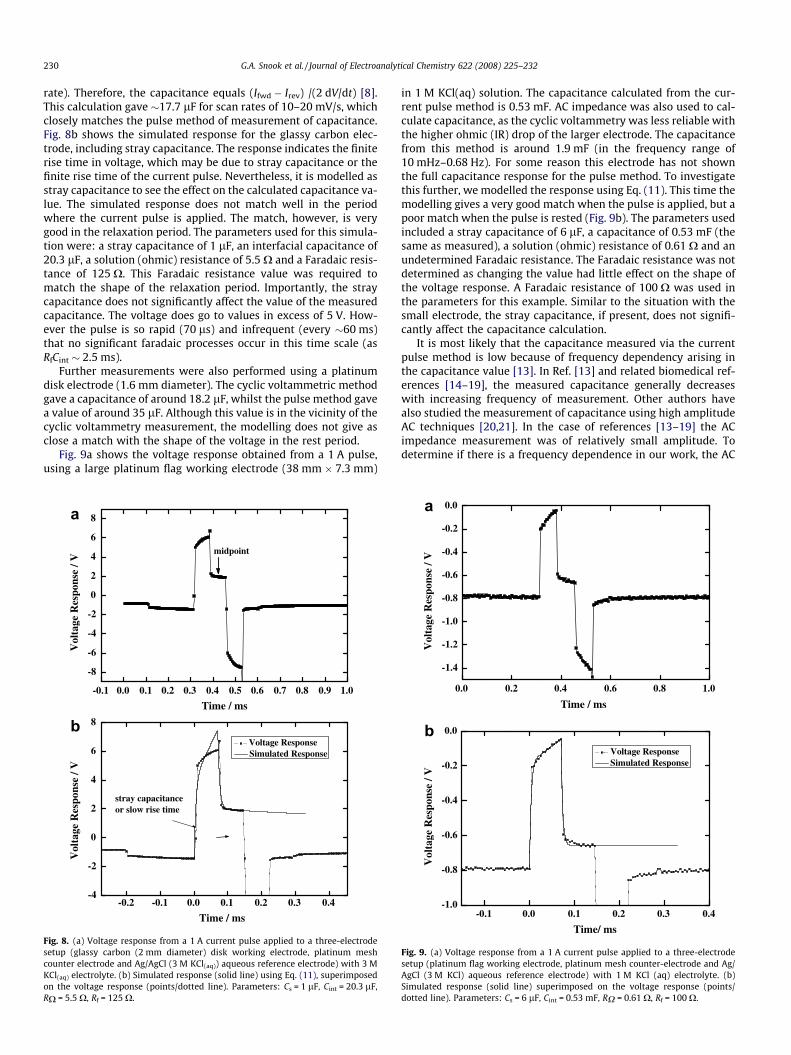
rate). Therefore, the capacitance equals (Ifwd � Irev) /(2 dV/dt) [8].This calculation gave �17.7 lF for scan rates of 10–20 mV/s, whichclosely matches the pulse method of measurement of capacitance.Fig. 8b shows the simulated response for the glassy carbon elec-trode, including stray capacitance. The response indicates the finiterise time in voltage, which may be due to stray capacitance or thefinite rise time of the current pulse. Nevertheless, it is modelled asstray capacitance to see the effect on the calculated capacitance va-lue. The simulated response does not match well in the periodwhere the current pulse is applied. The match, however, is verygood in the relaxation period. The parameters used for this simula-tion were: a stray capacitance of 1 lF, an interfacial capacitance of20.3 lF, a solution (ohmic) resistance of 5.5 X and a Faradaic resis-tance of 125 X. This Faradaic resistance value was required tomatch the shape of the relaxation period. Importantly, the straycapacitance does not significantly affect the value of the measuredcapacitance. The voltage does go to values in excess of 5 V. How-ever the pulse is so rapid (70 ls) and infrequent (every �60 ms)that no significant faradaic processes occur in this time scale (asRfCint � 2.5 ms).

Further measurements were also performed using a platinumdisk electrode (1.6 mm diameter). The cyclic voltammetric methodgave a capacitance of around 18.2 lF, whilst the pulse method gavea value of around 35 lF. Although this value is in the vicinity of thecyclic voltammetry measurement, the modelling does not give asclose a match with the shape of the voltage in the rest period.

Fig. 9a shows the voltage response obtained from a 1 A pulse,using a large platinum flag working electrode (38 mm � 7.3 mm)

-0.1 0.0 0.1 0.2 0.3 0.4 0.5 0.6 0.7 0.8 0.9 1.0

-8

-6

-4

-2

0

2

4

6

8

Vol

tage

Res

pons

e / V

Time / ms

midpoint

-0.2 -0.1 0.0 0.1 0.2 0.3 0.4-4

-2

0

2

4

6

8

Vol

tage

Res

pons

e / V

Time / ms

Voltage Response Simulated Response

stray capacitanceor slow rise time

Fig. 8. (a) Voltage response from a 1 A current pulse applied to a three-electrodesetup (glassy carbon (2 mm diameter) disk working electrode, platinum meshcounter electrode and Ag/AgCl (3 M KCl(aq)) aqueous reference electrode) with 3 MKCl(aq) electrolyte. (b) Simulated response (solid line) using Eq. (11), superimposedon the voltage response (points/dotted line). Parameters: Cs = 1 lF, Cint = 20.3 lF,RX = 5.5 X, Rf = 125 X.

in 1 M KCl(aq) solution. The capacitance calculated from the cur-rent pulse method is 0.53 mF. AC impedance was also used to cal-culate capacitance, as the cyclic voltammetry was less reliable withthe higher ohmic (IR) drop of the larger electrode. The capacitancefrom this method is around 1.9 mF (in the frequency range of10 mHz–0.68 Hz). For some reason this electrode has not shownthe full capacitance response for the pulse method. To investigatethis further, we modelled the response using Eq. (11). This time themodelling gives a very good match when the pulse is applied, but apoor match when the pulse is rested (Fig. 9b). The parameters usedincluded a stray capacitance of 6 lF, a capacitance of 0.53 mF (thesame as measured), a solution (ohmic) resistance of 0.61 X and anundetermined Faradaic resistance. The Faradaic resistance was notdetermined as changing the value had little effect on the shape ofthe voltage response. A Faradaic resistance of 100 X was used inthe parameters for this example. Similar to the situation with thesmall electrode, the stray capacitance, if present, does not signifi-cantly affect the capacitance calculation.

It is most likely that the capacitance measured via the currentpulse method is low because of frequency dependency arising inthe capacitance value [13]. In Ref. [13] and related biomedical ref-erences [14–19], the measured capacitance generally decreaseswith increasing frequency of measurement. Other authors havealso studied the measurement of capacitance using high amplitudeAC techniques [20,21]. In the case of references [13–19] the ACimpedance measurement was of relatively small amplitude. Todetermine if there is a frequency dependence in our work, the AC

0.0 0.2 0.4 0.6 0.8 1.0

-1.4

-1.2

-1.0

-0.8

-0.6

-0.4

-0.2

0.0

Vol

tage

Res

pons

e / V

Time / ms

-0.1 0.0 0.1 0.2 0.3 0.4-1.0

-0.8

-0.6

-0.4

-0.2

0.0

Vol

tage

Res

pons

e / V

Time/ ms

Voltage ResponseSimulated Response

Fig. 9. (a) Voltage response from a 1 A current pulse applied to a three-electrodesetup (platinum flag working electrode, platinum mesh counter-electrode and Ag/AgCl (3 M KCl) aqueous reference electrode) with 1 M KCl (aq) electrolyte. (b)Simulated response (solid line) superimposed on the voltage response (points/dotted line). Parameters: Cs = 6 lF, Cint = 0.53 mF, RX = 0.61 X, Rf = 100 X.

G.A. Snook et al. / Journal of Electroanalytical Chemistry 622 (2008) 225–232 231

impedance data was investigated in the frequency range equiva-lent to the pulse measurement time. If the total time of the signalis 210 ls, the equivalent frequency is around 4750 Hz. So, if weplot imaginary impedance versus 1/(2pf), in the frequency rangeabove around 4000 Hz, we should get an inverse slope equal tothe high frequency capacitance. This measurement has been donefor conducting polymers, in the low frequency range, to give thelow frequency capacitance values [8,9,22–24]. In this previouswork, a knee frequency is identified below which the imaginaryimpedance is purely capacitive (low frequency capacitance region)and above which the imaginary impedance is more complicated.As these conducting polymer materials have relatively slow react-ing capacitances [25] (knee frequencies in the Hz range abovewhich the capacitance behaviour is complicated), the usefulnessof applying this technique to these systems may be limited. Inthe case of the platinum flag electrode, we obtain a capacitanceof around 0.405 ± 0.018 mF in the linear part of the high frequencyimpedance (see Fig. 10). This compares reasonably to the pulsemeasurement of 0.53 mF and indicates it is most likely at thesehigh capacitances in aqueous electrolyte that the capacitance isrelatively slow reacting. This frequency dependence consequentlygives a lower calculated capacitance. The slow relaxation of theRX Cint time constant at these high capacitances (i.e. where thetime constant is greater than 70 ls) appears to affect the resultand introduce a frequency dependence. Also at the high currentsused the cell geometry is likely to be important. The RC time con-stant could be different for different locations on the workingelectrode.

Without proper impedance analysis it is difficult to assign thisnumber as capacitance. It may indeed be a more complicated re-sponse such as that exhibited by a constant phase element. None-theless, good correlation with the measurement and capacitiveproperties such as area of electrode exposed are obtained throughthis method. Simple equivalent circuit modelling (utilizing the Z-View software on the Solartron) using the Randles circuit for fre-quencies between 1 and 15,000 Hz gives reasonable match withthe data (v2 = 0.0463). Better fit is obtained using a constant phaseelement in the place of the capacitor for frequencies between 0.01and 15,000 Hz (v2 = 0.00232). However, the fitted parameter CPE-Pis close to 1 (at 0.914) indicating the behaviour of the constantphase element is close to that of a simple capacitor. An epoxysheathed carbon rod (16.7 mm long and 6.6 mm diameter) elec-trode gave a low frequency AC impedance (10 mHz– 4 Hz) valueof 1.61 mF but a current pulse measurement of 0.205 mF. This timethe high frequency capacitance is 0.257 ± 0.007 mF (�4000–14,000 Hz). Again this matches well with the pulse measurementof capacitance at high frequency.

1 2 3 4 5

-0.02

0.00

0.02

0.04

0.06

0.08

0.10

-Z"

/ ohm

1 / 2π f X 10-5 rad s-1

3830 Hz

14700 Hz

C = 0.405 mF

Fig. 10. High frequency AC impedance data (for the cell in Fig. 9) plotted as – Z00 vs.1/(2pf) in the frequency range of �4000–14,000 Hz. The dotted line indicates thelinear high frequency range from which the capacitance (0.405 mF) is calculated.

These aqueous measurements suggest that care needs to be ta-ken when considering the absolute capacitance value from thistechnique. It is most likely that this capacitance measurementfrom the current pulse could be used mostly for observation ofcapacitance phenomena rather than absolute measurement ofcapacitance. Stray capacitance, however, does not appear to intro-duce additional errors. Connecting the same equipment and datalogger to the dummy cell the capacitance is calculated within10% error. This shows that stray capacitance in the equipmentand leads is not a problem. An interesting test as to whether themethod is giving the right phenomena is to raise and lower theplatinum flag in and out of the aqueous solution. Here the capaci-tance lowers and increases according to the decrease and increasein area of electrode exposed to the electrolyte. Similar types ofexperiments are attempted in molten salts in the next sectionand allow the relative area of electrode exposed to be monitoredduring an experiment.

4.5. Molten salt measurements at high temperature

Using a CaCl2 bath (950 �C) and an oversized pasted titaniacathode (�40 g), the effect of dipping a copper anode to differentdepths into the molten salt bath was investigated. If the titaniaelectrode is sufficiently oversized, the capacitance should bemainly from the anode. This is due to the series connection ofthe anode (CA) and cathode (CC) giving a total capacitance (CT) of

1CT¼ 1

CCþ 1

CAð12Þ

So if CC is sufficiently large compared with CA then the totalcapacitance CT is roughly equal to CA.

This means that, if the rod is dipped to different depths, thecapacitance measured should scale with the depth of the dip (d)as the area exposed to the electrolyte will scale linearly with thedepth (see Eq. (13).

A ¼ pr2 þ dð2prÞ ð13Þ

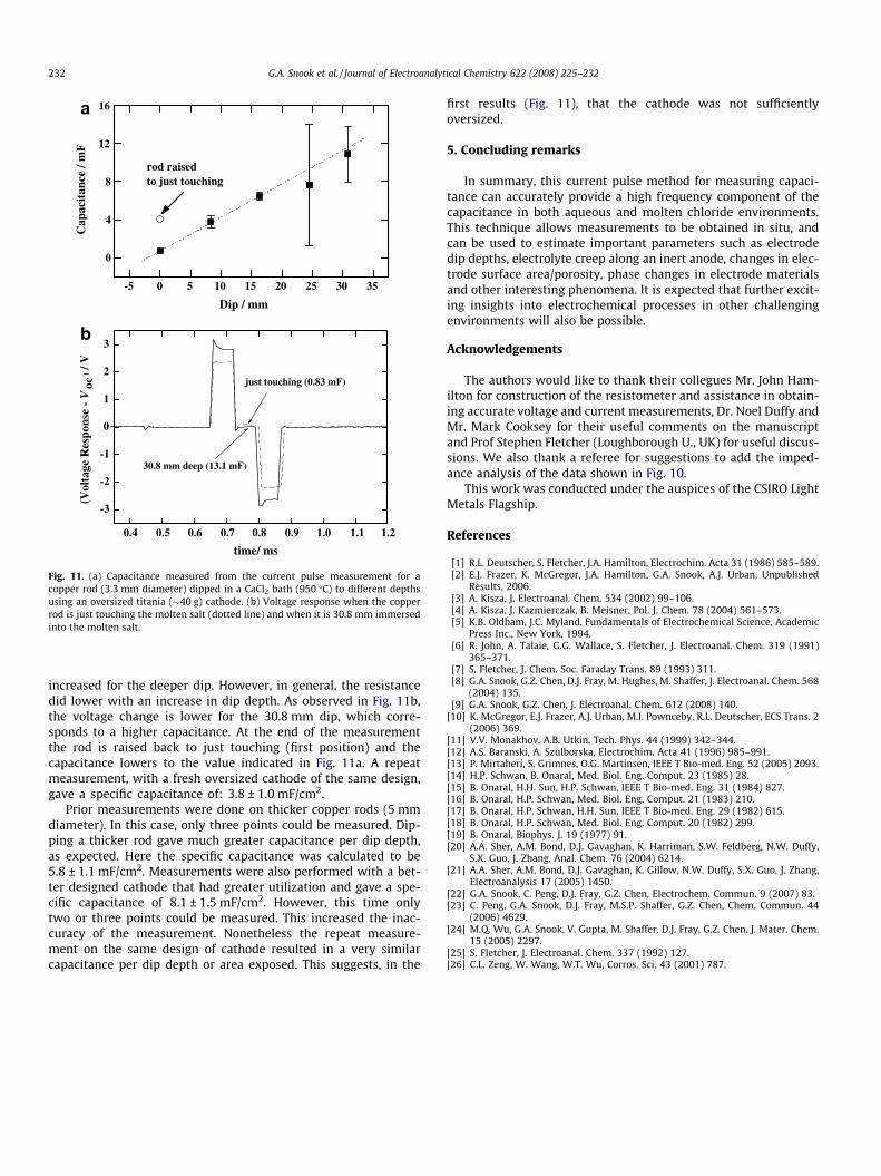
where A is the area, r is the radius of the rod (1.65 mm).Fig. 11 shows the linear relationship between the pulse mea-

sured capacitance and the dip depth. The first point on the graph(just touching the rod in the bath) is determined using the resis-tometer. The point at which the resistance changes from a valueout of the measurement range to a value below 10 X is deter-mined as roughly when the rod is touching the electrolyte (i.e.dip = 0 mm). The points after this are determined by markingon the top of the rod, near the furnace port, each time the rodis lowered and later measuring the separation of these points.In the aqueous electrolyte results, the data logger collects 20 sig-nals and averages these into a resultant average signal. However,in these (earlier measured) molten salt tests, 20 signals are cap-tured one after the other and the data is processed post-collec-tion by manual calculation. The errors given in the graph arefrom the calculated standard deviation from these 20 collectedsignals. There was a problem with the �25 mm measurement(possibly a connection problem) which gave a large error. How-ever, this result was retained to show that the measurementcan give estimates as to the error and indicate when there areproblems with the measurement. Using the updated method ofaveraging the signals will minimize such problems. Using thecalculated area and the capacitance value, the copper was foundto have a specific capacitance of 3.5 ± 0.4 mF/cm2 (assuming thetitania is sufficiently oversized). This compares well with theexample of platinum in molten (Li/K)2CO3 of 4.13 mF/cm2 mea-sured using AC impedance [26]. The voltage response is shownin Fig. 11b. Strangely, the resistance in this example has

-5 0 5 10 15 20 25 30 35

0

4

8

12

16

Cap

acit

ance

/ m

F

Dip / mm

rod raisedto just touching

0.4 0.5 0.6 0.7 0.8 0.9 1.0 1.1 1.2

-3

-2

-1

0

1

2

3

30.8 mm deep (13.1 mF)

(Vol

tage

Res

pons

e -

Voc

)/ V

time/ ms

just touching (0.83 mF)

Fig. 11. (a) Capacitance measured from the current pulse measurement for acopper rod (3.3 mm diameter) dipped in a CaCl2 bath (950 �C) to different depthsusing an oversized titania (�40 g) cathode. (b) Voltage response when the copperrod is just touching the molten salt (dotted line) and when it is 30.8 mm immersedinto the molten salt.

232 G.A. Snook et al. / Journal of Electroanalytical Chemistry 622 (2008) 225–232

increased for the deeper dip. However, in general, the resistancedid lower with an increase in dip depth. As observed in Fig. 11b,the voltage change is lower for the 30.8 mm dip, which corre-sponds to a higher capacitance. At the end of the measurementthe rod is raised back to just touching (first position) and thecapacitance lowers to the value indicated in Fig. 11a. A repeatmeasurement, with a fresh oversized cathode of the same design,gave a specific capacitance of: 3.8 ± 1.0 mF/cm2.

Prior measurements were done on thicker copper rods (5 mmdiameter). In this case, only three points could be measured. Dip-ping a thicker rod gave much greater capacitance per dip depth,as expected. Here the specific capacitance was calculated to be5.8 ± 1.1 mF/cm2. Measurements were also performed with a bet-ter designed cathode that had greater utilization and gave a spe-cific capacitance of 8.1 ± 1.5 mF/cm2. However, this time onlytwo or three points could be measured. This increased the inac-curacy of the measurement. Nonetheless the repeat measure-ment on the same design of cathode resulted in a very similarcapacitance per dip depth or area exposed. This suggests, in the

first results (Fig. 11), that the cathode was not sufficientlyoversized.

5. Concluding remarks

In summary, this current pulse method for measuring capaci-tance can accurately provide a high frequency component of thecapacitance in both aqueous and molten chloride environments.This technique allows measurements to be obtained in situ, andcan be used to estimate important parameters such as electrodedip depths, electrolyte creep along an inert anode, changes in elec-trode surface area/porosity, phase changes in electrode materialsand other interesting phenomena. It is expected that further excit-ing insights into electrochemical processes in other challengingenvironments will also be possible.

Acknowledgements

The authors would like to thank their collegues Mr. John Ham-ilton for construction of the resistometer and assistance in obtain-ing accurate voltage and current measurements, Dr. Noel Duffy andMr. Mark Cooksey for their useful comments on the manuscriptand Prof Stephen Fletcher (Loughborough U., UK) for useful discus-sions. We also thank a referee for suggestions to add the imped-ance analysis of the data shown in Fig. 10.

This work was conducted under the auspices of the CSIRO LightMetals Flagship.

References

[1] R.L. Deutscher, S. Fletcher, J.A. Hamilton, Electrochim. Acta 31 (1986) 585–589.[2] E.J. Frazer, K. McGregor, J.A. Hamilton, G.A. Snook, A.J. Urban, Unpublished

Results, 2006.[3] A. Kisza, J. Electroanal. Chem. 534 (2002) 99–106.[4] A. Kisza, J. Kazmierczak, B. Meisner, Pol. J. Chem. 78 (2004) 561–573.[5] K.B. Oldham, J.C. Myland, Fundamentals of Electrochemical Science, Academic

Press Inc., New York, 1994.[6] R. John, A. Talaie, G.G. Wallace, S. Fletcher, J. Electroanal. Chem. 319 (1991)

365–371.[7] S. Fletcher, J. Chem. Soc. Faraday Trans. 89 (1993) 311.[8] G.A. Snook, G.Z. Chen, D.J. Fray, M. Hughes, M. Shaffer, J. Electroanal. Chem. 568

(2004) 135.[9] G.A. Snook, G.Z. Chen, J. Electroanal. Chem. 612 (2008) 140.

[10] K. McGregor, E.J. Frazer, A.J. Urban, M.I. Pownceby, R.L. Deutscher, ECS Trans. 2(2006) 369.

[11] V.V. Monakhov, A.B. Utkin, Tech. Phys. 44 (1999) 342–344.[12] A.S. Baranski, A. Szulborska, Electrochim. Acta 41 (1996) 985–991.[13] P. Mirtaheri, S. Grimnes, O.G. Martinsen, IEEE T Bio-med. Eng. 52 (2005) 2093.[14] H.P. Schwan, B. Onaral, Med. Biol. Eng. Comput. 23 (1985) 28.[15] B. Onaral, H.H. Sun, H.P. Schwan, IEEE T Bio-med. Eng. 31 (1984) 827.[16] B. Onaral, H.P. Schwan, Med. Biol. Eng. Comput. 21 (1983) 210.[17] B. Onaral, H.P. Schwan, H.H. Sun, IEEE T Bio-med. Eng. 29 (1982) 615.[18] B. Onaral, H.P. Schwan, Med. Biol. Eng. Comput. 20 (1982) 299.[19] B. Onaral, Biophys. J. 19 (1977) 91.[20] A.A. Sher, A.M. Bond, D.J. Gavaghan, K. Harriman, S.W. Feldberg, N.W. Duffy,

S.X. Guo, J. Zhang, Anal. Chem. 76 (2004) 6214.[21] A.A. Sher, A.M. Bond, D.J. Gavaghan, K. Gillow, N.W. Duffy, S.X. Guo, J. Zhang,

Electroanalysis 17 (2005) 1450.[22] G.A. Snook, C. Peng, D.J. Fray, G.Z. Chen, Electrochem. Commun. 9 (2007) 83.[23] C. Peng, G.A. Snook, D.J. Fray, M.S.P. Shaffer, G.Z. Chen, Chem. Commun. 44

(2006) 4629.[24] M.Q. Wu, G.A. Snook, V. Gupta, M. Shaffer, D.J. Fray, G.Z. Chen, J. Mater. Chem.

15 (2005) 2297.[25] S. Fletcher, J. Electroanal. Chem. 337 (1992) 127.[26] C.L. Zeng, W. Wang, W.T. Wu, Corros. Sci. 43 (2001) 787.