CURVATURE MATTER COUPLING: SOME

COSMIC ASPECTS

By

Muhammad Zubair

A THESIS

SUBMITTED IN PARTIAL FULFILLMENT OF THE

REQUIREMENTS FOR THE DEGREE OF

DOCTOR OF PHILOSOPHY

IN

MATHEMATICS

Supervised By

Prof. Dr. Muhammad Sharif

UNIVERSITY OF THE PUNJAB

LAHORE-PAKISTAN

DECEMBER, 2013

CERTIFICATE

I certify that the research work presented in this thesis is

the original work of Mr. Muhammad Zubair S/O Mehboob

Ahmed and is carried out under my supervision. I endorse its

evaluation for the award of Ph.D. degree through the official

procedure of University of the Punjab.

Prof. Dr. Muhammad Sharif(Supervisor)

ii

DECLARATION

I, Mr. Muhammad Zubair S/O Mehboob Ahmed,

hereby declare that the matter printed in this thesis is my

original work. This thesis does not contain any material that

has been submitted for the award of any other degree in any

university and to the best of my knowledge, neither does this

thesis contain any material published or written previously by

any other person, except due reference is made in the text of

this thesis.

Muhammad Zubair

iii

DEDICATED

To

My Loving Parents

iv

Table of Contents

Table of Contents v

List of Figures vii

Abstract ix

Acknowledgements xi

Notations xiii

Introduction 1

1 Modified Gravities and Their Implications 6

1.1 Modified Gravitational Theories . . . . . . . . . . . . . . . . 7

1.1.1 Theories Involving Non-Minimal Coupling . . . . . . 8

1.1.2 f(R, T ) Gravity . . . . . . . . . . . . . . . . . . . . . 8

1.1.3 f(R, T,Q) Gravity . . . . . . . . . . . . . . . . . . . 11

1.2 Stability Criteria . . . . . . . . . . . . . . . . . . . . . . . . 12

1.3 Thermodynamics . . . . . . . . . . . . . . . . . . . . . . . . 14

1.3.1 Zeroth Law . . . . . . . . . . . . . . . . . . . . . . . 14

1.3.2 First Law . . . . . . . . . . . . . . . . . . . . . . . . 15

1.3.3 Second Law . . . . . . . . . . . . . . . . . . . . . . . 15

1.3.4 Third Law . . . . . . . . . . . . . . . . . . . . . . . . 16

1.4 Laws of BH Dynamics or Thermodynamics . . . . . . . . . . 17

1.4.1 Zeroth Law . . . . . . . . . . . . . . . . . . . . . . . 17

1.4.2 First Law . . . . . . . . . . . . . . . . . . . . . . . . 18

1.4.3 Second Law . . . . . . . . . . . . . . . . . . . . . . . 18

1.4.4 Generalized Second Law . . . . . . . . . . . . . . . . 19

1.4.5 Thermal Equilibrium . . . . . . . . . . . . . . . . . . 21

1.4.6 Third Law . . . . . . . . . . . . . . . . . . . . . . . . 21

1.5 Energy Conditions . . . . . . . . . . . . . . . . . . . . . . . 21

1.6 Anisotropic Cosmologies . . . . . . . . . . . . . . . . . . . . 24

v

1.7 Cosmological Parameters . . . . . . . . . . . . . . . . . . . . 26

1.7.1 Hubble’s Law and Hubble Parameter . . . . . . . . . 26

1.7.2 Mean and Directional Hubble Parameters . . . . . . 27

1.7.3 Anisotropy Parameter of Expansion . . . . . . . . . . 28

1.7.4 Deceleration Parameter . . . . . . . . . . . . . . . . . 28

1.8 The Expansion and Shear Scalar . . . . . . . . . . . . . . . . 29

2 Thermodynamics Laws in f(R, T ) and f(R, T,Q) Modified

Theories 30

2.1 Thermodynamics in f(R, T ) Gravity . . . . . . . . . . . . . 31

2.1.1 First Law of Thermodynamics . . . . . . . . . . . . . 33

2.1.2 Generalized Second Law of Thermodynamics . . . . . 35

2.2 Redefining the Dark Components . . . . . . . . . . . . . . . 37

2.2.1 First Law of Thermodynamics . . . . . . . . . . . . . 39

2.2.2 Generalized Second Law of Thermodynamics . . . . . 41

2.3 Thermodynamics in f(R, T,Q) Gravity . . . . . . . . . . . . 42

2.3.1 First Law of Thermodynamics . . . . . . . . . . . . . 44

2.3.2 Generalized Second Law of Thermodynamics . . . . . 48

3 Energy Conditions Constraints and Stability of f(R, T ) and

f(R, T,Q) Modified Theories 56

3.1 Energy Conditions in f(R, T,Q) Gravity . . . . . . . . . . . 57

3.2 Constraints on Class of f(R, T,Q) Models . . . . . . . . . . 63

3.2.1 f(R, T,Q) = R + αQ . . . . . . . . . . . . . . . . . . 63

3.2.2 f(R, T,Q) = R(1 + αQ) . . . . . . . . . . . . . . . . 65

3.3 Energy Conditions in f(R, T ) Gravity . . . . . . . . . . . . . 67

3.3.1 Power Law Solutions . . . . . . . . . . . . . . . . . . 72

3.4 Stability of Power Law Solutions . . . . . . . . . . . . . . . 80

3.4.1 f(R, T ) = f(R) + λT . . . . . . . . . . . . . . . . . . 80

3.4.2 f(R, T ) = R + 2f(T ) . . . . . . . . . . . . . . . . . . 82

4 Anisotropic Universe Models in f(R, T ) Gravity 84

4.1 f(R, T ) Gravity and Bianchi I Universe . . . . . . . . . . . . 85

4.2 Solution of the Field Equations . . . . . . . . . . . . . . . . 86

4.2.1 Exponential Expansion Model . . . . . . . . . . . . . 88

4.2.2 Power Law Expansion Model . . . . . . . . . . . . . 91

4.3 Massless Scalar Field Models . . . . . . . . . . . . . . . . . . 95

4.4 Solutions for Fixed Anisotropy Parameter . . . . . . . . . . 97

5 Discussion and Conclusion 104

Bibliography 117

vi

List of Figures

2.1 Evolution of GSLT for the Lagrangian f(R, T,Q) = R+αQ,

the left panel shows the bound on m for α = −2 whereas in

the right panel we set m = 10. It is evident that GSLT is

valid only if α < 0, m > 1. . . . . . . . . . . . . . . . . . . . 53

2.2 Evolution of GSLT for the Lagrangian f(R, T,Q) = R(1 +

αQ), the left panel shows constraint on m for α = 10 whereas

in the right panel, we set m = 10. It is evident that GSLT

is valid only if α > 0, m > 1. . . . . . . . . . . . . . . . . . . 54

2.3 Evolution of GSLT for the Lagrangian f(R, T,Q) = R +

f(Q) + g(T ), the left panel shows constraints on parameters

C and D for z = 0 whereas in the right panel, we set Ci and

Di in terms of unique parameter Υ and constrain the values

of Υ. We choose H0 = 67.3, Ωm0 = 0.315 from the recent

Planck results [33]. . . . . . . . . . . . . . . . . . . . . . . . 55

4.1 Evolution of ∆ versus t for different values of n. We set

l = 0.1, k = 3, and α = 0.05. . . . . . . . . . . . . . . . . . . 89

4.2 Evolution of NEC for n = 2. The left graph shows that NEC

is satisfied for α < 0 and it is violated for α > 0 at the right

side. We set l = λ = 0.1 and k = 3. . . . . . . . . . . . . . . 90

4.3 The left graph shows the behavior of ρ for −6 < n ≤ 0 and

n < −6, while the right graph presents the evolution of ρ for

n > 0. We set l = λ = 0.1, k = 3 and α = 0.05. . . . . . . . 91

vii

4.4 Plot of ∆ versus t for different values of n. We set l = 0.1,

k = c2 = 3, m = 0.9 and α = 0.05. . . . . . . . . . . . . . . . 92

4.5 Behavior of NEC versus α for n = 3. The left part shows

that NEC is satisfied for α < 0, while it is violated for α > 0

shown on the right side. We set l = λ = 0.1, k = c2 = 3 and

m = 0.9. . . . . . . . . . . . . . . . . . . . . . . . . . . . . . 93

4.6 This figure is plotted for n = 2. The left part shows that

NEC is violated for α < 0, whereas NEC is satisfied for

α > 0 shown on right side. . . . . . . . . . . . . . . . . . . . 94

4.7 Evolution of ρ versus t for n ≥ 0. We set l = λ = 0.1,

k = c2 = 3, m = 0.9 and α = 0.05. . . . . . . . . . . . . . . . 95

4.8 Evolution of φ versus t for m = 0 and different values of

n: solid(black) n = 1; dashed(red), n = 0; dahsed(blue),

n = −1. We set l = λ = 0.1, k = 3 and α = 0.05. . . . . . . 96

4.9 Evolution of φ versus t for m 6= 0 and different values of

n: solid(black) n = 1; dashed(red), n = 0; dahsed(blue),

n = −1. We set l = λ = 0.1, k = c2 = 3, m = 0.9 and

α = 0.05. . . . . . . . . . . . . . . . . . . . . . . . . . . . . . 97

4.10 Evolution of NEC for exponential model. The NEC is vio-

lated for (a) λ > 0 whereas it can be satisfied for (b) λ < −25.

We set χ = 3, l = c1 = 0.1 and γ = 0.001. . . . . . . . . . . 99

4.11 Plot of energy density corresponding to different values of

coupling parameter. . . . . . . . . . . . . . . . . . . . . . . . 99

4.12 Evolution of NEC for power law model. Plot (a) shows that

NEC is violated for λ > −25 which favors the accelerated

expansion. It can be met for λ < −25 as shown in plot (b). . 101

4.13 Evolution of NEC for 0 < m < 1 with λ = 10. For λ < −25,

we have ρ + p > 0. . . . . . . . . . . . . . . . . . . . . . . . 102

4.14 Evolution of ρ for power law model. In plot (a) we set m =

0.9 and −10 < λ < 10 whereas in plot (b) we vary m in the

range of phantom evolution and set λ = 0.1 . . . . . . . . . 102

viii

Abstract

This thesis studies some cosmic aspects in modified theories involving cur-

vature matter coupling. In this setting, we concentrate on f(R, T ) and

f(R, T, RµνTµν) theories to discuss the thermodynamic laws with the non-

equilibrium description at the apparent horizon of FRW universe. It is

shown that Friedmann equations can be transformed to the form of Clau-

sius relation ThSeff = δQ, Seff is the entropy which contains contributions

both from horizon entropy as well as additional entropy term introduced

due to the non-equilibrating description and δQ is the energy flux across

the horizon. The generalized second law of thermodynamics is also estab-

lished in a more comprehensive form and one can recover the corresponding

results in Einstein as well as f(R) theories. We remark that equilibrium

description in such theories needs more study to follow.

Moreover, we discuss the validity of energy conditions in f(R, T,RµνTµν)

gravity. The corresponding energy conditions are presented in terms of re-

cent values of Hubble, deceleration, jerk and snap parameters. In particular,

we use two specific models recently developed in literature to study concrete

application of these conditions as well as Dolgov-Kawasaki instability. We

explore f(R, T ) gravity as a specific case to this modified theory for expo-

nential and power law models. The exact power law solutions are obtained

for two particular cases in homogeneous and isotropic f(R, T ) cosmology.

Finally, we find certain constraints which have to be satisfied to ensure that

power law solutions may be stable and match the bounds prescribed by the

energy conditions.

We also explore the locally rotationally symmetric Bianchi type I model

ix

x

with perfect fluid as matter content in f(R, T ) gravity. The exact solutions

of the field equations are obtained for two expansion laws namely exponen-

tial and power law expansions. The physical and kinematical quantities are

examined for both cases in future evolution of the universe. We investigate

the validity of null energy condition and conclude that our solutions are

consistent with the current observations.

Acknowledgements

All praises and thanks to Almighty Allah, Who (Alone) created the heavens

and the earth, and prevailed the darkness and sparked the light. I owe my

deep gratitude to Him, Who endowed me with opportunity, knowledge,

patience and potential to impart a drop, in the sea of knowledge. All

praise and best regards to the Holy Prophet Hazrat Muhammad (PBUH),

the mercy on mankind, who is the greatest inspiration for all knowledge

seekers.

One of the joys of this completion is to look over the past journey and

remember all the friends and family who have helped and supported me

along this long but fulfilling road. This thesis has been kept on track and

seen through to completion with the support and encouragement of numer-

ous people. I would like to thank all those who made this thesis possible

and an unforgettable experience for me.

First and foremost, I feel great pleasure to express my heartiest gratitude

and deep sense of obligation to my distinguished supervisor and chairman

Prof. Dr. Muhammad Sharif for every bit of guidance, assistance,

expertise, enthusiasm and constructive criticism. Sir! you have been a

tremendous mentor for me and I feel extremely privileged to have worked

under your supervision. I am grateful to Department of Mathematics for

providing the research facilities and Higher Education Commission, Islam-

abad for its financial support through the Indigenous Ph.D. 5000 Fellowship

Program Batch-VII.

I want to express my deeply felt thanks to all faculty members and wor-

thy school as well as college teachers especially Assoc. Prof. Aslam Malik,

Mr. Daud Ahmed, Mr. M. Riaz, Dr. Aziz Ullah, Prof. Shahid Siddiqi, Dr.

Ghazala Akram, Mr. Zafar Islam, Prof. Hameed Siddiqi and Prof. Hamid

Shah for their guidance and helping nature. I am obliged to Prof. Asghar

xi

xii

Qadir for his valuable suggestions and comments to improve this thesis. I

would also like to acknowledge him with much appreciation for suggesting a

new direction regarding modified theories of gravity. I would like to thank

Prof. Dr. Jin Lin Han and his group members for their warm hospitality

at National Astronomical Observatories, Chinese Academy of Sciences Bei-

jing, during my three months stay. I really enjoyed that period of my life

and it was unforgettable tour with my senior Dr. Abbas. I acknowledge

him for his support in this tour and in my PhD.

It is my pleasure to acknowledge all my PhD fellows especially Mr.

Jawad, Mr. Hamood, Mr. Younis, Mr. Muzammal and my cabin fellow Mr.

M. Azam for their help, cooperative behavior and providing a stimulating

and conducive environment. I would also like to thank my colleague Miss

Saira Waheed for cooperative and supporting attitude. I am obliged to

many people especially Zahid bahi, Advoc. Hafiz Sami, Mr. Shakeel and

Mr. Tariq who in some way contributed to my educational career. I would

particularly thank neurophysician Dr. Mazhar Badshah for his medication

to recover from my brain disease and encouragement to continue my PhD.

I am grateful to all my friends especially Ihtesham Zafar, Haseeb Muzaf-

far, Jawad Ali, Imran Sarwar, ShahRukh, Irtaza, Muqaddar, Zahid and

Quyum for their unflagging love, care and encouragement throughout this

period. I give credit to Ihtesham who always tried to keep us connected and

wanted me to be there in every gathering. I apologize for ignoring them

most of the times because of my occupied schedules. I am ever indebted to

Imran bahi for his valuable support in my whole hostel life.

This acknowledgement will be incomplete without mentioning my feel-

ings with tearful eyes for my loving parents who taught me to take the first

step, to speak the first word and inspired me throughout of my life. My

deepest gratitude goes to my family for their unwearying love and support;

this thesis would have been simply impossible without them. Many special

thanks are due to my sister Rakhshanda for her support in completing my

educational career. My father always encouraged and supported me and

my mother whose hands always arose in prayers for me, she is everything

for me.

Lahore Muhammad Zubair

December, 2013

Notations

In this thesis, the convention to be used for the metric signatures will be

(+,−,−,−) and Greek indices will vary from 0 to 3, if different it will be

mentioned. Also, we shall use the following list of notations and abbrevia-

tions.

AH: Apparent Horizon

BAO: Baryon Acoustic Oscillations

BH: Black Hole

BI: Bianchi Type I

CMB: Cosmic Microwave Background

CMC: Curvature Matter Coupling

DE: Dark Energy

DEC: Dominant Energy Condition

DM: Dark Matter

EoS: Equation of State

FLT: First Law of Thermodynamics

FRW: Friedmann-Roberston-Walker

GR: General Relativity

GSLT: Generalized Second Law of Thermodynamics

ΛCDM: Λ-Cold Dark Matter

LRS: Locally Rotationally Symmetric

MGT: Modified Gravitational Theory

NEC: Null Energy Condition

SEC: Strong Energy Condition

SNeIa: Supernovae Type Ia

WEC: Weak Energy Condition

xiii

Introduction

Humans have been speculating about the Universe in search of reasons to

questions like, how did it come into being and how will it evolve in future?

What is its matter energy contents and how these are structured? Cosmol-

ogy, the study of the cosmos, explains the origin and evolution of entire

cosmic contents, tries to understand the underlying physical processes and

comprehend the laws of physics assumed to hold throughout the cosmos.

Cosmology is ranked among the modern and dynamic physical sciences due

to its progress both in theory and observations. The development of cos-

mology and gravitation can be seen as one of the scientific triumphs of the

twentieth century. In 1998, observations of SNeIa accumulated by the high-

redshift SN team [1] and SN cosmology project team [2] appeared as illumi-

nating candles in disclosing the expansion of the Universe. The source for

this observed cosmic acceleration may be an anonymous energy component

entitled as DE. In spite of tremendous efforts, late cosmic acceleration is

certainly a major challenge for cosmologists. The direct evidence for cosmic

acceleration has strengthened over time with measurements from tempera-

ture anisotropies in CMB [3] and BAO [4] which confirm the existence of

DE.

Contemporary Planck results [5] acquired by ESA’s Planck space tele-

scope predict that cosmos is made of 4.9% baryons, 26.8% DM and 68.3%

1

2

DE which confirms that cosmic energy budget is dominated by DE. Dark

energy is recognized by its distinctive nature from ordinary matter sources

having negative pressure which may lead to cosmic expansion counter strik-

ing the gravitational pull. To explore the properties of DE, one needs to

clarify whether it is Λ or it originates from other dynamical sources. If the

origin of DE is not Λ then one may seek for some other possibilities to count

the cosmic expansion. A useful way to categorize the candidates of DE is

according to how they modify Einstein equations which relate geometry

with energy and matter in cosmic contents. The first proposal is to modify

the matter part in Einstein equations by considering exotic matter source

with a negative pressure [6]. In this proposal, the representative models are

quintessence [7], K-essence [8], phantom field [9] and Chaplygin gas [10].

These dynamical DE models can be distinguished from Λ by defining the

evolution for EoS parameter.

The other proposal for the construction of DE models is the modification

of Einstein-Hilbert action which leads to modified gravity models. Of the

many proposals for modified gravity, we will be interested in f(R) gravity

[11], f(R, T ) gravity [12] and f(R, T,Q) gravity [13, 14], where R is the

scalar curvature, T is the trace of energy-momentum tensor and Q is the

contraction of Ricci tensor and energy momentum tensor. Harko et al. [12]

introduced a matter geometry coupled system in the setting of Lagrangian

f(R, T ), a generic function of R and T . The field equations were formu-

lated for general and some specific forms of Lagrangian in metric formalism.

Alvarenga et al. [15] explored the scalar cosmological perturbations for a

specific model in this theory to guarantee the standard continuity equa-

tion and obtained the matter density perturbed equations. Shabani and

3

Farhoudi [16] discussed the cosmological solutions for three specific cate-

gories in this theory through phase space analysis. Recently, an extension of

f(R, T ) theory is proposed by assuming the non-minimal coupling through

the contraction of Ricci tensor Rαβ as well as Tαβ and resulting action is

refereed as f(R, T,Q) [13, 14]. Haghani et al. [13] developed the field equa-

tions in metric formalism and investigated the cosmological implications for

conserved as well as nonconserved Tαβ. Odinstov and Saez-Gomez [14] re-

constructed this theory for some well-known solutions like de Sitter, power

law and ΛCDM cosmology and discussed the issue of matter instability.

The discovery of black hole thermodynamics set up a significant connec-

tion between gravity and thermodynamics [17, 18]. The Hawking tempera-

ture T = |κsg |2π

, where κsg is the surface gravity, and horizon entropy S = A4G

satisfy FLT. The association of FLT with Einstein equations has been ex-

plored extensively in settings of GR and MGTs. Cai and Kim [19] developed

a connection between FLT at AH with the field equations for the FRW Uni-

verse model. The FRW equations for any spatial curvature are derived using

the relation ThdSh = −dE (Th = 1/2πrA and Sh = πrA/G), where E is the

heat flow across the horizon. Eling et al. [20] realized that thermodynamic

derivation of Einstein equations in f(R) gravity needs a modification to

non-equilibrium setting. In order to get the right equations, it is necessary

to add an extra entropy production term in the Clausius relation to balance

the energy conservation. This corresponds to non-equilibrium description

of thermodynamics. In spite of of these studies, reinterpretation of non-

equilibrium correction has also been explored and alternative treatments

have been suggested. Bamba and Geng [21, 23] suggested that equilibrium

picture of thermodynamics can be established in MGTs by incorporating

4

the extra degrees of freedom in effective Tαβ. They discussed the FLT and

GSLT in both equilibrium and non-equilibrium descriptions.

In GR, the theory of matter is specified on the basis of classical energy

conditions namely, weak, null, strong and dominant conditions which make

certain constraints such as positivity of energy density and dominance of

energy density over pressure [24]. Santos [28] explored the energy conditions

bounds in f(R) gravity and constrained two known models in terms of

recent figured values of deceleration, jerk and snap parameters. This scheme

has been implemented in other MGTs including f(T ) gravity [29], f(G)

gravity [30], scalar-tensor theories [31] and modified gravities with CMC

[32].

This thesis is devoted to look into the cosmological implications of

f(R, T ) and f(R, T,Q) theories of gravity. We address the thermodynamic-

gravity relation and energy conditions bounds on these theories. The exact

solutions are discussed for power law cosmology and anisotropic cosmic

models which assist in reconstructing the corresponding Lagrangian. The

thesis is outlined in the following format.

Chapter One presents an overview of the current results concerning

the dynamics of cosmos and indications for the modification of GR. We

briefly introduce modified theories involving CMC and their corresponding

formalisms.

Chapter Two deals with the study of thermodynamic laws in the frame-

work of f(R, T ) and f(R, T,Q) gravities. We establish the FLT and GSLT

at the AH of FRW spacetime in non-equilibrium picture of thermodynamics.

The validity of GSLT is examined for two particular models by constraining

the coupling parameters. We also investigate the existence of equilibrium

5

description of thermodynamics for these theories.

Chapter Three presents the picture of energy conditions constraints in

the configuration of FRW spacetime for f(R, T ) and f(R, T,Q) gravities.

The corresponding inequalities are obtained in terms of recent values of

Hubble, deceleration, jerk and snap parameters which can reduce to well-

known results in GR and f(R) gravity. The exact power law solutions in

f(R) gravity are constrained against the energy conditions and linear ho-

mogeneous perturbations. We also consider two specific forms of f(R, T,Q)

gravity to develop concrete application of these conditions as well as Dolgov-

Kawasaki instability.

Chapter Four is devoted to discuss the LRS BI model with matter con-

tent as perfect fluid in f(R, T ) gravity. The exact solutions of the field equa-

tions are obtained for two expansion laws namely exponential and power

law expansions. We check the validity of NEC and conclude that these

solutions favor the phantom model. We also establish the functional forms

of Lagrangian for both dynamical and constant anisotropy parameters.

Chapter Five comprises of concluding remarks and suggests some issues

requiring further consideration.

Chapter 1

Modified Gravities and TheirImplications

The most significant characteristic of our cosmos is its large scale homogene-

ity and isotropy, the so called Cosmological Principle which is considered as

the cornerstone of modern cosmology. According to this principle at each

epoch, the Universe represents the same aspect from every point, except

for local irregularities. In fact, there is no privileged direction or position

in the Universe. Following this idea, the line element of homogeneous and

isotropic FRW spacetime is given by

ds2 = dt2 − a2(t)[dr2

1− kr2+ r2dθ2 + r2 sin2 θdφ2], (1.0.1)

where k = +1,−1, 0 corresponds to closed, open and flat geometries, re-

spectively.

In this chapter, we present the candidates of MGTs involving matter

geometry coupling and overview thermodynamic laws, energy conditions

and some other cosmological components.

6

7

1.1 Modified Gravitational Theories

Modified gravitational theories have been the subject of great interest in

cosmology and provide a convincing way for settling the issue of late-time

acceleration. The concept that gravity is not described precisely by GR

but rather by some alternative theories has been viewed under different cir-

cumstances. There are various ways to modify GR incorporating quadratic

Lagrangian, consisting of second order curvature invariants such as R2,

RαβRαβ, RαβγδRαβγδ, CαβγδC

αβγδ. Therefore, the general modification of

GR action is of the form

I =1

2κ2

∫dx4

√−gf(R, RαβRαβ, RαβγδRαβγδ, ..) +

∫dx4

√−gLm(gαβ,Ψm),

(1.1.1)

where κ2 = 8πG and Lm is the matter Lagrangian with matter field Ψm.

Such theories involve the higher order derivatives and allow the dynami-

cal equations to be higher than second order. In this respect, a particularly

interesting modification is to replace the linear dependence of scalar curva-

ture with the more generic function and resulting action is named as f(R)

gravity. There are three different approaches to formulate the field equa-

tions in this modified gravity namely, metric, Palatini and metric-affine

formalism. In metric formalism, the metric tensor variation of the f(R)

action yields

RαβfR(R)− 1

2gαβf(R) + (gαβ2−∇α∇β)fR(R) = κ2Tαβ, (1.1.2)

where fR = ∂f/∂R. Recently, f(R) theory and its subclass have been

presented in many writings. In the next section, we overview the subclass

of these theories, in particular, the ones involving dependence of T .

8

1.1.1 Theories Involving Non-Minimal Coupling

There are various approaches to identify the DE problem and other cosmic

aspects, and one can classify most of them as (i) MGTs or (ii) inserting

exotic matter components to GR action. MGTs are constructed by in-

corporating the geometric part whereas matter contribution is considered

as an additional term in Lagrangian. Nevertheless one can put further

modification by introducing direct coupling between matter and curvature

components; such theory is named as non-minimally coupled gravity. Such

couplings were initially proposed in [34, 35] which were formulated in the

context of f(R) theories by considering explicit and also arbitrary couplings

with Lm. These types of Lagrangian are listed as follows:

• L = f1(R) + (1 + λf2(R))Lm;

• L = f1(R) + G(Lm)f2(R);

• L = f(R,Lm);

• L = f(R, T );

• L = f(R, T,Q).

Here, fi’s and G involve arbitrary dependence on their respective argu-

ments.

1.1.2 f(R, T ) Gravity

The issue of accelerated cosmic expansion can be explained by taking into

account the MGTs involving CMC such as f(R, T ) gravity. In these the-

ories, one can explore the present cosmic issues without resorting exotic

energy component or additional spatial dimension. The f(R, T ) theory can

9

be reckoned as a useful candidate of DE components which may help to re-

alize the accelerated expansion. In this theory, cosmic expansion can result

not just from the scalar-curvature part of the entire cosmic energy density,

but can include a matter component as well. In [12], f(R) theory is mod-

ified by inserting an arbitrary dependence of the function f on T yielding

the action

I =1

2κ2

∫ √−gdx4f(R, T ) +

∫ √−gdx4Lm. (1.1.3)

The matter energy-momentum tensor is given by [36]

Tαβ = − 2√−g

δ(√−gLm)

δgαβ. (1.1.4)

If Lm depends only upon the components of gαβ rather than its derivatives

then Eq.(1.1.4) yields

Tαβ = gαβLm − 2∂Lm

∂gαβ. (1.1.5)

The field equations corresponding to the action (1.1.3) are

κ2Tαβ − fT (R, T )Tαβ − fT (R, T )Θαβ −RαβfR(R, T ) +1

2gαβf(R, T )

+ (∇α∇β − gαβ2)fR(R, T ) = 0, (1.1.6)

where subscripts mark the derivatives with respect to R and T , 2 =

∇α∇α, ∇α denotes covariant derivative and Θαβ is defined by

Θαβ =gµνδTµν

δgαβ= −2Tαβ + gαβLm − 2gµν ∂2Lm

∂gαβ∂gµν. (1.1.7)

The trace of Eq.(1.1.6) is

κ2T − fT (R, T )T − fT (R, T )Θ−RfR(R, T )− 2f(R, T ) + 32fR(R, T ) = 0,

or equivalently

f(R, T ) =1

2

[RfR(R, T ) + 32fR(R, T )− κ2T + fT (R, T )T + fT (R, T )Θ

].

(1.1.8)

10

where Θ = Θαα. As the dynamical equations in this theory depends upon

contribution from matter contents, therefore one can obtain particular scheme

of equations corresponding to every selection of Lm.

We consider matter part as perfect fluid whose energy-momentum tensor

is

Tαβ = (ρ + p)uαuβ − pgαβ, (1.1.9)

where ρ and p indicate the energy density and pressure, respectively, and

uα is the four-velocity. Here, we take Lm = −p [12] which leads the second

derivative of matter Lagrangian to zero and hence Θαβ becomes

Θαβ = −2Tαβ − pgαβ.

Consequently, the field equations take the form

κ2Tαβ + fT (R, T )Tαβ + fT (R, T )pgαβ −RαβfR(R, T ) +1

2gαβf(R, T )

+ (∇α∇β − gαβ2)fR(R, T ) = 0. (1.1.10)

One can cast the above equation as effective Einstein equations

Gαβ = Rαβ − 1

2Rgαβ = 8πGeffT

(m)αβ + T

(DC)αβ , (1.1.11)

where effective matter dependent gravitational coupling Geff and energy-

momentum tensor of dark components corresponding to matter geometry

coupling are defined as

Geff =1

fR(R, T )

(G +

fT (R, T )

8π

), (1.1.12)

T(DC)αβ =

1

fR(R, T )

[1

2gαβ(f(R, T )−RfR(R, T )) + fT (R, T )pgαβ + (∇α∇β

− gαβ2)fR(R, T )] . (1.1.13)

11

In f(R, T ) gravity, the divergence of energy-momentum tensor is non-zero

and is obtained as

∇αTαβ =fT

κ2 − fT

[(Tαβ + Θαβ)∇α ln fT +∇αΘαβ − 1

2gαβ∇αT

](1.1.14)

The particular class of models can be listed through the following three

choices.

• f(R, T ) = R + 2f(T ): This corresponds to gravitational Lagrangian

with time dependent cosmological constant being function of T and

hence represents the ΛCDM model.

• f(R, T ) = f1(R) + f2(T ): This choice does not imply the direct non-

minimal CMC nevertheless it can be considered as correction to f(R)

gravity. We shall use the linear form of f2 and distinct results can

be obtained on the basis of non-trivial coupling as compared to f(R)

gravity.

• f(R, T ) = f1(R) + f2(T )f3(R): This model involves the explicit non-

minimal CMC and consequences of this type of theory would be dif-

ferent from other models.

1.1.3 f(R, T,Q) Gravity

This theory is also an interesting candidate among the modified theories

which are based on non-minimal CMC. The action of this modified theory

is of the form [13, 14]

I =1

2κ2

∫ √−gdx4f(R, T,Q) +

∫ √−gdx4Lm. (1.1.15)

The function f(R, T,Q) necessities an arbitrary dependence on R, T and

contraction of Rαβ and Tαβ. The metric tensor variation of this action

12

implies that

RαβfR − 1

2f − LmfT − 1

2∇µ∇ν(fQT µν)gαβ + (gαβ2−∇α∇β)fR

+1

22(fQTαβ) + 2fQRµ(αT µ

β) −∇µ∇(α[T µβ)fQ]−GαβLmfQ − 2 (fT gµν

+ fQRµν)∂2Lm

∂gαβ∂gµν= (1 + fT +

1

2RfQ)Tαβ. (1.1.16)

This equation can be reduced to well-known forms of the field equations

in f(R) and f(R, T ) theories by setting some particular choices of the La-

grangian. It can be rearranged as that of Eq.(1.1.11) with

Geff =1

fR − fQLm

(G +

1

8π

[fT +

1

2(R−2) fQ

]), (1.1.17)

T(DC)αβ =

[1

2(f −RfR)− LmfT − 1

2∇µ∇ν(fQT µν)

gαβ + (∇α∇β

− gαβ2) fR − 1

2(fQ2Tαβ +∇µfQ∇µTαβ)− 2fQRµ(αT µ

β)

+ ∇µ∇(α[T µβ)fQ] + 2 (fT gµν + fQRµν)

∂2Lm

∂gµν∂gαβ

]. (1.1.18)

1.2 Stability Criteria

The study of stability criteria is a significant aspect in modified theories

for the viability of such modification to GR. In fact, any MGT needs to

possess exact cosmological dynamics and avoids the instabilities, such as

ghosts degrees of freedom endorsed in Ostrogradski’s instability, tachyon

and Dolgov-Kawasaki instability [37].

Ghost is referred as a field having kinetic term with wrong sign. Ghost

appears as common property of any MGT that informs the DE as a source

behind current cosmic acceleration. This may be induced due to a myste-

rious force which is repulsive in nature acting between the massive objects

at significant distances. In fact, higher derivative MGTs such as presented

13

in action (1.1.1) give rise to ghosts and Ostrogradski’s instability. Ac-

cording to Ostrogradski’s theorem, Lagrangians that contain higher than

second order time derivatives imply the ghost instability which limits the

modification of gravity to a function of R. Thus, theories of the type

f(R, RαβRαβ, RαβγδRαβγδ) are plagued by ghosts that can be avoided in

f(R) and f(R, R2 − 4RαβRαβ + RαβγδRαβγδ) (where second term is named

as Gauus-Bonnet term) theories. The condition of effective gravitational

coupling to be positive is also important to keep the attractive nature of

gravity. In f(R) gravity, this condition requires fR > 0 which is also neces-

sary to avoid the appearance of ghost [38].

A tachyon is any hypothetical particle that travels faster than the speed

of light. For such particles, the moving mass would be imaginary and one

could assume the imaginary rest mass so that moving mass would now

be real now. However, such solutions are generally discarded on physical

grounds and overcome such instability criterion, one needs to have m2 > 0.

Tachyon instability is appeared in massive modes, it can appear for scalar

field and spin 2 modes. In f(R) and f(R, G) gravities, the condition of

stability is equivalent to fRR > 0 and fGG > 0, respectively. Dolgov and

Kawasaki [39] explored this instability in R − µ4/R model which becomes

unstable if fRR < 0 and sets the stability condition for viable f(R) models

as fRR > 0.

Thus viable f(R) models require to satisfy the following stability con-

straints

fR(R) > 0, fRR(R) > 0, R≥R0,

where R0 is the the Ricci scalar today. This instability criterion is also

generalized to f(R) gravity involving matter geometry coupling [32]. In [13,

14

14], the authors suggested that the Dolgov-Kawasaki instability in f(R, T )

gravity requires similar sort of constraints as in f(R) gravity and Eq.(1.1.12)

implies additional constraint 1 + fT (R, T ) > 0 for Geff > 0. Thus for

f(R, T ) gravity, we require

fR(R, T ) > 0, 1 + fT (R, T ) > 0, fRR(R, T ) > 0, R≥R0. (1.2.1)

The instability analysis for f(R, T,Q) gravity yields the conditions of Dolgov-

Kawasaki instability and effective gravitational coupling as

3fRR +

(1

2T − T 00

)fQR > 0,

1 + fT + 12RfQ

fR − fQLm

> 0. (1.2.2)

1.3 Thermodynamics

Thermodynamics (a word coined from two Greek words, thermos means

heat and dunamiz means power) is the study of the relationship between

heat and mechanical energy and conversion of one into other [40]. Classical

thermodynamics is restricted to a consideration of macroscopic properties

of the system independent of its constituents. Quantities like pressure, vol-

ume, internal energy, temperature, heat capacity and entropy are discussed

in this branch of thermodynamics. Since a typical thermodynamic system

is composed of an assembly of atoms or molecules, we can surely presume

that its macroscopic behavior can be expressed in terms of the microscopic

properties of its constituent particles. This basic concept provides the foun-

dation for the subject of statistical thermodynamics. Here, we present the

overview of four laws of classical thermodynamics as follows [40].

1.3.1 Zeroth Law

Zeroth law or law of thermal equilibrium is an important principle of ther-

modynamics which provides the operational definition of temperature. It

15

states that “objects in thermal equilibrium with a third object are in ther-

mal equilibrium with each other”. It is based on the fact that systems

in thermal contact are not in complete equilibrium until they have same

temperature.

1.3.2 First Law

First law is more or less based on the principle of energy conservation and

tells that “Entire quantity of energy in a system remains constant but can

change from one form to another”. The first law says that there is a gen-

eralized amount of energy possessed by a thermodynamic system, called its

internal energy U , which can be changed by adding or subtracting energy

of any form and that the algebraic sum of these amounts is equal to the

net, dU , of the internal energy of the system. In thermodynamic process,

the change in a system’s internal energy dU is the difference between the

heat added dQ and the work done by the system dW . The differential form

of this law is

dU = TdS + dQ− dW = TdS + dQ− PdV + JdL + ...

where dQ is the heat added to the system and dW is the work done by the

system. If the system has uniform pressure then a small increase in volume

dV imply that system did the work. If the system is a rubber band having

tension J then it would require a work to be done on it to increase its length

by an amount dL.

1.3.3 Second Law

The second law deals with entropy also recognized as law of increase of en-

tropy. According to this law “For a thermally isolated system, the system’s

16

entire entropy remains constant for reversible process and increases for the

irreversible processes or entropy of an isolated system can never diminish”

i.e., dS > 0.

Entropy S is a state variable which measures the extent of disorder of the

system. The change in entropy dS occurs when a given quantity of energy

is transferred as heat, if heat enters the system its entropy increases, dS is

positive and vice-versa if heat leaves the system. For system interacting in

any way, the change in entropy is

dS = diS + deS,

diS represents the entropy change as a result of modifications occurring

inside the system and deS is produced on account of interaction with the

surroundings. Here, deS = dQ/Tsys, Tsys being the temperature of the

surroundings and dQ is the heat absorbed by the system from surround-

ings. For irreversible process, we have diS > 0 and hence dS > dQ/Tsys.

In fact, natural processes are irreversible and involve spontaneous changes

such as transfer of heat from hot to cold body. For reversible process, en-

tropy depends upon initial and final states of the system and it remains

constant, dS = drQ/Tsys, where the subscript r signifies that the transfer

must be carried out reversibly (without entropy production other than in

the system).

1.3.4 Third Law

It is presented in three different ways: two different Nernst’s statements and

one Planck’s statement. Planck’s statement is more effective from which one

can produce the Nernst’s statements. Walther Nernst (1906) articulated

a principle “As absolute zero is approached, all chemical and/or physical

17

transformations in thermodynamic systems that are in internal equilibrium

occur with zero change in entropy”. In 1912, Nernst gave another argument

(often cited as unattainability statement of third law) according to which

“Temperature cannot be limited to zero in a finite series of steps”. Following

the Nernst’s initial thought, Max Planck hypothesized that “The entropy

of all thermodynamic systems in the state of inner equilibrium tends to zero

as the temperature goes to zero”.

1.4 Laws of BH Dynamics or Thermodynam-

ics

There are two intuitive routes to BH thermodynamics, namely the laws of

BH dynamics and classical thermodynamics. In GR, BHs obey certain laws

which have mathematical resemblance with ordinary laws of thermodynam-

ics. GR describes BHs as massive objects with such a strong gravitational

field that even light cannot escape their surface (the black hole horizon).

Classically, these are perfect absorbers but do not radiate, however, quan-

tum theory predicts that BHs emit particles moving away from the horizon.

In fact, the theory of BH enabled us to develop a relation between gravita-

tion and thermodynamics. We present the overview of laws of BH dynamics

and thermodynamics as follows [41].

1.4.1 Zeroth Law

Zeroth law of BH dynamics suggests that “The surface gravity κ of a sta-

tionary BH is uniform across the horizon”. This property is reminiscent

of zeroth law in classical thermodynamics, according to which temperature

is uniform everywhere in a system in thermal equilibrium. According to

18

Hawking, ~κ/2π is the physical temperature of BH (Th ∝ κ), so that the

constancy of κ on the horizon translates to constancy of temperature be-

tween systems in thermal equilibrium. Thus the temperature of a BH is

constant over the horizon.

1.4.2 First Law

It relates the energy difference of two nearby stationary BH equilibrium

states to the difference in the area of event horizon A in the angular mo-

mentum J and in the charge Q

dM =κ

8πdA + ΩdJ + ΦdQ,

where Ω and Φ denote the angular velocity and electric potential at the

horizon. This relation is for the rotating charged BH. If stationary matter

is present outside the BH then there are additional terms on the right side

of the above result. The term ΩdJ + ΦdQ represents the work done on

the BH by an external agent which increases BH’s angular momentum and

charge by dJ and dQ. This law has striking resemblances with its counter

part in classical thermodynamics, according to which the change in energy

E, entropy S and other state parameters satisfy the following relation

dE = TdS + “workterm”.

Thus the first law of BH dynamics is also the FLT by taking Sh ∝ A and

Th ∝ κ.

1.4.3 Second Law

Hawking proved a remarkable theorem about BHs “In any interaction, the

surface area of a BH can never decrease assuming cosmic censorship and

19

positive energy condition”, i.e., dA ≥ 0. The area law endures a resem-

blance to the second law in classical thermodynamics that entropy in a

closed system can never decrease. The analogy is uniform to the extent

that it follows the first law where entropy of a BH is identified with its

area. The direct translation of area theorem in GR would be that entropy

of BH can never decrease.

1.4.4 Generalized Second Law

We present some arguments related to second law which helps to formulate

the GSL. In classical thermodynamics, it is postulated that entire matter

entropy in cosmos can never decrease, nevertheless some serious trouble

arises with the presence of BH. For a BH, one needs to pay attention to

matter and radiation outside it. As BH accretes matter falls into a singu-

larity, in any case, loss of information occurs which cannot be measured

since events beyond the horizon are not visible to external observer. How-

ever, in this process the entropy of external contents of BH decreases which

is not compensated through any means. Bekenstein proposed BH entropy

as some multiple of BH area measured in units of squared Planck length

L2p = ~G/c3. He defined the generalized entropy S as consisting of BH en-

tropy SBH as well as entropy associated with radiation and matter outside

the BH Sm. Thus the second law is replaced by GSL, i.e., the total entropy

can never decrease

dS = d(SBH + Sm) > 0.

The proposal of GSL was presented prior to the discovery of quantum ef-

fects. In 1974, Hawking presented that all BHs behave as black bodies and

radiate with a thermal spectrum. Hawking radiations emitted by a BH

20

leads to a decrease in horizon area.

Black hole evaporation can be understood as the pair creation in the

gravitational field of a BH, one member of pair is created beneath the hori-

zon while other is created outside the horizon. Hawking radiations carry

away energy resulting in decrease of BH mass. Following the energy conser-

vation principle, there must be a flux of negative energy through the horizon

into BH to balance the outgoing flux of Hawking radiation at infinity. This

can happen only if expectation value of the energy-momentum tensor does

not satisfy NEC, violation of one of the postulates in area theorem. If

energy conservation holds, an isolated BH must lose mass to compensate

the energy flux at infinity. This will evaporate entirely heading towards

decrease in mass and hence the area. Consequently, the area theorem is

violated under the quantum effects.

We have seen that the presence of BH and quantum effects leads to

the violation of second law and area theorem. Initially, when Bekenstein

proposed the GSL, he did not consider the possibility of decrease in area.

According to Bekenstein, loss of matter outside BH is compensated by the

increase in horizon area. Since the quantum effects violate the condition

for applicability of area theorem, one counts this issue as “BH evaporation

is accompanied by a rise in entropy in the surroundings space through the

emitted thermal radiations.” Hawking showed that coefficient of propor-

tionality between BH entropy and A/~G is 1/4 so that SBH = A/4~G. The

GSL thus takes the form “Entire cosmic entropy including that of BH can

never decrease”, i.e., dS = d(Sext+S) > 0, where Sext is the cosmic entropy

excluding BH.

21

1.4.5 Thermal Equilibrium

Thermodynamics does not permit equilibrium when different parts of a

system are at different temperatures. The existence of a state of ther-

modynamic equilibrium and temperature is postulated by the zeroth law

of thermodynamics. In GR, there is no equilibrium state involving BHs.

If a BH is placed in a radiation bath, it continuously absorbs radiations

without ever coming to the equilibrium. Likewise, considering the quan-

tum effects, if there is no matter outside the BH, Hawking radiation is the

only process that changes the state of a stationary BH. If there is matter

or radiation outside the BH, Hawking evaporation is accompanied by the

process of accretion of this matter and radiation onto the BH. It emerges

that a particular matching of parameters of the matter distribution to the

BH parameters produces an equilibrium situation in which the loss of par-

ticles through accretion in each mode is exactly compensated by the BH

radiation in this mode.

1.4.6 Third Law

In thermodynamics, the third law is formulated in variety of ways as pre-

sented in section 1.3.4. The most acceptable statement for third law in BHs

is of the form “It is inconceivable by any mean to reduce the BH temperature

to zero by a finite sequence of operations.”

1.5 Energy Conditions

In GR, matter and energy distribution are defined by the energy-momentum

tensor Tαβ. It is no more universal depending upon particular type of

matter and interactions which you involve in your model. As the cosmos

22

is composed of large number of various matter fields, it would be much

complicated to signify exact Tαβ even if one knows the contribution of each

field and governing dynamical equations. In this case, it is convenient to

impose conditions on Tαβ to limit the arbitrariness so that it represents a

realistic matter source. However, there are certain inequalities which appear

to be physically relevant for Tαβ and adequate to explore the occurrence of

singularities independent of the exact form of Tαβ. Such inequalities are

named as energy conditions which provide certain constraints on energy

density and pressure [25].

We first present these conditions in GR and search a way to express them

in modified theories. The SEC and NEC are originated from geometric

principle namely, Raychaudhuri equation together with the requirement

of attractive gravity. In fact, Raychaudhuri equation plays a key role to

prove singularity theorems and explain the congruence of timelike and null

geodesics. Raychaudhuri’s equation for the congruence of timelike geodesics

is defined as

dθ

dτ= −1

3θ2 − σαβσαβ + ωαβωαβ −Rαβuαuβ, (1.5.1)

where θ denotes the expansion parameter (if θ > 0 then congruence will be

diverging and for θ < 0, it will be converging), σαβ and ωαβ measure the

distortion of volume and rotation of curves linked to the congruence set by

the vector field uα. In case of null geodesics characterized by the vector

field κα, the temporal variation of expansion is given by

dθ

dτ= −1

2θ2 − σαβσαβ + ωαβωαβ −Rαβκακβ. (1.5.2)

It is significant to remark that Raychaudhuri equation is exclusively

geometric and hence develops no deal with any theory of gravity under

23

discussion. Actually, the energy-momentum tensor can have contribution

from different sources and it is convenient to set some constraints to deal

with it on physical grounds. There are certain inequalities which may limit

the arbitrariness in the energy-momentum tensor based on Raychaudhuri

equation with attractiveness property of gravity. The association of Ray-

chaudhuri equation can be set from the fact that the variation of expan-

sion parameter is related to Tαβ if one finds Rαβ from the respective field

equations. Hence, one can develop the physical constraints on the energy-

momentum tensor through the connection between Raychaudhuri equation

and the field equations.

As σαβσαβ > 0 (shear tensor is purely spatial), so the condition of

attractive gravity ( dθdτ

< 0) along with hypersurface orthogonal (ωαβ = 0)

congruence of timelike and null geodesics, takes the form

SEC : Rαβuαuβ > 0, NEC : Rαβκακβ > 0. (1.5.3)

One can use the field equations to relate Rαβ to the energy-momentum ten-

sor Tαβ. Thus, the connection between Raychaudhuri and Einstein equa-

tions can set the physical conditions for Tαβ. In the framework of GR, the

conditions (1.5.3) can be written as

Rαβuαuβ =

(Tαβ − T

2gαβ

)uαuβ > 0, Rαβκακβ = Tαβκακβ > 0. (1.5.4)

If the matter part is considered as perfect fluid then these conditions reduce

to the most familiar form of strong and null energy conditions in GR as

ρ + 3p > 0 and ρ + p > 0.

The WEC represents the physically reasonable requirement that for any

matter contribution, the energy density must be non-negative as measured

by observer, i.e., Tαβuαuβ > 0 for all timelike vector, or equivalently that

24

ρ > 0 and ρ + p > 0. The DEC includes WEC as well as the requirement

that Tαβuα is a non-spacelike vector. It may be interpreted as for any

observer, energy density must be non-negative and local energy flow vector

is timelike or null. In terms of components of Tαβ, it implies that ρ > 0 and

ρ±p > 0. Thus the DEC is the WEC with the additional requirement that

pressure should not exceed the energy density.

In modified theories, one can employ an approach analogous to that in

GR and define the effective energy-momentum tensor so that the conditions

in Raychaudhuri equations are represented as

(T eff

αβ − T eff

2gαβ

)uαuβ > 0, T eff

αβ κακβ > 0. (1.5.5)

In determining the WEC and DEC, the modified form of these conditions

in GR can be used under the transformations ρ → ρeff and p → peff . Thus

the WEC and DEC are obtained as

WEC : ρeff > 0 ρeff+peff > 0,

DEC : ρeff > 0 ρeff±peff > 0. (1.5.6)

Since the Raychaudhuri equation is a geometrical principle which agrees to

any MGT, one can keep the physical motivation of focussing of geodesic

congruences along with attractive nature of gravity to formulate the energy

constraints in modified theories.

1.6 Anisotropic Cosmologies

Despite the success of FRW model, the concept of inhomogeneous and

anisotropic cosmos cannot be neglected at least on certain scales and to

a certain range. In this perspective, the candidates having more degrees of

25

freedom than FRW can be useful to investigate the cosmic evolution. These

models can represent the anisotropic modes, including rotation and global

magnetic field. Bianchi models are spatially homogeneous but not necessar-

ily isotropic. A spacetime is said to be spatially homogeneous if there exists

a one-parameter set of spacelike hypersurfaces foliating the spacetime such

that given any two points p and q there is an isometry that takes p into q.

A 4-dimensional manifold M with metric tensor is called a Bianchi

cosmology model if it involves a 3-dimensional group of isometries acting on

spacelike hypersurfaces (i.e., any point on one of these surfaces is equivalent

to any other point on the same surface) named as surfaces of homogeneity

[42]. The classification is based on commutation laws of Killing vector fields

which gives the basic identity

[ξα, ξβ] = Cµαβξµ,

where Cµαβ are called structure constants. Cµ

αβ can be decomposed in terms

of symmetric contravariant tensor nαβ = diag(n1, n2, n3) and covariant vec-

tor aα = (a, 0, 0) (satisfying the condition nαβaα = 0) as

Cµαβ = εαβγn

µγ + aαδµβ − aβδµ

α, (1.6.1)

εαβγ is the antisymmetric tensor and δµβ is the Kronecker delta.

One can define Bianchi models into two classes A and B according to

aα is or not zero. In defining the class B, one may introduce a scalar h

which satisfies the relation a2 = hn2n3. The classification of Bianchi types

is shown in Table 1.1 indicating that h < 0 in type V Ih and h > 0 in type

V IIh. Bianchi groups allow higher symmetry subcases such as isotropic or

locally rotationally symmetric (LRS) models. The FRW models appear as

a limited subclass of Bianchi models because of their isotropy. The Bianchi

26

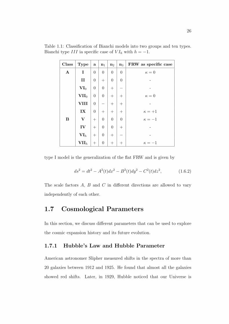
Table 1.1: Classification of Bianchi models into two groups and ten types.Bianchi type III ia specific case of V Ih with h = −1.

Class Type a n1 n2 n3 FRW as specific case

A I 0 0 0 0 κ = 0

II 0 + 0 0 -

VI0 0 0 + − -

VII0 0 0 + + κ = 0

VIII 0 − + + -

IX 0 + + + κ = +1

B V + 0 0 0 κ = −1

IV + 0 0 + -

VIh + 0 + − -

VIIh + 0 + + κ = −1

type I model is the generalization of the flat FRW and is given by

ds2 = dt2 − A2(t)dx2 −B2(t)dy2 − C2(t)dz2, (1.6.2)

The scale factors A, B and C in different directions are allowed to vary

independently of each other.

1.7 Cosmological Parameters

In this section, we discuss different parameters that can be used to explore

the cosmic expansion history and its future evolution.

1.7.1 Hubble’s Law and Hubble Parameter

American astronomer Slipher measured shifts in the spectra of more than

20 galaxies between 1912 and 1925. He found that almost all the galaxies

showed red shifts. Later, in 1929, Hubble noticed that our Universe is

27

expanding with the passage of time distant galaxies are moving away from

each other [43]. He determined the distances for a number of galaxies and

found that galaxies at larger distances also showed larger red shifts. He

constructed a linear relation between distances of galaxies from the Earth

and recessional velocity as determined by the red shifts. It can be stated

as [43] v = cz = HD, where v is the recessional velocity, H is the Hubble

constant and D is the distance from the Earth to the galaxy and z is its

redshift. This relation is called Hubble’s law. The Hubble constant or more

appropriately Hubble parameter, since it depends on time, is defined as

H =a(t)

a(t), (1.7.1)

where a(t) is the scale factor which represents cosmic expansion and dot

indicates differentiation with respect to time. a(t) is an increasing function

of time in an expanding cosmos and would be zero at the time of big-bang.

Hubble parameter represents the expansion rate that changes with time.

1.7.2 Mean and Directional Hubble Parameters

Isotropic expansion rate is specified by the Hubble parameter H as given

in Eq.(1.7.1) but in case of anisotropic expansion, we use the mean Hubble

parameter. This is the average of H in each spatial direction. If the value of

Hubble parameter varies in each spatial direction with the passage of time

then the mean Hubble parameter can be defined as

H =1

3(lnV ) = (lna) =

1

3(Hx + Hy + Hz) , (1.7.2)

where Hx, Hy and Hz represent the expansion rate with time in x, y and

z axes, respectively and known as directional Hubble parameters.

28

1.7.3 Anisotropy Parameter of Expansion

The anisotropy parameter of expansion is characterized by the mean and

directional Hubble parameters defined as

∆ =1

3

3∑i=1

(Hi −H

H

)2

, (1.7.3)

which can be represented in the form of expansion and shear scalars as

∆ = 6(σ

θ

)2

. (1.7.4)

The anisotropy of expansion results in isotropic cosmic expansion in the

limit of ∆ −→ 0.

1.7.4 Deceleration Parameter

The deceleration parameter q measures the deceleration of cosmic expansion

and is defined in terms of scale factor a(t) as well as its derivatives as

q = −a(t)a(t)

a2(t). (1.7.5)

Current observational data provided conclusive evidence for cosmic deceler-

ation that preceded the present epoch of cosmic acceleration. q can explain

the transition from past deceleration to the present accelerating epoch. The

sign of deceleration parameter indicates whether the cosmic expansion is ac-

celerating or decelerating. A positive value of q corresponds to deceleration

while the negative value indicates the accelerating behavior of cosmos. The

deceleration parameter can be expressed in the form of H as follows

q =d

dt

(1

H

)− 1 = −

(H2 + H

H2

). (1.7.6)

29

1.8 The Expansion and Shear Scalar

Let O be an open region in spacetime. A congruence in O is a family of

curves such that through each point in O there passes only one curve from

this family. Congruences generated by timelike, null and spacelike curves

are called timelike, null and spacelike congruences, respectively. Consider

the congruence of timelike geodesics (each curve in the family is a timelike

geodesic) and associated timelike vector field uα.

The expansion scalar measures the fractional rate of change of volume

per unit time and is defined as [24]

θ = uα;α = uα

,α + Γααβuβ. (1.8.1)

For θ > 0, congruence will be diverging (geodesic flying apart) which shows

that the Universe is expanding whereas for θ < 0, congruence will be con-

verging (geodesics coming closer) representing the decelerating behavior of

the Universe. The shear tensor measures the distortion in timelike curves

keeping the volume constant. It represents the possibility of initial sphere

of geodesics to become distorted into an ellipsoidal shape. It can be written

as

σαβ = θαβ − 1

3θhαβ = u(α;β) − u(αuβ) − 1

3θhαβ. (1.8.2)

The shear tensor is symmetric in its indices and shear scalar σ is given by

σ2 =1

2σαβσαβ. (1.8.3)

Chapter 2

Thermodynamics Laws inf (R, T ) and f (R, T,Q) ModifiedTheories

In this chapter, we explore the thermodynamic properties at the AH of

FRW cosmos in MGTs involving matter geometry coupling. Eling et al.

[20] suggested that non-equilibrium picture of thermodynamics is required

in non-linear MGTs such as f(R) and scalar-tensor theories. However, it has

been shown that equilibrium thermodynamics can be achieved in f(R) and

f(T ) theories by incorporating the curvature/torsion contribution terms

to the effective energy-momentum tensor [21, 23]. In our discussion, we

consider the non-equilibrium description of thermodynamics to establish

the first and second laws in f(R, T ) and f(R, T,Q) theories. We take two

forms of the energy-momentum tensor of dark components in f(R, T ) grav-

ity and demonstrate that equilibrium description of thermodynamics is not

achievable in such kind of theories. Therefore, we opt the non-equilibrium

approach and show that the field equations for these theories can be ex-

pressed in the form of FLT, ThSeff = δQ, where Seff contains contribu-

tions both from horizon entropy and an additional component introduced

due to the non-equilibrium description. The validity of GSLT is also tested

30

31

in these circumstances.

The chapter is organized in the following format. In section 2.1, we

formulate dynamical equations in f(R, T ) gravity and investigate the va-

lidity of first and second laws in this theory. Section 2.2 redefines the

contributions from exotic components in f(R, T ) gravity and explores the

thermodynamic properties in this context. Section 2.3 is devoted to the

FLT and GSLT in f(R, T,Q) and also restricts the specific forms of La-

grangian (1.1.15) for the validity of GSLT. The results presented in this

chapter have been published in [44, 45].

2.1 Thermodynamics in f (R, T ) Gravity

In this section, we first present the general formulation of dynamical equa-

tions in f(R, T ) gravity. The action of f(R, T ) gravity is given by Eq.(1.1.3)

whose variation with respect to the metric tensor yields the field equations

(1.1.6) that depend upon the source term and each choice of Lm results in

particular set of equations.

We consider the matter part as perfect fluid with Lm = −p. Conse-

quently, the field equations can be rewritten as effective Einstein equations

(1.1.11). The corresponding field equations for FRW model are

3

(H2 +

k

a2

)= 8πGeffρm +

1

fR

[1

2(RfR − f)− 3H(RfRR

+ T fRT )], (2.1.1)

−(

2H + 3H2 +k

a2

)=

1

fR

[1

2(f −RfR) + 2H(RfRR + T fRT ) + RfRR

+ R2fRRR + 2RT fRRT + T fRT + T 2fRTT

].(2.1.2)

32

These can be rewritten as

3

(H2 +

k

a2

)= 8πGeff (ρm + ρDC), (2.1.3)

−2

(H − k

a2

)= 8πGeff (ρm + ρDC + pDC), (2.1.4)

where we have assumed pressureless matter and ρDC , pDC are the energy

density and pressure of dark components

ρDC =1

8πGF[1

2(RfR − f)− 3H(RfRR + T fRT )

], (2.1.5)

pDC =1

8πGF[−1

2(RfR − f) + 2H(RfRR + T fRT ) + RfRR + R2fRRR

+ 2RT fRRT + T fRT + T 2fRTT

]. (2.1.6)

Here F = 1 + fT (R,T )8πG

. The EoS parameter of dark fluid ωDC is given by

(pDC = ωDCρDC)

ωDC = −1 + RfRR + R2fRRR + 2RT fRRT + T fRT + T 2fRTT −H(RfRR

+ T fRT )/1

2(RfR − f)− 3H(RfRR + T fRT ). (2.1.7)

The ordinary matter continuity equation involving interaction term is

of the form

ρ + 3Hρ = q. (2.1.8)

Assuming that TDCαβ behaves as perfect fluid which satisfies the following

equations

ρDC + 3H(ρDC + pDC) = qDC , (2.1.9)

ρtot + 3H(ρtot + ptot) = qtot, (2.1.10)

where ρtot = ρm+ρDC , ptot = pDC and qtot = q+qDC denote the entire energy

transfer term and qDC is the energy transfer of the fluid generated from the

33

modification to gravity. Replacing Eqs.(2.1.3) and (2.1.4) in (2.1.10), it

follows that

qtot =3

8πG(H2 +

k

a2)∂t

(fR

F)

. (2.1.11)

Clearly, this reduces to the energy transfer relation for f(R) theory if F = 1.

If the effective gravitational coupling is purely a constant, we obtain qtot = 0

implying the standard conservation law in GR.

Now, we investigate the validity of first and second laws of thermody-

namics at the AH of FRW universe.

2.1.1 First Law of Thermodynamics

The relation hαβ∂αr∂β r = 0 implies the radius of dynamical AH and for

FRW geometry it becomes

rA =

(H2 +

k

a2

)−1/2

, (2.1.12)

yielding the Hubble horizon rA = 1/H for flat case. Differentiating this

equation with respect to cosmic time, it follows that

1

Hr3A

drA

dt=

(H − k

a2

). (2.1.13)

The temperature associated with the AH is defined as [19]

Th =|κsg|2π

, (2.1.14)

where

κsg =1

2√−h

∂α(√−hhαβ∂β rA) = − 1

rA

(1−

˙rA

2HrA

)

= − rA

2

(2H2 + H +

k

a2

). (2.1.15)

34

is the surface gravity. The Bekenstein-Hawking relation Sh = A/4G [17, 18]

defines the horizon entropy in GR, while in MGTs Wald [46] suggested that

horizon entropy is associated with Noether charge and in f(R) theory it is

defined as Sh = AfR/4G. Bamba et al. [21] remarked that this entropy

relation is analogous in both metric and Palatini formalisms of f(R) gravity.

Brustein et al. [47] showed that Wald’s entropy can be represented in terms

of effective gravitational coupling as Sh = A/4Geff . Thus, one can define

the horizon entropy in f(R, T ) gravity as

Sh =AfR

4GF . (2.1.16)

This implies the corresponding results in GR and f(R) gravity depending

upon the variation of f . Employing Eqs.(2.1.13) and (2.1.16), we get

1

2πrA

dSh = 4πr3A(ρtot + ptot)Hdt +

rA

2GF dfR +rAfR

2Gd

(1

F)

. (2.1.17)

Multiplying (1− ˙rA/2HrA) on both sides of the above equation, it follows

that

ThdSh = 4πr3A(ρtot + ptot)Hdt− 2πr2

A(ρtot + ptot)drA +πr2

AThdfR

GF+

πr2AThfR

Gd

(1

F)

. (2.1.18)

In GR, the Misner-Sharp energy is defined as [48] E = rA

2Gwhich can

be extended to the form E = rA

2Geffin MGTs [49]. In terms of volume

V = 43πr3

A, we have

E =3V

8πGeff

(H2 +

k

a2

)= V ρtot, (2.1.19)

which represents the matter energy inside the sphere of radius rA. For

E > 0, one needs to set the positive effective gravitational coupling so that

35

Geff = GFfR

> 0. It follows from Eqs.(2.1.3) and (2.1.19) that

dE = −4πr3A(ρtot+ptot)Hdt+4πr2

AρtotdrA+rAdfR

2GF +rAfR

2Gd

(1

F)

. (2.1.20)

Substituting Eq.(2.1.20) in (2.1.18), we have

ThdSh = −dE + WdV +(1 + 2πrATh)rAdfR

2GF +(1 + 2πrATh)rAfR

2G

× d

(1

F)

, (2.1.21)

where W = −12T (tot)αβhαβ = 1

2(ρtot − ptot) is the work density [50]. Thus

FLT in f(R, T ) gravity can be represented as

ThdSh + ThdSh = −dE + WdV, (2.1.22)

where

dSh = − rA

2GTh

(1 + 2πrATh)d

(fR

F)

= −F(E + ShTh)

ThfR

d

(fR

F)

, (2.1.23)

is the entropy production term developed due to the non-equilibrium set-

tings in this theory as compared to GR, Gauss-Bonnet, braneworld and

Lovelock gravities [51]-[54]. dSh marks to the non-equilibrium represen-

tation of thermodynamics resulting from the effects of matter geometry

coupling. The FLT in f(R) gravity [55] and its traditional form in GR can

be recovered for f(R, T ) = f(R) and f(R, T ) = R, respectively.

2.1.2 Generalized Second Law of Thermodynamics

In literature, it has been shown that GSLT can be met in the framework

of MGTs [21, 23, 57]-[59]. It would be interesting to test the validity of

GSLT in f(R, T ) gravity. This states that the sum of entropy associated

with horizon and that of matter fluid components inside the horizon is not

36

decreasing with time. Thus one needs to show that [57]

Sh + dSh + Sin ≥ 0, (2.1.24)

where Sh is the entropy associated with AH in f(R, T ) gravity, dSh =

∂t(dSh) and Sin is the entropy of entire matter and energy sources within

horizon. The Gibb’s equation relating the entropy Sin and temperature Tin

of matter and energy sources within the horizon to the density and pressure

is given by [60]

TindSin = d(ρtotV ) + ptotdV. (2.1.25)

The temperature of matter and energy sources within the horizon is as-

sumed in proportion to the temperature of AH [56, 57, 60], i.e., Tin = bTh,

where 0 < b < 1 to ensure Tin > 0 and smaller than Th. In fact, it is natural

to assume that such proportionality relation between the temperatures of

AH and entire contents inside the horizon which results in local equilibrium

by setting the proportionality constant b as unity. In general, the horizon

temperature does not match to that of fluid components within the horizon

which makes the spontaneous flow of energy between the horizon and fluid

contents so that local thermal equilibrium is no longer preserved [60]. Fur-

thermore, mutual matter curvature coupling in these modified theories may

also play its role in energy flow and systems must experience interaction for

some period of time ahead of achieving the thermal equilibrium.

Substituting Eqs.(2.1.22) and (2.1.25) in Eq.(2.1.24), we obtain

Sh + dSh + Sin =24πΞ

rAbR≥ 0, (2.1.26)

where

Ξ = (1− b)ρtotV + (1− b

2)(ρtot + ptot)V

37

is the comprehensive constraint to meet the GSLT in MGTs [57]. Using

Eqs.(2.1.3) and (2.1.4), condition (2.1.26) becomes

12πXbRGF(H2 + k

a2 )2≥ 0, (2.1.27)

where

X = 2(1− b)H

(H − k

a2

)(H2 +

k

a2

)fR + (2− b)H

(H − k

a2

)2

fR

+ (1− b)

(H2 +

k

a2

)2

F∂t

(fR

F)

.

Therefore, the constraint to meet the GSLT is equivalent to X ≥ 0. For

flat FRW geometry, the validity of GSLT requires the conditions ∂t(fR

F ) ≥0, H > 0 and H ≥ 0. Also, F and fR are positive in order to keep E > 0.

If b = 1, i.e., temperature on either side of horizon boundary stays identical

then validity of GSLT requires

J =

(H − k

a2

)2fR

F ≥ 0. (2.1.28)

The effective EoS is given by ωeff = −1 − 2(H − ka2 )/3(H2 + k

a2 ), where

H < ka2 represents the quintessence era and H > k

a2 constitutes the phantom

regime of cosmos. Thus GSLT in f(R, T ) gravity is met in both phantom

and non-phantom eras. The validity of GSLT has also been established in

f(R) and f(T ) theories [21, 23].

2.2 Redefining the Dark Components

In the previous section, it has been found that an additional entropy term

dSh is raised in thermodynamic laws which can be regarded as the conse-

quence of non-equilibrium statement of the field equations. One can specify

the components of dark fluid so that resulting equations eliminate auxiliary

38

entropy element. Such approach is classified as an equilibrium treatment

which has been developed in MGTs [21, 23], where it is shown that one can

get rid of additional entropy production term.

We would like to explore the existence of equilibrium description in

f(R, T ) gravity. As a matter of fact, following [21, 23] we may be able to

limit the entropy production term but it cannot be eliminated completely

in this theory. We redefine the components of dark fluid so that the field

equations (2.1.3) and (2.1.4) can be rearranged with Geff =(G + fT (R,T )

8π

)

and

ρDC =1

8πGF[1

2(RfR − f)− 3H(RfRR + T fRT ) + 3(1− fR)(H2

+k

a2)

], (2.2.1)

pDC =1

8πGF[−1

2(RfR − f) + 2H(RfRR + T fRT ) + RfRR + R2fRRR

+ 2RT fRRT + T fRT + T 2fRTT − (1− fR)(2H + 3H2 +k

a2)

],(2.2.2)

being the energy density and pressure of redefined dark fluid. The EoS

parameter ωDC in this description becomes

ωDC = −1 + RfRR + R2fRRR + 2RT fRRT + T fRT + T 2fRTT −H(RfRR

+ T fRT )− 2(1− fR)(H − k

a2)/1

2(RfR − f)− 3H(RfRR + T fRT )

+ 3(1− fR)(H2 +k

a2). (2.2.3)

It is evident from Eqs.(2.1.7) and (2.2.3) that the EoS parameter is not

unique in both cases. Thus one should regard the two formulations of dark

fluid in discussions on cosmic issues.

The entire energy exchange term for this case turns out to be

qtot =3

8πG(H2 +

k

a2)∂t

(1

F)

. (2.2.4)

39

Since in general ∂t(fT (R, T )) 6= 0 in this theory, so qtot is non-zero. However,

it may disappear in some specific cases which involve the linear dependence

on T such as f(R, T ) = f(R)+cT and results would be very similar to that

in f(R) gravity. Therefore, we may not be able to develop the equilibrium

picture of thermodynamics in f(R, T ) gravity. Consequently, we again need

to consider the non-equilibrium treatment of thermodynamics. This result

differentiates f(R, T ) gravity from other MGTs due to the matter depen-

dence of the Lagrangian density. In f(R) and f(T ) theories, the redefinition

of dark fluid results in local conservation of the energy-momentum tensor

of dark components [21, 23].

Now we explore the validity of the first and second laws of thermody-

namics in this setting.

2.2.1 First Law of Thermodynamics

In this particular representation of dark fluid, the time derivative of radius

rA at the AH is given by

drA = 4πr3AGF(ρtot + ptot)Hdt. (2.2.5)

In f(R, T ) gravity, the equilibrium description is not executable as com-

pared to other MGTs such as f(R), f(T ) and scalar-tensor theories etc.

Thus, we employ the Wald entropy relation Sh = A/(4Geff ) rather than

introducing Bekenstein-Hawking entropy. For this case, the differential of

horizon entropy is given by

1

2πrA

dSh = 4πr3A(ρtot + ptot)Hdt +

rA

2Gd

(1

F)

. (2.2.6)

40

The evolution of entropy can be represented in terms of temperature as

ThdSh = 4πr3A(ρtot + ptot)Hdt− 2πr2

A(ρtot + ptot)drA +πr2

ATh

G

×(

1

F)

. (2.2.7)

Introducing the Misner-Sharp energy

E =rA

2GF = V ρtot, (2.2.8)

we obtain

dE = −4πr3A(ρtot + ptot)Hdt + 4πr2

AρtotdrA +rA

2Gd

(1

F)

. (2.2.9)

Combining Eqs.(2.2.7) and (2.2.9), it gives the FLT

ThdSh + ThdSh = −dE + WdV, (2.2.10)

where

dSh = − rA

2ThG(1 + 2πrATh)d

(1

F)

= −F(

E

Th

+ Sh

)d

(1

F)

= − π(4H2 + H + 3k/a2)

G(H2 + k/a2)(2H2 + H + k/a2)d

(1

F)

, (2.2.11)

is an additional entropy term produced due to matter contents of the cos-

mos. It involves derivative of f(R, T ) with respect to T . Notice that the

FLT, ThdSh = −dE + WdV holds at the AH of FRW universe in equilib-

rium description of MGTs [21, 23, 56]. However, in f(R, T ) gravity, this

law does not hold due to the presence of an additional term dSh. This

term vanishes if we take f(R, T ) = f(R) which leads to the equilibrium

description of thermodynamics in f(R) gravity.

41

2.2.2 Generalized Second Law of Thermodynamics

To formulate the GSLT in this description of f(R, T ) gravity, we consider

the Gibbs equation in terms of all matter fields and energy contents

TindSin = d(ρtotV ) + pindV, (2.2.12)

where Tin and Sin denote the temperature and entropy of all the matter

and energy sources within the horizon. For this representation, the GSLT

can be represented as

˙Sh + d

˙Sh +

˙Stot ≥ 0, (2.2.13)

which implies that

12πYbRGF(H2 + k

a2 )2≥ 0, (2.2.14)

where

Y = 2(1− b)H

(H − k

a2

)(H2 +

k

a2

)+ (2− b)H

(H − k

a2

)2

+ (1− b)

(H2 +

k

a2

)2

F∂t

(1

F)

.

Thus the GSLT is met only if Y ≥ 0. For flat FRW geometry, the GSLT

is satisfied with the constraints ∂t(1F ) ≥ 0, H > 0 and H ≥ 0. In thermal

equilibrium b = 1, the above constraint is reduced to

B =12πH

(H − k

a2

)2

G(H2 + k

a2

)2R

1

F ≥ 0, (2.2.15)

for V = 43πr3

A and R = 6(H + 2H2 + k/a2). B ≥ 0 clearly holds when

the Hubble parameter and scalar curvature have the same signatures. It

can be seen that significant conflict of results of f(R, T ) with f(R) gravity

is the factor F = 1 + fT (R,T )8πG

. We remark that in both definitions of dark

components, the GSLT is met both in phantom and non-phantom cosmic

eras.

42

2.3 Thermodynamics in f (R, T,Q) Gravity

In this section, we consider more general modified gravity involving the

dependence on matter energy-momentum tensor whose action is presented

in Eq.(1.1.15). The variation of action (1.1.15) with respect to metric im-

plies field equations in f(R, T,Q) gravity which are shown in Eqs.(1.1.16)-

(1.1.18). For perfect fluid as the matter energy-momentum tensor the (0−0)

and (i− i) components of TDCαβ can be determined as

T(DC)00 =

1

fR − fQLm

[1

2(f −RfR)− LmfT − 3H∂tfR +

3

2

(H2 + 3H

)

× ρfQ − 3

2

(3H2 + H

)pfQ +

3

2H∂t [(p− ρ)fQ] +

3

2Hρ∂tfQ

+1

2ρ∂ttfQ

], (2.3.1)

T(DC)ii =

1

fR − fQLm

[1

2(RfR − f) + LmfT +

1

2

(H + 3H2

)ρfQ

+1

2

(5(3H2 + H) +

8κ

a2

)pfQ + 2H∂t fR + (ρ + p) fQ

+ ∂tt

fR +

1

2(ρ− p)fQ

+

3

2Hp∂tfQ +

1

2p∂ttfQ

]gii, (2.3.2)

where ρ, p represent the energy density and pressure of matter fluid. Using

Eqs.(2.3.1) and (2.3.2), the field equations in f(R, T,Q) gravity can be

rearranged as

−2

(H − k

a2

)= 8πGeff (ρ + p) +

1

fR − fQLm

[(3H2 + 5H)ρfQ

+ (3H2 + H +4κ

a2)pfQ −H∂tfR − 1

2(ρ + 7p)fQ

+3

2H(ρ + p)∂tfQ + ∂ttfR +

1

2(ρ− p)fQ+

1

2(ρ + p)

× ∂ttfQ] . (2.3.3)

The covariant divergence of the energy-momentum tensor can be set by

43

taking the divergence of the field equation (1.1.16), yielding

∇µTµν =2

2(1 + fT ) + RfQ

[∇µ(fQRαµTαν) +∇ν(LmfT )− 1

2(fQRσζ

+ fT gσζ)∇νTσζ −Gµν∇µ(fQLm)− 1

2[∇µ(RfQ) + 2∇µfT ] Tµν

].

(2.3.4)

For FRW spacetime, the matter energy density ρ satisfies

ρ + 3H(ρ + p) =1

2 + 3(fT − (H + 3H2)fQ)

[3

H(H − 3H2)(ρ + p)

− (H + 2H2)∂tp− 2H2∂tLm

fQ + 6H2(ρ− Lm)∂tfQ + fT ∂t(2Lm + 3p)

+ 2(Lm − ρ)∂tfT ] . (2.3.5)

It is significant to see that ideal continuity equation does not agree in this

modified theory which is also true in other modified theories involving non-

minimal matter geometry coupling [12, 13, 14]. This equation represents

the standard continuity equation when the left side vanishes which is only

possible if Lagrangian has null variation with respect to T and Q.

Now, we analyze thermodynamic properties in f(R, T,Q) gravity and

discuss the first and second laws of thermodynamics at the AH of FRW

universe. In section 2.2, it is shown that equilibrium description may not

be achievable in f(R, T ) gravity. As this theory is more general to f(R, T )

gravity, therefore we adopt the non-equilibrium description of thermody-

namics.

44

2.3.1 First Law of Thermodynamics

Let us proceed to establish FLT in the above modified theory. Substituting

Eq.(2.3.3) in (2.1.13) and multiplying with the factor 4πrA, we obtain

1

2πrA

16π2rA(fR − fQLm)drA

κ2 + fT + 12(R−2)fQ

=4πr3

AH

κ2 + fT + 12(R−2)fQ

[(3H2 + 5H)

× ρfQ + (3H2 + H +4κ

a2)pfQ −H∂tfR − 1

2(ρ + 7p)fQ+

3

2H(ρ + p)

× ∂tfQ + ∂ttfR +1

2(ρ− p)fQ+

1

2(ρ + p)∂ttfQ

]dt + 4πr3

AH(ρ + p)dt.

(2.3.6)

We define the following differential

d

(8πA(fR − fQLm)

4(κ2 + fT + 12(R−2)fQ)

)=

8πrA

κ2 + fT + 12(R−2)fQ)

[2π(fR

− fQLm)drA + rA

∂t(fR − fQLm)− (fR − fQLm)∂t

(ln[κ2 + fT

− 1

2(R−2)fQ]

)dt

],

so that Eq.(2.3.6) is modified to the form

1

2πrA

d

(8πA(fR − fQLm)

4(κ2 + fT + 12(R−2)fQ)

)= 4πr3

AH[(ρ + p) +

(3H2

+ 5H)ρfQ + (3H2 + H +4κ

a2)pfQ −H∂tfR − 1

2(ρ + 7p)fQ+

1

2(ρ + p)

× (3H∂tfQ + ∂ttfQ) + ∂ttfR +1

2(ρ− p)fQ

/

(κ2 + fT +

1

2(R−2)

× fQ)] dt +rA

2

8π

κ2 + fT + 12(R−2)fQ

∂t(fR − fQLm)− (fR − fQLm)

× ∂t

(ln[κ2 + fT − 1

2(R−2)fQ]

)dt. (2.3.7)

Moreover, if we multiply the above equation by the term (1− ˙rA/2HrA),

45

one can obtain

|κsg|2π

d

(8πA(fR − fQLm)

4(κ2 + fT + 12(R−2)fQ)

)=

(1−

˙rA

2HrA

)4πr3

AH [(ρ + p)

+

(3H2 + 5H)ρfQ + (3H2 + H +

4κ

a2)pfQ −H∂tfR − 1

2(ρ + 7p)fQ

+1

2(ρ + p)(3H∂tfQ + ∂ttfQ) + ∂ttfR +

1

2(ρ− p)fQ

/

(κ2 + fT +

1

2

× (R−2)fQ)] dt +

(1−

˙rA

2HrA

)rA

2

8π

κ2 + fT + 12(R−2)fQ

∂t(fR

− fQLm)− (fR − fQLm)∂t

(ln[κ2 + fT − 1

2(R−2)fQ]

)dt, (2.3.8)

where κsg = 1rA

(1 − ˙rA

2HrA) is the surface gravity and |κsg|

2πis identified as

temperature of AH. The term inside the differential on left side of the

above equation is the entropy [55, 61], S = 8πA(fR−fQLm)

4(κ2+fT + 12(R−2)fQ)

|rAof AH

in f(R, T,Q) gravity. The entropy relation in f(R, T,Q) gravity repro-

duces the corresponding results in f(R) [55, 21] and f(R, T ) [44] theories.

Consequently, Eq.(2.3.8) can be rewritten as

ThdS = 4πr3AH(ρ + p)dt− 2πr2

A(ρ + p)drA +2πAHr2

A

κ2 + fT + 12(R−2)fQ

× T

(3H2 + 5H)ρfQ + (3H2 + H +

4κ

a2)pfQ −H∂tfR − 1

2(ρ

+ 7p)fQ+1

2(ρ + p)(3H∂tfQ + ∂ttfQ) + ∂ttfR +

1

2(ρ− p)fQ

dt

+TA

4

8π

κ2 + fT + 12(R−2)fQ

∂t(fR − fQLm)− (fR − fQLm)

× ∂t

(ln[κ2 + fT − 1

2(R−2)fQ]

)dt. (2.3.9)

Taking differential of energy relation E = V ρ, we get

dE = 4πr2AρdrA +

4

3πr3

Aρdt. (2.3.10)

Using the expression of time derivative of energy density (2.3.5), the

46

above result takes the following form

dE = 4πr2AρdrA − 4πr3

A(ρ + p)Hdt +V

2 + 3(fT − (H + 3H2)fQ))[3 H

× (H − 3H2)(ρ + p)− (H + 2H2)∂tp− 2H2∂tLm

fQ + 6H2(ρ− Lm)

× ∂tfQ + fT ∂t(2Lm + 3p) + 2(Lm − ρ)∂tfT ] dt. (2.3.11)

Incorporating dE in Eq.(2.3.9), it follows that

ThdSh = −dE +1

2(ρ− p)d(4/3πr3

A) +TA

4[G + (fT + 12(R−2)fQ)/8π]

×[Hr2

A

(3H2 + 5H)ρ + (3H2 + H +

4κ

a2)p

fQ + (1−H2r2

A)∂tfR +1

2

× H2r2A∂t[(ρ + p)fQ] +

3

2H2r2

A(ρ + p)∂tfQ − ∂t(fQLm) + Hr2A ∂tt (fR

+1

2(ρ− p)fQ

)+

1

2(ρ + p)∂ttfQ

− (fR − fQLm)∂t(ln[κ2 + fT +

1

2(R

+ 2)fQ])] dt +2πV

|κ|[2 + 3(fT − (H + 3H2)fQ)]

3

H(H − 3H3)(ρ + p)

− (H + 2H2)∂tp− 2H2∂tLm

fQ + fT ∂t(2Lm + 3p) + 2(ρ− Lm)(3H2

× ∂tfQ − ∂tfT ) dt. (2.3.12)

As the work density is defined as W = 12(ρ − p), so the above equation

implies FLT in this modified theory as follows

ThdSh + ThdSh = −dE + WdV, (2.3.13)

where

dSh =−TA

4[G + (fT + 12(R−2)fQ)/8π]

[Hr2

A

(3H2 + 5H)ρ + (3H2

+ H +4κ

a2)p

fQ + (1−H2r2

A)∂tfR +1

2H2r2

A∂t[(ρ + 7p)fQ] +3

2H2r2

A(ρ

+ p)∂tfQ − ∂t(fQLm) + H2r2A

∂tt

(fR +

1

2(ρ− p)fQ

)+

1

2(ρ + p)∂ttfQ

− (fR − fQLm)∂t(ln[κ2 + fT +1

2(R + 2)fQ])

]dt+

47

2πV

3

H(H − 3H2)(ρ + p)− (H + 2H2)∂tp− 2H2∂tLm

fQ

+ fT ∂t(2Lm + 3p) + 2(ρ− Lm)(3H2∂tfQ − ∂tfT )

dt/|κ|[2 + 3(fT

− (H + 3H2)fQ)],

is the entropy production term developed in this modified theory. Such

additional term marks to the non-equilibrium treatment of thermodynamics

and is produced internally due to matter curvature coupling.

In gravitational theories such as Einstein, Gauss-Bonnet, braneworld

and Lovelock gravities, the usual FLT is satisfied by the respective field

equations. In fact, these theories do not involve any surplus term in univer-

sal form of FLT, i.e., TdS = −dE +WdV . It is worth mentioning here that

FLT for non-equilibrium treatment in f(R, T ) gravity can be retrieved from

this result if Lagrangian (1.1.15) has null variation with respect to Q so that

f(R, T,Q) = f(R, T ). One can also obtain FLT exclusively in f(R) theory

by setting f(R, T,Q) = f(R) which is similar to that in [55] for (3+1)-

dimensional FRW spacetime while it does correspond to GR if fT = fQ = 0

and fR = 1 so that dSh vanishes. Thus FLT (2.3.13) established in this

modified theory is more comprehensive and ensures the results in f(R) and

f(R, T ) theories. One can define the effective entropy term being the sum

of horizon entropy and entropy production term as Seff = Sh + S so that

Eq.(2.3.13) can be rewritten as

ThdSeff = −dE + WdV,

where Seff is the effective entropy related to the CMC in this modified

theory at the AH of FRW spacetime.

48

2.3.2 Generalized Second Law of Thermodynamics

Here, we explore the validity of GSLT in the framework of f(R, T,Q) grav-

ity. Let us proceed with the Gibb’s equation which relates the entropy of

matter and energy sources to the pressure in the horizon given by

TindSin = (ρ + p)dV + V dρ. (2.3.14)

Using the divergence of energy-momentum tensor, we can evaluate the evo-

lution of entropy inside the horizon as

TinSin = 4πr2A(ρ + p)( ˙rA −HrA) +

V

2 + 3(fT − (H + 3H2)fQ)3 H

× (H − 3H3)(ρ + p)− (H + 2H2)∂tp− 2H2∂tLm

fQ + fT ∂t(2Lm

+ 3p) + 2(ρ− Lm)(3H2∂tfQ − ∂tfT )

. (2.3.15)

One can find the relations of matter energy density and pressure for the

FRW universe using the field equation (1.1.16) as follows

ρ =1

κ2 + fT + 12(R−2)fQ

[1

2f − 3(H + H2)fR + Lm(fT − 3(H2 +

κ

a2)

× fQ)− 3

2

(H2 + 3H

)ρfQ +

3

2

(3H2 + H

)pfQ + 3H∂t

(fR +

1

2[(ρ

− p)fQ])− 3

2Hρ∂tfQ − 1

2ρ∂ttfQ

], (2.3.16)

p =1

κ2 + fT + 12(R−2)fQ

[1

2f + Lm

((2H + 3H2 +

κ

a2)− fT

)+ (H

+ 3H2 +2κ

a2)fR − 1

2

(H + 3H2

)ρfQ − 1

2

(5(3H2 + H) +

8κ

a2

)pfQ

− 2H∂t fR + (ρ + p) fQ − ∂tt

fR +

1

2(ρ− p)fQ

− 3

2Hp∂tfQ

− 1

2p∂ttfQ

]. (2.3.17)

49

Substituting Eqs.(2.3.16) and (2.3.17) in (2.3.15), it follows that

TinSin = 4πr2A( ˙rA −HrA)

1

κ2 + fT + 12(R−2)fQ

[2(

κ

a2− H)(fR

− fQLm)− (3H2 + 5H)ρfQ − (3H2 + H +4κ

a2)pfQ + H∂tfR

− 1

2(ρ + 7p)fQ − 1

2(ρ + p)(3H∂tfQ + ∂ttfQ)− ∂ttfR +

1

2(ρ

− p)fQ] V

2 + 3(fT − (H + 3H2)fQ)

3

H(H − 3H3)(ρ + p)

− (H + 2H2)∂tp− 2H2∂tLm

fQ + fT ∂t(2Lm + 3p)

+ 2(ρ− Lm)(3H2∂tfQ − ∂tfT )

. (2.3.18)

The entropy of AH in f(R, T,Q) gravity is defined as

Sh =A(fR − fQLm)

4[G + 18π

(fT + 12(R−2)fQ)]

. (2.3.19)

The evolution of Sh multiplied with the horizon temperature implies that

ThSh =2π(2HrA − ˙rA)

κ2 + fT + 12(R−2)fQ

[2

˙rA

rA

(fR − fQLm) + ∂t(fR − fQLm)−

× (fR − fQLm)∂tκ2 + fT +1

2(R−2)fQ

]. (2.3.20)

Eventually, the validity of GSLT requires the condition (ThSh+ TinSin) > 0.

In this setting, we assume a relation between Tin and Th as Tin = bTh.

After some manipulations, Eqs.(2.3.18) and (2.3.20) can be summed to the

following form

ThStot =2π

(H2 + κ

a2

)−5/2

κ2 + fT + 12(R−2)fQ

[2H

( κ

a2− H

) κ

a2+ (1− 2b)H + 2(1

− b)H2

(fR − fQLm) + ∂tfR

κ

a2

( κ

a2+ H + 3H2

)+ (1− 2b)H

× H2 + 2(1− b)H4

+ 2bH(H + H2)∂ttfR − (κ

a2+ H2)

( κ

a2+ H

+ 2H2)

(fR − fQLm)∂t

[ln

(κ2 + fT +

1

2(R−2)fQ

)]+ ∂t(fQ

× Lm)]

50

−4bπ(H2 + κ

a2

)−5/2H(H + H2)

κ2 + fT + 12(R−2)fQ

[−(3H2 + 5H)ρfQ − (3H2 + H

+4κ

a2)pfQ − 1

2H∂t(ρ + 7p)fQ − 1

2(ρ + p)(3H∂tfQ + ∂ttfQ)− ∂ttfR

+1

2(ρ− p)fQ

]+

43bπr3

A

2 + 3[fT − (H + 3H2)fQ]

3

H(H − 3H2)(ρ

+ p)− (H + 2H2)∂tp− 2H2∂tLm

fQ + fT ∂t(2Lm + 3p) + 2(ρ

− Lm)(3H2∂tfQ − ∂tfT )

> 0, (2.3.21)

where Stot = Sh +Sin and condition to meet the GSLT counts the choice of

action in this modified theory. The above result appears to be more general

and one can deduce the expressions of GSLT in Einstein, f(R) and f(R, T )

gravities.

If we set f(R, T,Q) = f(R, T ), so that the variation of f with respect

to Q is null then inequality to fulfill the GSLT is given by

ThStot =2π

(H2 + κ

a2

)−5/2

κ2 + fT

[2H

( κ

a2− H

) κ

a2+ (1− 2b)H + 2(1− b)

× H2

fR + ∂tfR

κ

a2

( κ

a2+ H + 3H2

)+ (1− 2b)HH2 + 2(1− b)H4

+ 2bH(H + H2)∂ttfR −( κ

a2+ H2

)( κ

a2+ H + 2H2

)fR∂t[ln(κ2 + fT )]

+4

3πr3

A

b

2 + 3fT

fT ∂t(2Lm + 3p) + 2(Lm − ρ)∂tfT]

> 0. (2.3.22)

When fT = fQ = 0 (purely f(R) gravity), the GSLT takes the form

ThStot =2π

(H2 + κ

a2

)−5/2

κ2

[2H

( κ

a2− H

) κ

a2+ (1− 2b)H + 2(1− b)

× H2

fR + κ

a2

( κ

a2+ H + 3H2

)+ (1− 2b)HH2 + 2(1− b)H4

∂tfR

+ 2bH(H + H2)∂ttfR

]> 0. (2.3.23)

The GSLT in Einstein gravity can be recovered by replacing fR = 1 in

Eq.(2.3.23)

ThStot =1

2GH

(H − κ

a2

)2 (H2 +

κ

a2

)−5/2

.

51

We limit our discussion of GSLT by taking the system (includes matter

and energy contents bounded by the horizon) in equilibrium position so

that energy would not flow in the system and temperature within the hori-

zon more or less matches with the horizon temperature, i.e., b = 1. This

situation would correspond to the case of late times where the universe

components and horizon would have interacted for long time while its ex-

istence for early or intermediate times would be ambiguous. Though the

assumption of thermal equilibrium is limiting in some sense to avoid the

non-equilibrium complexities but it has widely been accepted to study the

GSLT [21, 23, 57, 58, 59, 61].

To illustrate the validity of GSLT in f(R, T,Q) gravity, we take some

concrete models in this modified theory namely [13]

(i) f(R, T,Q) = R + αQ, (ii) f(R, T,Q) = R(1 + αQ),

where α is a coupling parameter. These models are proposed in [13] where

authors explored the evolution of scale factor and deceleration parameter in

this scenario. Recently, we have examined the validity of energy conditions

for the above particular forms of Lagrangian (1.1.15) [62]. Here we are

interested to develop constraints on the validity of GSLT.

(i) f(R, T,Q) = R + αQ

For this model, the GSLT becomes

ThStot =2π

(H2 + κ

a2

)−5/2

κ2 + α2R

[2H

( κ

a2− H

)2

(1− αLm)−( κ

a2+ H2

)( κ

a2

+ H + 2H2)

(1− αLm)∂t

[ln

(κ2 +

α

2R

)]+ α∂tLm

− 2H(H

+ H2)

−(3H2 + 5H)αρ− (3H2 + H +

4κ

a2)αp− α

2H(ρ + 7p)

− α

2(ρ− p)

]

52

+4πα

(κa2 + H2

)−3/2

2− 3α(H + 3H2)

H(H − 3H2)(ρ + p)− (H + 2H2)∂tp

− 2H2∂tLm

> 0.

Cosmic expansion history is thought to have experienced the decelerated

phase and hence transition to accelerating epoch. Thus, power law solutions

can play vital role to connect the matter dominated phase with accelerating

paradigm. The existence of power law solutions in FRW setting is partic-

ularly relevant to intimate all possible cosmic evolutions. The scale factor

for power law cosmology is defined as

a(t) = a0tm,

where m is a positive constant. If 0 < m < 1, then the resulting power

law solution favors decelerating expansion whereas for m > 1, it exhibits

accelerating behavior. To be more explicit for the above constraint, we set

the power law cosmology for accelerated cosmic expansion (m > 1) with

ρ = ρ0t−3m and choose Lm = −p. For the flat FRW geometry, the plots of

GSLT are shown in Figure 2.1. We find that the GSLT holds if one sets

the parameters as α < 0 and m > 1 while in the case of Lm = ρ, it can be

easily examined that validity of GSLT requires m > 8.

(ii) f(R, T,Q) = R(1 + αQ)

In this case, Eq.(2.3.21) takes the form

ThStot =2π

(H2 + κ

a2

)−5/2

κ2 + α2(R−2)R

[2H

( κ

a2− H

)2

(1−RαLm)−( κ

a2+ H2

)

×( κ

a2+ H + 2H2

)(1−RαLm)∂t

[ln

(κ2 +

α

2(R−2)R

)]+ α

× ∂t(RLm) − 2H(H + H2)−αρ(3H2 + 5H)R− αp(3H2 + H

+4κ

a2)R− α

2H∂[(ρ + 7p)R]− 3α

2H(ρ + p)R− α

2∂tt[(ρ− p)R]

]

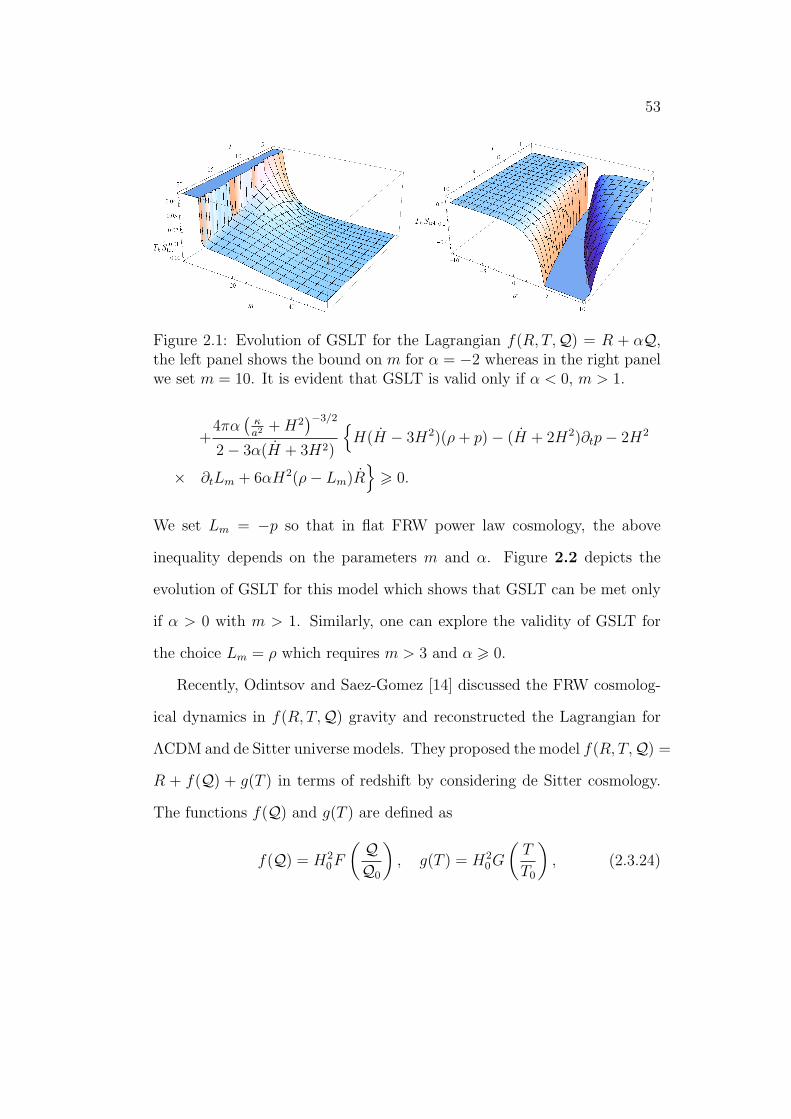
53

Figure 2.1: Evolution of GSLT for the Lagrangian f(R, T,Q) = R + αQ,the left panel shows the bound on m for α = −2 whereas in the right panelwe set m = 10. It is evident that GSLT is valid only if α < 0, m > 1.

+4πα

(κa2 + H2

)−3/2

2− 3α(H + 3H2)

H(H − 3H2)(ρ + p)− (H + 2H2)∂tp− 2H2

× ∂tLm + 6αH2(ρ− Lm)R

> 0.

We set Lm = −p so that in flat FRW power law cosmology, the above

inequality depends on the parameters m and α. Figure 2.2 depicts the

evolution of GSLT for this model which shows that GSLT can be met only

if α > 0 with m > 1. Similarly, one can explore the validity of GSLT for

the choice Lm = ρ which requires m > 3 and α > 0.

Recently, Odintsov and Saez-Gomez [14] discussed the FRW cosmolog-

ical dynamics in f(R, T,Q) gravity and reconstructed the Lagrangian for

ΛCDM and de Sitter universe models. They proposed the model f(R, T,Q) =

R + f(Q) + g(T ) in terms of redshift by considering de Sitter cosmology.

The functions f(Q) and g(T ) are defined as

f(Q) = H20F

( QQ0

), g(T ) = H2

0G

(T

T0

), (2.3.24)

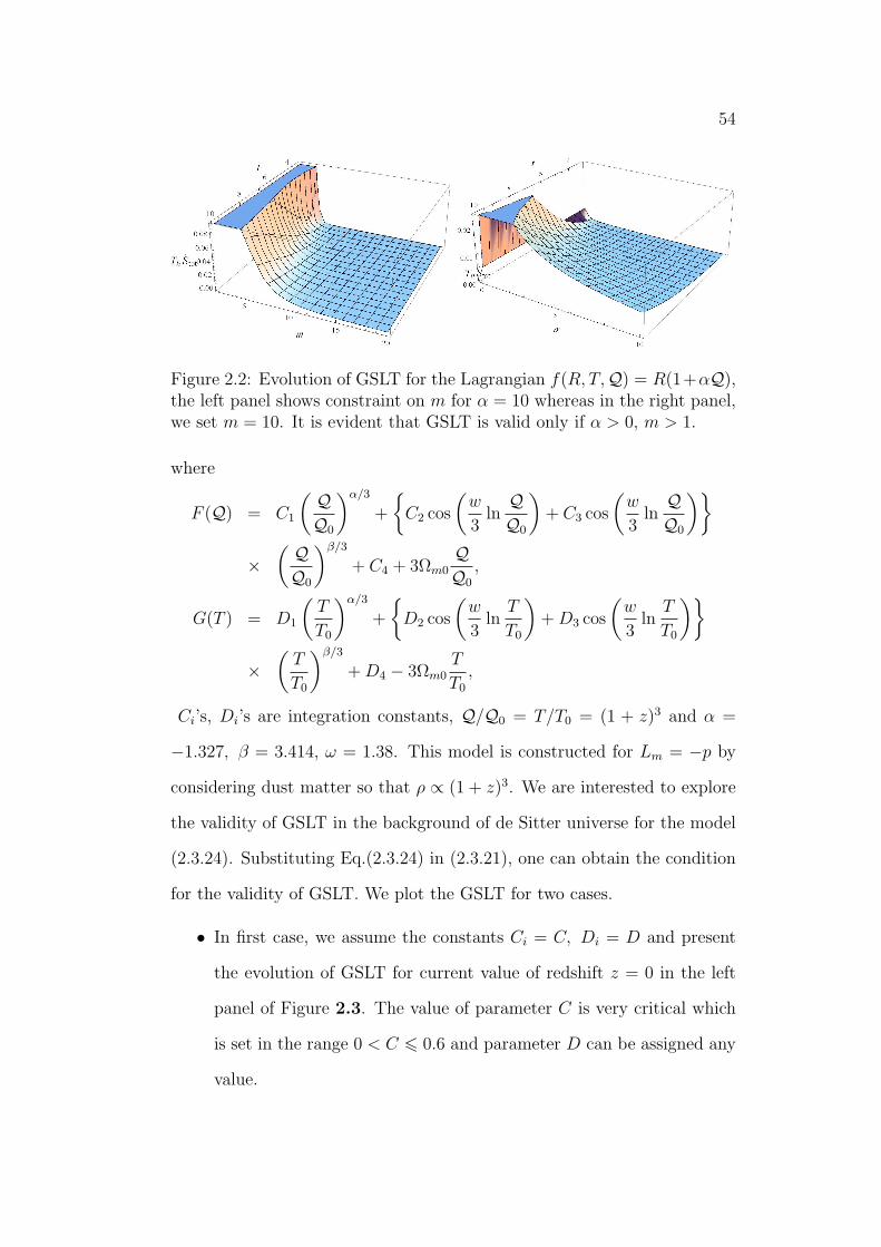
54

Figure 2.2: Evolution of GSLT for the Lagrangian f(R, T,Q) = R(1+αQ),the left panel shows constraint on m for α = 10 whereas in the right panel,we set m = 10. It is evident that GSLT is valid only if α > 0, m > 1.

where

F (Q) = C1

( QQ0

)α/3

+

C2 cos

(w

3lnQQ0

)+ C3 cos

(w

3lnQQ0

)

×( QQ0

)β/3

+ C4 + 3Ωm0QQ0

,

G(T ) = D1

(T

T0

)α/3

+

D2 cos

(w

3ln

T

T0

)+ D3 cos

(w

3ln

T

T0

)

×(

T

T0

)β/3

+ D4 − 3Ωm0T

T0

,

Ci’s, Di’s are integration constants, Q/Q0 = T/T0 = (1 + z)3 and α =

−1.327, β = 3.414, ω = 1.38. This model is constructed for Lm = −p by

considering dust matter so that ρ ∝ (1 + z)3. We are interested to explore

the validity of GSLT in the background of de Sitter universe for the model

(2.3.24). Substituting Eq.(2.3.24) in (2.3.21), one can obtain the condition

for the validity of GSLT. We plot the GSLT for two cases.

• In first case, we assume the constants Ci = C, Di = D and present

the evolution of GSLT for current value of redshift z = 0 in the left

panel of Figure 2.3. The value of parameter C is very critical which

is set in the range 0 < C 6 0.6 and parameter D can be assigned any

value.

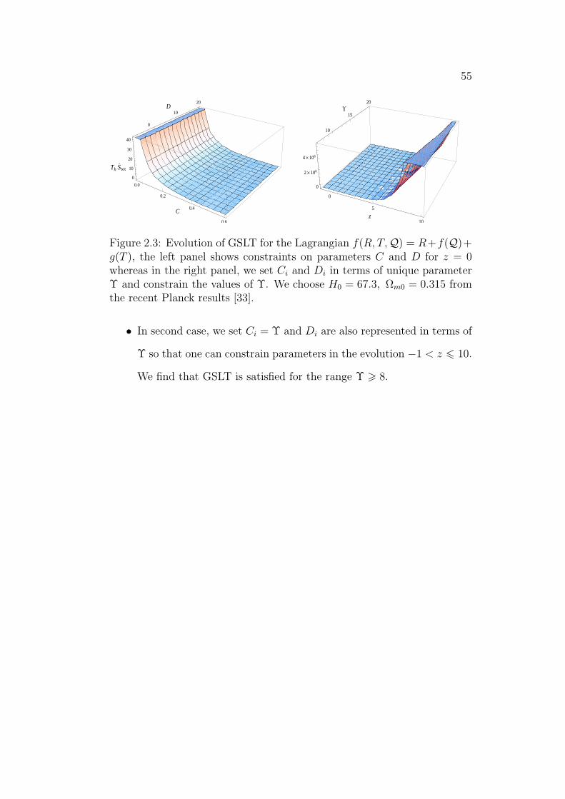
55

0.0

0.2

0.4

0.6

C

0

10

20D

0

10

20

30

40

Th S

tot

0

5

10z

10

15

20U

0

2´106

4´106

Figure 2.3: Evolution of GSLT for the Lagrangian f(R, T,Q) = R+f(Q)+g(T ), the left panel shows constraints on parameters C and D for z = 0whereas in the right panel, we set Ci and Di in terms of unique parameterΥ and constrain the values of Υ. We choose H0 = 67.3, Ωm0 = 0.315 fromthe recent Planck results [33].

• In second case, we set Ci = Υ and Di are also represented in terms of

Υ so that one can constrain parameters in the evolution −1 < z 6 10.

We find that GSLT is satisfied for the range Υ > 8.

Chapter 3

Energy Conditions Constraintsand Stability of f (R, T ) andf (R, T,Q) Modified Theories

In this chapter, we present the energy conditions constraints in the context

of f(R, T ) and f(R, T,Q) theories. The corresponding energy conditions

appear to be more general and can reduce to the familiar forms of these

conditions in GR and f(R) theory. The generic inequalities set by these

energy constraints are presented in terms of recent values of Hubble, de-

celeration, jerk and snap parameters. In particular, some specific models

are considered in these theories to study the concrete application of energy

bounds as well as the Dolgov-Kawasaki instability. Moreover, we obtain

the exact power law solutions for two particular cases namely, f(R) + λT

and R + 2f(T ) in homogeneous and isotropic f(R, T ) cosmology. We also

establish certain conditions to ensure the viability of these solutions.

The present chapter has the following format. In section 3.1, we derive

the energy conditions in f(R, T,Q) gravity and respective inequalities are

presented in terms of cosmographic parameters. Section 3.2 is devoted to

study the energy conditions bounds for some specific forms of f(R, T,Q)

gravity and the Dolgov-Kawasaki instability. In section 3.3, the energy

56

57

constraints are also shown for specific functional forms of f(R, T ) involv-

ing an exponential function and the coupling between R and T . We also

explore the existence of power law solutions and corresponding constraints

from energy conditions. Section 3.4 is devoted to examine whether these

solutions are stable against linear homogeneous perturbations in f(R, T )

gravity. This chapter is based upon the results presented in [62, 63].

3.1 Energy Conditions in f (R, T,Q) Gravity

In this section, we derive the energy conditions in the context of f(R, T,Q)

gravity and express in terms of well-known cosmographic parameters. The

field equation (1.1.16) can be rearranged in the following form

Gαβ = Rαβ − 1

2Rgαβ = T eff

αβ , (3.1.1)

which is analogous to the standard field equations in GR. Here T effαβ , the

effective energy-momentum tensor in f(R, T,Q) gravity is defined as

T effαβ =

1

fR − fQLm

[(1 + fT +

1

2RfQ)Tαβ + 1

2(f −RfR)− LmfT

− 1

2∇α∇β(fQTαβ)gαβ − (gαβ2−∇α∇β)fR − 1

22(fQTαβ)

− 2fQRα(αTαβ) +∇α∇(α[T α

β)fQ] + 2(fT gαβ + fQRαβ

)

× ∂2Lm

∂gαβ∂gαβ

]. (3.1.2)

We take the homogeneous and isotropic flat FRW metric defined as

ds2 = dt2 − a2(t)dx2,

where dx2 is the spatial part of the metric. The corresponding effective

energy density and effective pressure can be taken such that T effαβ assumes

58

the form of perfect fluid. In FRW background, ρeff and peff can be obtained

in this modified theory as

ρeff =1

fR − fQLm

[ρ + (ρ− Lm)fT +

1

2(f −RfR)− 3H∂tfR − 3

2(3H2

− H)ρfQ − 3

2(3H2 + H)pfQ +

3

2H∂t[(p− ρ)fQ]

], (3.1.3)

peff =1

fR − fQLm

[p + (p + Lm)fT +

1

2(RfR − f) +

1

2(H + 3H2)(ρ

− p)fQ + ∂ttfR + 2H∂tfR +1

2∂tt[(ρ− p)fQ] + 2H∂t[(ρ + p)

× fQ]] , (3.1.4)

where R = −6(H + 2H2), H = aa

being Hubble parameter and over dot

refers to time derivative. Here, we neglect the terms involving second deriv-

ative of matter Lagrangian with respect to the metric tensor. As we are

dealing with perfect fluid, so matter Lagrangian can either be Lm = p or

Lm = −ρ which makes it obvious to ignore such term.

We adopt the procedure developed in [28, 32] for f(R), f(R,Lm) and

f(R) gravity with arbitrary and non-minimal matter geometry coupling

to extend it to a more general f(R, T,Q) grvaity. The Ricci tensor in

Eq.(3.1.1) can be represented in terms of T effαβ and its trace T eff as

Rαβ = T effαβ − 1

2gαβT eff , (3.1.5)

where the contraction of Eq.(3.1.2) yields the trace of the energy-momentum

tensor

T eff =1

fR − fQLm

[(1 + fT +

1

2RfQ)T + 2(f −RfR)− 4LmfT

− ∇α∇β(fQTαβ)− 32fR − 1

22(fQT )− 2fQRαβTαβ + 2gαβ(fT gαβ

+ fQRαβ)∂2Lm

∂gαβ∂gαβ

]. (3.1.6)

59

The attractive nature of gravity needs to satisfy the following additional

constraint

1 + fT + 12RfQ

fR − fQLm

> 0, (3.1.7)

which does not depend on the conditions (1.5.3) derived from the Ray-

chaudhuri equation. In fact, this condition corresponds to the effective

gravitational coupling in f(R, T,Q) gravity.

In section 1.5, it is shown that Raychaudhuri equations with attractive

behavior of gravitational interaction give rise to SEC and NEC which hold

for any theory of gravitation. In this modified theory, we can employ an

approach analogous to that in GR to develop the energy conditions. We

also assume that standard matter obeys the energy conditions. We combine

Eqs.(1.5.4) and (3.1.6) so that NEC is of the form

T effαβ κακβ > 0.

Inserting Eq.(3.1.2) in the above relation leads to the following inequality

ρeff + peff =1

fR − fQLm

[(1 + fT )(ρ + p)− 3H2(ρ + 2p)fQ + 2H(ρ

− p)fQ −H∂tfR − 1

2(ρ + 7p)fQ+ ∂ttfR +

1

2(ρ− p)fQ

]> 0, (3.1.8)

which is the NEC in f(R, T,Q) gravity. One can represent the SEC in

f(R, T,Q) gravity in the form

T effαβ uαuβ − 1

2T eff > 0, (3.1.9)

where gαβuαuβ = 1. Using Eqs.(3.1.2) and (3.1.6), it follows that

ρeff + 3peff =1

fR − fQLm

[(ρ + 3p) + (ρ + 3p + 2Lm)fT + RfR − f

+ 3[H(ρ− p)− 3H2p]fQ + 3H∂t[fR +1

2(3ρ + 5p)fQ]

+ 3∂tt[fR +1

2(ρ− p)fQ]

]> 0. (3.1.10)

60

It is remarked that one can obtain the NEC and SEC in f(R) and f(R, T )

theories by taking f(R, T,Q) = f(R) and f(R, T,Q) = f(R, T ), respec-

tively. Moreover, the traditional structures for the NEC and SEC can be

found in the framework of GR as a specific case with f(R, T,Q) = R.

To derive the WEC and DEC, we can extend the GR approach by in-

troducing an effective energy-momentum tensor. We consider the modified

form of energy conditions in GR which are obtained under the transforma-

tions ρ → ρeff and p → peff . We would like to mention here that the null

and strong energy conditions given by Eqs.(3.1.8) and (3.1.10) are derived

from the Raychaudhuri equation. One can obtain equivalent results follow-

ing the same procedure as that in GR with conditions ρeff + peff > 0 and

ρeff + 3peff > 0. We extend this approach to develop the constraints for

WEC and DEC so that these conditions for f(R, T,Q) gravity are given by

ρeff > 0 and ρeff − peff > 0. Using Eqs.(3.1.3) and (3.1.4), one can obtain

the constraints on WEC and DEC. The WEC requires the condition (3.1.8)

and the following inequality

ρeff =1

fR − fQLm

[ρ + (ρ− Lm)fT +

1

2(f −RfR)− 3H∂tfR − 3

2(3H2

− H)ρfQ − 3

2(3H2 + H)pfQ +

3

2H∂t[(p− ρ)fQ]

]> 0, (3.1.11)

whereas the DEC is satisfied by meeting the inequalities (3.1.8), (3.1.11)

and the condition

ρeff − peff =1

fR − fQLm

[(ρ− p) + (ρ− p− 2Lm)fT + f −RfR

+ H(ρ− p)− 3H2(3ρ + p)fQ −H∂t[1

2(7ρ + p)fQ + 5fR]

− ∂tt[fR +1

2(ρ− p)fQ]

]> 0. (3.1.12)

When we assume f(R, T,Q) = f(R, T ), the above expressions reduce to

61

the WEC and DEC in f(R, T ) gravity which are similar to that in [63].

Also, by neglecting the dependence on Tαβ and its trace, we can have the

energy conditions in f(R) gravity consistent with the results in [28]. If the

variation of Lagrangian with respect to T and Q is null and fR = 1 then

such conditions constitute ρ > 0 and ρ + p > 0, i.e., the WEC and DEC in

GR.

One can utilize the energy conditions constraints (3.1.8)-(3.1.12) to re-

strict some specific models in f(R, T,Q) gravity in the framework of FRW

model. To be more definite about these energy constraints, we define de-

celeration, jerk and snap parameters as [64]

q = − 1

H2

a

a, j =

1

H3

...a

a, and s =

1

H4

....a

a,

and express the Hubble parameter as well as its time derivatives in terms

of these parameters

H = −H2(1 + q), H = H3(j + 3q + 2),...H = −H4(5q + 2j − s + 3).

Since R, R and R are represented in terms of the above relations, so using

these parameters the energy conditions (3.1.8)-(3.1.12) can be constituted

as

(ρ + p)(1 + fT ) +1

2ρ− p + H(ρ + 7p)− 4(1 + q)H2(ρ− p)− 6H2

× (ρ + 2p)fQ − 6H2(s− j + (q + 1)(q + 8))fRR + (T −HT )fRT + Q

− HQ − 3H3(j − q − 2)(2(ρ− p) + H(ρ + 7p))− 3H4(ρ− p)(s + q2 + 8q

+ 6)fRQ +1

22T + (2(ρ− p) + H(ρ + 7p))TfTQ +

1

22Q+ (2(ρ− p)

+ H(ρ + 7p))QfQQ + [6H3(j − q − 2)]2fRRR − 12H3(j − q − 2)T fRRT

+ 18(ρ− p)[H3(j − q − 2)]2 − 12H3(j − q − 2)QfRRQ + 2T [Q − 3H3(ρ

62

−p)(j − q − 2)]fRTQ + T 2fRTT + Q[Q − 6H3(ρ− p)(j − q − 2)]fRQQ

+1

2(ρ− p)T [QfTQQ + T fTTQ] +

1

2(ρ− p)Q[T fTQQ + QfQQQ] > 0, (NEC)

(3.1.13)

ρ(1 + fT )− LmfT +1

2f + 3H2(1− q)fR +

3

2Hp− ρ− 2H(2ρ + p)

− H(ρ− p)qfQ − 3HQ+ 3H3(p− ρ)(j − q − 2)fRQ +3

2H(p− ρ)(Q

× fQQ + T fTQ) + 18H4(j − q − 2)fRR − 3HTfRT ) > 0, (WEC) (3.1.14)

(ρ + 3p)(1 + fT ) + 2LmfT − f − 6H2(1− q)fR +3

2ρ− p + H(3ρ + 5p)

+ 2H2[(p− ρ)(1 + q)− 3p]fQ − 18H4(s + j + q2 + 7q + 4)fRR + 3(T

+ HT )fRT + 3Q+ HQ − 3H3(j − q − 2)[2(ρ− p) + H(3ρ + 5p)]− 3H4

× (ρ− p)(s + q2 + 8q + 6)fRQ +3

2(ρ− p)T + [2(ρ− p) + H(3ρ + 5p)T ]

× fTQ +3

2(ρ− p)Q+ [2(ρ− p)−H(ρ + 3p)Q]fQQ + 3[6H3(j − q − 2)]2

× fRRR − 36H3(j − q − 2)T fRRT + 3−12H3(j − q − 2)Q+ 18(ρ− p)[6

× H3(j − q − 2)]2fRRQ + 6TQ − 3(ρ− p)H3(j − q − 2)fRTQ + 3T 2

× fRTT + 3QQ − 6H3(ρ− p)(j − q − 2)fRQQ +3

2(ρ− p)T2QfTQQ

+ T fTTQ+3

2(ρ− p)Q2fQQQ > 0, (SEC) (3.1.15)

(ρ− p)(1 + fT )− 2LmfT + f + 6H2(1− q)fR +1

2p− ρ−H(7p + ρ)

− 6H2(3ρ + p)− 2H2(ρ− p)(1 + q)fQ − Q+ 5HQ − 6H3(j − q − 2)

× (ρ− p)− 3H4(j − q − 2)(7ρ + p)− 3H4(s + q2 + 8q + 6)(ρ− p)

− 1

2(ρ− p)T + [2(ρ− p) + H(7ρ + p)]TfTQ − 1

2(ρ− p)Q+ [2(ρ− p)

+ H(7ρ + p)]QfQQ + 6H4[s + 5j + (q − 1)(q + 4)]fRR − (T + 5TH)fRT

− [6H3(j − q − 2)]2fRRR + 12H3(j − q − 2)T fRRT + 12H3(j − q − 2)Q

− 18[H3(j − q − 2)]2(ρ− p)fRRQ − 2TQ − 6H3(j − q − 2)(ρ− p)fRTQ

− T 2fRTT − QQ − 6H3(j − q − 2)(ρ− p)fRQQ − 1

2(ρ− p)TQfTQQ+

63

T fTTQ1

2(ρ− p)QT fTQQ + QfQQQ > 0. (DEC) (3.1.16)

The results of energy conditions in terms of cosmographic parameters for

f(R) and f(R, T ) theories can be achieved from the constraints (3.1.13)-

(3.1.16).

3.2 Constraints on Class of f (R, T,Q) Models

To illustrate how these energy conditions put limits on f(R, T,Q) grav-

ity, we consider some specific functional forms for the Lagrangian (1.1.15)

namely [13],

• f(R, T,Q) = R + αQ,

• f(R, T,Q) = R(1 + αQ),

where α is a coupling parameter. Recently, these models have been studied

in [13] which suggest that exponential and de Sitter type solutions exist

for these forms of f(R, T,Q) gravity. Thus one can deduce that matter

geometry coupling may cause the current cosmic acceleration.

3.2.1 f(R, T,Q) = R + αQ

In the first place, we consider the Lagrangian given by R + αQ. In FRW

background, the energy conditions for such model can be represented as

αA1 + H∂tA2 > A3, (3.2.1)

64

where Ai’s purely depend upon the energy conditions under discussion. For

NEC, one can have

ANEC1 = (2H − 3H2)ρ− 2(H + 3H2)p + ∂tt[α

−1 +1

2(ρ− p)],

ANEC2 = −(1− α

2(ρ + 7p)), ANEC

3 = −(ρ + p). (3.2.2)

For WEC, this yields

AWEC1 = −3H2ρ, AWEC

2 =3α

2(p− ρ)− 3, AWEC

3 = −ρ.(3.2.3)

For SEC, one can find

ASEC1 = 3ρ(2H + H2)− 6p(H + 3H2) + 3∂tt[α

−1 +1

2(ρ− p)],

ASEC2 = 3(1 +

α

2(3ρ + 5p)), ASEC

3 = −(ρ + 3p). (3.2.4)

For DEC, it implies that

ADEC1 = 2H(p− ρ) + 6H2(p− 2ρ)− ∂tt[α

−1 +1

2(ρ− p)],

ADEC2 = −α

2(7ρ + p)− 5, ADEC

3 = −(ρ− p). (3.2.5)

We can also find the condition of attractive gravity for this model from

inequality (3.2.1) so that

AAG1 = (1− αLm)

(1

α+

R

2

)−1

, AAG2 = constant, AAG

3 = 0.

The energy conditions (3.2.1)-(3.2.5) can be expressed in terms of deceler-

ation parameter (see appendix A1). It can be seen that these conditions

depend only upon the parameters H, q and α. In our discussion, we set the

present day values of cosmographic parameters as q0 = −0.81+0.14−0.14, j0 =

2.16+0.81−0.75 [65] and H0 = 73.8 [66], while matter is assumed to be pressure-

less. To exemplify how these conditions can constrain the above model, we

consider the WEC given by the relation

ρ− 6H2 − 3αHρ > 0. (3.2.6)

65

For the given H and q, one can see that the above inequality relies on the

measures of parameter α and time derivative of energy density. Here, ρ can

be evaluated using Eq.(2.3.4) which takes the form

ρ = −6Hρ1 + αH2(2 + 5q − 3H(1 + q))/2− 3α(2− q)H2,

which shows that ρ is always negative. Using this value of ρ in Eq.(3.2.6),

we find that WEC for the model f(R, T,Q) = R + αQ is satisfied if α > 0

for present day values of q and H.

3.2.2 f(R, T,Q) = R(1 + αQ)

In this example, we consider the function f given by R(1+αQ) and energy

conditions for such model can be written as

αB1 + H∂tB2 > B3, (3.2.7)

where α = (−1)α and Bi’s purely depend upon the energy conditions under

discussion. For NEC, one can have

BNEC1 = [−3H2(ρ + 2p) + 2H(ρ− p)]R + ∂tt[α

−1 +Q+1

2(ρ− p)R],

BNEC2 = −(1 + αQ− α

2(ρ + 7p)R), BNEC

3 = −(ρ + p). (3.2.8)

For WEC, we have

BWEC1 = −3

2[(3H2 − H)ρ + (3H2 + H)p]R,

BWEC2 = 3[

α

2(p− ρ)R− (1 + αQ)], BWEC

3 = −ρ. (3.2.9)

For SEC, it follows that

BSEC1 = 3[H(ρ− p)− 3H2p]R + ∂tt[α

−1 +Q+1

2(ρ− p)R],

BSEC2 = 3[1 + αQ+

α

2(3ρ + 5p)R], BSEC

3 = −(ρ + 3p). (3.2.10)

66

For DEC, this yields

BDEC1 = −3H2(3ρ + p)R− (ρ + p)HR− ∂tt[α

−1 +Q+1

2(ρ− p)R],

BDEC2 = −(5(1 + αQ) +

α

2(7ρ + p)R), BDEC

3 = −(ρ− p). (3.2.11)

The condition of attractive gravity can be obtained from the inequality

(3.2.7) and relevant components are

BAG1 = (1 + αQ−RLm)

(1

α+

R2

2

)−1

, BAG2 = constant, BAG

3 = 0.

The viability of modified theories is under debate to develop the criteria

for different modifications to the Einstein-Hilbert action. In this perspec-

tive, one of the important criterion is Dolgov-Kawasaki instability which

has been developed to constrain the f(R) and f(R) with curvature matter

coupling gravities [32, 37, 39]. Recently, the authors [13, 14] have executed

this instability analysis for f(R, T,Q) gravity which yields the condition of

Dolgov-Kawasaki instability as

3fRR +

(1

2T − T 00

)fQR > 0. (3.2.12)

For the model f = R(1 + αQ), the inequality (3.2.12) takes the form

α(ρ− 3p) + 6αH(ρ + p)∂t

(H

R

)> 0,

where

α =

(−1)α, if R,Q < 0,

α, if R,Q > 0.

One can derive the above inequality using the relation (3.2.7) so that Bi’s

are given by

BAG1 =

ρ− 3p

ρ + p, BAG

2 =6αH

R, BAG

3 = 0.

67

We check the validity of constraints (3.2.8)-(3.2.11) for this model. The

constraint to ensure WEC is given by

ρ[1 + 9αH4(2j − q2 − 3q + 2)] + 9αH3(1− 2q)ρ > 0.

As in the previous case, we evaluate ρ

ρ = −3Hρ1 + 6αH4(j − 4q + 2q2 − 1)/1 + 9αH4(1− q)(2− q).

Here, ρ < 0 for any value of α and hence the WEC is satisfied only if

parameter α is positive.

3.3 Energy Conditions in f (R, T ) Gravity

Now, we present f(R, T,Q) gravity models which involve null variation

with respect to Q and correspond to f(R, T ) gravity. The effective field

equations in f(R, T ) gravity can be expressed as that of Eq.(3.1.1) with

T effαβ =

1

fR(R, T )

[(1 + fT (R, T ))Tαβ + pgαβfT (R, T ) +

1

2(f(R, T )

− RfR(R, T ))gαβ + (∇µ∇ν − gµν2)fR(R, T )] . (3.3.1)

For this modified theory, the conditions (3.1.8)-(3.1.12) reduce to the fol-

lowing form

NEC :

ρeff + peff =1

fR

[(ρ + p)(1 + fT ) + (R− RH)fRR + R2fRRR

+ 2RT fRRT + (T − TH)fRT + T 2fRTT

]> 0, (3.3.2)

WEC :

ρeff =1

fR

[ρ + (ρ + p)fT +

1

2(f −RfR)− 3H(RfRR

+ T fRT )]

> 0, ρeff + peff > 0, (3.3.3)

68

SEC :

ρeff + 3peff =1

fR

[(ρ + 3p) + (ρ + p)fT − f + RfR + 3R2fRRR

+ 3(R + RH)fRR + 6RT fRRT + 3(T + TH)fRT

+ 3T 2fRTT

]> 0, ρeff + peff > 0, (3.3.4)

DEC :

ρeff − peff =1

fR

[(ρ− p) + (ρ + p)fT + f −RfR − R2fRRR

− (R + 5RH)fRR − 2RT fRRT − (T + 5TH)fRT

− T 2fRTT

]> 0, ρeff + peff > 0, ρeff > 0. (3.3.5)

The inequalities (3.3.2)-(3.3.5) represent the null, weak, strong and domi-

nant energy constraints in f(R, T ) theory for FRW spacetime. The above

conditions can also imply the respective constraints in f(R) gravity similar

to that in [28] for vanishing fT . To illustrate how above conditions can

be exercised to place bounds on f(R, T ) gravity, we consider two particular

forms of f(R, T ) gravity. We are interested in more general functional forms

of f(R, T ) involving an exponential function and also the coupling between

R and T . We present the energy conditions constraints for the following

two models

f(R, T ) = αexp

(R

α+ λT

), f(R, T ) = R + ηRmT n,

where α, λ, η, m and n are arbitrary constants.

• f(R, T ) = αexp(

Rα

+ λT)

If Rα

+λT ¿ 1 then f(R, T ) ≈ α+R + λαT + ... representing the ΛCDM

model. The energy constraints in f(R, T ) gravity can be achieved by placing

null variation of f with respect to Q in the results (3.1.8)-(3.1.12). For this

69

model, these conditions take the form

exp(

Rα

+ λT)

1 + αλ exp(

Rα

+ λT) (C1 + C2) > C3, (3.3.6)

where Ci’s depend upon the energy conditions given in Appendix A2.

The condition of attractive gravity in f(R, T ) gravity is (1 + fT )/fR > 0

which becomes (1 + αλ exp(

Rα

+ λT))/ exp

(Rα

+ λT)

> 0 for the expo-

nential model. We can obtain this inequality from Eq.(3.3.6) for C1 = 1,

C2 = C3 = 0. It is suggested [13] that Dolgov-Kawasaki instability in

f(R, T ) gravity would be identical to that in f(R) gravity so that one can

check the viability of f(R, T ) models on similar steps as in f(R) theory.

Thus for f(R, T ) theory, we have

fR(R, T ) > 0, fRR(R, T ) > 0, R≥R0.

The instability conditions are exp(

Rα

+ λT)

> 0 and 1α

exp(

Rα

+ λT)

>

0 which can be derived from relation (3.3.6) by taking C1 = 1, C2 =

αλ exp(

Rα

+ λT), C3 = 0 and C1 + C2 = 1

α

(1 + αλ exp

(Rα

+ λT))

, C3 = 0,

respectively. One can represent energy conditions (A2) in the form of

cosmographic parameters.

The inequality to fulfill the WEC is

ρ

(1 + αλ exp

(Rα

+ λT)

exp(

Rα

+ λT)

)+ α(0.5− λLm) + 3H2(1− q) + 6α−1H2

× (j − q − 2) − 3λHT > 0.

Using the WEC results in GR, i.e., ρ > 0 and also the condition of attractive

gravity (1 + αλ exp(

Rα

+ λT))/ exp

(Rα

+ λT)

> 0, the above inequality is

reduced to

α(0.5− λLm) + 3H2(1− q) + 6α−1H2(j − q − 2) − 3λHT > 0.

70

We take Lm = p and assume the pressureless matter so that

0.5α + 3H2(1− q) + 6H2(j − q − 2)α−1 − 3λHρ > 0. (3.3.7)

If we consider the present day values of the parameters like Hubble, de-

celeration and jerk then the above inequality depends upon ρ and values

of constants (α, λ). We find ρ from the energy conservation equation in

f(R, T ) gravity as

ρ + 3H(ρ + p) =−1

1 + f2T

[(ρ− Lm)fT − LmfT +

1

2T fT

], (3.3.8)

which takes the following form for exponential model

ρ = −3Hρ1 + λ(α− 2H2(j − q − 2)) exp(

Rα

+ λT)

1 + (1.5 + λρ)αλ exp(

Rα

+ λT) .

If α > 0 then the first two terms in inequality (3.3.7) are positive whereas

for the last term we need to have −ρ > 0. From the above expression, we

see that −ρ > 0 if λ > 0 and α > 2H20 (j0 − q0 − 2). Thus, the WEC for

exponential f(R, T ) model is satisfied if λ > 0 and α > 2H20 (j0 − q0 − 2).

We consider another form of matter Lagrangian Lm = −ρ for which the

continuity equation and constraint to fulfill the WEC are given by

ρ = −3Hρ1 + λ(α− 4H2(j − q − 2)) exp(

Rα

+ λρ)

1 + (1.5 + 2λρ)αλ exp(

Rα

+ λρ) ,

α(0.5 + λρ) + 3H2(1− q) + 6α−1H2(j − q − 2) − 3λHρ > 0.

As in the previous case, we find a constraint for which ρ < 0 which is only

possible if α > 4H2(j − q − 2). It is to be noted that we set the present

values of H and other parameters so that the WEC is satisfied if λ > 0 and

α > 4H2(j − q − 2).

• f(R, T ) = R + ηRmT n

71

Here, we consider the power law type f(R, T ) model which involves

coupling between R and T . Such functional form of f(R, T ) matches to the

form of Lagrangian f(R, T ) = f1(R)+f2(R)f3(T ) with f1(R) = R, f2(R) =

Rm and f3(T ) = T n which involves the explicit non-minimal gravitational

matter geometry coupling. In a recent work [67], we have reconstructed

such type of f(R, T ) models corresponding to power law solutions. The

attractiveness of gravity implies that 1+ ηnRmT n−1/1+ ηmRm−1T n >

0. The energy condition constraints for this model can be represented as

η|R|m|T |n1− ηn|R|m|T |n−1

[D1 + LmT−1D2] > D3, (3.3.9)

where Di’s can have particular relations depending on the energy condi-

tions which are shown in appendix A3. We study the WEC inequality for

this model and develop the constraints as for the exponential model. The

condition to meet the WEC is given by

ρ + ηRmρn

[n(1− Lmρ−1) +

1

2(1−m)− 3m(m− 1)HRR−2

− 3mnHρR−1ρ−1]

> 0.

For Lm = p, the above inequality can be represented in the form of decel-

eration and jerk parameters as

2ρ + 2η[6H2(1− q)]mρn

[2n + 1−m + m(m− 1)

j − q − 2

(1− q)2

+mnρρ−1

2(1− q)H

]> 0. (3.3.10)

The coupling parameter η is assumed to be positive so that the above

constraint is satisfied if one can meet the condition in square bracket. For

this purpose, ρ can be obtained using Eq.(3.3.8) in the form

ρ = −3Hρ1 + nη[6H2(1− q)]mρn−1

(1 + m(j−q−2)

3(1−q)

)

1 + n(n + 0.5)η[6H2(1− q)]mρn−1.

72

Substituting ρ in Eq.(3.3.10), it is found that WEC is satisfied if both the

constants m and n are positive. One can also examine the WEC constraint

for Lm = −ρ for which WEC can be met if m,n > 0 with coupling para-

meter being positive.

3.3.1 Power Law Solutions

It is important to study the existence of exact power law solutions corre-

sponding to different phases of cosmic evolution. Such solutions are par-

ticularly relevant because in FRW background they represent all possible

cosmological evolutions such as radiation dominated, matter dominated and

dark energy eras. We discuss power law solutions for two particular models

of f(R, T ) gravity. Alvarenga et al. [68] studied the energy conditions for

some models of the type f(R, T ) = R + 2f(T ) and analyze their stability

under matter perturbations. We establish the energy conditions constraints

for those f(R, T ) models which confirm the existence of power law solutions

in this modified theory. We assume two specific forms of f(R, T ) gravity,

f(R, T ) = f(R) + λT, f(R, T ) = R + 2f(T ).

We shall obtain the power law solutions for each case and hence the con-

straints set by the respective energy conditions.

• f(R, T ) = f(R) + λT

For f(R, T ) = f(R) + λT [69], the effective Einstein field equations are

given by Eq.(3.1.1) with

T effµν =

1

fR

[(1 + λ)Tαβ + (λp +

1

2λT )gαβ +

1

2(f −RfR)gαβ + (∇µ∇ν

− gµν2)fR] . (3.3.11)

73

The Friedmann equation and the trace of the field equations are

θ2 =3

fR

[ρ + λ(ρ + p) +

λT

2+

1

2(f −RfR)− θRfRR

], (3.3.12)

RfR + 32fR(R, T )− 2f = (1 + 3λ)T + 4λp, (3.3.13)

where θ = 3a/a is the expansion scalar. The standard matter satisfies the

following energy conservation equation

ρ = −θ(ρ + p). (3.3.14)

The field equations can be represented by Raychaudhuri equation as

θ +1

3θ2 = − 1

2fR

[ρ + 3p + 4λp− f + RfR + (3R + θR)fRR

+ 3R2fRRR

]. (3.3.15)

Combination of Raychaudhuri and Friedmann equations yields

R = −2(θ +2

3θ2). (3.3.16)

We assume that there exists an exact power law solution to the modified

field equations

a(t) = a0tm, (3.3.17)

where m > 0. If 0 < m < 1, then the resulting power law solution favors

decelerating expansion whereas for m > 1 it exhibits accelerating behavior.

For EoS p = ωρ, the energy conservation equation leads to

ρ(t) = ρ0t−3m(1+ω). (3.3.18)

Using Eq.(3.3.17) in (3.3.16), the scalar curvature becomes

R = −6m(2m− 1)t−2 = −ηmt−2, (3.3.19)

74

where ηm = 6m(2m − 1). We see that the sign of R depends on the value

of m, R > 0 if 0 < m < 12

and R < 0 for m > 12. Since m = 1

2leads to

vanishing of R, so we exclude this value of m in our discussion.

Using Eqs.(3.3.18) and (3.3.19), the Friedmann equation (3.3.12) can be

written in terms of Ricci scalar R, f and fR as

fRRR2 +m− 1

2RfR +

1− 2m

2f− (2m−1)Aρ0

(−R

ηm

) 3m(1+ω)2

= 0, (3.3.20)

where A = 1 + λ2(3− ω). This represents second order differential equation

for f(R) whose general solution is

f(R) = Xmω

(−R

ηm

) 3m(1+ω)2

+ C1R14(3−m−√δm) + C2R

14(3−m+

√δm), (3.3.21)

where

Xmω =4A(2m− 1)ρ0

3m2(3ω + 4)(ω + 1)−m(9ω + 13) + 2, δm = m2 + 10m + 1,

and C1, C2 are arbitrary integration constants. Since m > 0, so δm > 0

for cosmologically viable solutions. Xmω is found to be real-valued but it

diverges for 3m2(3ω +4)(ω +1)−m(9ω + 13) + 2 = 0, i.e., m and ω satisfy

any of the relations ω = 3−7m±√δm

6mor m = 13+9ω±√9ω2+66ω+73

6(ω+1)(3ω+4). Since R < 0,

so (−R/ηm) > 0 for all R, thus we have real-valued solution f(R, T ) =

f(R) + λT showing that the power law solution exists for this model. For

λ = 0, we obtain solution as in f(R) gravity [70]. To check whether the

f(R, T ) gravity reduces to GR, we need to put C1 = C2 = λ = 0. When

m = 23(1+ω)

and ρ0 = 43(1+ω)2

, this theory reduces to GR. We are interested

to construct the f(R, T ) model of the form αRn+λT . If we put m = 2n3(1+ω)

,

then f(R) is given by

f(R) = αnω(−R)n, (3.3.22)

75

where

αnω =23−2n3n−1nA(n(4n− 3(1 + ω))1−n(1 + ω)2n−2

(n2(6ω + 8)− n(9ω + 13) + 3(ω + 1)),

and hence f(R, T ) = αnω(−R)n + λT . This model represents the exact

Friedmann-like power law solution a ∝ t2n

3(1+ω) and the limit n → 1 with

λ = 0 leads to GR. For n = 1, our solutions represent ΛCDM model of the

form f(R, T ) = R + λT .

We can construct the phantom phase power law solution which leads to

big rip singularity. For this case, the scale factor and Hubble parameter are

expressed as

a(t) = a0(ts − t)−m, H(t) =m

ts − t.

The scale factor diverges within finite time (t → ts) leading to big rip

singularity for m > 1. The results for this case can be recovered just by

replacing m by −m in the previous section. Hence, the phantom phase

power law solution exists for f(R) + λT gravity.

The energy conditions (3.3.2)-(3.3.5) can be applied to constrain the

given f(R) model in the context of f(R, T ) gravity. We assume that fR > 0

to keep the effective gravitational constant positive. For f(R) + λT model,

the energy constraints in terms of present day values of H, q, j and s are

given by

NEC : (1 + λ)(ρ0 + p0)− 6H4(s0 − j0 + (q0 + 1)(q0 + 8))f0RR + H40 [6

× H0(j0 − q0 − 2)]2f0RRR > 0,

WEC : ρ0 +λ

2(3ρ0 − p0) +

1

2f0 + 3H2

0 (1− q0)f0R + 18H40 [j0 − q0 − 2]

× f0RR > 0, ρeff + peff > 0,

SEC : (ρ0 + 3p0) + 4p0λ− f0 − 6H20 (1− q0)f0R + 3[6H3

0 (j0 − q0 − 2)]2

× f0RRR − 18H40 [s0 + j0 + q2

0 + 7q0 + 4]f0RR > 0, ρeff + peff > 0,

76

DEC : (ρ0 − p0) + 2λ(ρ0 − p0) + f0 + 6H20 (1− q0)f0R − [6H3

0 (j0 − q0

− 2)]2f0RRR − 6H4[s0 + 5j0 + (q0 − 1)(q0 + 4)]f0RR > 0,

ρeff + peff > 0, ρeff > 0.

In order to present the concrete application of the above energy conditions,

we employ the exact power law solution of f(R) + λT gravity. The present

day values of q, j and s parameters are taken as [65] q0 = −0.81+0.14−0.14, j0 =

2.16+0.81−0.75 and s0 = −0.22+0.21

−0.19. We shall discuss the WEC requirement to

illustrate how the above conditions place bounds on f(R, T ) gravity. One

can see that the above conditions depend upon the present day value of

pressure p0, so for simplicity we assume p = 0.

Now, we take the power law solution as an objective model which is

given by

f(R, T ) = αn(−R)n + λT, (3.3.23)

where n is an integer and αn = 23−2n3n−1nA(4n2−3n)1−n

(8n2−13n+3). The constraints to

fulfill the WEC, i.e., ρeff > 0, ρeff + peff > 0, are respectively obtained as

(2 + 3λ)ρ0 + αn[6H20 (1− q0)]

n[B1(n2 − n)− n + 1] > 0, (3.3.24)

(1 + λ)ρ0 + αnn(n− 1)6H40 [6H2

0 (1− q0)]n−2[−(s0 − j0 + (q0 + 1)

× (q0 + 8))−B2(n− 2)] > 0, (3.3.25)

where B1 = (j0− q0− 2)/(1− q0)2 and B2 = (j0− q0− 2)2/(1− q0). As the

standard matter is assumed to satisfy the necessary energy conditions and

λ > 0, so (2 + 3λ)ρ0 > 0 and (1 + λ)ρ0 > 0. Hence, the inequality (3.3.24)

is reduced to

αn(3.3H0)2nβn > 0, where βn = B1(n

2 − n)− n + 1.

77

It is clear from the above expression that the result is trivial for n = 0, 1.

We consider the following two cases:

(i) αn > 0, the allowed values for n are n = 2, 3, 4, .... Notice that βn > 0

in the range n = 4, 5, 6, ... and βn < 0 for n = 2, 3.

(ii) αn < 0, the acceptable values of n are n = −1,−2, ... and in this

particular range we have βn < 0. Thus, the inequality ρeff > 0 is satisfied

for n = ...,−2,−1, 4, 5, ....For the validity of Eq.(3.3.25) except n = 0, 1 as the result is trivial for

this choice, the inequality is transformed to the following form

αn(3.3H0)2n−2µn > 0, where µn = (n2 − n)(2.054− 0.52n).

The results of the above inequality can be interpreted as:

(i) µn > 0, if n = 2, 3,−1,−2, ... and for µn < 0, the acceptable values of

n are n = 4, 5, 6, ....(ii) αn > 0 with acceptable range n = 2, 3, 4, ... and αn < 0, when

n = −1,−2,−3, .... Hence, the condition ρeff + peff > 0 is satisfied for

n = 2, 3.

• f(R, T ) = R + 2f(T )

Now, we construct the power law solutions for R+2f(T ) gravity, where

f(T ) is an arbitrary function of T . The effective Einstein field equations

are given by Eq.(3.1.1) with

T effµν = (1 + 2fT )Tαβ + (2pfT + f)gαβ,

The Friedmann equation and the trace equation can be obtained as

θ2 = 3[ρ + 2(ρ + p)fT + f ], R = −(ρ− 3p)− 2(ρ + p)fT − 4f. (3.3.26)

78

The field equations can be represented as the Raychaudhuri equation

θ +1

3θ2 = −1

2[(ρ + 3p) + 2(ρ + p)fT − 2f ] . (3.3.27)

Combining Eqs.(3.3.26) and (3.3.27), we can get the Ricci scalar R given

in Eq.(3.3.16). Using Eq.(3.3.18), the above Friedmann equation can be

written in terms of T, f(T ) and its derivative with respect to T as

TfT +T

2(1 + ω)+

(1− 3ω)f

2(1 + ω)− K(1− 3ω)T

23m(1+ω)

2(1 + ω)= 0, (3.3.28)

where K = 3m2(ρ0(1− 3ω))−2

3m(1+ω) . This is the first order differential equa-

tion in f(T ) whose solution is

f(T ) =T

ω − 3+ LmωT

23m(1+ω) + C1T

−(1−3ω)2(1+ω) , (3.3.29)

where Lmω = 9m3(1−3ω)(ρ0(1−3ω))−2

3m(1+ω)

4+3m(1−3ω)and C1 is an arbitrary constant of

integration, Lmω is finite and real-valued unless 4 + 3m(1 − 3ω) = 0. In

general, the function f(T ) is real-valued if m and ω do not satisfy the

relation m = −43(1−3ω)

and if ω > 3. Therefore, the power law solutions exist

for R + 2f(T ) gravity.

For m = 0, we have a = a0 so that H = R = 0, it represents the Einstein

static universe and the corresponding solution is

f(T ) =T

ω − 3+ C1T

−(1−3ω)2(1+ω) . (3.3.30)

The standard Einstein gravity can be recovered for the choice C1 = 0,

m = 23(1+ω)

and ρ0 = 43(1+ω)2

. In order to develop a more general form of

function f(T ), we put m = 2n3(1+ω)

, so that

f(T ) =T

ω − 3+ anωT n, (3.3.31)

where anω = 23−2n3n−1n3−2n(1−3ω)1−n(1+ω)2n−2

4(1+ω)+2n(1−3ω). We can ensure that this theory

reduces to GR for n = 1. It is remarked that phantom power law solutions

79

exist for this model too, which can be obtained in a similar fashion as in

the 1st case.

The effective energy density ρeff and effective pressure peff for this

particular f(R, T ) gravity are defined as

ρeff = ρ + 2(ρ + p)fT + f, peff = p− f. (3.3.32)

Using Eq.(3.3.32) in energy conditions (3.3.2)-(3.3.5), the following form is

obtained [68]

NEC : (ρ + p)[1 + 2fT ] > 0,

WEC : ρ + 2(ρ + p)fT + f > 0, ρeff + peff > 0,

SEC : ρ + 3p + 2(ρ + p)fT − 2f > 0, ρeff + peff > 0,

DEC : ρ− p + 2(ρ + p)fT + 2f > 0, ρeff > 0, ρeff + peff > 0.

To check how these conditions place bounds on power law solution (3.3.31)

in R + λT gravity, we put p = 0 so that T = ρ. Hence, the function f(ρ) is

of the form

f(ρ) = −ρ

3+ anρ

n, (3.3.33)

where an = 22(1−n)3n−1n3−2n

n+2. The constraints to accomplish the above energy

conditions are obtained as follows:

NEC :ρ

3+ 2nanρn > 0,

WEC :ρ

3+ 5nanρn > 0,

SEC :4ρ

3+ 2(2n + 1)anρn > 0,

DEC : ρ + (7n + 2)anρn > 0.

These conditions are trivially satisfied for n = 0, 1. The quantities nan, (2n+

1)an and (7n + 2)an are negative when n = −3,−4,−5, ... and positive

80

for n = −1, 2, 3, .... Since ρ is assumed to be positive, so it is obvious

that these conditions are satisfied within the range of n = −1, 2, 3, ....

3.4 Stability of Power Law Solutions

In this section, we are interested to study the stability of power law solutions

against linear perturbations in f(R, T ) gravity. First, we assume a general

solution H(t) = Hh(t) for the cosmological background of FRW universe

that satisfies Eqs.(3.3.12) and (3.3.26). The matter fluid is assumed to be

dust which can be represented in terms of Hh(t) as

ρh(t) = ρ0e−3R

Hh(t)dt, (3.4.1)

where ρ0 is an integration constant. Since the matter perturbations also

contribute to the stability, so we introduce perturbations in Hubble para-

meter and energy density to study the perturbation around the arbitrary

solution Hh(t) as follows [68]

H(t) = Hh(t)(1 + δ(t)), ρ(t) = ρh(1 + δm(t)). (3.4.2)

In the following, we develop perturbation equations for two specific cases

f(R, T ) = f(R) + λT and f(R, T ) = R + 2f(T ).

3.4.1 f(R, T ) = f(R) + λT

To study the linear perturbations, f(R) is expanded in powers of Rh eval-

uated at H(t) = Hh(t) as

f(R) = fh + fhR(R−Rh) +O2, (3.4.3)

81

where f(R) and its derivative are evaluated at Rh. The term O2 includes

all the terms proportional to the square or higher powers of R. The Ricci

scalar R at H(t) = Hh(t) is given by

Rh = −6(Hh + 2H2h). (3.4.4)

By introducing the expressions (3.4.2) and (3.4.3) in the FRW equation

(3.3.12), the equation for the perturbation δ(t) becomes

δ(t) + c(t)δ(t) =Aρh

3HhRhfhRR

δm, (3.4.5)

where

c(t) =d

dt

[ln

(H−1

h R2hf

hRR

)]+ Hh[2(

d

dt[ln(fh

R)])−1 − 1].

The conservation equation (3.3.14) implies the second perturbation equa-

tion as

δm(t) + 3Hh(t)δ(t) = 0. (3.4.6)

We can eliminate δ(t) from Eqs.(3.4.5) and (3.4.6) and arrive at the follow-

ing second-order perturbation equation

δm(t) + c1(t)δm(t) +Aρh

3HhRhfhRR

δm = 0, (3.4.7)

where

c1(t) =d

dt

[ln

(H−2

h R2hf

hRR

)]+ Hh[2(

d

dt[ln(fh

R)])−1 − 1].

Here, we consider the f(R, T ) model proposed in section 3.3.1 for the

dust case which is defined as f(R, T ) = αn(−R)n+λT . We evaluate f(R, T )

and its derivatives at H(t) = Hh(t) and hence the perturbation δm(t) is

given by

δm(t) = C+tµ+ + C−tµ− , (3.4.8)

82

where C± are arbitrary constants and

µ± =8n2 − 15n + 13

6(n− 1)±

√n2(8n2 − 15n + 3)2 + 18(8n3 − 21n2 + 16n− 3)ρ0

6n(n− 1).

To study the stability of perturbation given by Eq.(3.4.8), one needs to

check the signs of exponents µ±. The exponents are found to be negative

provided that n 6 −2, otherwise µ± would be positive and the perturbation

is unstable. The perturbation δ(t) is found to be

δ(t) =−1

3Hh

(C+µ+tν+ + C−µ−tν−), (3.4.9)

where ν± = µ±− 1. It can be seen that exponent ν+ is negative for n 6 −2

and ν− is always negative. Hence, as the time evolves the condition n 6 −2

ensures the decay of perturbations δ(t) and δm(t) which implies the stability

of power law solution for this f(R, T ) gravity.

3.4.2 f(R, T ) = R + 2f(T )

We explore the behavior of perturbations (3.4.2) for this f(R, T ) model and

expand the function f(T ) in powers of Th(= ρh) as

f(T ) = fh + fhT (T − Th) +O2. (3.4.10)

The function f(T ) and its derivatives are evaluated at T = Th. Using

Eqs.(3.4.2) and (3.4.10) in FRW equation (3.3.26), it follows that

(Th + 3ThfhT + 2T 2

hfhTT )δm(t) = 6H2

hδ(t). (3.4.11)

Combining Eqs.(3.4.6) and (3.4.11), the first order matter perturbation

equation is

δm(t) +1

2Hh

(Th + 3ThfhT + 2T 2

hfhTT )δm(t) = 0, (3.4.12)

83

which leads to

δm(t) = C4 exp

−1

2

∫CT dt

, CT =

Th

Hh

(1 + 3fhT + 2Thf

hTT ). (3.4.13)

The behavior of perturbation δ(t) can be seen from the relation

δ(t) =C4CT

6Hh

exp

−1

2

∫CT dt

. (3.4.14)

We explore the stability of power law model (proposed in section 3.3.1)

of the form

f(T ) = a1T + a2Tn, (3.4.15)

where a1 and a2 are parameters. One can evaluate the expression CT and

integral −12

∫CT dt for the model (3.4.15) as

CT =3

2n

[ρ0(3a1 + 1)t−2n+1 + a2ρ

n0n(2n + 1)t−2n2+1

], (3.4.16)

−1

2

∫CT dt =

3

8n(n− 1)

[ρ0(3a1 + 1)t−2(n−1) +

a2ρn0n(2n + 1)

n + 1

× t−2(n2−1)]. (3.4.17)

As the time evolves, we need to set the conditions for decay of perturbations.

It is obvious that expressions (3.4.16) and (3.4.17) decay as time increases

for the choice n > 1 which results in decay of δ(t) and δm(t). Hence, for

large values of t, perturbation decays which corresponds to the stability of

power law solutions for R + 2f(T ) gravity. We find that the conditions

developed for stability are compatible with some constraints to fulfil the

energy conditions. Hence, we may remark that power law solutions are

acceptable regarding to the stability, energy conditions and late time cosmic

acceleration.

Chapter 4

Anisotropic Universe Modelsin f (R, T ) Gravity

This chapter studies the anisotropic LRS BI model with perfect fluid as

matter content in f(R, T ) gravity. The field equations are presented for

specific model f(R) + λT in the background of LRS BI universe. The prin-

ciple of mean Hubble parameter variation is assumed which results in two

different laws for cosmic expansion. We find solutions of the field equations

for both cases and examine the future evolution of the corresponding phys-

ical and kinematical quantities. We also explore the validity of NEC and

determine that our solutions are consistent with recent observations.

The layout of the chapter is as follows. In section 4.1, we formulate the

field equations for LRS BI model in f(R, T ) gravity. Section 4.2 provides

solutions of the field equations and investigates physical behavior of the

model and kinematical parameters. Section 4.3 contains solutions for the

massless scalar field. In section 4.4, we employ the anisotropic feature

of spacetime and discuss the exponential and power law expansions. The

results of this chapter have been published in the form of two research

papers [71, 72].

84

85

4.1 f (R, T ) Gravity and Bianchi I Universe

Here, we take the generic dynamical equations developed in section 1.1.2

for matter part as perfect fluid in f(R, T ) gravity. We employ the trace

equation to formulate the specific form of the field equations. Substituting

f(R, T ) from Eq.(1.1.8) in (1.1.10), it follows that

κ2(Tαβ − 1

4Tgαβ) + fT (R, T )(Tαβ + pgαβ)− 1

4fT (R, T )(ρ + p)gαβ

− (Rαβ − 1

4Rgαβ)fR(R, T )− (

1

4gαβ2−∇α∇β)fR(R, T ) = 0. (4.1.1)

For fT = 0, this implies the field equations in f(R) gravity. We consider

the function f(R, T ) of the form [69]

f(R, T ) = f(R) + λT, (4.1.2)

where λ is a coupling parameter and λT represents correction to f(R) grav-

ity. The main reason behind the dier- ence on cosmology in ordinary f(R)

gravity and in the above f(R, T ) model is the non-trivial coupling between

matter and geometry. This choice involves explicit matter geometry cou-

pling which can produce significant results. For perfect fluid as matter

contents with Lm = −p, the corresponding field equations are obtained as(

A

A+ 2

B

B− 2

AB

AB− 2

B2

B2

)fR − 1

2

(A

A+ 2

B

B

)d

dtfR +

3

2

d2

dt2fR

= −3

2(κ2 + λ)(ρ + p), (4.1.3)

(A

A− 2

B

B+ 2

AB

AB− B2

B2

)fR +

(3

2

A

A− B

B

)d

dtfR − 1

2

d2

dt2fR

=1

2(κ2 + λ)(ρ + p), (4.1.4)

(B2

B2− A

A

)fR − 1

2

(A

A− 2

B

B

)d

dtfR − 1

2

d2

dt2fR =

1

2(κ2 + λ)

× (ρ + p), (4.1.5)

86

where over dot represents derivative with respect to cosmic time. The Ricci

scalar is

R = −2

(A

A+ 2

B

B+ 2

AB

AB+

B2

B2

). (4.1.6)

Equations (4.1.3)-(4.1.6) can be represented in the form of mean and

directional Hubble parameters as

(3H − 2HxHy + Hx

2)

fR − 3

2

(H

d

dtfR − d2

dt2fR

)= −3

2(κ2 + λ)

× (ρ + p), (4.1.7)(3H − 4Hy + 2HxHy + H2

x − 3H2y

)fR +

(9

2H − 4Hy

)d

dtfR − 1

2

d2

dt2fR

=1

2(κ2 + λ)(ρ + p), (4.1.8)

(−Hx −H2

x + H2y

)fR − 1

2(3H − 4Hy)

d

dtfR − 1

2

d2

dt2fR =

1

2(κ2 + λ)

× (ρ + p), (4.1.9)

R = −2(3H + 2HxHy + H2

x + 3H2y

), (4.1.10)

where H = (ln a) = 13(Hx + 2Hy) is the Hubble parameter and Hx = A

A,

Hy = Hz = BB

represent the directional Hubble parameters along x, y

and z axes, respectively. The corresponding average scale factor, volume,

expansion and shear scalars become

V = a3 = AB2, θ = ua;a =

A

A+ 2

B

B, σ2 =

1

2σabσ

ab =1

3

[A

A− B

B

]2

.

(4.1.11)

4.2 Solution of the Field Equations

To solve the field equation, we assume the variation law of mean Hubble

parameter defined by the relation

H = lV −m/3 = l(AB2)−m/3, l > 0, m > 0. (4.2.1)

87

This law has been used to formulate the exact solutions for anisotropic and

homogeneous Bianchi models in Einstein and MGTs [73]-[75, 76]. Berman

[77] proposed this law for FRW model which specifies constant value of q

and generates two discrete expansion laws. Using H and V for the LRS BI

model in Eq.(4.2.1), these laws are defined as

V =

c2e3lt, m = 0,

(mlt + c3)3/m, m 6= 0,

(4.2.2)

where ci are positive constants. The first law corresponds to de Sitter

expansion with the scale factor being an increasing function of cosmic time

as a(t) = a0eHt, H = l, a constant. The de Sitter model is convenient

tool to explain the present cosmic scenario which yields q = −1. The

second volumetric expansion law represents power law model with scale

factor a(t) = a0t1/m and q = m− 1. If m > 1 then such model develops the

decelerating behavior with q > 0 and for 0 < m < 1, we have accelerating

model of the universe. Subtracting Eq.(4.1.8) from (4.1.9) and after some

manipulation, it follows that

Hx −Hy =k

V F, (4.2.3)

where k > 0. The anisotropy parameter of expansion is

∆ =1

3

3∑j=1

(Hj −H

H

)2

=2

9

(Hx −Hy

H

)2

,

and using (4.2.3), we have

∆ = 6(σ

θ

)2

=

(k√

3V F

)2

. (4.2.4)

In the following, we discuss the above two cases separately.

88

4.2.1 Exponential Expansion Model

For the exponential expansion model with spatial volume V = c2e3lt, one

can find relations of A and B in the following form

A = c1/31 c

2/33 elt+ 2k

3

R1

V Fdt, B = c

1/31 c

−1/33 elt− k

3

R1

V Fdt. (4.2.5)

To find an explicit solution of the field equations, we assume a relation

between F and a as F ∝ an [74], which implies that

F = αenlt,

where α is the proportionality constant and n is any arbitrary constant. As

we are interested to discuss the exponential and power law expansions, so

it would be useful to assume unknown F in terms of these expansion laws.

This assists to reconstruct the f(R, T ) gravity depending upon the choice

of the scale factor. Using this value of F in Eq.(4.2.5), we obtain

A = c1/31 c

2/33 elt− 2k

3αl(n+3)e−(n+3)lt

, B = c1/31 c

−1/33 elt+ k

3αl(n+3)e−(n+3)lt

. (4.2.6)

For n > −3, we observe that the scale factors A(t) and B(t) are finite at

initial era which reveals that such model experiences no initial singularity,

while these diverge in future cosmic evolution. When n < −3, the scale

factors increase with time and approach to very large values as t →∞. For

n = −3, the model represents similar behavior in every direction. The di-

rectional, mean Hubble parameters and anisotropy parameter of expansion

turn out to be

Hx = l +2k

3αe−(n+3)lt, Hy = Hz = l − k

3αe−(n+3)lt, H = l,

∆ =2k2

9l2α2e−2(n+3)lt.

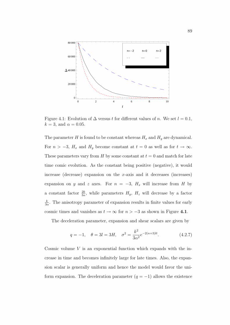
89

0 2 4 6 8 100

20 000

40 000

60 000

80 000

t

D

n=-2 n=0 n=2

Figure 4.1: Evolution of ∆ versus t for different values of n. We set l = 0.1,k = 3, and α = 0.05.

The parameter H is found to be constant whereas Hx and Hy are dynamical.

For n > −3, Hx and Hy become constant at t = 0 as well as for t → ∞.

These parameters vary from H by some constant at t = 0 and match for late

time comic evolution. As the constant being positive (negative), it would

increase (decrease) expansion on the x-axis and it decreases (increases)

expansion on y and z axes. For n = −3, Hx will increase from H by

a constant factor 2k3α

, while parameters Hy, Hz will decrease by a factor

k3α

. The anisotropy parameter of expansion results in finite values for early

cosmic times and vanishes as t →∞ for n > −3 as shown in Figure 4.1.

The deceleration parameter, expansion and shear scalars are given by

q = −1, θ = 3l = 3H, σ2 =k2

3α2e−2(n+3)lt. (4.2.7)

Cosmic volume V is an exponential function which expands with the in-

crease in time and becomes infinitely large for late times. Also, the expan-

sion scalar is generally uniform and hence the model would favor the uni-

form expansion. The deceleration parameter (q = −1) allows the existence

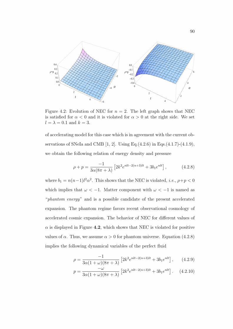
90

Ρ+p

0

2

4t

-6

-4

-2

Α

0.0

0.1

0.2

0.3

0.4

Ρ+p

0

2

4t

2

4

6

Α

-0.4

-0.3

-0.2

-0.1

0.0

Figure 4.2: Evolution of NEC for n = 2. The left graph shows that NECis satisfied for α < 0 and it is violated for α > 0 at the right side. We setl = λ = 0.1 and k = 3.

of accelerating model for this case which is in agreement with the current ob-

servations of SNeIa and CMB [1, 2]. Using Eq.(4.2.6) in Eqs.(4.1.7)-(4.1.9),

we obtain the following relation of energy density and pressure

ρ + p =−1

3α(8π + λ)

[2k2enlt−2(n+3)lt + 3b1e

nlt], (4.2.8)

where b1 = n(n−1)l2α2. This shows that the NEC is violated, i.e., ρ+p < 0

which implies that ω < −1. Matter component with ω < −1 is named as

“phantom energy” and is a possible candidate of the present accelerated

expansion. The phantom regime favors recent observational cosmology of

accelerated cosmic expansion. The behavior of NEC for different values of

α is displayed in Figure 4.2, which shows that NEC is violated for positive

values of α. Thus, we assume α > 0 for phantom universe. Equation (4.2.8)

implies the following dynamical variables of the perfect fluid

ρ =−1

3α(1 + ω)(8π + λ)

[2k2enlt−2(n+3)lt + 3b1e

nlt], (4.2.9)

p =−ω

3α(1 + ω)(8π + λ)

[2k2enlt−2(n+3)lt + 3b1e

nlt]. (4.2.10)

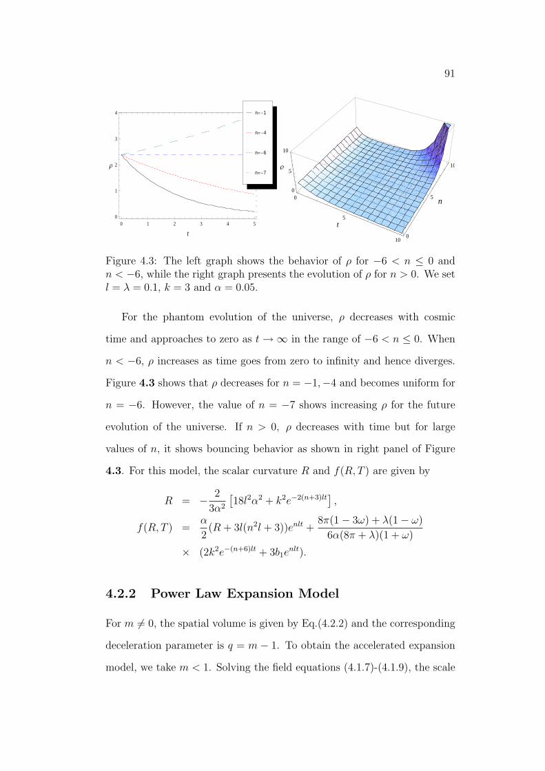
91

0 1 2 3 4 50

1

2

3

4

t

Ρ

n=-7

n=-6

n=-4

n=-1

0

5

10

t

0

5

10

n0

5

10

Ρ

Figure 4.3: The left graph shows the behavior of ρ for −6 < n ≤ 0 andn < −6, while the right graph presents the evolution of ρ for n > 0. We setl = λ = 0.1, k = 3 and α = 0.05.

For the phantom evolution of the universe, ρ decreases with cosmic

time and approaches to zero as t →∞ in the range of −6 < n ≤ 0. When

n < −6, ρ increases as time goes from zero to infinity and hence diverges.

Figure 4.3 shows that ρ decreases for n = −1,−4 and becomes uniform for

n = −6. However, the value of n = −7 shows increasing ρ for the future

evolution of the universe. If n > 0, ρ decreases with time but for large

values of n, it shows bouncing behavior as shown in right panel of Figure

4.3. For this model, the scalar curvature R and f(R, T ) are given by

R = − 2

3α2

[18l2α2 + k2e−2(n+3)lt

],

f(R, T ) =α

2(R + 3l(n2l + 3))enlt +

8π(1− 3ω) + λ(1− ω)

6α(8π + λ)(1 + ω)

× (2k2e−(n+6)lt + 3b1enlt).

4.2.2 Power Law Expansion Model

For m 6= 0, the spatial volume is given by Eq.(4.2.2) and the corresponding

deceleration parameter is q = m − 1. To obtain the accelerated expansion

model, we take m < 1. Solving the field equations (4.1.7)-(4.1.9), the scale

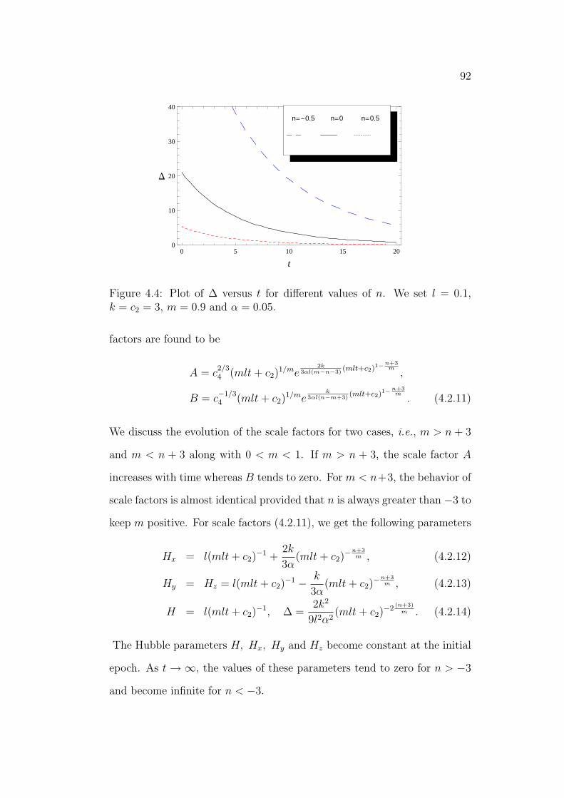
92

0 5 10 15 200

10

20

30

40

t

D

n=-0.5 n=0 n=0.5

Figure 4.4: Plot of ∆ versus t for different values of n. We set l = 0.1,k = c2 = 3, m = 0.9 and α = 0.05.

factors are found to be

A = c2/34 (mlt + c2)

1/me2k

3αl(m−n−3)(mlt+c2)1−

n+3m

,

B = c−1/34 (mlt + c2)

1/mek

3αl(n−m+3)(mlt+c2)1−

n+3m

. (4.2.11)

We discuss the evolution of the scale factors for two cases, i.e., m > n + 3

and m < n + 3 along with 0 < m < 1. If m > n + 3, the scale factor A

increases with time whereas B tends to zero. For m < n+3, the behavior of

scale factors is almost identical provided that n is always greater than −3 to

keep m positive. For scale factors (4.2.11), we get the following parameters

Hx = l(mlt + c2)−1 +

2k

3α(mlt + c2)

−n+3m , (4.2.12)

Hy = Hz = l(mlt + c2)−1 − k

3α(mlt + c2)

−n+3m , (4.2.13)

H = l(mlt + c2)−1, ∆ =

2k2

9l2α2(mlt + c2)

−2(n+3)

m . (4.2.14)

The Hubble parameters H, Hx, Hy and Hz become constant at the initial

epoch. As t → ∞, the values of these parameters tend to zero for n > −3

and become infinite for n < −3.

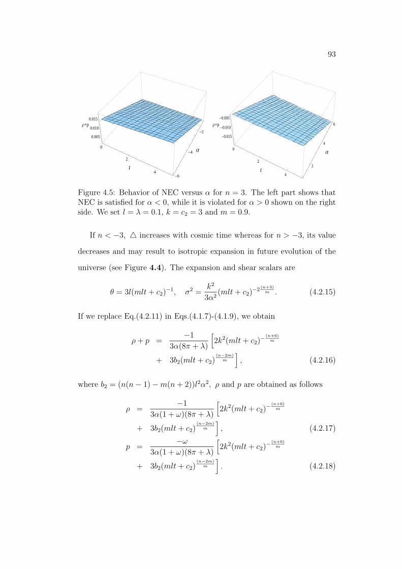
93

Ρ+p

0

2

4t

-6

-4

-2

Α

0.005

0.010

0.015 Ρ+p

0

2

4t

2

4

6

Α

-0.015

-0.010

-0.005

Figure 4.5: Behavior of NEC versus α for n = 3. The left part shows thatNEC is satisfied for α < 0, while it is violated for α > 0 shown on the rightside. We set l = λ = 0.1, k = c2 = 3 and m = 0.9.

If n < −3, 4 increases with cosmic time whereas for n > −3, its value

decreases and may result to isotropic expansion in future evolution of the

universe (see Figure 4.4). The expansion and shear scalars are

θ = 3l(mlt + c2)−1, σ2 =

k2

3α2(mlt + c2)

−2(n+3)

m . (4.2.15)

If we replace Eq.(4.2.11) in Eqs.(4.1.7)-(4.1.9), we obtain

ρ + p =−1

3α(8π + λ)

[2k2(mlt + c2)

− (n+6)m

+ 3b2(mlt + c2)(n−2m)

m

], (4.2.16)

where b2 = (n(n− 1)−m(n + 2))l2α2, ρ and p are obtained as follows

ρ =−1

3α(1 + ω)(8π + λ)

[2k2(mlt + c2)

− (n+6)m

+ 3b2(mlt + c2)(n−2m)

m

], (4.2.17)

p =−ω

3α(1 + ω)(8π + λ)

[2k2(mlt + c2)

− (n+6)m

+ 3b2(mlt + c2)(n−2m)

m

]. (4.2.18)

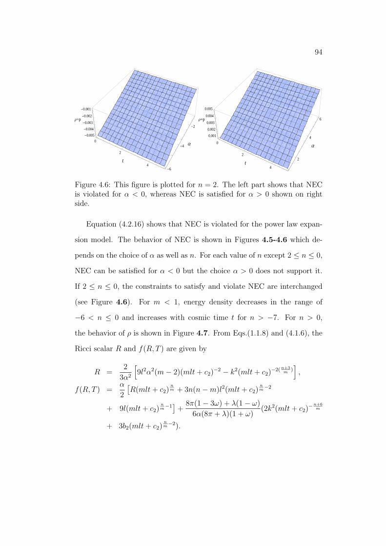
94

Ρ+p

0

2

4t

-6

-4

-2

Α

-0.005

-0.004

-0.003

-0.002

-0.001

Ρ+p

0

2

4t

2

4

6

Α

0.001

0.002

0.003

0.004

0.005

Figure 4.6: This figure is plotted for n = 2. The left part shows that NECis violated for α < 0, whereas NEC is satisfied for α > 0 shown on rightside.

Equation (4.2.16) shows that NEC is violated for the power law expan-

sion model. The behavior of NEC is shown in Figures 4.5-4.6 which de-

pends on the choice of α as well as n. For each value of n except 2 ≤ n ≤ 0,

NEC can be satisfied for α < 0 but the choice α > 0 does not support it.

If 2 ≤ n ≤ 0, the constraints to satisfy and violate NEC are interchanged

(see Figure 4.6). For m < 1, energy density decreases in the range of

−6 < n ≤ 0 and increases with cosmic time t for n > −7. For n > 0,

the behavior of ρ is shown in Figure 4.7. From Eqs.(1.1.8) and (4.1.6), the

Ricci scalar R and f(R, T ) are given by

R =2

3α2

[9l2α2(m− 2)(mlt + c2)

−2 − k2(mlt + c2)−2(n+3

m)],

f(R, T ) =α

2

[R(mlt + c2)

nm + 3n(n−m)l2(mlt + c2)

nm−2

+ 9l(mlt + c2)nm−1

]+

8π(1− 3ω) + λ(1− ω)

6α(8π + λ)(1 + ω)(2k2(mlt + c2)

−n+6m

+ 3b2(mlt + c2)nm−2).

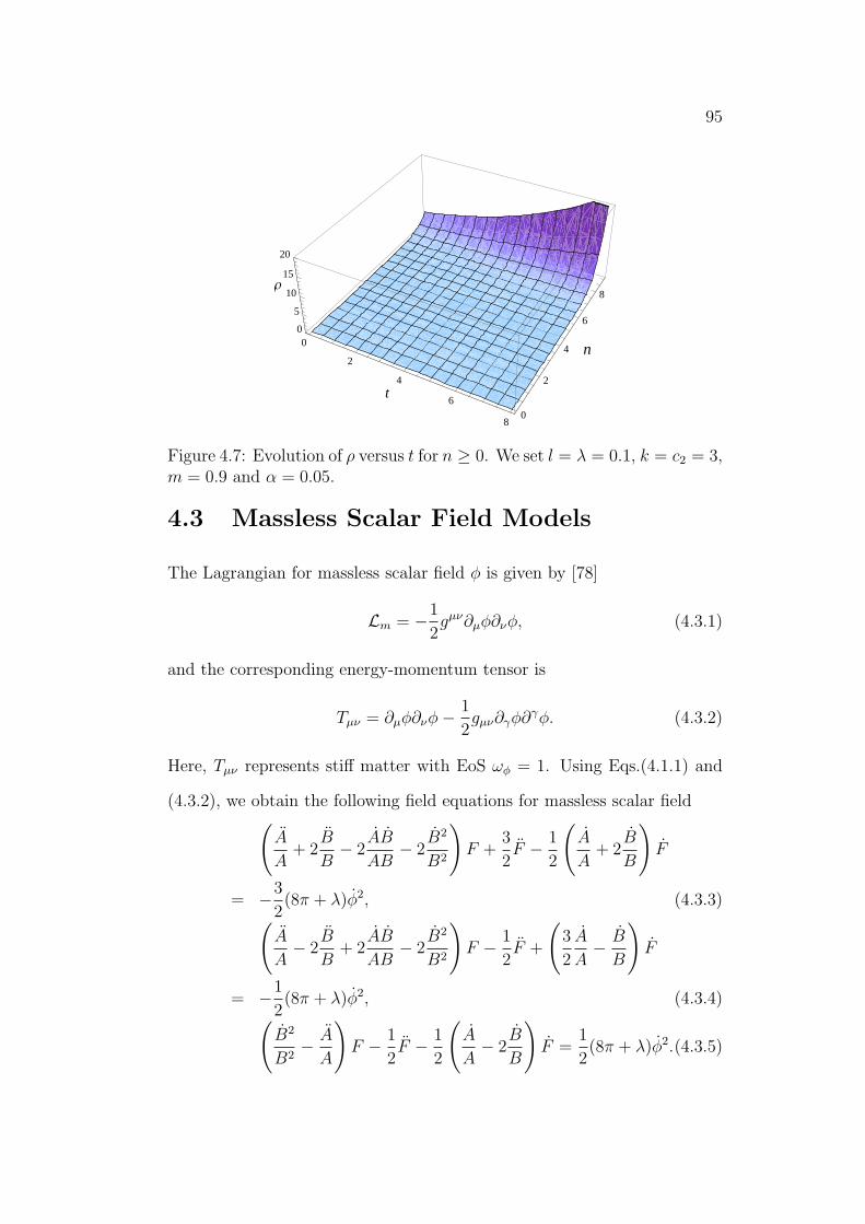
95

0

2

4

6

8

t

0

2

4

6

8

n

0

5

10

15

20

Ρ

Figure 4.7: Evolution of ρ versus t for n ≥ 0. We set l = λ = 0.1, k = c2 = 3,m = 0.9 and α = 0.05.

4.3 Massless Scalar Field Models

The Lagrangian for massless scalar field φ is given by [78]

Lm = −1

2gµν∂µφ∂νφ, (4.3.1)

and the corresponding energy-momentum tensor is

Tµν = ∂µφ∂νφ− 1

2gµν∂γφ∂γφ. (4.3.2)

Here, Tµν represents stiff matter with EoS ωφ = 1. Using Eqs.(4.1.1) and

(4.3.2), we obtain the following field equations for massless scalar field(

A

A+ 2

B

B− 2

AB

AB− 2

B2

B2

)F +

3

2F − 1

2

(A

A+ 2

B

B

)F

= −3

2(8π + λ)φ2, (4.3.3)

(A

A− 2

B

B+ 2

AB

AB− 2

B2

B2

)F − 1

2F +

(3

2

A

A− B

B

)F

= −1

2(8π + λ)φ2, (4.3.4)

(B2

B2− A

A

)F − 1

2F − 1

2

(A

A− 2

B

B

)F =

1

2(8π + λ)φ2.(4.3.5)

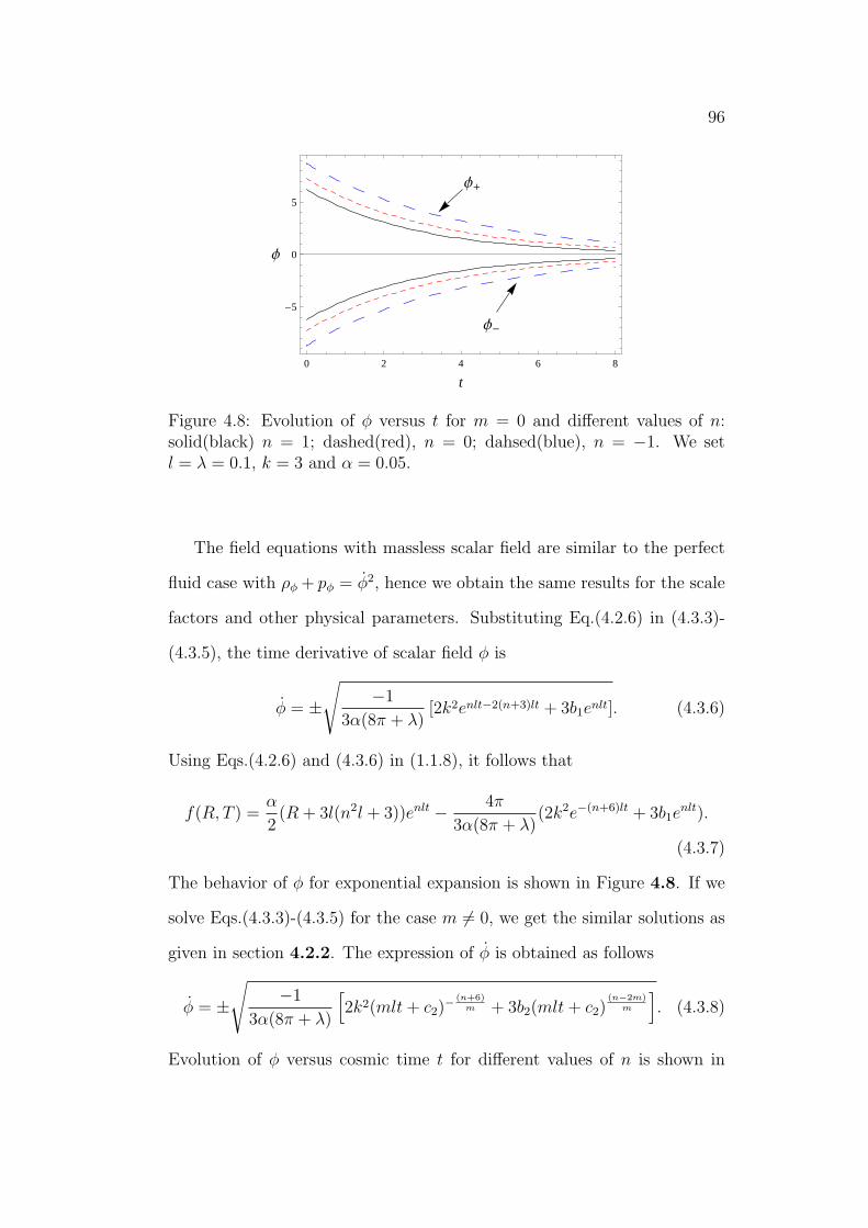
96

Φ+

Φ-

0 2 4 6 8

-5

0

5

t

Φ

Figure 4.8: Evolution of φ versus t for m = 0 and different values of n:solid(black) n = 1; dashed(red), n = 0; dahsed(blue), n = −1. We setl = λ = 0.1, k = 3 and α = 0.05.

The field equations with massless scalar field are similar to the perfect

fluid case with ρφ + pφ = φ2, hence we obtain the same results for the scale

factors and other physical parameters. Substituting Eq.(4.2.6) in (4.3.3)-

(4.3.5), the time derivative of scalar field φ is

φ = ±√

−1

3α(8π + λ)[2k2enlt−2(n+3)lt + 3b1enlt]. (4.3.6)

Using Eqs.(4.2.6) and (4.3.6) in (1.1.8), it follows that

f(R, T ) =α

2(R + 3l(n2l + 3))enlt − 4π

3α(8π + λ)(2k2e−(n+6)lt + 3b1e

nlt).

(4.3.7)

The behavior of φ for exponential expansion is shown in Figure 4.8. If we

solve Eqs.(4.3.3)-(4.3.5) for the case m 6= 0, we get the similar solutions as

given in section 4.2.2. The expression of φ is obtained as follows

φ = ±√

−1

3α(8π + λ)

[2k2(mlt + c2)

− (n+6)m + 3b2(mlt + c2)

(n−2m)m

]. (4.3.8)

Evolution of φ versus cosmic time t for different values of n is shown in

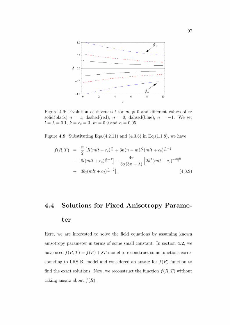
97

Φ+

Φ-0 2 4 6 8 10

-1.0

-0.5

0.0

0.5

1.0

t

Φ

Figure 4.9: Evolution of φ versus t for m 6= 0 and different values of n:solid(black) n = 1; dashed(red), n = 0; dahsed(blue), n = −1. We setl = λ = 0.1, k = c2 = 3, m = 0.9 and α = 0.05.

Figure 4.9. Substituting Eqs.(4.2.11) and (4.3.8) in Eq.(1.1.8), we have

f(R, T ) =α

2

[R(mlt + c2)

nm + 3n(n−m)l2(mlt + c2)

nm−2

+ 9l(mlt + c2)nm−1

]− 4π

3α(8π + λ)

[2k2(mlt + c2)

−n+6m

+ 3b2(mlt + c2)nm−2

]. (4.3.9)

4.4 Solutions for Fixed Anisotropy Parame-

ter

Here, we are interested to solve the field equations by assuming known

anisotropy parameter in terms of some small constant. In section 4.2, we

have used f(R, T ) = f(R)+λT model to reconstruct some functions corre-

sponding to LRS BI model and considered an ansatz for f(R) function to

find the exact solutions. Now, we reconstruct the function f(R, T ) without

taking ansatz about f(R).

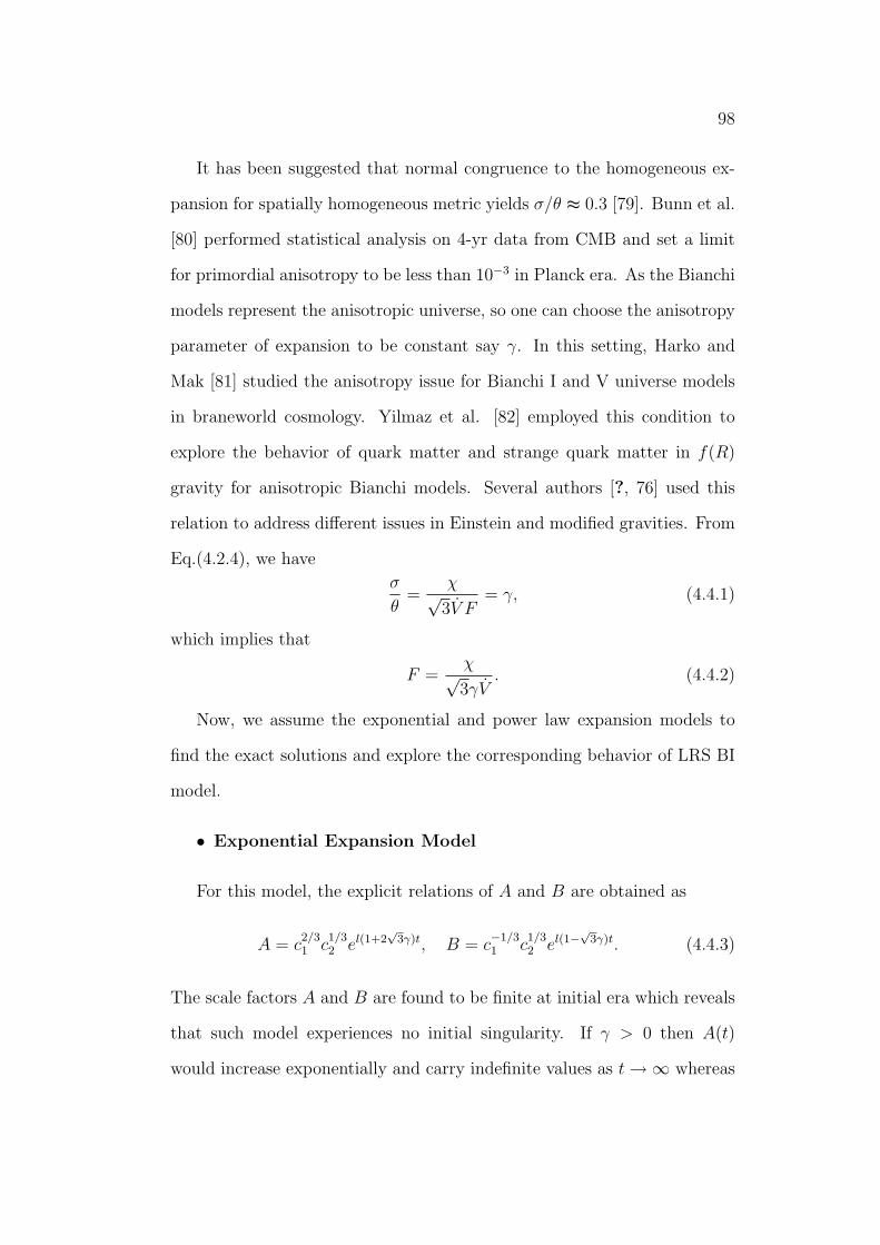
98

It has been suggested that normal congruence to the homogeneous ex-

pansion for spatially homogeneous metric yields σ/θ ≈ 0.3 [79]. Bunn et al.

[80] performed statistical analysis on 4-yr data from CMB and set a limit

for primordial anisotropy to be less than 10−3 in Planck era. As the Bianchi

models represent the anisotropic universe, so one can choose the anisotropy

parameter of expansion to be constant say γ. In this setting, Harko and

Mak [81] studied the anisotropy issue for Bianchi I and V universe models

in braneworld cosmology. Yilmaz et al. [82] employed this condition to

explore the behavior of quark matter and strange quark matter in f(R)

gravity for anisotropic Bianchi models. Several authors [?, 76] used this

relation to address different issues in Einstein and modified gravities. From

Eq.(4.2.4), we have

σ

θ=

χ√3V F

= γ, (4.4.1)

which implies that

F =χ√3γV

. (4.4.2)

Now, we assume the exponential and power law expansion models to

find the exact solutions and explore the corresponding behavior of LRS BI

model.

• Exponential Expansion Model

For this model, the explicit relations of A and B are obtained as

A = c2/31 c

1/32 el(1+2

√3γ)t, B = c

−1/31 c

1/32 el(1−√3γ)t. (4.4.3)

The scale factors A and B are found to be finite at initial era which reveals

that such model experiences no initial singularity. If γ > 0 then A(t)

would increase exponentially and carry indefinite values as t →∞ whereas

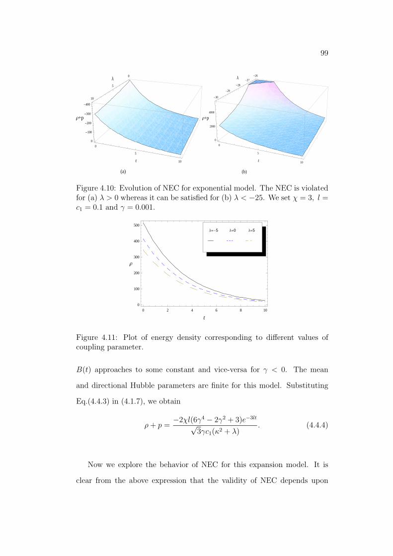
99

Ρ+p

0

5

10t

0

5

10

Λ

-400

-300

-200

-100

0

(a)

Ρ+p

0

5

10t

-30

-29

-28

-27

-26Λ

0

2000

4000

(b)

Figure 4.10: Evolution of NEC for exponential model. The NEC is violatedfor (a) λ > 0 whereas it can be satisfied for (b) λ < −25. We set χ = 3, l =c1 = 0.1 and γ = 0.001.

0 2 4 6 8 100

100

200

300

400

500

t

Ρ

Λ=-5 Λ=0 Λ=5

Figure 4.11: Plot of energy density corresponding to different values ofcoupling parameter.

B(t) approaches to some constant and vice-versa for γ < 0. The mean

and directional Hubble parameters are finite for this model. Substituting

Eq.(4.4.3) in (4.1.7), we obtain

ρ + p =−2χl(6γ4 − 2γ2 + 3)e−3lt

√3γc1(κ2 + λ)

. (4.4.4)

Now we explore the behavior of NEC for this expansion model. It is

clear from the above expression that the validity of NEC depends upon

100

the constants χ, l, c1, γ and coupling parameter λ. Since constants other

than λ are selected as positive, so we examine the NEC depending upon the

values of parameter λ. If λ > 0 then NEC is violated so that EoS parameter

< −1 which is shown in Figure 4.10(a). The candidate of exotic matter

corresponding to ω < −1 is termed as phantom energy and is responsible

for the present accelerating phase which favors the current observational

data [1, 2]. The NEC can be met only if the denominator of the above

relation is negative which is shown in Figure 4.10(b). The energy density is

plotted for different values of coupling parameter λ in the spirit of phantom

regime. Figure 4.11 shows that energy density is a decreasing function of

cosmic time. Substituting Eqs.(4.4.2) and (4.4.3) in (1.1.8), one can get the

expression of f(R, T ) for the above model

f(R, T ) =χe−3lt

6√

3γc1l(9l(3l + 1)−R) +

χe−3lt

√3γ(κ2 + λ)(1 + ω)c1

l(6γ4

− 2γ2 + 3)(κ2(1− 3ω) + λ(1 + ω)). (4.4.5)

• Power Law Expansion Model

We take power law expansion model defined by the scale factor a(t) =

(mlt + c3)1/m and deceleration parameter q = m− 1. This universe model

favors the accelerated expansion for 0 < m < 1 whereas for m > 1, it

describes the decelerating phase. Solving the field equations, we get the

scale factors as

A = c2/31 (mlt + c3)

1+2√

3γm , B = c

−1/31 (mlt + c3)

1−√3γm . (4.4.6)

At the present era, these scale factors are finite while in future epoch the

evolution of A and B depends upon constant γ. Using Eq.(4.4.6), we obtain

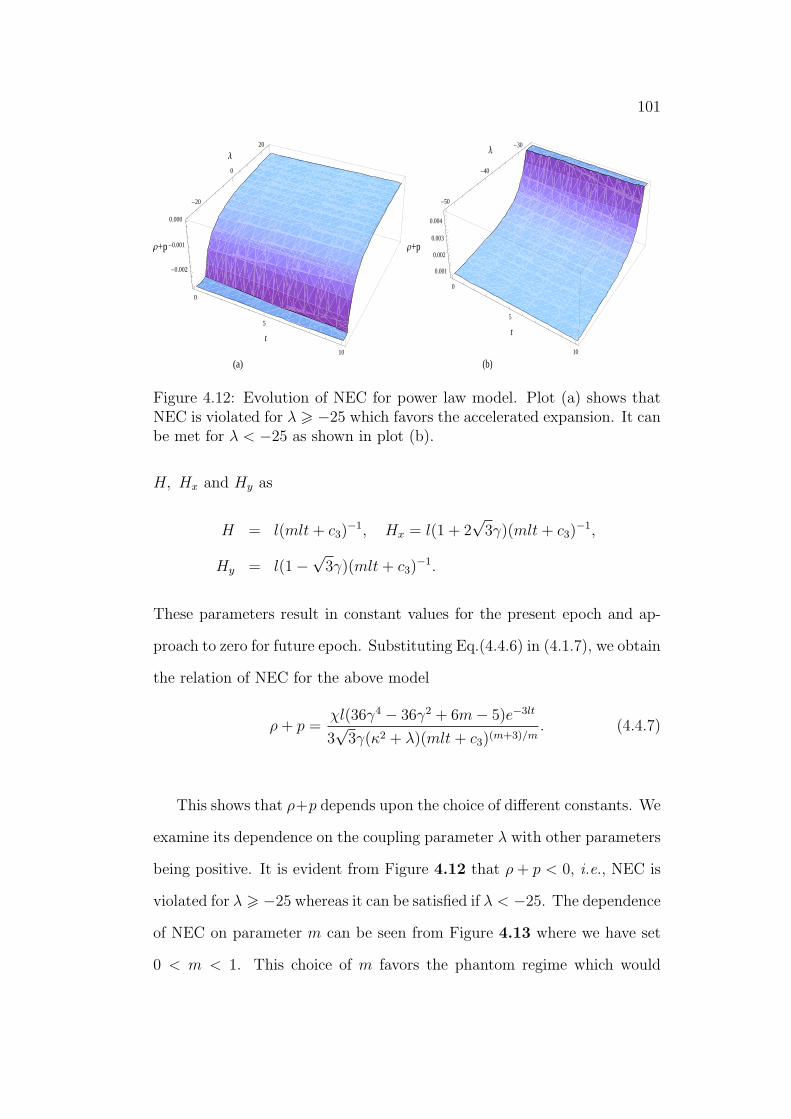
101

Ρ+p

0

5

10

t

-20

0

20

Λ

-0.002

-0.001

0.000

(a)

Ρ+p

0

5

10

t

-50

-40

-30Λ

0.001

0.002

0.003

0.004

(b)

Figure 4.12: Evolution of NEC for power law model. Plot (a) shows thatNEC is violated for λ > −25 which favors the accelerated expansion. It canbe met for λ < −25 as shown in plot (b).

H, Hx and Hy as

H = l(mlt + c3)−1, Hx = l(1 + 2

√3γ)(mlt + c3)

−1,

Hy = l(1−√

3γ)(mlt + c3)−1.

These parameters result in constant values for the present epoch and ap-

proach to zero for future epoch. Substituting Eq.(4.4.6) in (4.1.7), we obtain

the relation of NEC for the above model

ρ + p =χl(36γ4 − 36γ2 + 6m− 5)e−3lt

3√

3γ(κ2 + λ)(mlt + c3)(m+3)/m. (4.4.7)

This shows that ρ+p depends upon the choice of different constants. We

examine its dependence on the coupling parameter λ with other parameters

being positive. It is evident from Figure 4.12 that ρ + p < 0, i.e., NEC is

violated for λ > −25 whereas it can be satisfied if λ < −25. The dependence

of NEC on parameter m can be seen from Figure 4.13 where we have set

0 < m < 1. This choice of m favors the phantom regime which would

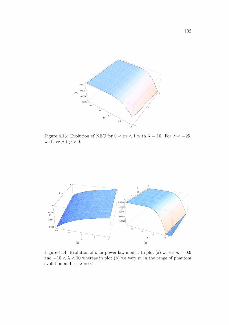
102

Ρ+p 0

5

10

t

0.2

0.4

0.6

0.8

1.0

m

-0.0006

-0.0004

-0.0002

0.0000

Figure 4.13: Evolution of NEC for 0 < m < 1 with λ = 10. For λ < −25,we have ρ + p > 0.

0

5

10

t

-10-5

05

10Λ

0.0004

0.0006

0.0008

Ρ

(a)

0

5

10

15

20t

0.2

0.4

0.6

0.8m

0.00000

0.00005

0.00010

0.00015

0.00020

Ρ

(b)

Figure 4.14: Evolution of ρ for power law model. In plot (a) we set m = 0.9and −10 < λ < 10 whereas in plot (b) we vary m in the range of phantomevolution and set λ = 0.1

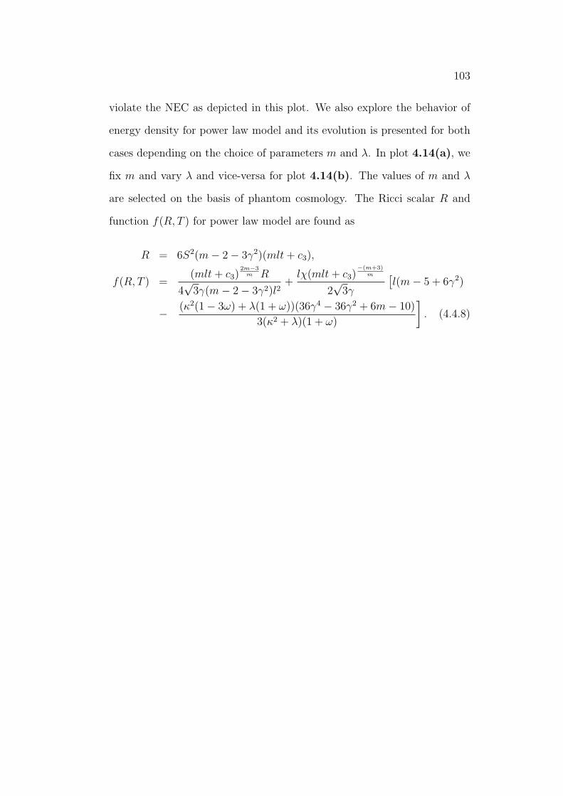
103

violate the NEC as depicted in this plot. We also explore the behavior of

energy density for power law model and its evolution is presented for both

cases depending on the choice of parameters m and λ. In plot 4.14(a), we

fix m and vary λ and vice-versa for plot 4.14(b). The values of m and λ

are selected on the basis of phantom cosmology. The Ricci scalar R and

function f(R, T ) for power law model are found as

R = 6S2(m− 2− 3γ2)(mlt + c3),

f(R, T ) =(mlt + c3)

2m−3m R

4√

3γ(m− 2− 3γ2)l2+

lχ(mlt + c3)−(m+3)

m

2√

3γ

[l(m− 5 + 6γ2)

− (κ2(1− 3ω) + λ(1 + ω))(36γ4 − 36γ2 + 6m− 10)

3(κ2 + λ)(1 + ω)

]. (4.4.8)

Chapter 5

Discussion and Conclusion

The late time accelerated cosmic expansion is a major issue in cosmology.

Modified theories of gravity have appeared as convenient candidates to ad-

dress such issues and predict the destiny of the universe. Theories involving

CMC have attained significant importance to explore the enigma of cosmic

evolution and other cosmological aspects. In this setting, f(R, T ) gravity

can be reckoned as an effective campaigner of dark components with no

need of introducing either the existence of extra spatial dimension or an

exotic component of DE. Such theory is of great importance as the source

of DE components can be seen from an integrated contribution of both cur-

vature and matter Lagrangian parts. The matter geometry coupling results

in existence of extra force due to non-geodesic motion of test particles.

f(R, T,Q) is another more general modified gravity formulated on the

basis of CMC. This theory involves the contraction of Ricci tensor and mater

energy-momentum tensor Q = RµνTµν and can be regarded as an extended

form of f(R, T ) gravity. However, there is a significant difference in the

results of this theory with the rest of modifications. For instance, if one

considers the role of electromagnetic field or radiation dominated fluid (i.e.,

trace free energy-momentum tensor), the field equations in f(R, T ) gravity

104

105

reduce to that in f(R) gravity. Thus, the contribution of non-minimal

coupling would disappear in f(R, T ) gravity whereas in f(R, T,Q) gravity,

the effect of non-minimal coupling can be assured due to the contribution of

contraction term Q. Indeed, in Lagrangian (1.1.15) the interaction between

matter and geometry can be seen through the coupling of energy-momentum

and Ricci tensors, Q is the generic term responsible for the non-minimal

coupling as compared to other modified theories. Such behavior becomes

more explicit for the models of the type R + αQ and R(1 + αQ). However,

still one can formulate more complex models and discuss the cosmological

features.

In fact, the fundamental characteristic of theories involving non-minimal

matter geometry coupling is the non-conserved energy-momentum tensor

produced from the divergence of the field equations. As a result, motion of

test particles is non-geodesic and an extra force orthogonal to four-velocity

of the particle is present due to matter geometry coupling. This is consistent

with the interpretation of four force which states that component of force

orthogonal to particle’s four-velocity can influence its trajectory. It has

been shown that the extra force vanishes if one uses the matter Lagrangian

of the form Lm = p [83] for non-minimally coupled f(R) theories (as given

in [84, 85]). However, the extra force generated by the matter geometry

coupling does not vanish in this modified theory even for Lm = p. It also

involves the contribution from the Ricci tensor and may lead to significant

deviation from the geodesic paths. The extra force can be useful to explain

the DM properties and Pioneer anomaly. One can count the additional

curvature obtained from the CMC to inform the galactic rotation curves.

This theory can also present novel views about the early stages of cosmic

106

evolution specifically the inflationary paradigm.

In this thesis, we have discussed the thermodynamic laws at the AH of

FRW universe for f(R, T ) and f(R, T,Q) theories. In particular, we have

presented the non-equilibrium description of thermodynamics and explored

the existence of equilibrium picture. We have also addressed the question

how to constrain the various forms of Lagrangian in these theories on phys-

ical grounds employing the energy conditions and test the stability criteria.

The anisotropic universe models are also discussed to present the cosmic

evolution and reconstruct the corresponding form of Lagrangian. The sig-

nificant findings have been listed below.

In Chapter 2, it is shown that the representation of equilibrium thermo-

dynamics is not executable in f(R, T ) theory. Thus, the non-equilibrium

treatment of thermodynamics is used to discuss the laws of thermodynam-

ics. The FLT is formulated by using the Wald’s entropy relation. It is

found that additional entropy term is produced as a result of CMC. The

gravitational coupling between matter and higher derivative terms of cur-

vature describes a transfer of energy and momentum across the horizon

which can be the explanation for non-equilibrium picture. It is worth

mentioning here that no such term is present in Einstein, Gauss-Bonnet,

Lovelock and braneworld modified theories [19]-[54]. The equilibrium and

non-equilibrium descriptions of thermodynamics in f(R) gravity can be re-

produced from these results.

We have also explored the validity of GSLT at the AH of FRW uni-

verse in this modified theory. The time evolution of entropy Stot (contribu-

tions from horizon entropy and entropy associated with the matter contents

within the horizon) is presented in a comprehensive way. We have assumed

107

the proportionality relation between the temperatures related to AH and

matter components inside the horizon. The condition Tin = bTh relates the

temperature of ingredients inside the horizon to the temperature of AH.

We adopt the proposal of thermal equilibrium and set b = 1 to explore the

validity of GSLT. It is concluded that GSLT is satisfied in both phantom

and quintessence regimes of the universe.

In f(R, T,Q) gravity, the general formalism of the field equations for

FRW spacetime with any spatial curvature is presented. It is shown that

these equations can be cast to the form of FLT, ThdSh + ThdS = δQ, in

non-equilibrium description of thermodynamics. In this structure of FLT,

we have found that entropy Seff = Sh + S involves contribution from two

factors, the first corresponds to horizon entropy in terms of area and sec-

ond represents the entropy production term dS which is produced due to

the non-equilibrium description in f(R, T,Q) gravity. This shows that one

may need the non-equilibrium treatment of thermodynamics in this the-

ory. The entropy production term in f(R, T,Q) gravity is more general

and can reproduce the corresponding factor in f(R) and f(R, T ) theories.

This modified theory involves strong coupling resulting from the contrac-

tion of Ricci tensor and matter energy-momentum tensor. Due to this

interaction, the entropy production term would be ultimate in f(R, T,Q)

gravity. Different schemes have been suggested to avoid the auxiliary term

in FLT [21, 23, ?, 86] in f(R) and scalar-tensor theories. Bamba et al.

[21, 23] showed that one can redefine the energy-momentum tensor contri-

bution from the modified theories so that the conservation equation is truly

satisfied and hence leads to the omission of entropy production term. How-

ever, we have seen that such procedure is not fruitful in f(R, T ) theory and

108

equilibrium thermodynamics needs more study to follow. Since f(R, T,Q)

gravity is a more general theory, so the non-equilibrium representation of

thermodynamics is shown in the present work.

In order to get insights of GSLT in thermal equilibrium, we have taken

two specific gravitational models and developed the constraints for the ac-

celerated cosmic expansion with m > 1. We have found that for flat FRW

universe in power law cosmology, the validity of GSLT depends upon the

coupling parameter α as shown in Figures 2.1-2.2. The viability constraints

are given as follows:

• f(R, T,Q) = R + αQ,

If Lm = −p then GSLT is satisfied for α < 0, m > 1.

If Lm = ρ then GSLT is satisfied for α < 0, m > 8.

• f(R, T,Q) = R(1 + αQ),

For Lm = −p, GSLT is satisfied for α > 0, m > 1.

For Lm = ρ, GSLT is satisfied for α > 0, m > 3.

We have also considered the Lagrangian f(R, T,Q) = R + f(Q) + G(T )

[14] to validate the GSLT in de Sitter background and results are shown

in Figure 2.3. Thus, we have presented the validity of GSLT in expanding

universe with the assumption of thermal equilibrium which may be achieved

in later times. Finally, we conclude that our study on non-equilibrium

thermodynamics in f(R, T ) and f(R, T,Q) gravity is consistent with the

statements given in [20, 55, 21, 23].

Chapter 3 presents the energy conditions constraints and stability of

f(R, T ) and f(R, T,Q) theories. Lagrangian of f(R, T,Q) gravity is more

109

comprehensive implying that different functional forms of f can be sug-

gested. The versatility in Lagrangian raises the question that how to con-

strain such a theory on physical grounds. We have developed some con-

straints for general as well as specific forms of f(R, T,Q) gravity by exam-

ining the respective energy conditions. The NEC and SEC are derived using

the Raychaudhuri equation along with the condition that gravity is attrac-

tive. Moreover, these inequalities are equivalent to the results found from

conditions ρ + 3p > 0 and ρ + p > 0 under the transformations ρ → ρeff

and p → peff , respectively. One can employ the similar procedure to derive

the WEC and DEC by translating their counterpart in GR for effective

energy-momentum tensor. The conditions of positive effective gravitational

coupling and attractive nature of gravity are also obtained in this theory.

To illustrate how these conditions can constrain the f(R, T,Q) gravity,

we have taken two functional forms of f namely, f = R + αQ and f =

R(1 + αQ). It is shown that WEC for these models depends upon the

coupling parameter α which is satisfied only if α is negative. We have also

set the Dolgov-Kawasaki criterion in this discussion. The f(R, T ) gravity

is addressed as a specific case to this modified theory. We have taken two

interesting choices for the Lagrangian, one involving an exponential function

and other having explicit coupling between R and T . The validity of WEC

for both choices of matter Lagrangian Lm = p and Lm = −ρ have been

explored. The WEC for f(R, T ) = αexp(

Rα

+ λT)

is met in both cases if

coupling parameter λ > 0 and α > 2H20 (j0−q0−2)(or α > 4H2

0 (j0−q0−2)),

respectively. For the model f(R, T ) = R + ηRmT n, the WEC is satisfied if

both the constants m and n are positive.

We have discussed the power law solutions for two particular cases and

110

derived the corresponding energy bounds. We summarize the results of

these two models as follows.

• f(R) + λT

It is shown that exact power law solution exists for this form of f(R, T )

gravity given in Eq.(3.3.21). In the limit of λ = 0, the corresponding result

can be recovered in f(R) gravity. To ensure that this theory reduces to GR,

we need to set C1 = C2 = λ = 0 with m = 23(1+ω)

and ρ0 = 43(1+ω)2

. We have

constructed the general form of f(R) + λT model which corresponds to Rn

gravity. For this particular model, we have examined the WEC bounds in

terms of present day observational values H0, q0, j0 and s0.

• R + 2f(T )

A general form of f(T ) model (3.3.31) is obtained which corresponds

to GR in the limit n = 1. We have applied the energy conditions to set

the possible constraints on this f(R, T ) model. It is found that energy

conditions are globally satisfied within the range of n = −1, 2, 3, .... It

is worth mentioning here that results of power law solutions and energy

conditions found here are quite general which correspond to GR and f(R)

gravity.

We have also analyzed the stability of power law solutions under linear

homogeneous perturbations in the FRW background for f(R, T ) gravity. In

particular, perturbations for energy density and Hubble parameter are in-

troduced which produce linearized perturbed field equations. The stability

conditions are found to be compatible with energy conditions bounds to

some extent. Hence, power law solutions in f(R, T ) gravity can be consid-

ered as viable models to explain the cosmic expansion history.

111

Chapter 4 investigates the homogeneous but not necessarily isotropic

models in the context of f(R, T ) gravity. We have employed the f(R, T ) =

f(R) + λT choice to reconstruct some explicit models of f(R, T ) gravity

for LRS BI universe. The exact solutions of the modified field equations

are obtained for the LRS BI universe with perfect fluid and massless scalar

field. The law of variation of mean Hubble parameter is assumed implying

two cosmological models for m = 0 and m 6= 0 which support the recent

observations about the accelerated cosmic expansion. We have presented

physical properties as well as kinematical parameters of the models. In the

following, we summarize the results for these two models.

(i) Model for V = c1e3lt

For exponential expansion model, the accelerated expansion of the universe

may occur as q = −1. The kinematical parameters have been discussed for

two cases n > −3 and n < −3. The expansion scalar is constant, while the

Ricci scalar approaches to constant value as t → ∞ for n > −3 and take

infinitely large values for n < −3. The anisotropy parameter of expansion

depends upon time and vanishes in future evolution for n > −3. If α > 0,

NEC is violated. We are not able to find the explicit function of f(R, T )

by using Eq.(1.1.8). For λ = 0, we develop f(R) in terms of R and hence

the function f(R, T ) as

f(R) =

[2αω

1 + ω(R + 12H2) +

1

2α3α2H((n2 − 4)H + 3) +

1− 3ω

1 + ωb1

]enlt,

which can be expressed as

f(R1) = const1 ×R1m1 + const2 ×R1

m2 ,

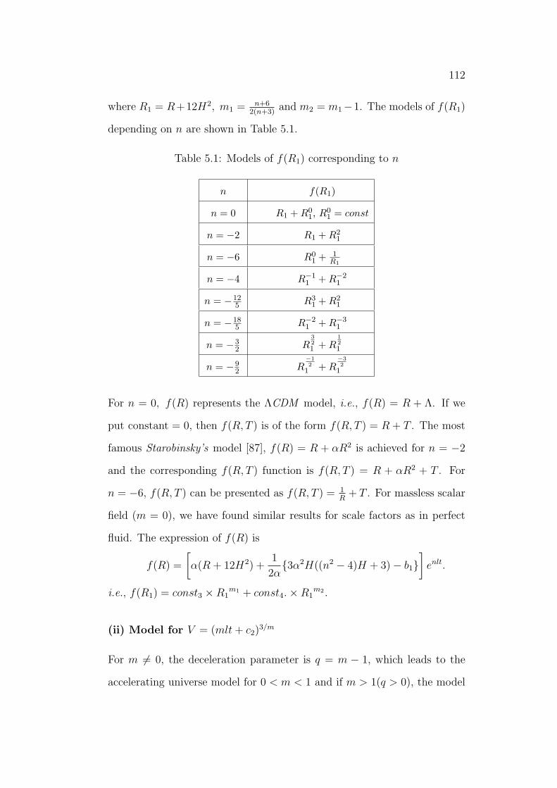
112

where R1 = R+12H2, m1 = n+62(n+3)

and m2 = m1−1. The models of f(R1)

depending on n are shown in Table 5.1.

Table 5.1: Models of f(R1) corresponding to n

n f(R1)

n = 0 R1 + R01, R0

1 = const

n = −2 R1 + R21

n = −6 R01 + 1

R1

n = −4 R−11 + R−2

1

n = −125 R3

1 + R21

n = −185 R−2

1 + R−31

n = −32 R

321 + R

121

n = −92 R

−12

1 + R−32

1

For n = 0, f(R) represents the ΛCDM model, i.e., f(R) = R + Λ. If we

put constant = 0, then f(R, T ) is of the form f(R, T ) = R + T . The most

famous Starobinsky’s model [87], f(R) = R + αR2 is achieved for n = −2

and the corresponding f(R, T ) function is f(R, T ) = R + αR2 + T . For

n = −6, f(R, T ) can be presented as f(R, T ) = 1R

+ T . For massless scalar

field (m = 0), we have found similar results for scale factors as in perfect

fluid. The expression of f(R) is

f(R) =

[α(R + 12H2) +

1

2α3α2H((n2 − 4)H + 3)− b1

]enlt.

i.e., f(R1) = const3 ×R1m1 + const4.×R1

m2 .

(ii) Model for V = (mlt + c2)3/m

For m 6= 0, the deceleration parameter is q = m − 1, which leads to the

accelerating universe model for 0 < m < 1 and if m > 1(q > 0), the model

113

represents decelerating phase of the universe. The evolution of the scale

factors is discussed for two cases m > n+3 and m < n+3 with 0 < m < 1.

The anisotropy parameter of expansion increases for n < −3, whereas it

may result in isotropic expansion in future evolution of the universe for

n > −3. The Hubble parameter, expansion scalar and shear scalar approach

to constant at earlier times of the universe and tend to zero as t →∞. The

scalar curvature R becomes constant as t → ∞ for n > −3, whereas it

diverges for n < −3. When λ = 0, we have

f(R) = (mlt + c2)n/m

[2αω

1 + ω(R− 6(m− 2)H2) +

α

2H3H(n2

+ m− 4) +1− 3ω

α2l2(1 + ω)b2H + 9

],

which leads to

f(R2) = const5 ×R2m1 + const6 ×R2

m2 ,

where R2 = R− 6(m− 2)H2. In case of massless scalar field, f(R) is

f(R) = (mlt + c2)n/m

[α(R− 6(m− 2)H2) +

α

2H3H(n2 + m

− 4) +b2H

α2l2+ 9

],

i.e., f(R2) = const7 × R2m1 + const8 × R2

m2 . We have seen that all f(R)

represent identical behavior with different constraints. The NEC is found

to be violated for both models m = 0 and m 6= 0 which results in phantom

evolution. For ω < −1, energy density is found to be positive and pressure

is negative. Thus, our solutions for perfect fluid represent the phantom era

of DE. The isotropic behavior of models is observed for future evolution.

Although the anisotropy of CMB is restricted on cosmological scales

114

which can favor the FRW universe but allowing local anisotropy while pre-

serving isotropic expansion dynamics is possible at least on phenomenolog-

ical level. However, in section 4.4 we have considered that the deviations

from isotropy are small, and we have restricted our analysis to ansatz that

anisotropy parameter of expansion ∆ being small constant. We have dis-

cussed the above models in this setting. We have examined the evolution

of NEC counting the value of coupling parameter λ for model (i). For

λ > 0, NEC is violated resulting in EoS parameter ω < −1 which can be

met if λ < −25. The energy density turns out to be constant at present

era and gets smaller values depending on time. For exponential model, the

expression of f(R, T ) is given

f(R, T ) =χe−3lt

6√

3γc1l(9l(3l + 1)−R) +

χe−3lt

√3γ(κ2 + λ)(1 + ω)c1

l(6γ4

− 2γ2 + 3)(κ2(1− 3ω) + λ(1 + ω)).

The above expression depends upon R as well as exponential function of

time t which is due to scale factors but still one can represent the above

expression in terms of R and T .

From Eq.(4.4.4), we represent e−3lt in terms of T as

e−3lt = C1T, C1 =(1 + ω)

√3γc1(κ

2 + λ)

2lχ(1− 3ω)(2γ2 − 6γ4 − 3),

so that f(R, T ) is given by

f(R, T ) = α1T + α2RT.

For case (ii), we have explored the validity of NEC for both cases depending

on coupling parameter λ and m. For λ, the situation is similar to that for

exponential model and NEC is violated for 0 < m < 1 with λ > −25. In

this case, we can construct some explicit f(R, T ) models. For this purpose,

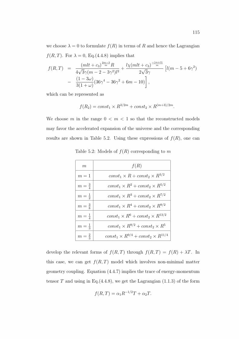
115

we choose λ = 0 to formulate f(R) in terms of R and hence the Lagrangian

f(R, T ). For λ = 0, Eq.(4.4.8) implies that

f(R, T ) =(mlt + c3)

2m−3m R

4√

3γ(m− 2− 3γ2)l2+

lχ(mlt + c3)−(m+3)

m

2√

3γ

[l(m− 5 + 6γ2)

− (1− 3ω)

3(1 + ω)(36γ4 − 36γ2 + 6m− 10)

],

which can be represented as

f(R2) = const1 ×R3/2m + const2 ×R(m+3)/2m.

We choose m in the range 0 < m < 1 so that the reconstructed models

may favor the accelerated expansion of the universe and the corresponding

results are shown in Table 5.2. Using these expressions of f(R), one can

Table 5.2: Models of f(R) corresponding to m

m f(R)

m = 1 const1 ×R + const2 ×R3/2

m = 34

const1 ×R2 + const2 ×R5/2

m = 12

const1 ×R3 + const2 ×R7/2

m = 38

const1 ×R4 + const2 ×R9/2

m = 14

const1 ×R6 + const2 ×R13/2

m = 13

const1 ×R9/2 + const2 ×R5

m = 23

const1 ×R9/4 + const2 ×R11/4

develop the relevant forms of f(R, T ) through f(R, T ) = f(R) + λT . In

this case, we can get f(R, T ) model which involves non-minimal matter

geometry coupling. Equation (4.4.7) implies the trace of energy-momentum

tensor T and using in Eq.(4.4.8), we get the Lagrangian (1.1.3) of the form

f(R, T ) = α1R−1/2T + α2T.

116

Thus we can find that NEC is violated in both cases m = 0 and m 6= 0

which implies the phantom DE with EoS parameter ω < −1. In this setting,

the energy density is positive and decreasing whereas pressure is negative.

To conclude, modified theories presented in this thesis appear as com-

pelling candidates to describe the properties of the gravitational interaction.

However, still one needs to establish the validity and viability through theo-

retical and experimental tests. The non-equilibrium description of thermo-

dynamics is presented and it would be interesting to establish the general

description of non-equilibrium picture which may apply to any MGTs. One

can also explore the issues like finite-future singularities, stability analysis

of Einstein static universe and other cosmological solutions, different cosmic

eras corresponding to anisotropic solutions other than the LRS BI.

Bibliography

[1] Riess, A.G. et al.: Astron. J. 116(1998)1009.

[2] Perlmutter, S. et al.: Astrophys. J. 517(1999)565.

[3] Eisenstein, D.J. et al.: Astrophys. J. 633(2005)560.

[4] Spergel D.N. et al.: Astrophys. J. Suppl. 170(2007)377.

[5] Planck collaboration, Ade, P. et al.: arXiv:1303.5062.

[6] Wang, Y.: Dark Energy (John Wiley & Sons, 2009).

[7] Caldwell, R.R., Dave, R. and Steinhardt, P.J.: Phys. Rev. Lett.

80(1998)1582.

[8] Chiba, T., Okabe, T. and Yamaguchi, M.: Phys. Rev. D

62(2000)023511.

[9] Caldwell, R.R.: Phys. Lett. B 545(2002)23.

[10] Kamenshchik, A.Y., Moschella, U. and Pasquier, V.: Phys. Lett. B

511(2001)265.

[11] Capozziello, S. and Faraoni, V.: Beyond Einstein Gravity: A Survey

of Gravitational Theories for Cosmology and Astrophysics (Springer,

2011).

117

118

[12] Harko,T., Lobo, F.S.N., Nojiri, S. and Odintsov, S.D.: Phys. Rev. D

84(2011)024020.

[13] Haghani, Z., Harko, T., Lobo, F.S.N., Sepangi, H.R. and Shahidi, S.:

Phys. Rev. D 88(2013)044023.

[14] Odintsov, S.D. and Saez-Gomez, D.: Phys. Lett. B 725(2013)437.

[15] Alvarenga, F.G. et al.: Phys. Rev. D 87(2013)103526.

[16] Shabani, H. and Farhoudi, M.: Phys. Rev. D 88(2013)044048.

[17] Hawking, S.W.: Commun. Math. Phys. 43(1975)199; Bekenstein, J.D.:

Phys. Rev. D 7(1973)2333.

[18] Bardeen, J.M., Carter, B. and Hawking, S.W.: Commun. Math. Phys.

31(1973)161.

[19] Cai, R.G. and Kim, S.P.: J. High Energy Phys. 02(2005)050.

[20] Eling, C., Guedens, R. and Jacobson, T.: Phys. Rev. Lett.

86(2006)121301.

[21] Bamba, K. and Geng, C.Q.: J. Cosmology Astroparticle Phys.

06(2010)014.

[22] Cai, R.G. and Cao, L.M.: Phys. Rev. D 75(2007)064008.

[23] Bamba, K. and Geng, C.Q.: J. Cosmology Astroparticle Phys.

11(2011)008.

[24] Poisson, P.: A Relativist’s Toolkit: The Mathematics of Black Hole

Mechanics (Cambridge University Press, 2004).

119

[25] Hawking, S.W. and Ellis, G.F.R.: The Large Scale Structure of Space-

time (Cambridge University Press, 1973).

[26] Visser, M.: Phys. Rev. D 56(1997)7578.

[27] Santos, J., Alcaniz, J.S. and Reboucas, M.J.: Phys. Rev. D

74(2006)067301; Santos, J., Alcaniz, J.S., Pires, N. and Reboucas,

M.J.: Phys. Rev. D 75(2007)083523; Gong, Y. et al.: J. Cosmology

Astroparticle Phys. 08(2007)018; Gong, Y. and Wang, A.: Phys. Lett.

B 652(2007)63.

[28] Santos, J. et al.: Phys. Rev. D 76(2007)0835130.

[29] Liu, D. and Reboucas, M.J.: Phys. Rev. D 86(2012)083515.

[30] Garcia, N.M.: Phys. Rev. D 83(2011)104032; Zhao, Y.Y.: Eur. Phys.

J. C 72(2012)1924.

[31] Sharif, M. and Waheed, S.: Adv. High Energy Phys.

2013(2013)253985.

[32] Bertolami, O. and Sequeira, M.C.: Phys. Rev. D 79(2009)104010;

Wang, J. et al.: Phys. Lett. B 689(2010)133; Zhao, Y.Y.: Eur. Phys.

J. C 72(2012)1924.

[33] Planck collaboration, Ade, P. et al.: arXiv:1303.5076v1.

[34] Nojiri, S. and Odintsov, S.D.: Phys. Lett. B 599(2004)137.

[35] Allemandi, G., Borowiec, A., Francaviglia, M. and Odintsov, S.D.:

Phys. Rev. D 72(2005)063505.

120

[36] Landau, L.D. and Lifshitz E.M.: The Classical Theory of Fileds

(Butterworth-Heinemann, 2002).

[37] Clifton, T., Ferreira, P.G., Padilla, A. and Skordis, C.: Phys. Rep.

513(2012)1.

[38] De Felice, A. and Tsujikawa, S.: Liv. Rev. Relativ. 13(2010)3; Nojiri,

S. and Odinstov, S.D.: Phys. Rep. 505(2011)59; Nojiri, S. and Odin-

stov, S.D.: Int. J. Geom. Meth. Mod. Phys. 4(2007)115; Bamba, K. et

al.: Asrtrophys. Space Sci. 342(2012)155.

[39] Dolgov, A.D. and Kawasaki, M.: Phys. Lett. B 573(2003)1.

[40] Morse, P.M.: Thermal Physics (W. A. Benjamin, New Yark 1969);

Roy, B.N.: Fundamentals of Classical and Statistical Thermodynamics

(John Wiley & Sons, 2002).

[41] Wald, M.R.: General Relativity (The University of Chichgo Press,

1984); Liv. Rev. Relativ. 4(2001)6.

[42] Wainwright, J. and Ellis, G.F.R.: Dynamical Systems in Cosmology

(Cambridge University Press, 1997).

[43] Narlikar, J.V.: An Introduction to Cosmology (Cambridge University

Press, 2002).

[44] Sharif, M. and Zubair, M.: J. Cosmology Astroparticle Phys.

03(2012)028.

[45] Sharif, M. and Zubair, M.: J. Cosmology Astroparticle Phys.

11(2013)042.

121

[46] Wald, R.M.: Phys. Rev. D 48(1993)3427.

[47] Brustein, R., Gorbonos, D. and Hadad, M.: Phys. Rev. D

79(2009)044025.

[48] Misner, C.W. and Sharp, D.H.: Phys. Rev. 136(1964)B571; Bak, D.

and Rey, S.-J.: Class. Quantum Grav. 17(2000)L83.

[49] Gong, Y. and Wang, A.: Phys. Rev. Lett. 99(2007)211301; Wu, S.-

F., Wang, B., Yang, G.-H. and Zhang, P.-M.: Class. Quantum Grav.

25(2008)235018.

[50] Hayward, S.A.: Class. Quantum Grav. 15(1998)3147; Hayward, S.A.,

Mukohyama, S. and Ashworth, M.C.: Phys. Lett. A 256(1999)347.

[51] Akbar, M. and Cai, R.G.: Phys. Rev. D 75(2007)084003.

[52] Cai, R.G. and Cao, L.M.: Nucl. Phys. B 785(2007)135.

[53] Sheykhi, A., Wang, B. and Cai, R.G.: Nucl. Phys. B 779(2007)1.

[54] Sheykhi, A., Wang, B. and Cai, R.G.: Phys. Rev. D 76(2007)023515.

[55] Akbar, M. and Cai, R.G.: Phys. Lett. B 648(2007)243.

[56] Bamba, K., Geng, C.Q. and Tsujikawa, S.: Phys. Lett. B

668(2010)101.

[57] Wu, S.-F., Wang, B., Yang, G.-H. and Zhang, P.-M.: Class. Quantum

Grav. 25(2008)235018.

[58] Sadjadi, H.M.: Phys. Rev. D 73(2006)063525; ibid. 76(2007)104024;

Phys. Lett. B 645(2007)108.

122

[59] Karami, K. and Abdolmaleki, A.: J. Cosmology Astroparticle Phys.

04(2012)007.

[60] Izquierdo, G. and Pavon, D.: Phys. Lett. B 633(2006)420.

[61] Wu, Y.-B. et al.: Phys. Lett. B 717(2012)323.

[62] Sharif, M. and Zubair, M.: J. High Energy Phys. (to appear, 2013).

[63] Sharif, M. and Zubair, M.: J. Phys. Soc. Jpn. 82(2013)014002.

[64] Visser, M.: Class. Quantum Grav. 21(2004)2603; Gen. Relativ. Grav.

37(2005)1541.

[65] Rapetti, D., Allen, S.W., Amin, M.A. and Blandford, R.D.: Mon.

Not. R. Astron. Soc. 375(2007)1510; Poplawski, N.J.: Class. Quantum

Grav. 24(2007)3013.

[66] Riess, A. G. et al.: Astrophys. J. 730(2011)119.

[67] Sharif, M. and Zubair, M.: Gen. Relativ. Grav. (to appear 2014).

[68] Alvarenga, F.G. et al.: J. Mod. Phys. 4(2013)130.

[69] Houndjo, M.J.S.: Int. J. Mod. Phys. D 21(2012)1250003.

[70] Goheer, N., Larena, J. and Dunsby, P.K.S.: Phys. Rev. D

80(2009)061301.

[71] Sharif, M. and Zubair, M.: J. Phys. Soc. Jpn. 81(2012)114005.

[72] Sharif, M. and Zubair, M.: Astrophy. Space Sci. 349(2014)457.

[73] Akarsu, O. and Kilinc, C.B.: Gen. Relativ. Gravit. 42(2010)1; ibid.

42(2010)763.

123

[74] Sharif, M. and Shamir, M.F.: Class. Quantum Grav. 26(2009)235020.

[75] Aktas, C., Aygun, S. and Yilmaz, I.: Phys. Lett. B 707(2012)237.

[76] Sharif, M. and Zubair, M.: Int. J. Mod. Phys. D 19(2010)1957; Astro-

phys. Space Sci. 330(2010)399; ibid. 339(2012)45.

[77] Berman, M.S.: Nuovo Cimento B 74(1983)182; Berman, M.S. and

Gomide, F.M.: Gen. Relativ. Gravit. 20(1988)191.

[78] Capozziello, S.: Phys. Lett. B 639(2012)135; Yunshuang, D., Hong-

sheng, Z. and Xin-Zhou, L.: Eur. Phys. J. C 71(2011)1660.

[79] Collins, C.B., Glass, E.N. and Wilkinson, D.A.: Gen. Relativ. Gravit.

12(1980)805.

[80] Bunn, E.F., Ferreira, P.G. and Silk, J.: Phys. Rev. Lett. 77(1996)14.

[81] Harko, T. and Mak, M.K.: Class. Quantum Grav. 20(2003)407; ibid.

21(2004)1489.

[82] Yilmaz, I., Baysal, H. and Aktas, C.: Gen. Relativ. Gravit.

44(2012)2313.

[83] Faraoni, V.: Phys. Rev. D 76(2007)127501; Sotiriou, T.P. and Faraoni,

V.: Class. Quantum Grav. 25(2008)205002; Bertolami, O. and Pramos,

J.: Class. Quantum Grav. 25(2008)245017.

[84] Bertolami, O., Boehmer, C.G., Harko, T. and Lobo, F.S.N.: Phys.

Rev. D 75(2007)104016.

[85] Harko, T. and Lobo, F.S.N.: Eur. Phys. J. C 70(2010)373.

124

[86] Wu, S.-F., Ge, X.-H., Zhang, P.-M. and Yang, G.-H.: Phys. Rev. D

81(2010)044034.

[87] Starobinsky, A.A.: Phys. Lett. B 91(1980)99.

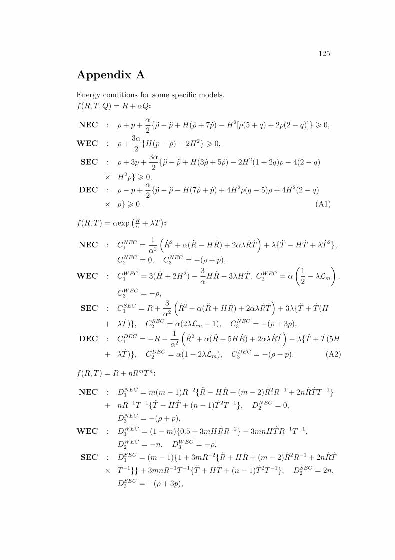
125

Appendix A

Energy conditions for some specific models.

f(R, T, Q) = R + αQ:

NEC : ρ + p +α

2ρ− p + H(ρ + 7p)−H2[ρ(5 + q) + 2p(2− q)] > 0,

WEC : ρ +3α

2H(p− ρ)− 2H2 > 0,

SEC : ρ + 3p +3α

2ρ− p + H(3ρ + 5p)− 2H2(1 + 2q)ρ− 4(2− q)

× H2p > 0,

DEC : ρ− p +α

2p− ρ−H(7ρ + p) + 4H2ρ(q − 5)ρ + 4H2(2− q)

× p > 0. (A1)

f(R, T ) = αexp(

Rα

+ λT):

NEC : CNEC1 =

1

α2

(R2 + α(R−HR) + 2αλRT

)+ λT −HT + λT 2,

CNEC2 = 0, CNEC

3 = −(ρ + p),

WEC : CWEC1 = 3(H + 2H2)− 3

αHR− 3λHT , CWEC

2 = α

(1

2− λLm

),

CWEC3 = −ρ,

SEC : CSEC1 = R +

3

α2

(R2 + α(R + HR) + 2αλRT

)+ 3λT + T (H

+ λT ), CSEC2 = α(2λLm − 1), CNEC

3 = −(ρ + 3p),

DEC : CDEC1 = −R− 1

α2

(R2 + α(R + 5HR) + 2αλRT

)− λT + T (5H

+ λT ), CDEC2 = α(1− 2λLm), CDEC

3 = −(ρ− p). (A2)

f(R, T ) = R + ηRmT n:

NEC : DNEC1 = m(m− 1)R−2R−HR + (m− 2)R2R−1 + 2nRTT−1

+ nR−1T−1T −HT + (n− 1)T 2T−1, DNEC2 = 0,

DNEC3 = −(ρ + p),

WEC : DWEC1 = (1−m)0.5 + 3mHRR−2 − 3mnHTR−1T−1,

DWEC2 = −n, DWEC

3 = −ρ,

SEC : DSEC1 = (m− 1)1 + 3mR−2R + HR + (m− 2)R2R−1 + 2nRT

× T−1+ 3mnR−1T−1T + HT + (n− 1)T 2T−1, DSEC2 = 2n,

DSEC3 = −(ρ + 3p),

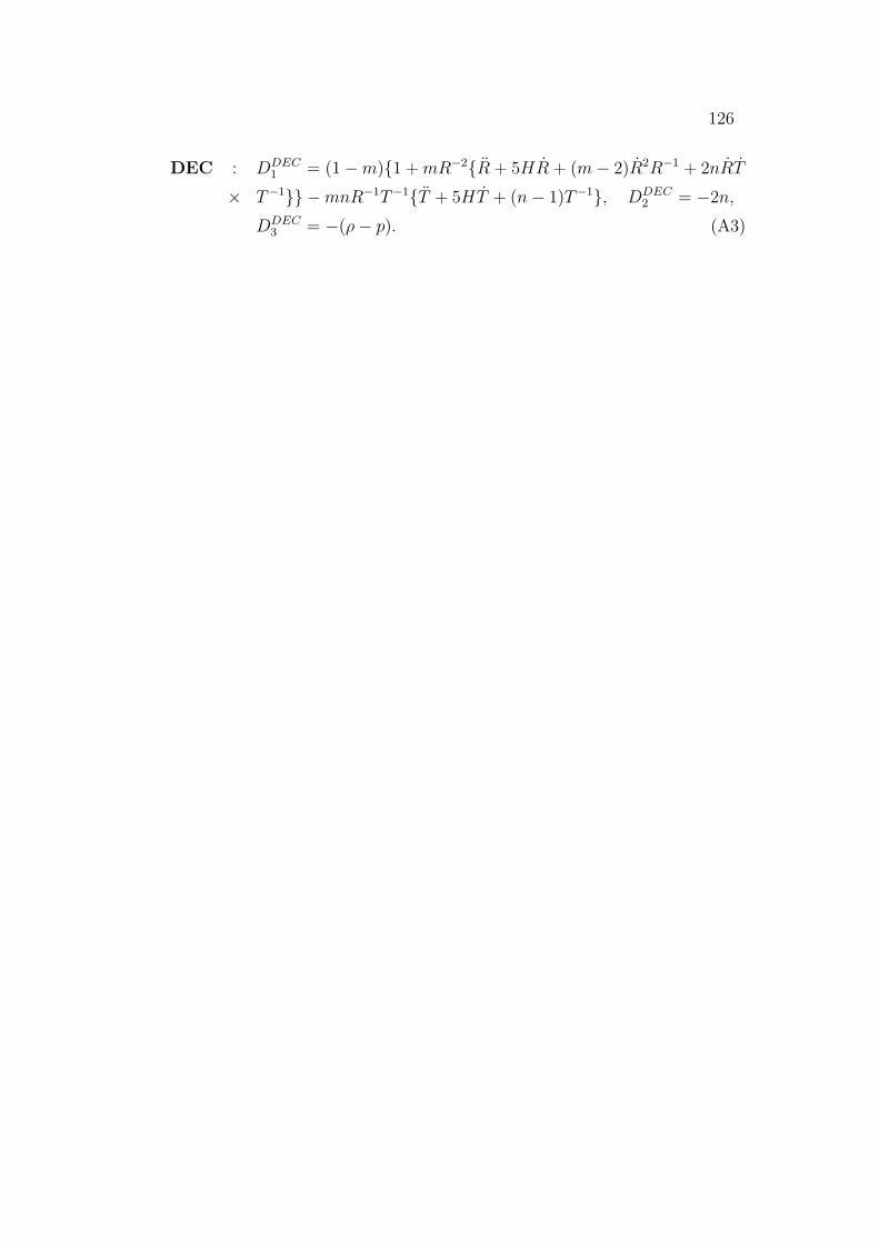
126

DEC : DDEC1 = (1−m)1 + mR−2R + 5HR + (m− 2)R2R−1 + 2nRT

× T−1 −mnR−1T−1T + 5HT + (n− 1)T−1, DDEC2 = −2n,

DDEC3 = −(ρ− p). (A3)

127

B: List of Publications

The contents of this thesis are based on the following research papers pub-

lished in journals of international repute. These papers are also attached

herewith.

1. Sharif, M. and Zubair, M.: Thermodynamics in f(R, T ) Theory of

Gravity, J. Cosmology Astroparticle Phys. 03(2012)028.

2. Sharif, M. and Zubair, M.: Study of Thermodynamic Laws in f(R, T, RµνTµν)

Gravity, J. Cosmology Astroparticle Phys. 11(2013)042.

3. Sharif, M. and Zubair, M.: Energy Conditions in f(R, T,RµνTµν)

Gravity, J. High Energy Phys. (to appear 2013).

4. Sharif, M. and Zubair, M.: Energy Conditions Constraints and Sta-

bility of Power Law Solutions in f(R, T ) Gravity, J. Phys. Soc. Jpn.

82(2013)014002.

5. Sharif, M. and Zubair, M.: Anisotropic Universe Models with Per-

fect Fluid and Scalar Field in f(R, T ) Gravity, J. Phys. Soc. Jpn.

81(2012)114005.

6. Sharif, M. and Zubair, M.: Study of Bianchi I Anisotropic Model in

f(R, T ) Gravity, Astrophys. Space Sci. 349(2014)457.

We have also published/submitted the following papers related to this the-

sis.

1. Sharif, M. and Zubair, M.: Evolution of the Universe in Inverse and

lnf(R) Gravity, Astrophys. Space Sci. 342(2012)511.

2. Sharif, M. and Zubair, M.: Cosmology of Holographic and New Age-

graphic f(R, T ) Models, J. Phys. Soc. Jpn. 82(2013)064001.

3. Sharif, M. and Zubair, M.: Analysis of f(R) Theory Corresponding

to NADE and NHDE, Adv. High Energy Phys. 2013(2013)790967.

4. Sharif, M. and Zubair, M.: Thermodynamic Behavior of Particular

f(R, T ) Gravity Models, J. Exp. Theor. Phys. 117(2013)248.

5. Sharif, M. and Zubair, M.: Reconstruction and Stability of f(R, T )

Gravity with Ricci and Modified Ricci Dark Energy, Astrophys. Space

Sci. 349(2014)529.

128

6. Sharif, M. and Zubair, M.: Thermodynamics in Modified Gravity with

Curvature Matter Coupling, Adv. High Energy Phys. 2013(2013)947898.

7. Sharif, M. and Zubair, M.: Cosmological Reconstruction and Stability

in f(R, T ) Gravity Gen. Relativ. Grav. 46(2014)1723.

8. Sharif, M. and Zubair, M.: Cosmological Evolution of Pilgrim Dark

Energy, Astrophys. Space Sci. DOI 10.1007/s10509-014-1889-8.

9. Sharif, M. and Zubair, M.: Reconstructing f(R) Theory from Pilgrim

Dark Energy, (Submitted).