C:/Users/Ana-Maria/OneDrive/paper2/Paper2 10 Jan 2015 and Information...School, London, 4-5 September 2014) in particular Neil R. Ericsson, Sir David Hendry, ... JEL classiﬁcation

Electronic copy available at: http://ssrn.com/abstract=2759360

Jumps and Information Asymmetry in the US

Treasury Market ∗

Ana-Maria H. Dumitru †

Giovanni Urga ‡

April 4, 2016

Abstract

This paper analyses the informational role of the trading activitywhen jumps occur in the US Treasury market. As jumps mark thearrival of new information to the market, we explore the contributionof jumps in reducing the informational asymmetry. We identify jumpsusing a combination of jump detection techniques. For all maturities,the trading activity is more informative in the proximity of jumps.For the 2- and 5-year maturities, there is a lower level of informationasymmetry before the jump, followed by a high level during the jumpwindow and up to 20 minutes after the jump occurs. Thus, the incor-poration of new information in prices is not instantaneous but severaltransactions are needed for the market to completely acknowledge thenew information. Finally, we propose the use of the estimated in-tegrated volatility as an exogenous predictor of jump occurrence inaddition to announcement surprises.

Keywords: Jumps, Nonparametric Tests, High Frequency Data, US

Treasury Market, Macroeconomic News, Information Asymmetry

JEL classification numbers: G12, G14, C01, C51

∗We wish to thank participants in the 15th OxMetrics User Conference (Cass BusinessSchool, London, 4-5 September 2014) in particular Neil R. Ericsson, Sir David Hendry,Sebastien Laurent, Bent Nielsen and Robert Yaffee for very insightful suggestions anduseful comments. The usual disclaimer applies.

†School of Economics, University of Surrey (UK). E-mail: [email protected]‡Cass Business School, City University London (UK) and Bergamo University (Italy).

E-mail: [email protected]

1

Electronic copy available at: http://ssrn.com/abstract=2759360

Jumps and Information Asymmetry in the US TreasuryMarket

Abstract. This paper analyses the informational role of the trading

activity when jumps occur in the US Treasury market. As jumps mark

the arrival of new information to the market, we explore the contribution of

jumps in reducing the informational asymmetry. We identify jumps using

a combination of jump detection techniques. For all maturities, the trading

activity is more informative in the proximity of jumps. For the 2- and 5-

year maturities, there is a lower level of information asymmetry before the

jump, followed by a high level during the jump window and up to 20 minutes

after the jump occurs. Thus, the incorporation of new information in prices

is not instantaneous but several transactions are needed for the market to

completely acknowledge the new information. Finally, we propose the use

of the estimated integrated volatility as an exogenous predictor of jump

occurrence in addition to announcement surprises.

Keywords: Jumps, Nonparametric Tests, High Frequency Data, US

Treasury Market, Macroeconomic News, Information Asymmetry

JEL classification numbers: G12, G14, C01, C51.

1

1 Introduction

Jumps can be defined as big and unexpected changes in the prices of

financial securities. The unanticipative nature of jumps stems from the fact

that they are informational events, i.e. the result of new information reaching

the market. Once this new information arrives to the market and the jump

occurs, information is homogeneously distributed to all market participants.

If before the jump there are agents with some degree of private information,

after the jump, everyone should have the same information. Thus, jumps

should reduce the degree of informational asymmetry in the markets.

The main objective of this present paper is to investigate the role of

jumps, as informational events, in dissipating informational asymmetry in

the US Treasury bond market. We identify jumps in bond prices using high

frequency data and combinations of nonparametric jump detection proce-

dures. Then, we measure the informational asymmetry in the proximity of

jumps, modifying the approach proposed in Green (2004). We consider var-

ious time windows before, at the time and after a jump takes place, as well

as in situations when no jumps occur. For the 2- and 5-year maturities, we

find that information asymmetry increases dramatically in the time window

when the jump occurs, and then stays relatively high for up to 20 minutes

after the jump has occurred. Moreover, information asymmetry reaches a

minimum immediately before the jump. Given that most of the jumps take

place as a result of macroeconomic announcements, this finding is consistent

with a low degree of information leakage before announcements. On the con-

trary, for the 10-year bond, there is evidence of higher levels of informational

asymmetry before jumps occur. This is very likely due to the higher degree

of uncertainty attached to bonds with longer maturities.

Our analysis builds upon Green (2004) who considers the release of

macroeconomic news as informational events. Indeed, in the US Treasury

market, the main source of information resides in macroeconomic news an-

nouncements (Fleming and Remolona, 1997; Balduzzi et al., 2001; Altavilla

et al., 2014). Moreover, in Section 2.2, we show that the vast majority

2

of jumps occur on days with macroeconomic news announcements. At the

same time, we show that only a small proportion of announcements (less than

13%) leads to jumps in prices and is thus relevant. In this paper, we propose

”jumps occurrence” as a natural way to discriminate between relevant and

irrelevant information: information is relevant if it leads to jumps in prices.

In addition, this paper brings several novel contributions to the recent

empirical literature on jump identification and determination, previously de-

veloped by Jiang et al. (2011), Lahaye et al. (2011), Boudt and Petitjean

(2014), Dungey et al. (2009) and Gilder et al. (2014). First, based on Du-

mitru and Urga (2012), we use a combination of testing procedures and

sampling frequencies to identify jumps in prices, the combination of tests be-

ing more robust than the use of the single procedure as applied in the above

mentioned papers. Second, we find that in the US Treasury market jumps

mainly occur as a result of macroeconomic news releases. Third, we show

that due to the simultaneity of jumps and news announcements, jumps are

almost always preceded by a significant liquidity withdrawal. Thus, while

previous research considers liquidity shocks as an important determinant of

the probability of jump occurrence, we argue that liquidity shocks and jumps

are endogenously jointly determined. As a consequence, we show that a ma-

jor cause of jump occurrence in the US Treasury market is still the release of

macroeconomic news. Finally, we further complement the literature on deter-

minants of jumps by proposing the use of the estimated integrated volatility

as an additional exogenous predictor of jump occurrence.

The paper is structured in the following way. Section 2 describes the

data, the interdealer market for the US Treasury bonds, the jump detection

procedures and the empirical results on jump detection. Section 3 reports

and discusses the bulk of our findings on the informational role of the order

flow when jumps occur. Section 4 concludes.

3

2 Preliminary analysis

2.1 Data and market description

Our analysis is based on high frequency data for four US Treasury bonds,

namely the 2-, 5-, 10- and 30-year bonds. The data was provided by Bro-

kerTec, an interdealer electronic trading platform and is made up of trade

records, quotations and order cancellations, as well as a work-up part. Due to

the complexity and scarcity of the data set, we include a short but insightful

description of the market and the data.

The interdealer brokerage market The secondary market for US Trea-

sury bonds is an interdealer over-the -counter market, where, as shown in

Fleming and Mizrach (2009) and Fleming (1997), there are 22-23 hours of

trading activity per day, with most of it being placed during New-York hours,

that is between 7:30 am and 5:00 pm. There are some trading peaks between

10:00 and 10:30 am and between 14:30 and 15:00.

The largest part of the transactions in the interdealer market for the US

Treasury bonds takes place through two large interdealer brokerage firms,

ICAP PLC with about 60% of market share and Cantor Fitzgerald with 28%

(Mizrach and Neely, 2006). Before 2000, both the actors on the marketplace

provided voice-assisted brokerage services. All the market data from ICAP

was collected in the GovPX database and was customarily used for the studies

concerning the US Treasury bonds. However, as noted by Mizrach and Neely

(2006), Boni and Leach (2004), Fleming (2003) and Barclay et al. (2006), with

the foundation of electronic trading platforms, most of the trading with US

Treasury bonds migrated from the voice-assisted to the electronic platforms.

Thus, as shown in Barclay et al. (2006), e-Speed, the electronic platform of

Cantor Fitzgerald was inaugurated in March 1999, while its main competitor,

BrokerTec, was set up in June 2000 and was purchased by ICAP in 2003.

These electronic trading platforms are characterized by lower transaction

costs and by a higher level of liquidity, also due to the fact that electronic

4

systems match opposite orders automatically, making the whole trading pro-

cess more fluid. The voice-assisted platforms remain though important for

their use for more “customized”, complex transactions that require human

intermediaries to perform negotiations between parties. Mizrach and Neely

(2006) show that after the introduction of the electronic trading platforms,

the average trading volume almost tripled from $200 billion in 1999 to $ 575

billion in 2005 .

Market characteristics The interdealer market is an expandable limit

order one, where transactions typically pass through three different phases

(Boni and Leach, 2004, see). Traders post limit orders, that can be auto-

matically matched by the electronic system. They can also respond to an

already existing order (becoming “aggressive”). However, as noted by Boni

and Leach (2004), there is an incentive on the market to provide liquidity

through limit orders, as commissions are paid only for responding orders.

The next phase of a transaction is the so-called “work-up” process. This

type of market provides the traders with the right of refusal to trade addi-

tional quantities, provided that the other party desires this. Thus, traders

usually enter limit orders in order to find counter-parties and then increase

quantities during the work-up process. Moreover, there is the possibility to

post “iceberg” orders, that have hidden quantities.

Once the parties agree on quantities, the trades are perfected and they

appear in the Trade section. Boni and Leach (2004) show that the right

and not the obligation to further increase traded quantities reduces the costs

associated with information leakage and stale limit orders, unlike the usual

limit order markets, where large orders might cause free-riding on the signal.

Fleming and Mizrach (2009), use BrokerTec data to reveal that liquidity

is greater than the one reported by studies using data from voice-assisted

brokerage platforms. Moreover, the iceberg orders are sparse and are mostly

used during volatile periods.

5

Dataset The data contains intraday observations covering the order book,

with both order submissions and cancellations, the trade section and the

work-up process for the 2-, 5-, 10- and 30-year bonds and covering a period

between January 2003 and March 2004. The choice of the period is related to

its relative calmness in comparison to other intervals during the last decade.

All nonparamentric tests for jumps identify excessive returns by comparison

to a local volatility measure. If volatility is very high, as during financial

crises, the tests are not able to pick up jumps anymore. While the first three

bonds are very liquid, for the 30-year one the competitor brokerage platform,

E-Speed, owns a bigger market share.

Prices are reported in 256th of a point and are maintained under this

form throughout the analysis, as they do not influence the results, given that

we work with log-returns.

For each trading day, we keep in our sample just the data comprised

between 7:30 a.m. EST and 5:00 p.m. EST, when trading is more active.

Sampling is done every 5 and 15 minutes. Based on the information in

the order book , we compute mid-quotes, spread and depth of the market at

the best bid and ask quotes. We rely on information in the trade section to

compute orderflow and trade volumes.

2.2 Jump detection

During the last decade, high frequency econometrics has seen several

contributions developing tests for jumps in the prices of financial assets (see

Barndorff-Nielsen and Shephard, 2006; Andersen et al., 2007; Lee and Myk-

land, 2008; Jiang and Oomen, 2008; Podolskij and Ziggel, 2010).

Dumitru and Urga (2012) show that the combination of detection proce-

dures and/or sampling frequencies improve the results of jumps tests when

prices are contaminated with microstructure noise. More precisely, unions

and intersections of the results of various testing procedures applied for differ-

ent sampling frequencies lead to improvements in the power of tests, without

impending on the size.

6

In this paper, we simultaneously rely on the results of the following jump

identification procedures: 1. the Barndorff-Nielsen and Shephard (2006)

applied on 5 minutes data (denoted BNS5); 2. the Barndorff-Nielsen and

Shephard (2006) applied on 15 minutes data (denoted BNS15); 3. the An-

dersen et al. (2007)-Lee and Mykland (2008) test applied on 15 minutes data

(denoted ABDLM15). To decide whether jumps occur at a certain day, we

consider as final test for jumps the following combination through unions of

intersections of the above tests:

(ABDLM15 ∩BNS5) ∪ (ABDLM15 ∩ BNS15)

Thus, the final days with jumps are the ones identified with the Lee and

Mykland (2008)- Andersen et al. (2007) test, if they were also detected by the

Barndorff-Nielsen and Shephard (2006) procedure on either 5 or 15 minutes

data.

Once a day with jump is identified as above, we rely on the results of

the ABDLM15 for that day to identify the time of the jump. As shown

below, the Andersen et al. (2007)-Lee and Mykland (2008) test, based on

standardized intraday returns, offers information not only on the day of the

jump, but also on the timing of the jump or jumps in that day, up to the

length of the sampling interval (15 minutes here). Moreover, the size of the

standardized return corresponding to the time of the jump gives us the jump

size. If more than one jump is detected within one day, all of them are taken

into consideration.

To further control for the impact of microstructure noise, the realized

bipower variation over 5 minutes data is based on staggered returns (An-

dersen et al., 2007). We rely on 99% critical values for all tests applied

here. Below, we report a short description of the jump detection procedures

implemented.

7

2.2.1 Jump tests

Barndorff-Nielsen and Shephard (2006) test This procedure tests the

null hypothesis of continuity of the sample path during a trading day. It relies

on comparing a robust to jumps volatility estimator, the realized bipower

variation (BVt), with a non-robust to jumps estimator, the realized variance

(RVt). Based on the results of the simulation in Huang and Tauchen (2005),

we employ the ratio test statistic:

1− BVt

RVt√0.61 δ max

(1, TQt

BV 2t

)L→ N (0, 1) (1)

where t is the end of the time interval of interest, [0, t] , and TPt denotes the

realized tripower variation. To define RVt, BVt and TPt, the time interval

[0, t] is split into n equal subintervals of length δ. The j-th intraday return

rj on day t is rj = pt−1+jδ − pt−1+(j−1)δ, where pt−1+jδ is the j-th logarithmic

price observed on day t, j = 1 . . . n. We then have:

RVt =n∑

j=1

r2j (2)

BVt = 1.57n∑

j=2

|rjrj−1| (3)

TPt = n 1.74

(n

n− 2

) n∑

j=3

|rj−2|4/3|rj−1|4/3|rj|4/3 (4)

Lee and Mykland (2008)-Andersen et al. (2007) test Lee and Myk-

land (2007) and Andersen et al. (2007) concurrently develop tests for jumps

based on the standardization of the intraday returns by the square root of

the realized bipower variation. While Andersen et al. (2007) use observations

of the whole trading day to compute BVt, Lee and Mykland (2008) estimate

it on a local window that precedes the time when the test is performed. Both

tests have the null hypothesis of continuity of the sample path at a certain

8

time, tj. This allows users to identify both the exact time of a jump as

well as the number of jumps within a trading day. The following statistic is

considered:

zj =|rj|√BVt/n

L→ N (0, 1), j = 1 . . . n, (5)

Both papers point out that the usual normal critical values (95% and

99% percentiles) are too permissive. To address this issue, Andersen et al.

(2007) treat it as a multpiple testing problem and use the Sidak correction

leading to a test size β = 1 − (1 − α)δ, where α is the daily size. Lee and

Mykland (2008) propose using the distribution of the maximum of the above

statistic over the trading day. The new properly standardized statistic will

display an extreme value distribution (Gumbel distribution):

max zj − Cn

Sn

→ ξ, P(ξ) = exp(−e−x), ∀j = 1, 2, . . . , n (6)

where Cn = (2 logn)1/2

µ1

− log π+log (log n)

2µ1(2 logn)1/2 and Sn = 1

µ1(2 logn)1/2 . In this paper, we

rely on critical values as in Lee and Mykland (2008).

Boudt et al. (2011) notice that the volatility estimator used to standard-

ize the returns in (5) changes very slowly, while intraday volatility tends to

cluster and peak during the same time intervals within a trading day. They

propose parametric and nonparametric estimators of the periodicity factor

that are robust to the presence of jumps. Here, we only describe the non-

parametric approach that we use to correct the test statistic in (5). Let the

intraday returns be described by the following discrete model:

yj = fjsjuj + aj, j = 1 . . . n, (7)

where sj is the average bipower variation, estimated on a local window

around j, fj = σj/sj, the periodicity factor, with σj the spot volatility,

uj ∼ i.i.d.N (0, 1).

The periodicity factor is estimated as follows. First, we standardize all

intraday returns by the squared root of the properly scaled realized bipower

9

variations estimated on a local window around j. Let r(1),j ≤ r(2),j ≤ . . . ≤r(nj),j be the ordered standardized returns in a window around time j. Sec-

ond, we compute Rousseeuw and Leroy (1988)’ “shortest half scale estimator”

on these returns.

ShortHj = 0.741min{r(hj),j − r(1),j , . . . , r(nj),j − r(nj−hj+1),j}, (8)

where hj = [nj/2] + 1. This estimator can be subsequently standardized to

fShortHj =

ShortHj

1

n

√ShortH2

j

.

The final periodicity estimator is the standardized Weighted Standard

Deviation (WSD):

fWSDj =

WSDj

1n

√WSD2

j

, (9)

with WSDj =

√1.081

∑njl=1

wl,jr2

l,j∑njl=1

wl,j

, where the weights wl,j are given by:

wl,j =

1, if (rl,j

fShortHj

)2 ≤ 6.635

0, otherwise

2.2.2 Detected jumps

We find that the 2-year bonds jump in 14.5% of the days, the 5-year in

10.6%, the 10-year in 9.6% and finally the 30-year in 17.91% of the days. As

expected, if we do not consider the result for the 30-year bond, we observe

a decrease in the proportion of identified jumps with the increase in the

maturity. The 30-year bond is highly illiquid during the period we considered

in our sample and thus we expect the high proportion of detected jumps is

spuriously generated.

Table 1 reports some descriptive statistics on the estimated jump sizes

for all the maturities, while Table 2 reports the same indicators but for jump

sizes that were previously standardized by a local volatility estimator. The

biggest size is encountered in the case of the 30-year bond, but we suspect

10

this finding is due to liquidity issues, just as the high proportion of jumps

identified for this maturity. If we ignore this maturity, when we look at all

central tendency parameters in Table 1, we observe that the 10-year bond

displays the highest jump size, followed by the 5-year and the 2-year. It seems

that the latter jumps more frequently, but less abruptly than the other bonds.

However, if we standardize these jumps by robust to jumps local volatility

estimators, we observe (see Table 2) that the previous hierarchy disappears,

indicating that the shorter maturity bonds are less volatile than the others.

SizeMean Median Mode Std

Y2 0.081% 0.063% 0.023% 0.052%Y5 1.787% 0.181% 0.000% 10.394%Y10 1.795% 0.292% 0.000% 9.814%Y30 2.127% 0.474% 0.211% 9.639%

Table 1: Summary statistics for the estimated jump size for the 2-, 5-, 10-and 30-year US Treasury bonds

Standardized SizeMean Median Mode Std

Y2 31.15 23.57 16 19.39Y5 28.38 22.25 16.07 15.67Y10 28.36 24.19 15.91 13.24Y30 30.19 21.8 16.04 30.15

Table 2: Summary statistics for the standardized jump size for the 2-, 5-, 10-and 30-year US Treasury bonds

Table 3 reports the number of common jumps between maturities, when

taken two by two. We observe a clear prevalence of common jumps at the

shorter end of the term structure. Thus, we have the largest number of

co-jumps for combinations of the 2-year maturity with the other bonds.

The main conclusion is that the shorter maturity bonds jump more fre-

quently than the others. This suggests that they react to a larger proportion

of macroeconomic announcements than the others, meaning that they are

more sensitive to events occurring in the economic environment. The other

11

Y2 Y5 Y10 Y30Y2 44 28 24 23Y5 32 21 17Y10 29 17Y30 53

Table 3: Number of jumps (diagonal elements) and co-jumps (off-diagonalelements) for the 2-, 5-, 10- and 30-year US Treasury bonds

Y2 Y5 Y10 Y30Match 94 92.16% 79 100.00% 60 93.75% 72 83.72%

No match 8 7.84% 4 6.25% 14 16.28%Total 102 100.00% 79 100.00% 64 100.00% 86 100.00%

Table 4: Number and percentages of jumps matched with macroeconomicannouncements

bonds are less sensitive, displaying a lower probability of jump occurrence,

but, given the long maturity, they transpose the environment uncertainty to

larger moves in the prices.

2.2.3 Determinants of jumps

For each maturity and for each jump, we check whether on the day and

around the time of the jump there were any macroeconomic announcements.

Data on announcements is taken from Yahoo! Finance, which reports some

of the data provided by Briefing.com. A complete list of all relevant an-

nouncements is included in Appendix A.

For each maturity, we compute the number and percentage of jumps to

which macroeconomic announcements can be associated, as well as jumps

which cannot be matched with any news releases. Results are summarized in

Table 4. For the 2-, 5- and 10-year bonds, more than 90% of the jumps can be

associated with the release of public information to the market. For the 30-

year bond, this percentage equals only 83.73%, which we believe is due to the

spurious detection of jumps that cannot be matched with announcements.

Once we identified all news releases that can impact on bond prices, we

12

Y2 Y5 Y10 Y30Big surprise 64 64 64 64

Big surprise & no jump 57 89.06% 57 89.06% 56 87.50% 64 100.00%

Table 5: Number of big announcement surprises and number and percentagesof those not associated with any jump (big surprises are defined as larger thanthe 95% quantile of the normal distribution).

compute the absolute value of the announcement surprise, provided data on

this is available. We standardize each surprise by the standard deviation of all

surprises available for the same announcement during the period considered

in our sample. We select all standardized surprises larger than the 95%

quantile of the normal distribution and examine whether jumps took place

on the corresponding days and times. Surprisingly, for all maturities, we

identify a very low percentage of ‘big’ surprises associated with jumps. The

results are summarized in Table 5.

While more than 90% of the jumps are generated by announcements, it

seems that approximately 90% of the announcements do not cause jumps.

These results can be explained by several factors. First, given our sample

of just 15 months, for each type of news release, we have just a few sur-

prises. Thus, the standard deviation of each type of surprise is computed

on a very small sample and thus, subject to biases. Second, there are cer-

tain announcements that are more important than others and jumps can

occur even if surprises are not very big. Third, as suggested by Hess (2004),

the “timeliness” of the news releases might be important, as well. If sev-

eral announcements reveal similar information, the earlier ones should have

a greater impact on the prices.

The liquidity around jump times puzzle Previous research identifying

determinants of jumps in the prices of financial assets find that liquidity

shocks preceding jumps are very good predictors of jump occurrence (Jiang

et al., 2011; Boudt and Petitjean, 2014). Jiang et al. (2011), who use the same

data set as us but a slightly different sample, find that when liquidity shocks

13

and news surprises are jointly considered as determinants of jump occurrence,

news surprises tend to lose their significance. Our descriptive analysis above,

though, shows that in the US Treasury market, the vast majority of jumps

(over 90%) can be matched to macroeconomic announcements. The above

statements give rise to what we call here the “liquidity around jump times

puzzle”, which we explain below.

Macroeconomic announcements have long been documented to constitute

the main source of information concerning the fundamental value of govern-

ment bonds (Balduzzi et al., 2001; Andersen et al., 2003; Hess, 2004; Green,

2004; Dungey et al., 2009). Consequently, US Treasury bond prices were

shown to react to news releases. This abundant evidence in addition to our

own descriptive evidence in the previous paragraph prove beyond no doubt

that news releases are the main drive for jumps in bond prices. Moreover, we

show below that the simultaneity of jumps and macroeconomic announce-

ments can generate liquidity shocks preceding jumps.

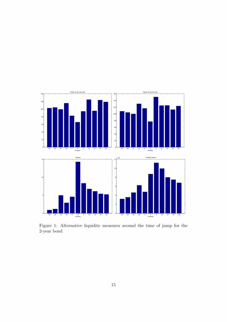
We measure several liquidity indicators on a window of -/+ 25 minutes

around the time of the jump and examine their behavior within this interval.

We consider the depth of the market at the best bid and ask quotes, the

spread and the trading volume. Figure 1 illustrates these different measures

for the 2-year bond. The corresponding figures for the other maturities are

comprised in Appendix B. As the depth indicators refer to the best bid and

ask quotes, they are both expressed in number of contracts.

Both the depth at the best ask quote and the one at the best bid quote

fall in the 5-10 minutes that precede the jump. Spread peaks within the 5

minutes interval before the occurrence of the jump, while the trade volume

falls in the 5-10 minutes before the jump and then experiences an abrupt

increase. Thus, all these liquidity measures show a severe withdrawal of

liquidity before the jump occurrence.

The observed liquidity withdrawal can be explained by the simultaneity

of most jumps with macroeconomic announcements. Before macroeconomic

announcements, market participants limit their trading activity waiting to

14

−25 −20 −15 −10 −5 0 5 10 15 20 250

20

40

60

80

100

120

140Depth on the ask side

minutes−25 −20 −15 −10 −5 0 5 10 15 20 25

0

20

40

60

80

100

120

140

160Depth on the bid side

minutes

−25 −20 −15 −10 −5 0 5 10 15 20 250

5

10

15Spread

minutes−25 −20 −15 −10 −5 0 5 10 15 20 25

0

2

4

6

8

10

12x 10

6 Trading volume

minutes

Figure 1: Alternative liquidity measures around the time of jump for the2-year bond

15

find out the content of the news release. As most jumps occur after news re-

leases, they will always be accompanied by the observed liquidity withdrawal.

This makes us believe that jumps and liquidity shocks before jumps are en-

dogenously determined, being both caused by the release of macroeconomic

information.

A simple regression model explaining the jump occurrence in the

US Treasury market. In order to quantify the impact of announcement

surprises on jumps, we estimate an extreme value (Gumbel) binary choice

model in which we consider as determinants of the probability of jump occur-

rence the announcement surprise and the square root of the bipower variation

estimate for the corresponding trading day, based on 5 minutes staggered re-

turns. The inclusion of the volatility estimator has two major rationales.

First, it is sensible to believe that if jumps occurred within one day, volatil-

ity increased as well. To avoid endogeneity issues, we consider here just the

volatility coming from the continuous part of the price process and not the

one including the jumps. Second, we believe that a volatility proxy might

capture other unknown factors that could contribute to the price dynamics

but which might be hard to identify and observe. In our analysis, we take

into consideration all the days in our sample, independent of whether news

were released or not on that day. The dependent variable is set to 1 if at

least one jump occurred on a certain day and to 0 otherwise.

Table 6 includes the estimation output for these binary choice regressions.

The choice of the extreme value distribution is based on the reported Akaike,

Schwartz and Hannan-Quinn information criteria.

We observe that the surprise is significant at a 1% significance level for the

2-, 5- and 10-year bonds and at a 5% significance level for the less liquid 30

-year bond. Our proxy for volatility is also found highly significant (1%) for

the 2-, 5- and 30-year bonds, while for the 10-year one we have significance

only at a 5% significance level. In the same table we report results for

the Hosmer-Lemeshow goodness-of-fit test for binary choice models, which

16

Coefficient p-value Goodness of fitY2 C -2.53 0.0000 H-L Statistic 5.74

Surprise 0.29 0.0021 Prob. Chi-Sq(8) 0.68Volatility (BV) 1881.19 0.0000

Y5 C -2.37 0.0000 H-L Statistic 4.36Surprise 0.40 0.0002 Prob. Chi-Sq(8) 0.82

Volatility (BV) 432.54 0.0002





Table 6: Results from regressing the probability of a jump on a constant (C),the announcement surprise and volatility, measured as the realized bipowervariation (BV)

compares values predicted by the model with the real values of the dependent

variable. Results in Table 6 suggest that differences between actual and

predicted values are not significant, indicating a good fit.

3 Informativeness of the order flow when

jumps occur

Jumps are unanticipated sized changes in prices. They are related to

fundamentals of financial assets and reflect new information coming to the

market. Because of their role in marking the incorporation of new informa-

tion in the price, one would expect a significant decrease in informational

asymmetry following jump occurrence. Thus, once information is released

and a jump takes place, the trading process should gradually become less

and less informative. The first objective of this section is to test the validity

17

of this intuitive hypothesis.

In the US Treasury market, new information is customarily related to the

release of macroeconomic news. Whenever the content of such news is unan-

ticipated by the market, we expect to observe a jump. The unanticipative

nature of new information when prices jump implies a low degree of infor-

mational asymmetry in the interval preceding the jump. This is congruent

with the absence of informational leakage before jumps occur. Testing the

validity of this hypothesis is the second objective of this section.

Our analysis follows the framework of Green (2004), who examines the

impact of trading on bond prices around news releases. The author finds a

very low degree of informational asymmetry before announcements, accom-

panied by a significant increase in the informational role of trading following

announcements. However, as observed in the previous section, while the ma-

jority of jumps in this market are caused by macroeconomic announcements,

not all announcements lead to jump occurrence. Jumps occur if and only if

information is relevant. For this very reason, it is worthwhile introducing into

analysis a new category of informational events: jumps themselves. This is

made possible by the recent advances in the econometrics of jump detection

based on high frequency data which followed Green (2004)’s seminal work.

Green (2004)’s analysis relies on data for the 5-year bond. Here, we use

data for the 2-, 5-, 10- and 30-year maturities. This gives us the opportunity

to explore whether the behaviour of various maturities in terms of informa-

tiveness of the order flow when jumps occur is similar or not. This constitutes

a third objective of this section.

The starting point of our analysis is Madhavan et al. (1997)’ model of

price formation (denoted as MRR):

pti − pti−1= (φ+ θ)xti − (φ+ ρθ)xti−1

+ eti , (10)

where ti are the times when trades take place, i = 1 . . . N , with N the total

number of trades, xti is the order flow at time ti, with xti = 1 if the transac-

tion is buyer initiated and xti = −1 if the initiator was the seller, φ captures

18

the compensation for providing liquidity, including all order processing costs,

but also the effects of dealer inventories, ρ is the autocorrelation in the order

flow, while θ measures the information asymmetry. The latter is the most

important parameter in our analysis and assesses the impact of the surprise

in the order flow (xti − ρxti−1) on price changes.

3.1 Models

In order to analyze how the parameters of the above model change in the

presence of jumps, we transform equation (10), by adding several dummies,

resulting in the following five models:

Model 1

pti − pti−1=(φJ + θJ)IJ,tixti − (φJ + ρθJ)IJ,tixti−1

+ (φNJ + θNJ)INJ,tixti−(φNJ + ρθNJ)INJ,tixti−1

+ eti ,

(11)

where the parameters are estimated separately for the days with jumps

(IJ,ti = 1) and for those without jumps (INJ,ti = 1).

Model 2

pti − pti−1=(φJ0 + θJ0)IJ,tiIJ0,tixti − (φJ0 + ρθJ0)IJ,tiIJ0,tixti−1

+ (φB + θB)IJ,tiIB,tixti−(φB + ρθB)IJ,tiIB,tixti−1

+ (φA + θA)IJ,tiIA,tixti − (φA + ρθA)IJ,tiIA,tixti−1+

(φNJ + θNJ)INJ,tixti − (φNJ + ρθNJ)INJ,tixti−1 + eti ,

(12)

where, for the days with jumps, we differentiate between the moment of the

jump, J0 and the periods before (B) and after (A) the jump.

19

Model 3


+

(φB5 + θB5)IJ,tiIB5,tixti − (φB5 + ρθB5)IJ,tiIB5,tixti−1+

(φA5 + θA5)IJ,tiIA5,tixti − (φA5 + ρθA5)IJ,tiIA5,tixti−1+

(φother + θother)Iother,tixti − (φother + ρθother)Iother,tixti−1+ eti

(13)

where, for the days with jumps we consider a window of -/+ 5 minutes around

the jump and estimate parameters at the jump time (J0), for the 5 minutes

that precede the jump (B5), for the 5 minutes after the jump (A5) and for

the rest of the data (other).

Model 4


+



(φother + θother)Iother,tixti − (φother + ρθother)Iother,tixti−1+ eti ,

(14)

just as model 3, but the window is of -/+ 10 minutes around the jump time.

Model 5


+



(φother + θother)Iother,tixti − (φother + ρθother)Iother,tixti−1+ eti ,

(15)

just as model 3, but the window is of -/+ 20 minutes around the jump time.

To estimate the above models, we use all the transaction data available.

Given that jumps are identified based on 5/15 minutes data, we cannot per-

20

fectly match the times of the jumps with the times of the trades. Thus, the

indicator function IJ0,ti selects a window of +/- 2 minutes around the jump

time. All the other indicator functions that select observations around the

times of the jumps are adapted accordingly. For instance, IB10,ti selects all

observations preceding a certain jump time with 12 to 2 minutes.

The Generalized Method of Moments is employed to estimate the co-

efficients of the above equations. We exemplify here only the estima-

tion of model 1, as the estimation for the others is very similar. Let

β = (α, ρ, φJ , θJ , φNJ , θNJ) be the vector of parameters to estimate for model

1, with α the intercept added to the model. In order to find the estimates

for the components of this vector, the following moment conditions are used:

E

xtixti−1− x2

tiρ

eti − α

(eti − α)IJ,tixti

(eti − α)IJ,tixti−1

(eti − α)INJ,tixti

(eti − α)INJ,tixti−1

= 0 (16)

The estimates are robust to ARCH-type heteroskedasticity.

3.2 Empirical results

Results for the 2-, 5- and 10-year bonds are summarized in Tables 7-9.

Results for the 30-year maturity may be affected by the low liquidity that

characterizes the data for this maturity. Consequently, for completeness we

report them only in the Appendix C, Table 11. The estimated coefficients

for this maturity behave, in terms of size, for all models, very similarly to

the estimates for the 2- and 5-year maturities. However, for the days with

jumps, coefficients are usually insignificant, probably due to the low number

of observations used to estimate them.

As already mentioned, the focus of our analysis are the θ parameters.

21

Model 1

Coefficient Std. Error t-Statistic p-valueα 0.0035 0.0012 2.94 0.0032

φJ 0.0310 0.0141 2.20 0.0275θJ 0.3759 0.0118 31.81 0.0000

φNJ 0.0456 0.0040 11.33 0.0000θNJ 0.3258 0.0036 90.58 0.0000

Model 2 Model 3

Coefficient Std. Error t-Statistic p-value Coefficient Std. Error t-Statistic p-valueα 0.0034 0.0012 2.90 0.0037 α 0.0034 0.0012 2.88 0.0039

φJ0 -0.8520 0.5397 -1.58 0.1144 φJ0 -0.8421 0.5381 -1.57 0.1176θJ0 1.3779 0.4303 3.20 0.0014 θJ0 1.5269 0.4259 3.59 0.0003φB 0.0653 0.0246 2.66 0.0079 φB5 0.1910 0.1397 1.37 0.1716θB 0.2858 0.0194 14.76 0.0000 θB5 0.3446 0.0605 5.70 0.0000φA 0.0316 0.0125 2.53 0.0112 φA5 -0.1346 0.1262 -1.07 0.2860θA 0.3595 0.0111 32.43 0.0000 θA5 0.6672 0.0944 7.07 0.0000

φNJ 0.0456 0.0040 11.33 0.0000 φother 0.0460 0.0038 12.19 0.0000θNJ 0.3258 0.0036 90.58 0.0000 θother 0.3292 0.0034 97.70 0.0000

Model 4 Model 5


φJ0 -0.8421 0.5381 -1.56 0.1176 φJ0 -0.8420 0.5403 -1.56 0.1192θJ0 1.5276 0.4259 3.59 0.0003 θJ0 1.4193 0.4316 3.29 0.0010

φB10 0.1536 0.0797 1.93 0.0541 φB20 0.1235 0.0618 2.00 0.0455θB10 0.2460 0.0476 5.16 0.0000 θB20 0.2660 0.0424 6.27 0.0000φA10 -0.0834 0.0770 -1.08 0.2789 φA20 -0.0559 0.0472 -1.18 0.2364θA10 0.5729 0.0614 9.33 0.0000 θA20 0.5064 0.0400 12.65 0.0000

φother 0.0465 0.0038 12.30 0.0000 φother 0.0473 0.0038 12.47 0.0000θother 0.3279 0.0034 97.58 0.0000 θother 0.3262 0.0034 96.68 0.0000

Table 7: Estimated coefficients, standard errors, t-statistics and p-values, respectively, for Models 1-5 for the 2-yearbond. For all models, the value of the correlation coefficient for the order flow is ρ = 0.6609

22

Model 1


φJ -0.1710 0.0216 -7.92 0.0000θJ 0.8575 0.0197 43.63 0.0000

φNJ -0.1767 0.0056 -31.29 0.0000θNJ 0.8454 0.0073 115.18 0.0000

Model 2 Model 3


φJ0 -1.6179 0.9121 -1.77 0.0761 φJ0 -1.6712 0.9138 -1.83 0.0674θJ0 2.9582 0.8663 3.41 0.0006 θJ0 3.2768 0.8655 3.79 0.0002φB -0.1746 0.0421 -4.15 0.0000 φB5 -0.2157 0.1475 -1.46 0.1435θB 0.7612 0.0336 22.64 0.0000 θB5 0.7726 0.1386 5.57 0.0000φA -0.1303 0.0208 -6.26 0.0000 φA5 -0.0168 0.2863 -0.06 0.9533θA 0.7883 0.0179 44.14 0.0000 θA5 1.1441 0.1336 8.57 0.0000

φNJ -0.1767 0.0056 -31.29 0.0000 φother -0.1731 0.0053 -32.63 0.0000θNJ 0.8454 0.0073 115.18 0.0000 θother 0.8410 0.0067 125.50 0.0000

Model 4 Model 5


φJ0 -1.6698 0.9138 -1.83 0.0676 φJ0 -1.6072 0.9128 -1.76 0.0783θJ0 3.2773 0.8655 3.79 0.0002 θJ0 3.0325 0.8731 3.47 0.0005

φB10 -0.2633 0.1051 -2.51 0.0122 φB20 -0.3145 0.1502 -2.09 0.0363θB10 0.7290 0.1034 7.05 0.0000 θB20 0.8049 0.1085 7.42 0.0000φA10 -0.1813 0.1683 -1.08 0.2813 φA20 -0.1205 0.1018 -1.18 0.2366θA10 0.9441 0.0836 11.29 0.0000 θA20 0.8408 0.0639 13.16 0.0000

φother -0.1721 0.0053 -32.48 0.0000 φother -0.1718 0.0053 -32.37 0.0000θother 0.8404 0.0067 125.03 0.0000 θother 0.8397 0.0068 124.32 0.0000


23

Model 1


φJ -0.1040 0.0430 -2.42 0.0155θJ 1.3216 0.0419 31.55 0.0000

φNJ -0.2017 0.0119 -16.93 0.0000θNJ 1.3647 0.0104 130.61 0.0000

Model 2 Model 3


φJ0 -0.8359 1.7737 -0.47 0.6374 φJ0 -0.9096 1.7708 -0.51 0.6075θJ0 0.0004 1.5499 0.00 0.9998 θJ0 0.5169 1.5494 0.33 0.7387φB -0.0302 0.0803 -0.38 0.7073 φB5 0.5159 1.2391 0.42 0.6772θB 1.0373 0.0964 10.76 0.0000 θB5 2.3117 0.9639 2.40 0.0165φA -0.0882 0.0418 -2.11 0.0347 φA5 0.1530 0.2963 0.52 0.6056θA 1.2630 0.0410 30.82 0.0000 θA5 1.7152 0.2743 6.25 0.0000


Model 4 Model 5


φJ0 -0.9097 1.7711 -0.51 0.6075 φJ0 -0.8725 1.7801 -0.49 0.6240θJ0 0.5198 1.5496 0.34 0.7373 θJ0 -0.0529 1.5444 -0.03 0.9727

φB10 0.2787 0.4956 0.56 0.5739 φB20 -0.3082 0.4060 -0.76 0.4478θB10 1.5666 0.6596 2.37 0.0176 θB20 1.9321 0.5167 3.74 0.0002φA10 -0.0195 0.2731 -0.07 0.9430 φA20 0.1541 0.1648 0.94 0.3498θA10 1.5090 0.2892 5.22 0.0000 θA20 1.3630 0.1551 8.79 0.0000


Table 9: Estimated coefficients, standard errors, t-statistics and p-values, respectively. for Models 1-5 for the 10-yearbond. For all models, the value of the correlation coefficient for the order flow is ρ = 0.6725

24

Below, we discuss the values of the θs for Model 1 and Model 2 separately

and then for Models 3-5 jointly. We complete this section with some brief

discussions of the estimates of the φs and ρs for all models considered.

Model 1. In general, if we look at results for Model 1 for all maturities,

we observe that the estimates of θ tend to increase with maturity. Thus, for

the 2-year bond, θ takes the value .38 for days with jumps and .33 for days

without jumps. For the 5-year bond, the same estimated parameters are

about .85 and .84, while for the 10-year bond the values are 1.32 and 1.36.

This increase in the coefficients with the maturity is due to the fact that

price changes tend to be higher for longer maturities, which is also consistent

with the fact that jump sizes are bigger for higher maturities.

The results for Model 1 in Tables 7 - 9 indicate that the estimates of θ do

not vary much between days with jumps and days without jumps. For the 2-

and 5-year maturities, estimates for θJ are bigger than those for θNJ , while

for the 10-year maturity, the results are reversed. The close values of θs for

jump days and days without jumps are not surprising. As these coefficients

are measured for data within a whole day, they confer an average value for

information asymmetry. This suggests that the order flow informativeness

is transitory. Results for the more complex models below will confirm this

fact, showing that trading can become informative for a certain period in the

proximity of a jump, but then this effect dissipates.

Model 2. In this model, we separately estimate coefficients for the ‘jump

window’, which is -/+ 2 minutes around the jump time. Moreover, we split

the days with jumps in intervals that precede jumps and periods that follow

them. Evidence for all maturities indicate that θ takes higher values after

the jump than before. For instance, for the 2-year maturity, we have θB =

0.29 and θA = 0.36. Moreover, for the 2- and 5-year bonds, information

asymmetry dramatically increases when jumps occur (θJ0 = 1.38 for the

2-year bond and θJ0 = 2.96 for the 5-year bond).

The low levels of θB are consistent with the absence of informational

25

leakage before a jump occurs. After a jump occurs, for the first two maturi-

ties,the degree of informativeness of the orderflow jumps also to a very high

level and then decreases again. This high levels can be explained by the fact

that after the jump, the trading activity significantly intensifies and thus,

also becomes more informative. θA is higher for all maturities than θB and

has relatively close levels to θNJ . This indicates that after a jump, θ returns

to what are considered to be “normal” values.

For the 10-year maturity, the coefficient that captures information asym-

metry for the ‘jump window’ is not significant at 1% or 5% significance levels

(see Table 9 on page 24). We believe this might be because the ‘jump win-

dow’ (-/+ 2 minutes around the jump time) we used was too narrow. Con-

sequently, we extend this window to -/+ 5 minutes around the jump time

and widen all the other windows accordingly. Estimates of all the models for

the 10-year maturity are reported in Table 12 in Appendix C. If we look at

results for Model 2, we observe that the estimate of θJ0 increases to 1.14 and

is significant at a 5% significance level, but is still lower than θA and θNJ .

Models 3-5. In these models, we narrow our analysis to those intervals of

time that are very close to the time of the jump. We maintain the ‘jump

window’ of -/+ 2 minutes around the identified time of the jump and build

windows of 5 (Model 3), 10 (Model 4) and 20 (Model 5) minutes before and

after the jump.

The 2- and 5-year maturities exhibit a similar behavior. θs are very high

at the jump time, they are quite low before the jump and remain at higher

levels after the jump. For the 2-year bond, for instance, θJ0 = 1.52 for all

the three models, θB is quite low, varying from 0.12 for Model 5 to 0.34 for

Model 3, while θA, with values between 0.51 and 0.66 is considerably higher

than θother and θB. A similar scaling between θB and θA is maintained for

the 30-year bond, as shown in Appendix C, Table 11.

The estimator of θB has the lowest value of all the θs, reflecting again

the no leakage hypothesis. In addition, as shown in the previous section, the

26

trading activity decreases before the jump and there is a significant liquidity

withdrawal. Thus, it is possible that in the immediate window preceding the

jump, the trading activity is not very informative because there is not much

trading going on. In fact, as we move from Model 3 to 5 and increase the

window before the jump, θB also increases, as more trading is likely to occur

in a wider time window.

θA is higher than the values of θs before the jump and for all other ob-

servations. After the jump, trading intensifies for a certain time interval and

then moves back to normal levels. This is reflected by the fact that θA is

higher for the 5 minute after jump window (Model 1) and lowest for the 20

minute window (Model 3).

For the 10-year bond, results are contradictory to the ones for the first

two maturities and to results obtained for Model 2 for the same maturity.

θJ0 is again insignificant, while θA is lower than θB for all models. We offer

here two sets of explanations for the inconsistency of results for this maturity

with results for shorter maturities. A combination of the two could also be

possible.

1. These results are sample dependent and could potentially change if

the analysis were repeated on a much larger sample. The limitations

in terms of sample size for this analysis do not regard the number of

transactions, but the number of identified jumps. For the 10-year bond,

we only observe 29 jumps, a lower number than for shorter maturities.

Moreover, jump identification is a statistical procedure, subject to er-

ror. Given the low number of jumps, if the right timing of some jumps

was not identified correctly, it could potentially affect the estimates for

all coefficients of interest, θJ0, θA and θB.

2. Longer maturity bonds are well known to carry more uncertainty and

to be less tied to macroenomic policy. The high informational asymme-

try found before a jump takes place could potentially reflect this higher

degree of uncertainty. Market participants do not know whether the

27

following news release would be relevant or not and thus, every trade

occurring is perceived as informative. At the same time, once informa-

tion arrives to the market, its content needs to be of extreme relevance

in order to impact prices of longer maturity bonds. Thus, a very lim-

ited number of the very dense macroeconomic news releases will impact

the longer maturity bonds. Due to this limited responsiveness of longer

maturities to news releases, there is a mutual agreement in the market

about the price level after the correction induced by the jump. Thus,

even if trading intensifies after the jump, the price changes induced by

trades are not substantial.

For all maturities, θ increases dramatically in a window after or before the

jump. This suggests that the incorporation of new information in prices is

not instantaneous. It takes several transactions for the market to completely

acknowledge the new information. The length of this process of incorpo-

rating new information into the transaction prices depends on the depth of

the order book, which undergoes several changes once new information is

released. More precisely, following the release of information, market par-

ticipants re-adjust their orders, which will then be executed in the order of

submission. The transaction prices will experience several “re-adjustment

jumps” to acknowledge the new state of the world. Thus, one jump in the ef-

ficient, unobserved price can translate into a series of “re-adjustment jumps”

in the transaction prices.

Some results on φ. The order processing cost parameter, φ , captures

dealers’ compensation for providing liquidity and theory suggests it should

be positive. However, our results are mixed. For the 5-year bond, estimates

are negative for all the models, just as in Green (2004). For the other ma-

turities, coefficients are sometimes positive and sometimes negative. Green

(2004) suggests that a φ < 0 indicates that dealers consume liquidity in the

interdealer market and thus exhibit a sub-optimal behavior, which can be due

to the fact that they are sufficiently compensated in the retail market. We

28

argue here that in a world where most dealers practice high frequency trad-

ing, their compensation is obtained over several transactions. φ in the MRR

model captures the average compensation over subsequent transactions.

If we look at all maturities and all models, we observe that the φ-s are not

significant not even at a 5% significance levels for the jump windows, as well

as for the windows that precede or follow jumps. We find mixed evidence

when comparing the φ estimates before and after the jump. φ before the

jump is consistently higher than the estimate after the jump for the 2- and

10-year maturities, but the situation is reversed for the 5-year bond.

Some results on ρ. The above estimation procedure assumes and com-

putes a constant correlation of the order flow throughout the sample, which

is reported within the caption for each table. In Table 10 on the next page we

report the order flow autocorrelation coefficients for groups of observations

formed on the basis of the indicator functions from Models 1 - 5. When such

data groups are considered, we notice some variations in the correlation co-

efficients between the different sets of observations. Results for Model 1 for

the 2-, 5- and 10-year maturities indicate that order flow seems to be more

autocorrelated in days with jumps than in days without jumps. If we split

the days with jumps in before and after intervals, as in Models 2 - 5, we no-

tice that in all cases autocorrelation within the ‘jump window’ is lower than

before and after the jump, and is highest after the jump. This is consistent

with the fact that once relevant information arrives on the market, the trad-

ing activity explodes, with traders interpreting news based on the observed

order flow. This is why high levels of autocorrelation are also associated with

high levels of information asymmetry.

Given the differences in the autocorrelation of the order flow between

different time windows considered, we wondered whether this could affect

the results of the estimations of Models 1 - 5. Consequently, for the 2-year

bond, we re-estimated all the models, by considering varying autocorrela-

tion coefficients, as reported in Table 10. The estimation output is included

29

2-Year 5-Year 10-Year 30-YearModel 1 IJ,t 0.671 0.711 0.689 0.428

INJ,t 0.659 0.690 0.671 0.446

Model 2 IJ,tIJ0,t 0.638 0.731 0.725 0.680IJ,tIB,t 0.670 0.702 0.690 0.461IJ,tIA,t 0.673 0.717 0.692 0.416

INJ,t 0.659 0.690 0.671 0.446

Model 3 IJ,tIJ0,t 0.638 0.731 0.725 0.680IJ,tIB5,t 0.656 0.740 0.770 0.438IJ,tIA5,t 0.716 0.800 0.795 0.312Iother,t 0.661 0.692 0.672 0.443

Model 4 IJ,tIJ0,t 0.638 0.731 0.725 0.680IJ,tIB10,t 0.677 0.741 0.745 0.433IJ,tIA10,t 0.725 0.796 0.794 0.374

Iother,t 0.660 0.692 0.671 0.443

Model 5 IJ,tIJ0,t 0.638 0.731 0.725 0.680IJ,tIB20,t 0.670 0.721 0.711 0.386IJ,tIA20,t 0.713 0.790 0.778 0.421

Iother,t 0.660 0.691 0.671 0.443

Table 10: Autocorrelation coefficients of the signed order flow. The co-efficients are estimated for different groups of observations. The groupingcriteria in column 2 are given by the indicator operators used in equations(11)-(15)

in Table 13 in Appendix C. The main consequence of considering different

correlation coefficients is that for the ‘jump window’, the information asym-

metry parameter slightly decreases. For instance, for Model 2, θJ0 was 1.37

when we used a unique autocorrelation coefficient in the estimation and 1.29

when different correlation coefficients are used. Apart from this, within each

model, the hierarchy of the coefficients in terms of size does not change.

4 Conclusions

In this paper, we analyzed the role of jumps in incorporating new informa-

tion in prices and reducing the informational asymmetry in the US Treasury

market.

We started by detecting jumps in the US Treasury 2-, 5-, 10- and 30-year

bonds both on a daily basis, using a combination of the Barndorff-Nielsen

and Shephard (2004) test for jumps applied on data sampled every 5 and 15

30

minutes, with the Andersen et al. (2007)-Lee and Mykland (2008) procedure

corrected for periodicity. We found that the 2-year bonds jump in 14.5% of

the days, the 5-year in 10.6%, the 10-year in 9.6% and finally, the 30-year in

17.91% of the days.

The release of macroeconomic news is found to be the major cause of

jumps in the bond prices. 90% of jumps are shown to occur at the same

time or soon after an announcement. Moreover, the standardized announce-

ment surprise is found to be an important determinant of the probability of

jump occurrence. We argued that the liquidity measures, previously used

in the literature to explain jumps, could suffer of endogeneity. We proposed

using the estimated integrated volatility as an exogenous predictor of jump

occurrence in addition to announcement surprises.

Further and most importantly, we examined the impact of trading on

bond prices in the nearness of jumps. We found that for the 2- and 5- year

maturities, the level of information asymmetry increased immediately after

jumps occured, due to the arrival of new information to the market, and then

remained at a high level up to 20 minutes after the jump. Before a jump

takes place, there was a low degree of informational asymmetry, consistent

with a low extent of information leakage.

For the 10-year bond, the results contradicted the ones for the shorter

maturities, as we detected a higher level of information asymmetry before

rather than after the jump. However, this parameter always remained higher

for the windows around the jump times than when no jumps occured. We

explained this result by the higher degree of riskiness of longer maturity

bonds, as well as the shortness of the jump sample for this maturity.

The findings in this paper suggest further developments. It would be

interesting to explore the differences in the maturities when new information

reaches the market and how these differences may be subject to turmoil

periods like the ones we have experienced over the last few years. It would

also be interesting to analyze the informational role of trading for alternative

classes of assets. We leave this to future work.

31

References

Altavilla, C., D. Giannone, and M. Modugno (2014). The low frequency ef-

fects of macroeconomic news on government bond yields. working paper,

Finance and Economics Discussion Series, Federal Reserve Board, Wash-

ington, D.C.

Andersen, T. G., T. Bollerslev, and F. X. Diebold (2007). Roughing it up:

Including jump components in the measurement, modeling and forecasting

of return volatility. Review of Economics and Statistics 89, 701–720.

Andersen, T. G., T. Bollerslev, F. X. Diebold, and C. Vega (2003). Mi-

cro effects of macro announcements: Real-time price discovery in foreign

exchange. The American Economic Review 93 (1), 38–62.

Andersen, T. G., T. Bollerslev, and D. Dobrev (2007). No-arbitrage semi-

martingale restrictions for continuous-time volatility models subject to

leverage effects, jumps and i.i.d. noise: Theory and testable distributional

implications. Journal of Econometrics 138, 125–180.

Balduzzi, P., E. J. Elton, and T. C. Green (2001). Economic news and bond

prices: Evidence from the u.s. treasury market. The Journal of Financial

and Quantitative Analysis 36 (4), 523–543.

Barclay, M. J., T. Hendershott, and K. Kotz (2006). Automation versus

intermediation: Evidence from treasuries going off the run. The Journal

of Finance 61, 2395–2414.

Barndorff-Nielsen, O. and N. Shephard (2004). Power and bipower variation

with stochastic volatility and jumps. Journal of Financial Econometrics 2,

1–48.

Barndorff-Nielsen, O. and N. Shephard (2006). Econometrics of testing for

jumps in financial economics using bipower variation. Journal of Financial

Econometrics 4, 1–30.

32

Boni, L. and C. Leach (2004). Expandable limit order markets. Journal of

Financial Markets 7, 145–185.

Boudt, K., C. Croux, and S. Laurent (2011). Robust estimation of intraweek

periodicity in volatility and jump detection. Journal of Empirical Fi-

nance 18, 353–367.

Boudt, K. and M. Petitjean (2014). Intraday liquidity dynamics and news

releases around price jumps: Evidence from the djia stocks. Journal of

Financial Markets 17, 121–149.

Dumitru, A.-M. and G. Urga (2012). Identifying jumps in financial assets: a

comparison between nonparametric jump tests. Journal of Business and

Economic Statistics 30 (2), 242–255.

Dungey, M., M. McKenzie, and V. Smith (2009). Empirical evidence on

jumps in the term structure of the us treasury market. Journal of Empirical

Finance 16 (3), 430 – 445.

Fleming, M. J. (1997). The round-the-clock market for u.s. treasury secu-

rities. Federal Reserve Bank of New York Economic Policy Review 3 (2),

9–32.

Fleming, M. J. (2003). Measuring treasury market liquidity. Federal Reserve

Bank of New York Economic Policy Review 9 (3), 83–108.

Fleming, M. J. and B. Mizrach (2009). The microstructure of a us treasury

ecn: the brokertec platform. working paper, Federal Reserve Bank of New

York.

Fleming, M. J. and E. M. Remolona (1997). What moves the bond market?

Federal Reserve Bank of New York Economic Policy Review 3 (4), 31–50.

Gilder, D., M. B. Shackleton, and S. J. Taylor (2014). Cojumps in stock

prices: Empirical evidence. Journal of Banking & Finance 40, 443–459.

33

Green, T. C. (2004). Economic news and the impact of trading on bond

prices. The Journal of Finance 59 (3), 1201–1233.

Hess, D. (2004). Determinants of the relative price impact of unanticipated

information in u.s. macroeconomic releases. The Journal of Futures Mar-

kets 24 (7), 609–629.

Huang, X. and G. Tauchen (2005). The relative contribution of jumps to

total price variance. Journal of Financial Econometrics 3 (4), 456–499.

Jiang, G. J., I. Lo, and A. Verdelhan (2011). Information shocks, jumps, and

price discovery. evidence from the us treasury market. Journal of Financial

and Quantitative Analysis 46 (22), 527–551.

Jiang, G. J. and R. Oomen (2008). Testing for jumps when asset prices are

observed with noise- a “swap variance” approach. Journal of Economet-

rics 144, 352–370.

Lahaye, J., S. Laurent, and C. J. Neely (2011). Jumps, cojumps and macro

announcements. Journal of Applied Econometrics 26 (6), 893–921.

Lee, S. S. and P. A. Mykland (2008). Jumps in financial markets: a new

nonparametric test and jump dynamics. Review of Financial studies 21,

2535–2563.

Madhavan, A., M. Richardson, and M. Roomans (1997). Why do security

prices change? a transaction-level analysis of nyse stocks. Review of Fi-

nancial Studies 10 (4), 1035–1064.

Mizrach, B. and C. J. Neely (2006). The transition to electronic communi-

cations networks in the secondary treasury market. Federal Reserve Bank

of St. Louis Review 88 (6), 527–541.

Podolskij, M. and D. Ziggel (2010). New tests for jumps in semimartingale

models. Statistical Inference for Stochastic Processes 13, 15–41.

34

Rousseeuw, P. and A. Leroy (1988). A robust scale estimator based on the

shortest half. Statistica Neerlandica 42, 103–116.

35

Appendix A Macroeconomic announcements

that generate jumps in the term

structure

Auto Sales Factory Orders Nonfarm PayrollsAverage Workweek Fed’s Beige Book NY Empire State IndexBuilding Permits FOMC Meeting Personal IncomeBusiness Inventories FOMC Minutes Personal SpendingCapacity Utilization GDP-Adv & Final Philadelphia FedChain Deflator-Adv & final Help-Wanted Index PPIConstruction Spending Hourly Earnings Productivity-PrelConsumer Confidence Housing Starts Retail SalesConsumer Credit Industrial Production Retail Sales ex-autoCPI & Core CPI Initial Claims Trade BalanceCurrent Account ISM Index Treasury BudgetDurable Orders ISM Services Truck SalesEmployment Cost Index Leading Indicators Unemployment RateExisting Home Sales Mich Sentiment-Prel Wholesale InventoriesExport Prices ex-ag New Home Sales

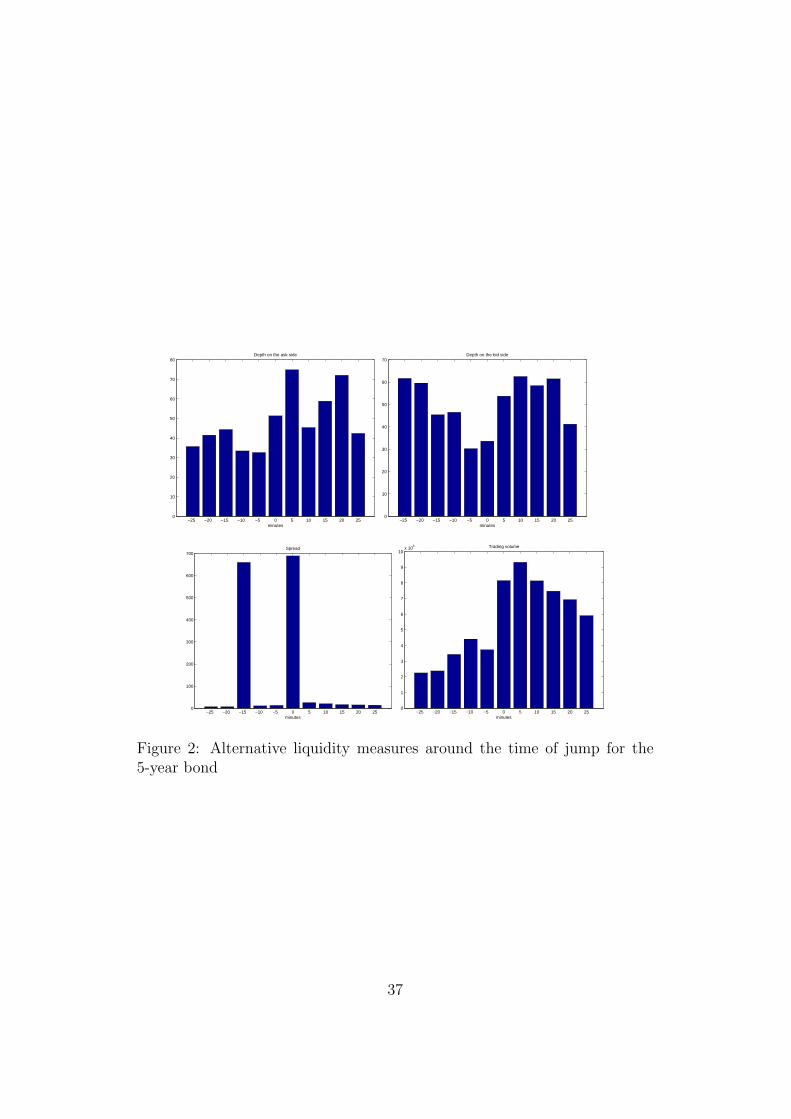
Appendix B Liquidity measures around the

time of the jump for the 5-, 10-

and 30-year US Treasury bonds

36

−25 −20 −15 −10 −5 0 5 10 15 20 250

10

20

30

40

50

60

70


minutes−25 −20 −15 −10 −5 0 5 10 15 20 25

0

10

20

30

40

50

60


minutes

−25 −20 −15 −10 −5 0 5 10 15 20 250

100

200

300

400

500

600

700Spread

minutes−25 −20 −15 −10 −5 0 5 10 15 20 25

0

1

2

3

4

5

6

7

8

9

10x 10

6 Trading volume

minutes


37

−25 −20 −15 −10 −5 0 5 10 15 20 250

5

10

15

20

25

30

35

40


minutes−25 −20 −15 −10 −5 0 5 10 15 20 25

0

10

20

30

40

50


minutes

−25 −20 −15 −10 −5 0 5 10 15 20 250

100

200

300

400

500

600

700Spread

minutes−25 −20 −15 −10 −5 0 5 10 15 20 25

0

1

2

3

4

5

6

7x 10

6 Trading volume

minutes


38

−25 −20 −15 −10 −5 0 5 10 15 20 250

1

2

3

4

5

6


minutes−25 −20 −15 −10 −5 0 5 10 15 20 25

0

0.5

1

1.5

2

2.5

3

3.5

4

4.5Depth on the bid side

minutes

−25 −20 −15 −10 −5 0 5 10 15 20 25−800

−700

−600

−500

−400

−300

−200

−100

0Spread

minutes−25 −20 −15 −10 −5 0 5 10 15 20 25

0

2

4

6

8

10

12x 10

4 Trading volume

minutes


39

Appendix C More results on the price for-

mation process when jumps oc-

cur

40

Model 1

Coefficient Std. Error t-Statistic p-valueα -0.0257 0.1051 -0.24 0.8069

φJ -0.7431 0.5968 -1.25 0.2131θJ 3.8223 0.5850 6.53 0.0000

φNJ -1.1816 0.2124 -5.56 0.0000θNJ 3.4496 0.2053 16.80 0.0000

Model 2 Model 3

Coefficient Std. Error t-Statistic p-value Coefficient Std. Error t-Statistic p-valueα -0.0237 0.1049 -0.23 0.8215 α -0.0273 0.1045 -0.26 0.7938

φJ0 -24.9491 17.4855 -1.43 0.1536 φJ0 -24.9511 17.7134 -1.41 0.1590θJ0 16.9362 13.7566 1.23 0.2183 θJ0 19.1459 13.8811 1.38 0.1678φB 0.6611 1.1087 0.60 0.5510 φB5 -0.2331 6.8353 -0.03 0.9728θB 2.9124 1.0484 2.78 0.0055 θB5 6.5974 2.3795 2.77 0.0056φA -0.8181 0.7015 -1.17 0.2436 φA5 -4.7729 15.2462 -0.31 0.7542θA 3.7285 0.6788 5.49 0.0000 θA5 23.9930 15.0539 1.59 0.1110


Model 4 Model 5

Coefficient Std. Error t-Statistic p-value Coefficient Std. Error t-Statistic p-valueα -0.0239 0.1044 -0.23 0.8190 α -0.0282 0.1045 -0.27 0.7875

φJ0 -24.9523 17.7136 -1.41 0.1589 φJ0 -24.0574 17.2641 -1.39 0.1635θJ0 19.1466 13.8809 1.38 0.1678 θJ0 14.9826 13.0245 1.15 0.2500




41

Model 2 Model 3


φJ0 -0.1817 0.7828 -0.23 0.8164 φJ0 -0.1950 0.7817 -0.25 0.8030θJ0 1.1431 0.5225 2.19 0.0287 θJ0 1.6079 0.5288 3.04 0.0024φB -0.0606 0.0870 -0.70 0.4865 φB5 -0.6672 0.9869 -0.68 0.4990θB 1.0102 0.0911 11.09 0.0000 θB5 2.1253 1.1136 1.91 0.0563φA -0.0927 0.0413 -2.25 0.0247 φA5 0.0205 0.3248 0.06 0.9497θA 1.2527 0.0402 31.15 0.0000 θA5 1.3736 0.3089 4.45 0.0000


Model 4 Model 5


φJ0 -0.1597 0.7964 -0.20 0.8411 φJ0 -0.1475 0.8011 -0.18 0.8540θJ0 1.2609 0.5186 2.43 0.0151 θJ0 1.0923 0.5119 2.13 0.0328

φB10 -0.3350 0.7356 -0.46 0.6488 φB20 -0.6106 0.4776 -1.28 0.2010θB10 1.7748 0.6770 2.62 0.0088 θB20 1.8977 0.5145 3.69 0.0002φA10 0.0997 0.2567 0.39 0.6978 φA20 0.1240 0.1614 0.77 0.4422θA10 1.3958 0.2513 5.55 0.0000 θA20 1.3062 0.1535 8.51 0.0000


Table 12: Estimated coefficients, standard errors, t-statistics and p-values, respectively, for Models 2-5 for the 10-yearbond, for a ‘jump window’ of -/+ 5 minutes. The other time windows around the jump time are adjusted accordingly tothe ‘jump window’. For instance, for Model 3, which considers a -/+ 5 minutes window around the jumps, the before andafter windows are of -/+ 10 minutes around the jump time, as identified in Section 2.2.2. For all models, the value of thecorrelation coefficient for the order flow is ρ = 0.6609.

42

Model 1


φJ 0.0189 0.0143 1.32 0.1872θJ 0.3880 0.0122 31.81 0.0000

φNJ 0.0478 0.0040 11.91 0.0000θNJ 0.3237 0.0036 90.58 0.0000

Model 2 Model 3


φJ0 -0.7647 0.5206 -1.47 0.1419 φJ0 -0.7454 0.5193 -1.44 0.1512θJ0 1.2906 0.4030 3.20 0.0014 θJ0 1.4301 0.3989 3.59 0.0003φB 0.0576 0.0249 2.31 0.0209 φB5 0.1959 0.1394 1.40 0.1600θB 0.2935 0.0199 14.76 0.0000 θB5 0.3398 0.0596 5.70 0.0000φA 0.0178 0.0127 1.39 0.1635 φA5 -0.2651 0.1397 -1.90 0.0577θA 0.3734 0.0115 32.43 0.0000 θA5 0.7977 0.1128 7.07 0.0000

φNJ 0.0478 0.0040 11.91 0.0000 φother 0.0463 0.0038 12.26 0.0000θNJ 0.3236 0.0036 90.58 0.0000 θother 0.3290 0.0034 97.70 0.0000

Model 4 Model 5


φJ0 -0.7453 0.5193 -1.44 0.1512 φJ0 -0.7520 0.5212 -1.44 0.1491θJ0 1.4308 0.3989 3.59 0.0003 θJ0 1.3293 0.4043 3.29 0.0010


φother 0.0472 0.0038 12.50 0.0000 φother 0.0483 0.0038 12.74 0.0000θother 0.3273 0.0034 97.58 0.0000 θother 0.3252 0.0034 96.68 0.0000

Table 13: Estimated coefficients, standard errors, t-statistics and p-values, respectively, for Models 1-5 for the 2-yearbond. We use different values for the autocorrelation coefficient for the order flow, as resulting from Table 10.

43

Documents

C:/Users/Ana-Maria/OneDrive/paper2/Paper2 10 Jan 2015 and Information...School, London, 4-5 September 2014) in particular Neil R. Ericsson, Sir David Hendry, ... JEL classiﬁcation