Embed Size (px)
Citation preview
SAS/STAT® 14.2 User’s GuideCustomizing theKaplan-Meier SurvivalPlot
This document is an individual chapter from SAS/STAT® 14.2 User’s Guide.
The correct bibliographic citation for this manual is as follows: SAS Institute Inc. 2016. SAS/STAT® 14.2 User’s Guide. Cary, NC:SAS Institute Inc.
SAS/STAT® 14.2 User’s Guide
Copyright © 2016, SAS Institute Inc., Cary, NC, USA
All Rights Reserved. Produced in the United States of America.
For a hard-copy book: No part of this publication may be reproduced, stored in a retrieval system, or transmitted, in any form or byany means, electronic, mechanical, photocopying, or otherwise, without the prior written permission of the publisher, SAS InstituteInc.
For a web download or e-book: Your use of this publication shall be governed by the terms established by the vendor at the timeyou acquire this publication.
The scanning, uploading, and distribution of this book via the Internet or any other means without the permission of the publisher isillegal and punishable by law. Please purchase only authorized electronic editions and do not participate in or encourage electronicpiracy of copyrighted materials. Your support of others’ rights is appreciated.
U.S. Government License Rights; Restricted Rights: The Software and its documentation is commercial computer softwaredeveloped at private expense and is provided with RESTRICTED RIGHTS to the United States Government. Use, duplication, ordisclosure of the Software by the United States Government is subject to the license terms of this Agreement pursuant to, asapplicable, FAR 12.212, DFAR 227.7202-1(a), DFAR 227.7202-3(a), and DFAR 227.7202-4, and, to the extent required under U.S.federal law, the minimum restricted rights as set out in FAR 52.227-19 (DEC 2007). If FAR 52.227-19 is applicable, this provisionserves as notice under clause (c) thereof and no other notice is required to be affixed to the Software or documentation. TheGovernment’s rights in Software and documentation shall be only those set forth in this Agreement.
SAS Institute Inc., SAS Campus Drive, Cary, NC 27513-2414
November 2016
SAS® and all other SAS Institute Inc. product or service names are registered trademarks or trademarks of SAS Institute Inc. in theUSA and other countries. ® indicates USA registration.
Other brand and product names are trademarks of their respective companies.
SAS software may be provided with certain third-party software, including but not limited to open-source software, which islicensed under its applicable third-party software license agreement. For license information about third-party software distributedwith SAS software, refer to http://support.sas.com/thirdpartylicenses.
Chapter 23
Customizing the Kaplan-Meier Survival Plot
ContentsOverview . . . . . . . . . . . . . . . . . . . . . . . . . . . . . . . . . . . . . . . . . . . . 806Controlling the Survival Plot by Specifying Procedure Options . . . . . . . . . . . . . . . . 807
Enabling ODS Graphics and the Default Kaplan-Meier Plot . . . . . . . . . . . . . . 807Individual Survival Plots . . . . . . . . . . . . . . . . . . . . . . . . . . . . . . . . . 809Hall-Wellner Confidence Bands and Homogeneity Test . . . . . . . . . . . . . . . . . 811Equal-Precision Bands . . . . . . . . . . . . . . . . . . . . . . . . . . . . . . . . . . 812Displaying the Patients-at-Risk Table inside the Plot . . . . . . . . . . . . . . . . . . 814Displaying the Patients-at-Risk Table outside the Plot . . . . . . . . . . . . . . . . . 816Modifying At-Risk Table Times . . . . . . . . . . . . . . . . . . . . . . . . . . . . . 817Reordering the Groups . . . . . . . . . . . . . . . . . . . . . . . . . . . . . . . . . . 820Suppressing the Censored Observations . . . . . . . . . . . . . . . . . . . . . . . . . 823Failure Plots . . . . . . . . . . . . . . . . . . . . . . . . . . . . . . . . . . . . . . . 824
Controlling the Survival Plot by Modifying Graph Templates . . . . . . . . . . . . . . . . . 824The Modularized Templates . . . . . . . . . . . . . . . . . . . . . . . . . . . . . . . 825Changing the Plot Title . . . . . . . . . . . . . . . . . . . . . . . . . . . . . . . . . . 827Modifying the Axis . . . . . . . . . . . . . . . . . . . . . . . . . . . . . . . . . . . 829Changing the Line Thickness . . . . . . . . . . . . . . . . . . . . . . . . . . . . . . 831Changing the Group Color . . . . . . . . . . . . . . . . . . . . . . . . . . . . . . . . 832Changing the Line Pattern . . . . . . . . . . . . . . . . . . . . . . . . . . . . . . . . 833Changing the Font . . . . . . . . . . . . . . . . . . . . . . . . . . . . . . . . . . . . 834Changing the Legend and Inset Position . . . . . . . . . . . . . . . . . . . . . . . . . 836Changing How the Censored Points Are Displayed . . . . . . . . . . . . . . . . . . . 838Adding a Y-Axis Reference Line . . . . . . . . . . . . . . . . . . . . . . . . . . . . 839Changing the Homogeneity Test Inset . . . . . . . . . . . . . . . . . . . . . . . . . . 841Suppressing the Second Title and Adding a Footnote . . . . . . . . . . . . . . . . . . 843Adding a Small Inset Table with Event Information . . . . . . . . . . . . . . . . . . . 844Adding an External Table with Event Information . . . . . . . . . . . . . . . . . . . 846Suppressing the Legend . . . . . . . . . . . . . . . . . . . . . . . . . . . . . . . . . 848Kaplan-Meier Plot with Event Table and Other Customizations . . . . . . . . . . . . 849Compiled Template Cleanup . . . . . . . . . . . . . . . . . . . . . . . . . . . . . . . 850
Graph Templates, Macros, and Macro Variables . . . . . . . . . . . . . . . . . . . . . . . . 851The Macro Variables . . . . . . . . . . . . . . . . . . . . . . . . . . . . . . . . . . . 853The Smaller Macros . . . . . . . . . . . . . . . . . . . . . . . . . . . . . . . . . . . 856The Larger Macros . . . . . . . . . . . . . . . . . . . . . . . . . . . . . . . . . . . . 856Event Table Macros . . . . . . . . . . . . . . . . . . . . . . . . . . . . . . . . . . . 861
806 F Chapter 23: Customizing the Kaplan-Meier Survival Plot
Dynamic Variables . . . . . . . . . . . . . . . . . . . . . . . . . . . . . . . . . . . . . . . 863Dynamic Variables That Are Automatically Declared . . . . . . . . . . . . . . . . . . 863Additional Dynamic Variables . . . . . . . . . . . . . . . . . . . . . . . . . . . . . . 864
Style Templates . . . . . . . . . . . . . . . . . . . . . . . . . . . . . . . . . . . . . . . . . 865Changing the Style . . . . . . . . . . . . . . . . . . . . . . . . . . . . . . . . . . . . 866Color Priority Styles . . . . . . . . . . . . . . . . . . . . . . . . . . . . . . . . . . . 867Displaying a Style and Extracting Color Lists . . . . . . . . . . . . . . . . . . . . . . 868Modifying Color Lists . . . . . . . . . . . . . . . . . . . . . . . . . . . . . . . . . . 871Swapping Colors among Style Elements . . . . . . . . . . . . . . . . . . . . . . . . 872Displaying a Style and Extracting Font Information . . . . . . . . . . . . . . . . . . 874Displaying Other Style Elements . . . . . . . . . . . . . . . . . . . . . . . . . . . . 876
SAS Item Stores . . . . . . . . . . . . . . . . . . . . . . . . . . . . . . . . . . . . . . . . 879References . . . . . . . . . . . . . . . . . . . . . . . . . . . . . . . . . . . . . . . . . . . 879
OverviewThe LIFETEST procedure is a nonparametric procedure for analyzing survival data. You can use PROCLIFETEST to compute the Kaplan-Meier curve (1958), which is a nonparametric maximum likelihoodestimate of the survivor function. The Kaplan-Meier plot (also called the product-limit survival plot) is apopular tool in medical, pharmaceutical, and life sciences research. The Kaplan-Meier plot contains stepfunctions that represent the Kaplan-Meier curves of different samples (strata). The Kaplan-Meier plot hasmany other features that you can add or change through procedure options, graph templates, and styletemplates. This chapter explores these features in detail but does not explain how to interpret the graphsor the underlying analysis. For more information about PROC LIFETEST and the Kaplan-Meier plot, seeChapter 71, “The LIFETEST Procedure.”
This chapter shows you how to modify the Kaplan-Meier plot through a series of examples. It discussesfour types of examples: specifying procedure options, modifying graph templates by using macro variables,modifying graph templates by using macros, and changing styles. Most examples do not go into detail aboutthe tools that underlie the template changes. Each example is designed to be small, simple, self-contained,and easy to copy and use “as is” or with minor modifications. Subsequent sections provide more detailsabout the macro variables and macros that are used to modify the graph templates. You can use the simpleexamples to make a wide variety of changes without reading or understanding the detailed descriptions at theend of this chapter.
Statistical procedures produce tables by using the Output Delivery System (ODS) and produce graphs byusing ODS Graphics. Procedures produce graphs as automatically as they produce tables, and graphs andtables are integrated in the ODS output. Graphs that are produced by ODS Graphics are controlled by options,the data object (the matrix of information that is graphed), a style template, and a graph template. A styletemplate is a SAS program that controls the overall appearance of graphs, including colors, line and markerstyles, sizes, fonts, and so on. A graph template is a SAS program, written in the Graph Template Language
Controlling the Survival Plot by Specifying Procedure Options F 807
(GTL), that provides a detailed specification of the layout and contents of each graph. Each graph that iscreated when ODS Graphics is enabled is controlled by a graph template.1
If you want to modify a graph template, you usually use the TEMPLATE procedure to display the templateof interest, and then you copy it into your editor, modify it, and submit it to SAS to compile. Then, when yourun your procedure, it uses the new template. The PROC LIFETEST survival plot is the only plot in SASfor which you have another alternative available for template modification. SAS provides the survival plottemplates in a series of macros and macro variables that are modular and easier to modify than the originaltemplates. This chapter provides numerous examples of using these macros and macro variables.
The data that are used in this chapter come from 137 bone marrow transplant patients in a study by Klein andMoeschberger (1997) and are available in the BMT data set in the Sashelp library. At the time of transplant,each patient is classified in one of three risk categories: ALL (acute lymphoblastic leukemia), AML (acutemyelocytic leukemia)–Low Risk, and AML–High Risk. The endpoint of interest is the disease-free survivaltime, which is the time in days until death, relapse, or the end of the study. The variable Group represents thepatient’s risk category, the variable T represents the disease-free survival time, and the variable Status is thecensoring indicator. A status of 1 indicates an event time, and a status of 0 indicates a censored time.
Controlling the Survival Plot by Specifying Procedure OptionsThis section provides a series of examples that use ODS Graphics and the PLOTS= option in the PROCLIFETEST statement to control the appearance of the survival plot. Other examples use formats and theORDER= option to control the order of the groups.
Enabling ODS Graphics and the Default Kaplan-Meier PlotYou can use the following statements to enable ODS Graphics and run PROC LIFETEST:
ods graphics on;
proc lifetest data=sashelp.BMT;time T * Status(0);strata Group;
run;
ODS Graphics is enabled for this step and all subsequent steps until it is disabled. ODS Graphics remainsenabled throughout the examples in this chapter.
You specify in the TIME statement that the disease-free survival time is recorded in the variable T. Youfurther specify that the variable Status indicates censoring and 0 indicates a censored time. Separate survivorfunctions are displayed for each group in the Group variable, which you specify in the STRATA statement.
The plot in Figure 23.1 consists of three step functions, one for each of the three groups of patients. The plotshows that patients in the AML–Low Risk group have longer disease-free survival than patients in the ALLand AML–High Risk groups.
1ODS Graphics might or might not be enabled by default. ODS Graphics is usually enabled by default in the SAS windowingenvironment and disabled when you invoke SAS in other ways. However, these defaults can be changed in a number of ways. ODSGraphics is enabled in the first example in this chapter by the ODS GRAPHICS ON statement and remains enabled throughout thechapter.

808 F Chapter 23: Customizing the Kaplan-Meier Survival Plot
Figure 23.1 Default Kaplan-Meier Plot
The following step, which explicitly specifies the default PLOTS=SURVIVAL option, is equivalent to thepreceding step:
proc lifetest data=sashelp.BMT plots=survival;time T * Status(0);strata Group;
run;
The PLOTS= option enables you to control the graphs that a procedure produces. You can use it to requestnondefault graphs and specify options for some graphs. You can specify graph names (PLOTS=SURVIVAL),graph options (PLOTS=SURVIVAL(ATRISK OUTSIDE)), and suboptions (PLOTS=SURVIVAL(ATRISKOUTSIDE(0.15))). The PLOTS= option is described in the section “PROC LIFETEST Statement” onpage 5215 in Chapter 71, “The LIFETEST Procedure.”
Individual Survival Plots F 809
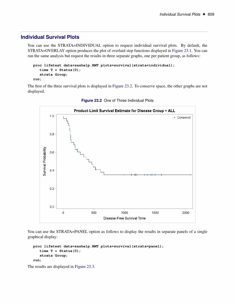
Individual Survival PlotsYou can use the STRATA=INDIVIDUAL option to request individual survival plots. By default, theSTRATA=OVERLAY option produces the plot of overlaid step functions displayed in Figure 23.1. You canrun the same analysis but request the results in three separate graphs, one per patient group, as follows:
proc lifetest data=sashelp.BMT plots=survival(strata=individual);time T * Status(0);strata Group;
run;
The first of the three survival plots is displayed in Figure 23.2. To conserve space, the other graphs are notdisplayed.
Figure 23.2 One of Three Individual Plots
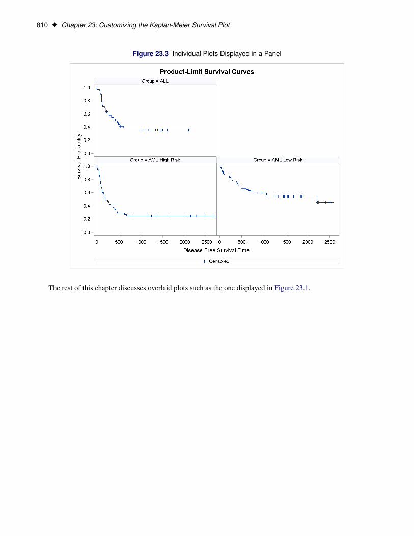
You can use the STRATA=PANEL option as follows to display the results in separate panels of a singlegraphical display:
proc lifetest data=sashelp.BMT plots=survival(strata=panel);time T * Status(0);strata Group;
run;
The results are displayed in Figure 23.3.
810 F Chapter 23: Customizing the Kaplan-Meier Survival Plot
Figure 23.3 Individual Plots Displayed in a Panel
The rest of this chapter discusses overlaid plots such as the one displayed in Figure 23.1.
Hall-Wellner Confidence Bands and Homogeneity Test F 811
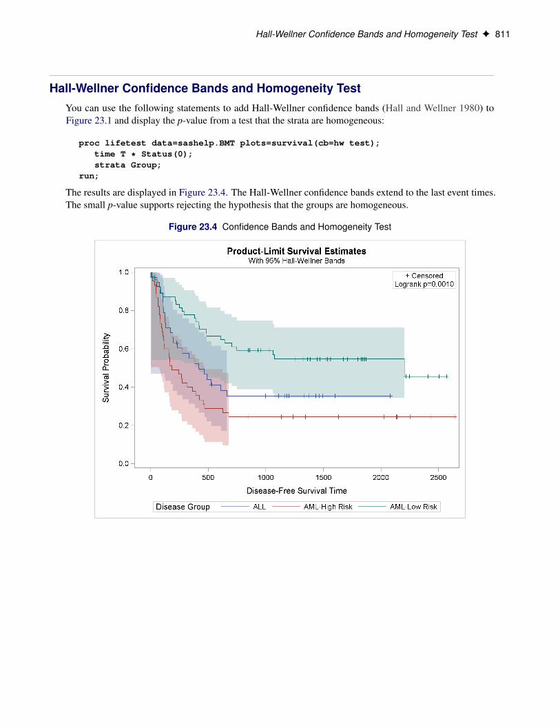
Hall-Wellner Confidence Bands and Homogeneity TestYou can use the following statements to add Hall-Wellner confidence bands (Hall and Wellner 1980) toFigure 23.1 and display the p-value from a test that the strata are homogeneous:
proc lifetest data=sashelp.BMT plots=survival(cb=hw test);time T * Status(0);strata Group;
run;
The results are displayed in Figure 23.4. The Hall-Wellner confidence bands extend to the last event times.The small p-value supports rejecting the hypothesis that the groups are homogeneous.
Figure 23.4 Confidence Bands and Homogeneity Test

812 F Chapter 23: Customizing the Kaplan-Meier Survival Plot
Equal-Precision BandsYou can use the following statements to add equal-precision bands to the plot:
proc lifetest data=sashelp.BMT plots=survival(cb=ep test);time T * Status(0);strata Group;
run;
The results are displayed in Figure 23.5.
Figure 23.5 Equal-Precision Bands
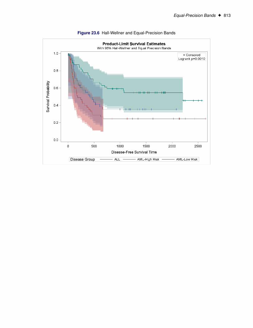
You can use the following statements to add both Hall-Wellner and equal-precision bands to the plot:
proc lifetest data=sashelp.BMT plots=survival(cb=all test);time T * Status(0);strata Group;
run;
The results are displayed in Figure 23.6.
Equal-Precision Bands F 813
Figure 23.6 Hall-Wellner and Equal-Precision Bands
814 F Chapter 23: Customizing the Kaplan-Meier Survival Plot
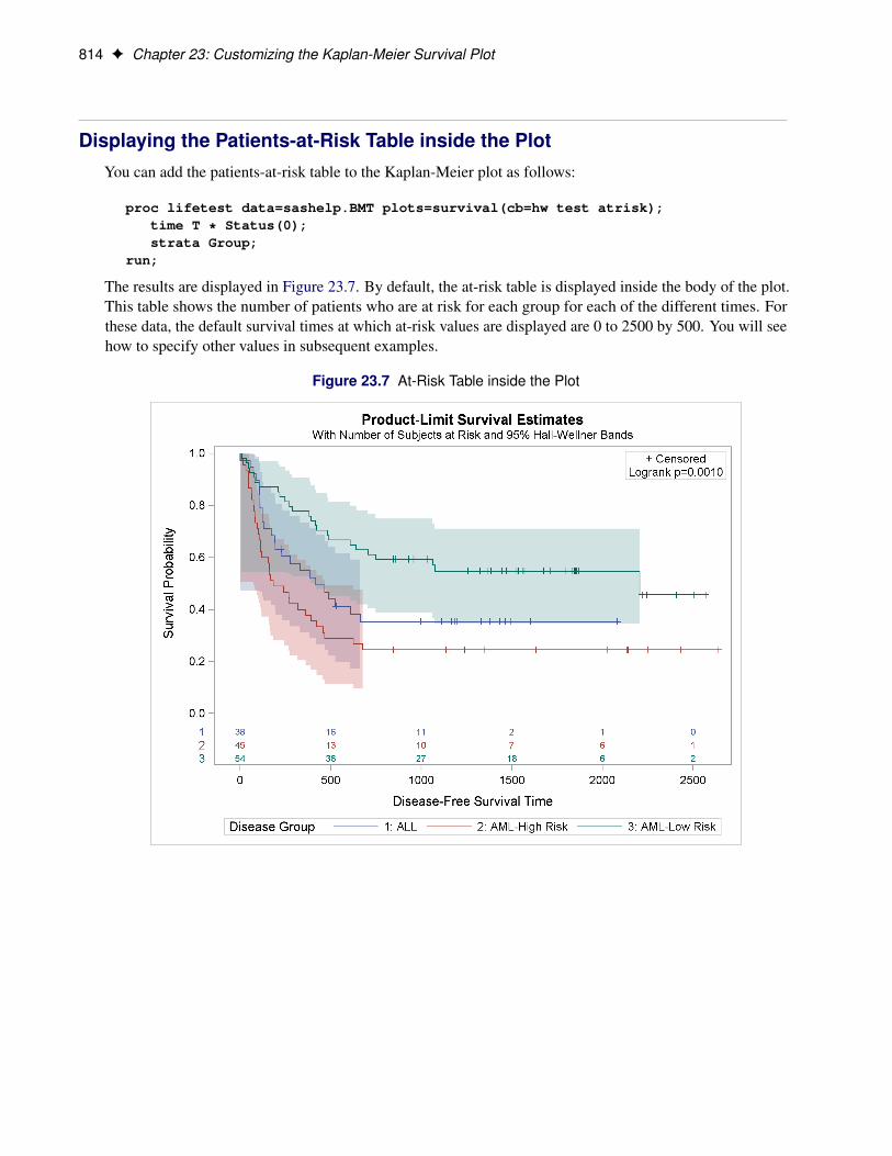
Displaying the Patients-at-Risk Table inside the PlotYou can add the patients-at-risk table to the Kaplan-Meier plot as follows:
proc lifetest data=sashelp.BMT plots=survival(cb=hw test atrisk);time T * Status(0);strata Group;
run;
The results are displayed in Figure 23.7. By default, the at-risk table is displayed inside the body of the plot.This table shows the number of patients who are at risk for each group for each of the different times. Forthese data, the default survival times at which at-risk values are displayed are 0 to 2500 by 500. You will seehow to specify other values in subsequent examples.
Figure 23.7 At-Risk Table inside the Plot
Displaying the Patients-at-Risk Table inside the Plot F 815
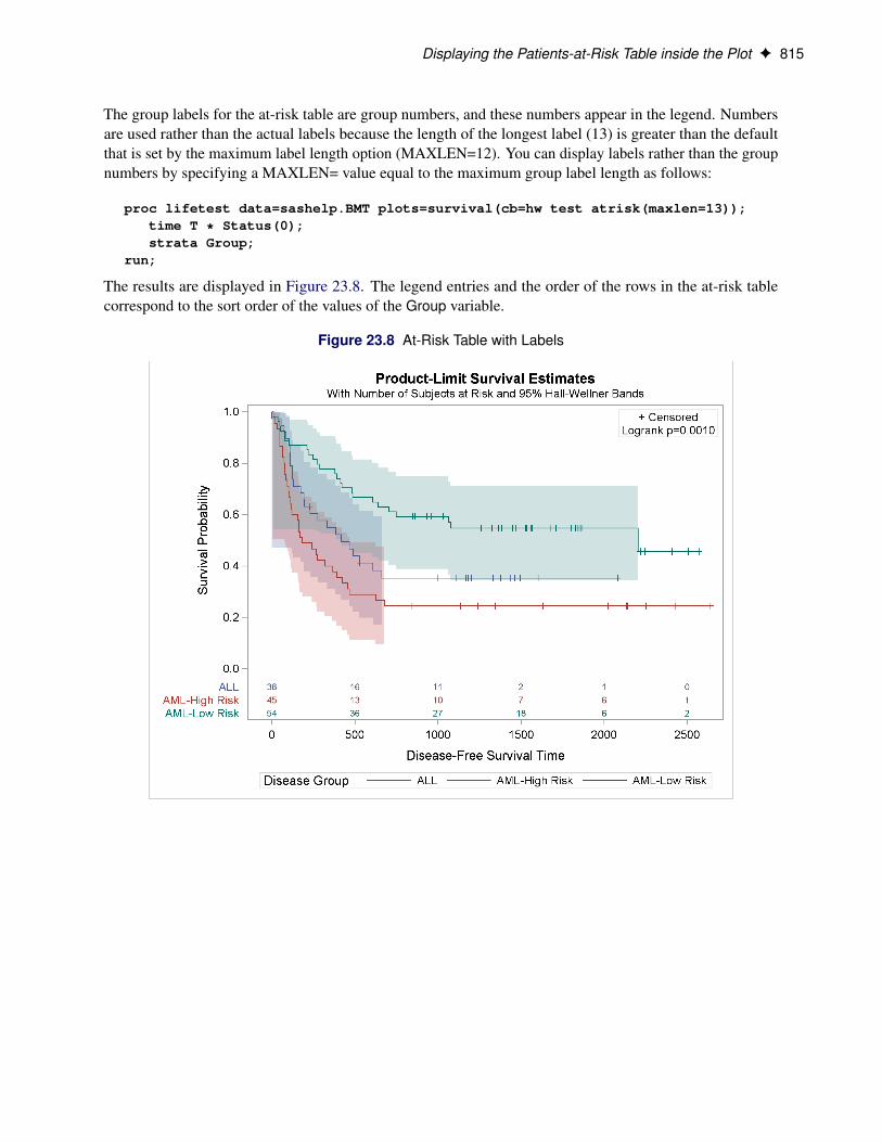
The group labels for the at-risk table are group numbers, and these numbers appear in the legend. Numbersare used rather than the actual labels because the length of the longest label (13) is greater than the defaultthat is set by the maximum label length option (MAXLEN=12). You can display labels rather than the groupnumbers by specifying a MAXLEN= value equal to the maximum group label length as follows:
proc lifetest data=sashelp.BMT plots=survival(cb=hw test atrisk(maxlen=13));time T * Status(0);strata Group;
run;
The results are displayed in Figure 23.8. The legend entries and the order of the rows in the at-risk tablecorrespond to the sort order of the values of the Group variable.
Figure 23.8 At-Risk Table with Labels
816 F Chapter 23: Customizing the Kaplan-Meier Survival Plot
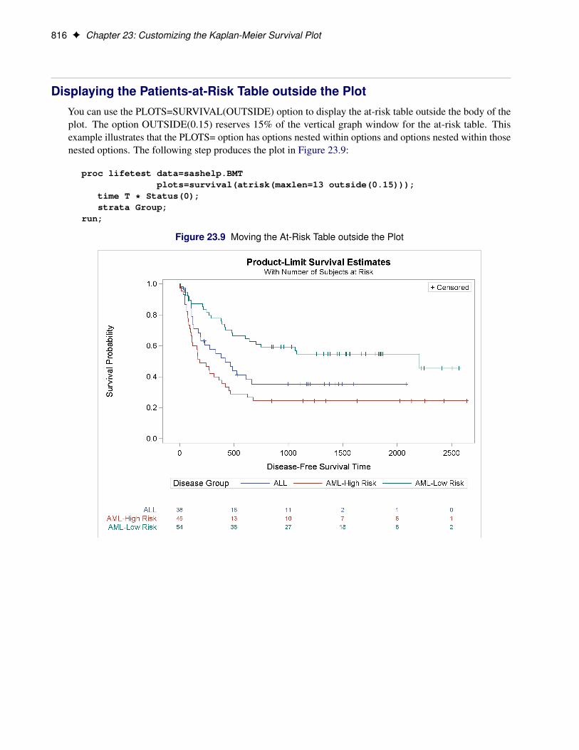
Displaying the Patients-at-Risk Table outside the PlotYou can use the PLOTS=SURVIVAL(OUTSIDE) option to display the at-risk table outside the body of theplot. The option OUTSIDE(0.15) reserves 15% of the vertical graph window for the at-risk table. Thisexample illustrates that the PLOTS= option has options nested within options and options nested within thosenested options. The following step produces the plot in Figure 23.9:
proc lifetest data=sashelp.BMTplots=survival(atrisk(maxlen=13 outside(0.15)));
time T * Status(0);strata Group;
run;
Figure 23.9 Moving the At-Risk Table outside the Plot
Modifying At-Risk Table Times F 817
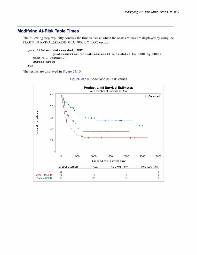
Modifying At-Risk Table TimesThe following step explicitly controls the time values at which the at-risk values are displayed by using thePLOTS=SURVIVAL(ATRISK=0 TO 3000 BY 1000) option:
proc lifetest data=sashelp.BMTplots=survival(atrisk(maxlen=13 outside)=0 to 3000 by 1000);
time T * Status(0);strata Group;
run;
The results are displayed in Figure 23.10.
Figure 23.10 Specifying At-Risk Values
818 F Chapter 23: Customizing the Kaplan-Meier Survival Plot
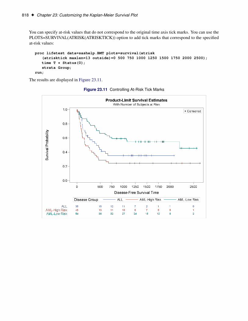
You can specify at-risk values that do not correspond to the original time axis tick marks. You can use thePLOTS=SURVIVAL(ATRISK(ATRISKTICK)) option to add tick marks that correspond to the specifiedat-risk values:
proc lifetest data=sashelp.BMT plots=survival(atrisk(atrisktick maxlen=13 outside)=0 500 750 1000 1250 1500 1750 2000 2500);time T * Status(0);strata Group;
run;
The results are displayed in Figure 23.11.
Figure 23.11 Controlling At-Risk Tick Marks
Modifying At-Risk Table Times F 819
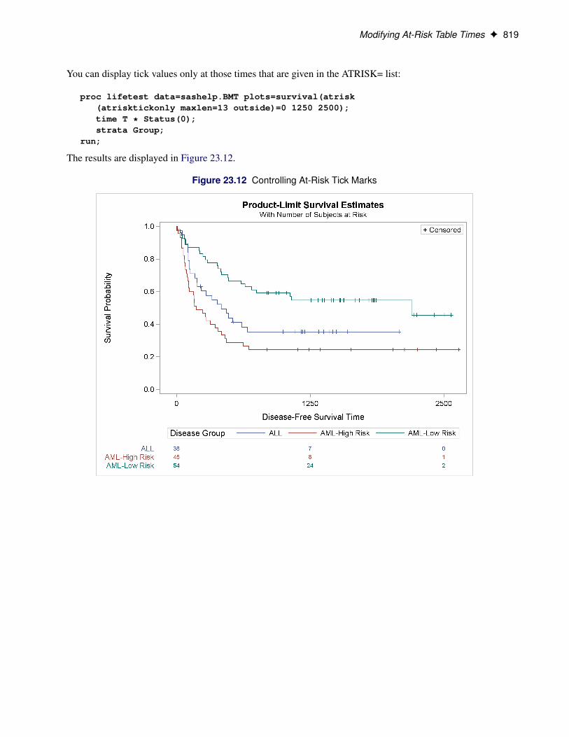
You can display tick values only at those times that are given in the ATRISK= list:
proc lifetest data=sashelp.BMT plots=survival(atrisk(atrisktickonly maxlen=13 outside)=0 1250 2500);time T * Status(0);strata Group;
run;
The results are displayed in Figure 23.12.
Figure 23.12 Controlling At-Risk Tick Marks
820 F Chapter 23: Customizing the Kaplan-Meier Survival Plot
Reordering the GroupsYou can change the order of the legend entries by first changing each original group value to a new value inthe desired order and then running the analysis with a FORMAT statement to provide the original values.In this example, the order is changed to AML–Low Risk (the top function), followed by ALL (the middlefunction), followed by AML–High Risk. With this ordering, there is a clearer correspondence between thefunctions, the at-risk table, and the legend. The following steps illustrate this reordering:
proc format;invalue bmtnum 'AML-Low Risk' = 1 'ALL' = 2 'AML-High Risk' = 3;value bmtfmt 1 = 'AML-Low Risk' 2 = 'ALL' 3 = 'AML-High Risk';
run;
data BMT(drop=g);set sashelp.BMT(rename=(group=g));Group = input(g, bmtnum.);
run;
proc lifetest data=BMT plots=survival(cl test atrisk(maxlen=13));time T * Status(0);strata Group / order=internal;format group bmtfmt.;
run;
The PROC FORMAT step has two statements. The INVALUE statement creates an informat that maps thevalues of the original Group variable into integers that have the correct order. The VALUE statement createsa format that maps the integers back to the original values. The informat is used with the INPUT functionin the DATA step to create a new integer Group variable. The FORMAT statement assigns the BMTFMTformat to the Group variable so that the actual risk groups are displayed in the analysis. You specify theORDER=INTERNAL option in the STRATA statement to sort the Group values based on internal order (theorder specified by the integers, which are the internal unformatted values). This example also illustrates theCL option, which displays pointwise confidence limits for the survival curve (instead of the Hall-Wellnerconfidence bands). The results are displayed in Figure 23.13.
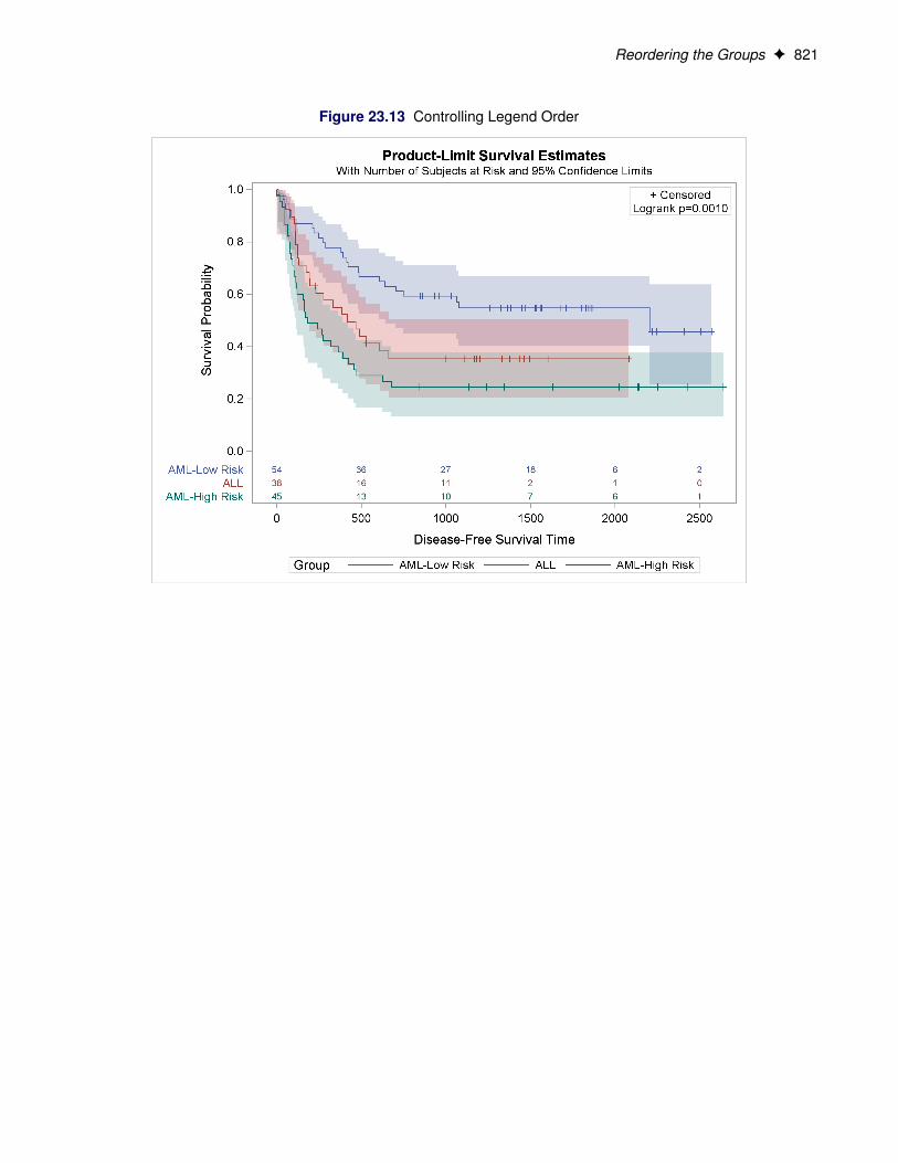
Reordering the Groups F 821
Figure 23.13 Controlling Legend Order
822 F Chapter 23: Customizing the Kaplan-Meier Survival Plot
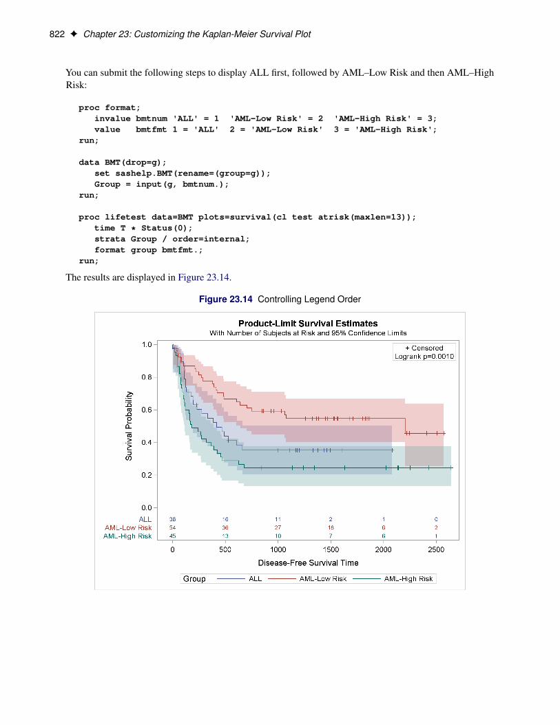
You can submit the following steps to display ALL first, followed by AML–Low Risk and then AML–HighRisk:
proc format;invalue bmtnum 'ALL' = 1 'AML-Low Risk' = 2 'AML-High Risk' = 3;value bmtfmt 1 = 'ALL' 2 = 'AML-Low Risk' 3 = 'AML-High Risk';
run;
data BMT(drop=g);set sashelp.BMT(rename=(group=g));Group = input(g, bmtnum.);
run;
proc lifetest data=BMT plots=survival(cl test atrisk(maxlen=13));time T * Status(0);strata Group / order=internal;format group bmtfmt.;
run;
The results are displayed in Figure 23.14.
Figure 23.14 Controlling Legend Order
Suppressing the Censored Observations F 823
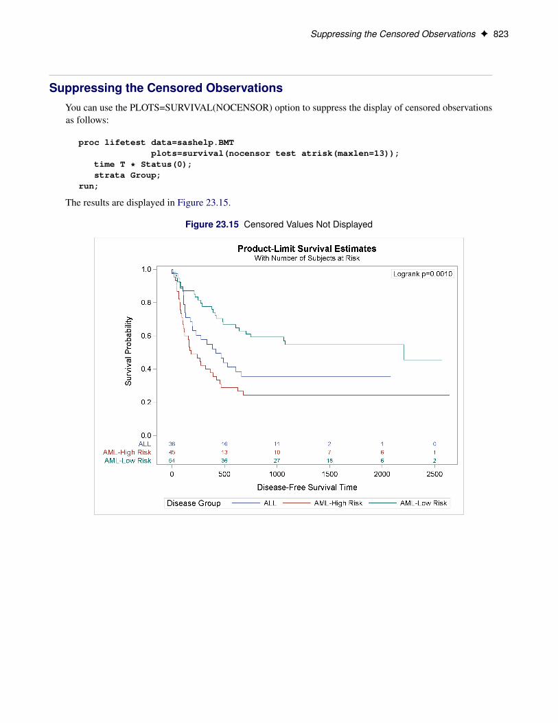
Suppressing the Censored ObservationsYou can use the PLOTS=SURVIVAL(NOCENSOR) option to suppress the display of censored observationsas follows:
proc lifetest data=sashelp.BMTplots=survival(nocensor test atrisk(maxlen=13));
time T * Status(0);strata Group;
run;
The results are displayed in Figure 23.15.
Figure 23.15 Censored Values Not Displayed
824 F Chapter 23: Customizing the Kaplan-Meier Survival Plot
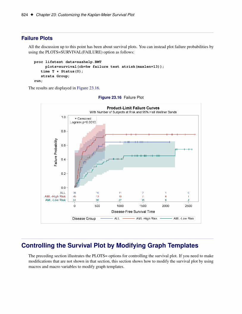
Failure PlotsAll the discussion up to this point has been about survival plots. You can instead plot failure probabilities byusing the PLOTS=SURVIVAL(FAILURE) option as follows:
proc lifetest data=sashelp.BMTplots=survival(cb=hw failure test atrisk(maxlen=13));
time T * Status(0);strata Group;
run;
The results are displayed in Figure 23.16.
Figure 23.16 Failure Plot
Controlling the Survival Plot by Modifying Graph TemplatesThe preceding section illustrates the PLOTS= options for controlling the survival plot. If you need to makemodifications that are not shown in that section, this section shows how to modify the survival plot by usingmacros and macro variables to modify graph templates.
The Modularized Templates F 825
The Modularized TemplatesSAS provides the two templates that are used to make the survival plot in a modularized form.2 Themodularized version of the two survival plot templates is available in the SAS sample library and ison the Web at http://support.sas.com/documentation/onlinedoc/stat/ex_code/142/templft.html.
The file defines the macro %ProvideSurvivalMacros, which defines a series of macros and macro variables.The %ProvideSurvivalMacros macro contains a %GLOBAL statement, a series of %LET statements, andseveral macro definitions. It ends with a call to the %CompileSurvivalTemplates macro (which is definedinside the %ProvideSurvivalMacros macro), which compiles the two survival plot templates.3 By usingthese macros and macro variables, you can easily specify single changes that modify both templates. All thestatements in this file are displayed and explained in more detail in the section “Graph Templates, Macros,and Macro Variables” on page 851.
The %ProvideSurvivalMacros macro provides a way to provide (and in subsequent steps restore) the defaultmacros and macro variables. The macros and macro variables are designed so that you can make mostchanges by submitting just a few lines of SAS code. Hence, you should not modify any of the statementswhile they are inside the %ProvideSurvivalMacros macro. Rather, you should use this macro only to provideall the default macros and macro variables. You should modify the individual macros and macro variablesoutside the context of the %ProvideSurvivalMacros macro.4 The reasons for this will become clearer as youwork through the examples. Before you modify anything, you must submit the %ProvideSurvivalMacrosmacro definition from the sample library to SAS. You can both store the macros in a temporary file andsubmit them to SAS by submitting the following statements:
data _null_;%let url = //support.sas.com/documentation/onlinedoc/stat/ex_code/142;infile "http:&url/templft.html" device=url;
file 'macros.tmp';retain pre 0;input;_infile_ = tranwrd(_infile_, '&', '&');_infile_ = tranwrd(_infile_, '<' , '<');if index(_infile_, '</pre>') then pre = 0;if pre then put _infile_;if index(_infile_, '<pre>') then pre = 1;
run;
%inc 'macros.tmp' / nosource;
The TRANWRD function calls change the HTML coding of the ampersand ('&') and the less than sign'<') to the actual characters ('&' and '<').
2The two templates that PROC LIFETEST uses are named Stat.Lifetest.Graphics.ProductLimitSurvivaland Stat.Lifetest.Graphics.ProductLimitSurvival2.
3You might wonder why these macros are not simply made available in the SAS autocall library. The autocall library providesmacros that you can run. In this context, you do not need to simply run a macro. You need to copy it, extract parts of it, modify thoseparts, and submit the modified statements. That is not convenient with the autocall library.
4However, there might be something that you always want to change. For example, if you always want the survival plot to beentitled ‘Kaplan-Meier Plot’, then you can modify the title once inside the %ProvideSurvivalMacros macro. This is not illustrated inthis chapter. All examples illustrate ad hoc changes that are made outside the context of the %ProvideSurvivalMacros macro.
826 F Chapter 23: Customizing the Kaplan-Meier Survival Plot
Submitting these statements only defines the %ProvideSurvivalMacros macro. It does not make any of itscomponent macros and macro variables available. The URL macro variable is used to avoid an overly longINFILE statement.
You can provide the default macros and macro variables by running the following macro:
%ProvideSurvivalMacros
Running this macro provides the default macros and macro variables (or restores them if you have previouslysubmitted the %ProvideSurvivalMacros macro).5 The %ProvideSurvivalMacrosmacro also runs the %Com-pileSurvivalTemplates macro and hence replaces any compiled survival plot templates that you might havecreated in the past. You can recompile the templates by submitting the following macro:
%CompileSurvivalTemplates
This macro runs PROC TEMPLATE and compiles the templates from all the macros and macro variables inthe %ProvideSurvivalMacros macro along with any that you modified. Running this macro produces twocompiled templates that are stored in a special SAS data file called an item store. For more information aboutSAS item stores, see the section “SAS Item Stores” on page 879. Assuming that you have not modified yourODS path by using an ODS PATH statement, compiled templates are stored in an item store in the Sasuserlibrary. Files in the Sasuser library persist across SAS sessions until they are deleted. When you are donewith a modified template, it is wise to clean up all remnants of it by restoring the default macros and bydeleting the modified templates from the Sasuser template item store. You can delete the modified templates(so that SAS can only find the original templates) by running the following step:
proc template;delete Stat.Lifetest.Graphics.ProductLimitSurvival /
store=sasuser.templat;delete Stat.Lifetest.Graphics.ProductLimitSurvival2 /
store=sasuser.templat;run;
This step deletes the compiled templates from the item store sasuser.templat. You can omit the STORE=option if you are using the default ODS path, but it is good practice to explicitly control which templates aredeleted. Deleting the compiled templates does not change any of the macros or macro variables. Only thecompiled templates (not the macros or macro variables) affect the graph when you run PROC LIFETEST.For more information about compiled templates, item stores, and cleanup, see the section “SAS Item Stores”on page 879.
5Semicolons are not needed after a macro call like this one, so they are not used in these examples.
Changing the Plot Title F 827
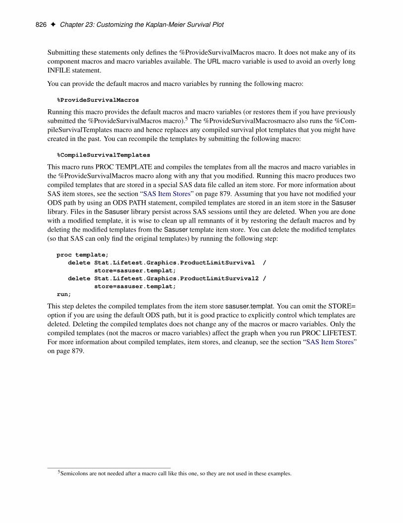
Changing the Plot TitleHere is a simple, complete program (except for retrieving the %ProvideSurvivalMacros macro from thesample library) with setup, macro variable modifications to change the title, and cleanup:
/*-- Original Macro Variable Definitions ----------------------------------%let TitleText0 = METHOD " Survival Estimate";%let TitleText1 = &titletext0 " for " STRATUMID;%let TitleText2 = &titletext0 "s";-------------------------------------------------------------------------*/
/* Make the macros and macro */%ProvideSurvivalMacros /* variables available. */
%let TitleText0 = "Kaplan-Meier Plot"; /* Change the title. */%let TitleText1 = &titletext0 " for " STRATUMID;%let TitleText2 = &titletext0;
%CompileSurvivalTemplates /* Compile the templates with *//* the new title. */
proc lifetest data=sashelp.BMT /* Perform the analysis and make */plots=survival(cb=hw test); /* the graph. */
time T * Status(0);strata Group;
run;
%ProvideSurvivalMacros /* Optionally restore the default *//* macros and macro variables. */
proc template; /* Delete the modified templates. */delete Stat.Lifetest.Graphics.ProductLimitSurvival / store=sasuser.templat;delete Stat.Lifetest.Graphics.ProductLimitSurvival2 / store=sasuser.templat;
run;
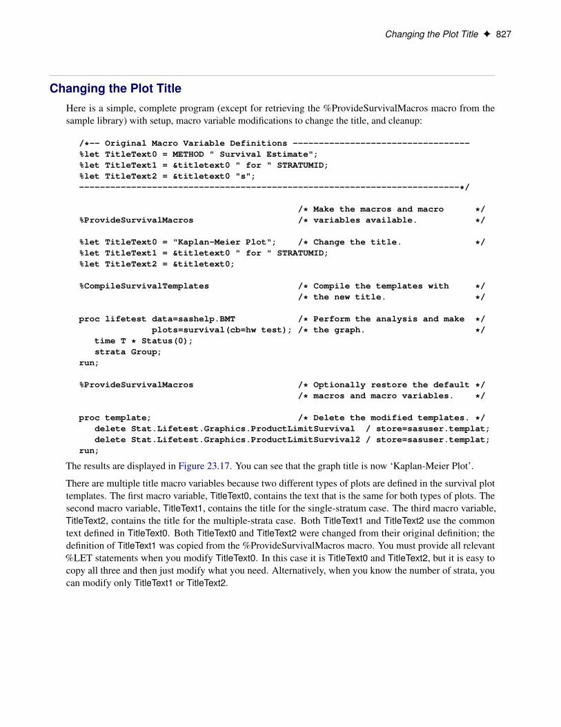
The results are displayed in Figure 23.17. You can see that the graph title is now ‘Kaplan-Meier Plot’.
There are multiple title macro variables because two different types of plots are defined in the survival plottemplates. The first macro variable, TitleText0, contains the text that is the same for both types of plots. Thesecond macro variable, TitleText1, contains the title for the single-stratum case. The third macro variable,TitleText2, contains the title for the multiple-strata case. Both TitleText1 and TitleText2 use the commontext defined in TitleText0. Both TitleText0 and TitleText2 were changed from their original definition; thedefinition of TitleText1 was copied from the %ProvideSurvivalMacros macro. You must provide all relevant%LET statements when you modify TitleText0. In this case it is TitleText0 and TitleText2, but it is easy tocopy all three and then just modify what you need. Alternatively, when you know the number of strata, youcan modify only TitleText1 or TitleText2.
828 F Chapter 23: Customizing the Kaplan-Meier Survival Plot
Figure 23.17 Kaplan-Meier Plot Title Modification
Modifying the Axis F 829
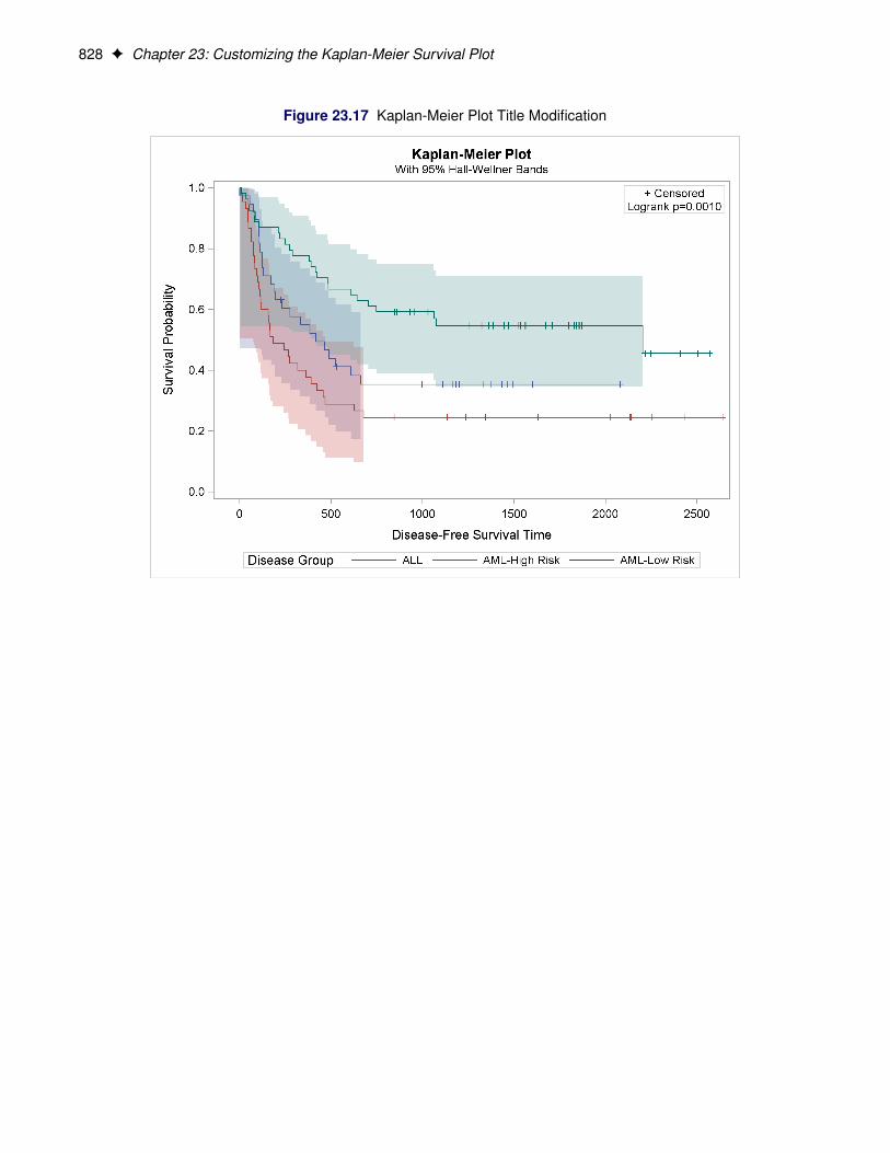
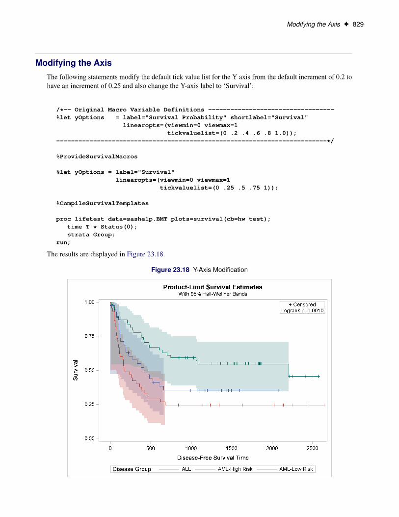
Modifying the AxisThe following statements modify the default tick value list for the Y axis from the default increment of 0.2 tohave an increment of 0.25 and also change the Y-axis label to ‘Survival’:
/*-- Original Macro Variable Definitions ----------------------------------%let yOptions = label="Survival Probability" shortlabel="Survival"
linearopts=(viewmin=0 viewmax=1tickvaluelist=(0 .2 .4 .6 .8 1.0));
-------------------------------------------------------------------------*/
%ProvideSurvivalMacros
%let yOptions = label="Survival"linearopts=(viewmin=0 viewmax=1
tickvaluelist=(0 .25 .5 .75 1));
%CompileSurvivalTemplates
proc lifetest data=sashelp.BMT plots=survival(cb=hw test);time T * Status(0);strata Group;
run;
The results are displayed in Figure 23.18.
Figure 23.18 Y-Axis Modification
830 F Chapter 23: Customizing the Kaplan-Meier Survival Plot
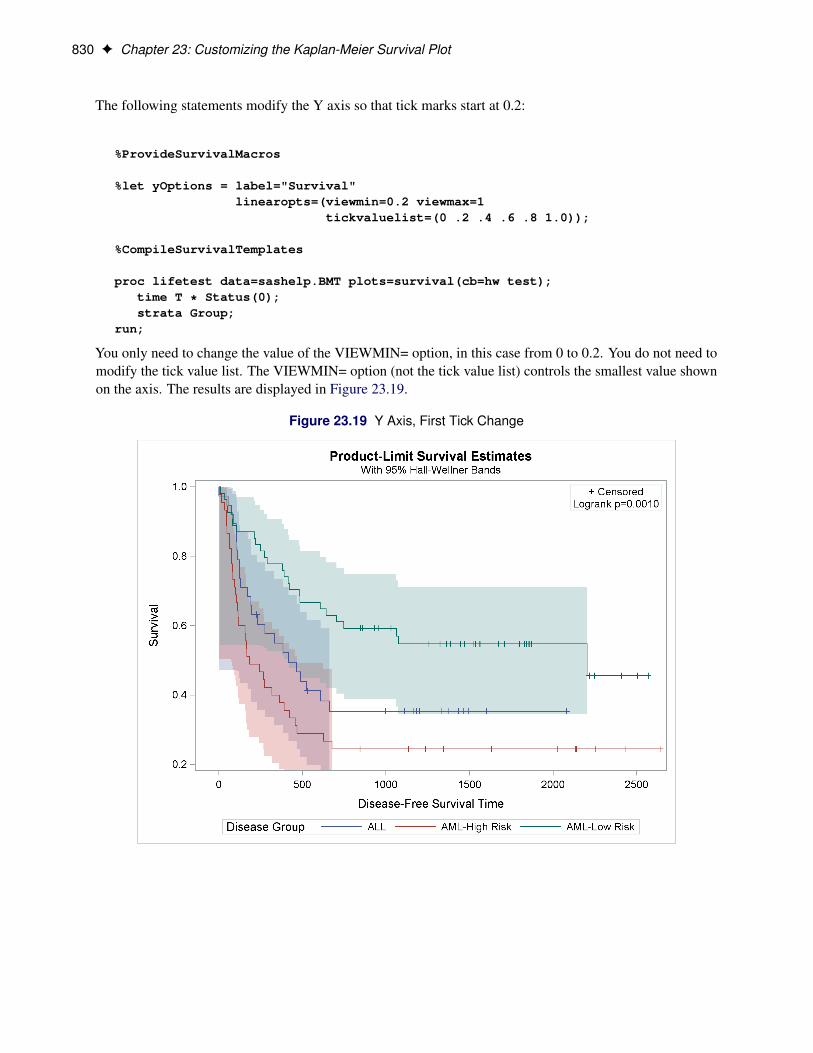
The following statements modify the Y axis so that tick marks start at 0.2:
%ProvideSurvivalMacros
%let yOptions = label="Survival"linearopts=(viewmin=0.2 viewmax=1
tickvaluelist=(0 .2 .4 .6 .8 1.0));
%CompileSurvivalTemplates
proc lifetest data=sashelp.BMT plots=survival(cb=hw test);time T * Status(0);strata Group;
run;
You only need to change the value of the VIEWMIN= option, in this case from 0 to 0.2. You do not need tomodify the tick value list. The VIEWMIN= option (not the tick value list) controls the smallest value shownon the axis. The results are displayed in Figure 23.19.
Figure 23.19 Y Axis, First Tick Change
Changing the Line Thickness F 831
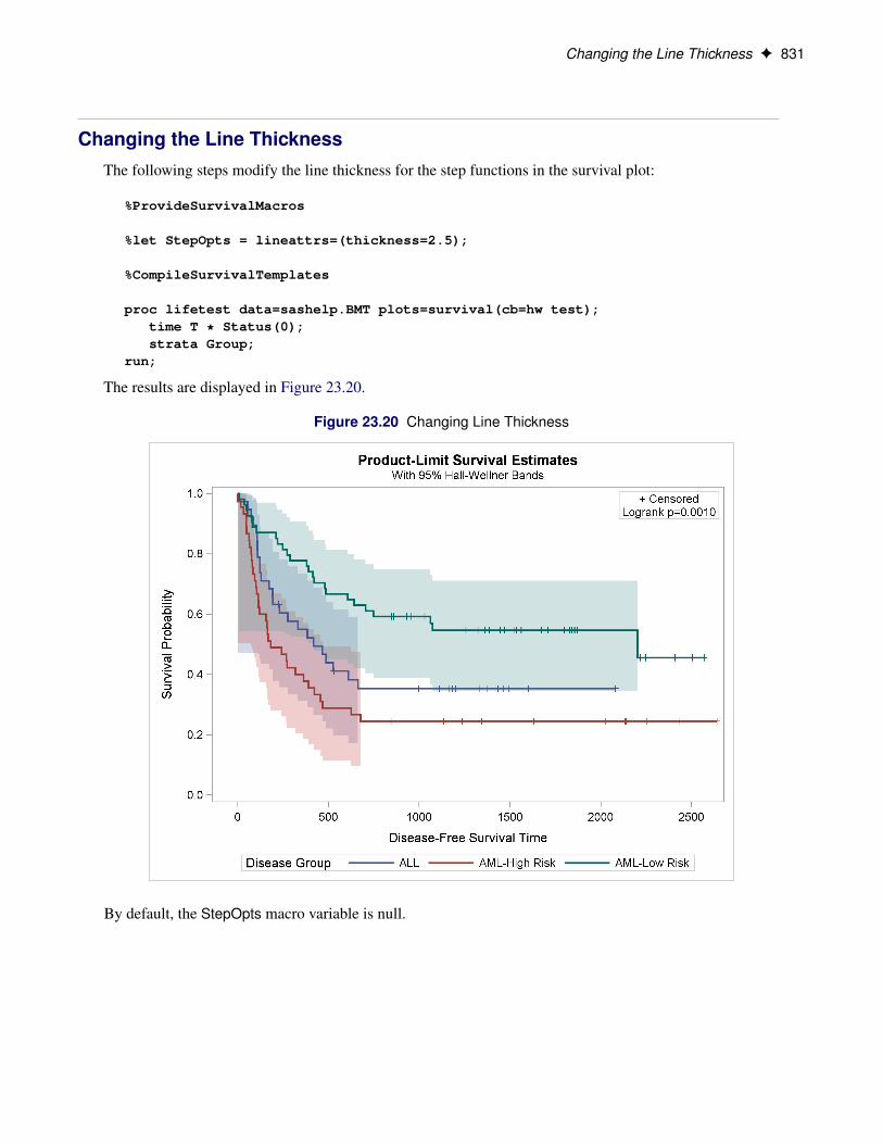
Changing the Line ThicknessThe following steps modify the line thickness for the step functions in the survival plot:
%ProvideSurvivalMacros
%let StepOpts = lineattrs=(thickness=2.5);
%CompileSurvivalTemplates
proc lifetest data=sashelp.BMT plots=survival(cb=hw test);time T * Status(0);strata Group;
run;
The results are displayed in Figure 23.20.
Figure 23.20 Changing Line Thickness
By default, the StepOpts macro variable is null.
832 F Chapter 23: Customizing the Kaplan-Meier Survival Plot
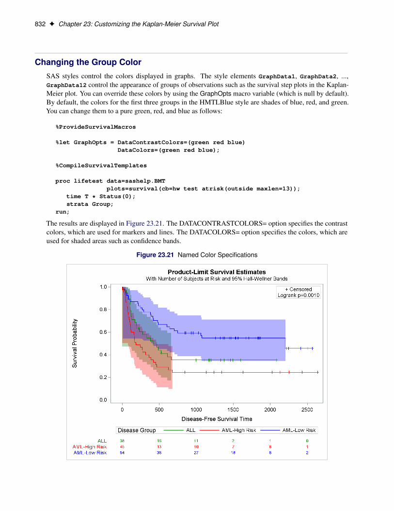
Changing the Group ColorSAS styles control the colors displayed in graphs. The style elements GraphData1, GraphData2, ...,GraphData12 control the appearance of groups of observations such as the survival step plots in the Kaplan-Meier plot. You can override these colors by using the GraphOpts macro variable (which is null by default).By default, the colors for the first three groups in the HMTLBlue style are shades of blue, red, and green.You can change them to a pure green, red, and blue as follows:
%ProvideSurvivalMacros
%let GraphOpts = DataContrastColors=(green red blue)DataColors=(green red blue);
%CompileSurvivalTemplates
proc lifetest data=sashelp.BMTplots=survival(cb=hw test atrisk(outside maxlen=13));
time T * Status(0);strata Group;
run;
The results are displayed in Figure 23.21. The DATACONTRASTCOLORS= option specifies the contrastcolors, which are used for markers and lines. The DATACOLORS= option specifies the colors, which areused for shaded areas such as confidence bands.
Figure 23.21 Named Color Specifications
Changing the Line Pattern F 833
The original colors (as shown in Figure 23.33) are more subtle than those shown in Figure 23.21. If you wantto change the order of the original colors by using this approach, then you need to know what they are so thatyou can specify them. The graph colors for the HTMLBlue and Statistical styles are extracted from the stylein the section “Displaying a Style and Extracting Color Lists” on page 868 and displayed in Figure 23.36.The section “Modifying Color Lists” on page 871 shows you how to change the graph template to specifythe original colors in a different order. The section “Swapping Colors among Style Elements” on page 872shows you how to use a macro to change a style template to specify the original colors in a different order(without having to extract and specify the color names).
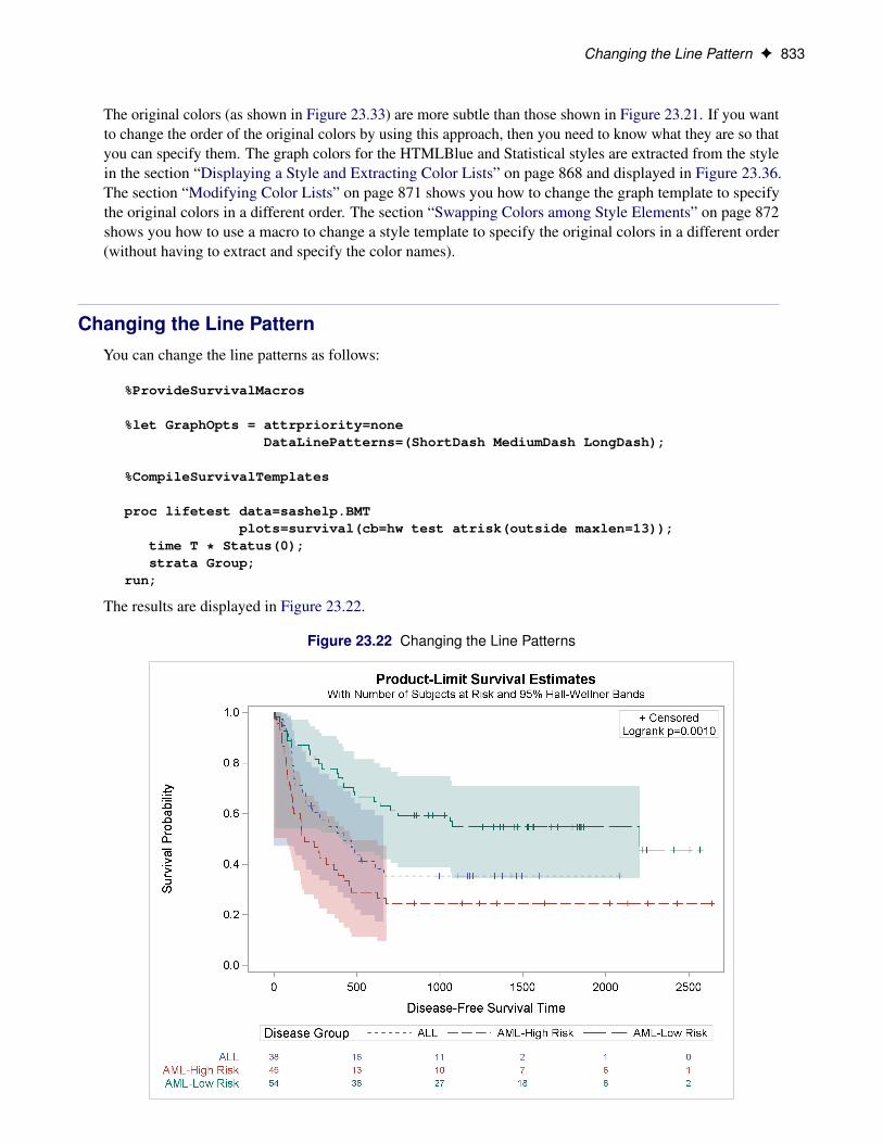
Changing the Line PatternYou can change the line patterns as follows:
%ProvideSurvivalMacros
%let GraphOpts = attrpriority=noneDataLinePatterns=(ShortDash MediumDash LongDash);
%CompileSurvivalTemplates
proc lifetest data=sashelp.BMTplots=survival(cb=hw test atrisk(outside maxlen=13));
time T * Status(0);strata Group;
run;
The results are displayed in Figure 23.22.
Figure 23.22 Changing the Line Patterns
834 F Chapter 23: Customizing the Kaplan-Meier Survival Plot
Other values for the DATALINEPATTERNS= option are provided in the section “The Macro Variables” onpage 853. You must use the option ATTRPRIORITY=NONE when you want to have varying line patterns inan ATTRPRIORITY=COLOR style like HTMLBlue or Pearl. In an ATTRPRIORITY=COLOR style, groupsare not distinguished by line patterns, and the line patterns for second and subsequent groups match the linepattern for the first group.
Changing the FontYou can change the Y-axis, X-axis, and title fonts as follows:
%ProvideSurvivalMacros
/*-- Original Macro Variable Definitions ----------------------------------%let TitleText0 = METHOD " Survival Estimate";%let TitleText1 = &titletext0 " for " STRATUMID;%let TitleText2 = &titletext0 "s";%let yOptions = label="Survival Probability"
shortlabel="Survival"linearopts=(viewmin=0 viewmax=1
tickvaluelist=(0 .2 .4 .6 .8 1.0));%let xOptions = shortlabel=XNAME
offsetmin=.05linearopts=(viewmax=MAXTIME tickvaluelist=XTICKVALS
tickvaluefitpolicy=XTICKVALFITPOL);-------------------------------------------------------------------------*/
%let tatters = textattrs=(size=12pt weight=bold family='arial');%let TitleText0 = METHOD " Survival Estimate";%let TitleText1 = &titletext0 " for " STRATUMID / &tatters;%let TitleText2 = &titletext0 "s" / &tatters;
%let yOptions = label="Survival Probability"shortlabel="Survival"labelattrs=(size=10pt weight=bold)tickvalueattrs=(size=8pt)linearopts=(viewmin=0 viewmax=1
tickvaluelist=(0 .2 .4 .6 .8 1.0));
%let xOptions = shortlabel=XNAMEoffsetmin=.05labelattrs=(size=10pt weight=bold)tickvalueattrs=(size=8pt)linearopts=(viewmax=MAXTIME tickvaluelist=XTICKVALS
tickvaluefitpolicy=XTICKVALFITPOL);
%CompileSurvivalTemplates
proc lifetest data=sashelp.BMT plots=survival(cb=hw test);time T * Status(0);strata Group;
run;
Changing the Font F 835
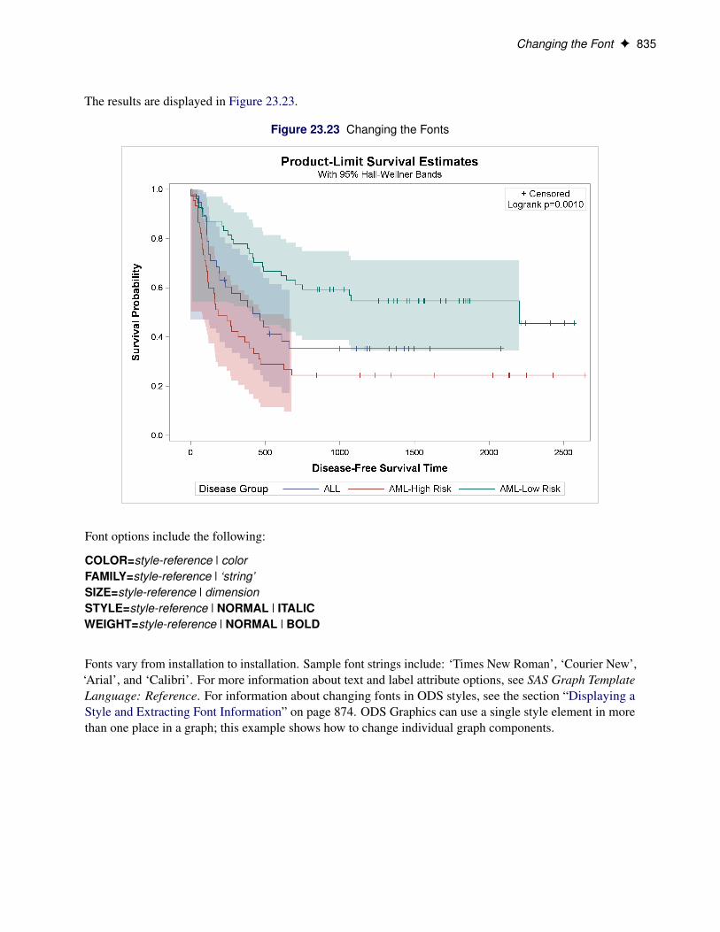
The results are displayed in Figure 23.23.
Figure 23.23 Changing the Fonts
Font options include the following:
COLOR=style-reference | colorFAMILY=style-reference | ‘string’SIZE=style-reference | dimensionSTYLE=style-reference | NORMAL | ITALICWEIGHT=style-reference | NORMAL | BOLD
Fonts vary from installation to installation. Sample font strings include: ‘Times New Roman’, ‘Courier New’,‘Arial’, and ‘Calibri’. For more information about text and label attribute options, see SAS Graph TemplateLanguage: Reference. For information about changing fonts in ODS styles, see the section “Displaying aStyle and Extracting Font Information” on page 874. ODS Graphics can use a single style element in morethan one place in a graph; this example shows how to change individual graph components.

836 F Chapter 23: Customizing the Kaplan-Meier Survival Plot
Changing the Legend and Inset PositionThis example shows you how to move the legend inside the plot (to the top right) and move the homogeneitytest and censored value legend to the bottom right of the plot:
%ProvideSurvivalMacros
/*-- Original Macro Variable Definitions ----------------------------------%let InsetOpts = autoalign=(TOPRIGHT BOTTOMLEFT TOP BOTTOM)
border=true BackgroundColor=GraphWalls:Color Opaque=true;%let LegendOpts = title=GROUPNAME location=outside;-------------------------------------------------------------------------*/
%let InsetOpts = autoalign=(BottomRight)border=true BackgroundColor=GraphWalls:Color Opaque=true;
%let LegendOpts = title=GROUPNAME location=inside across=1 autoalign=(TopRight);
%CompileSurvivalTemplates
proc lifetest data=sashelp.BMTplots=survival(cb=hw test atrisk(outside maxlen=13));
time T * Status(0);strata Group;
run;
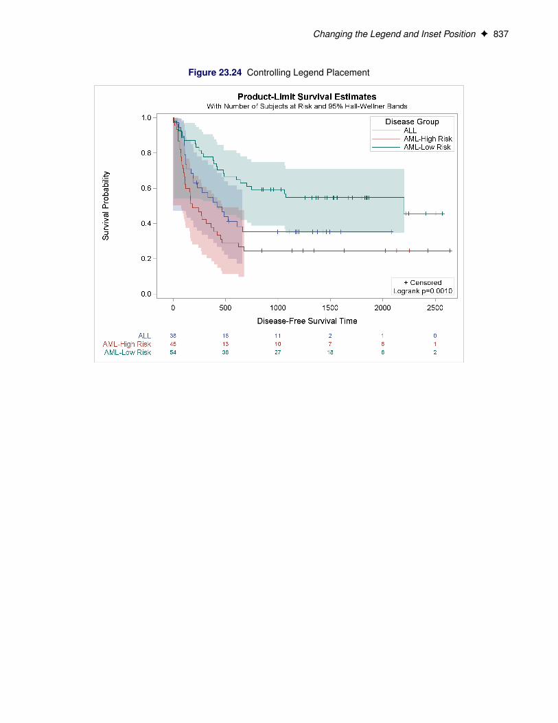
This example shows you how to replace the AUTOALIGN=(TOPRIGHT BOTTOMLEFT TOP BOT-TOM) option in the macro variable InsetOpts with AUTOALIGN=(BOTTOMRIGHT) and add the AU-TOALIGN=(TOPRIGHT) option to the LegendOpts macro variable. You can also add the option ACROSS=1to the LegendOpts macro variable to stack all legend entries vertically (with just one element in each row).
The results are displayed in Figure 23.24.
Changing the Legend and Inset Position F 837
Figure 23.24 Controlling Legend Placement
838 F Chapter 23: Customizing the Kaplan-Meier Survival Plot
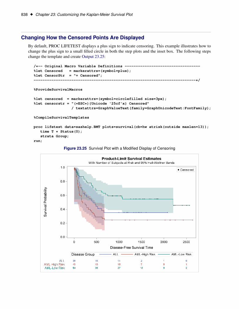
Changing How the Censored Points Are DisplayedBy default, PROC LIFETEST displays a plus sign to indicate censoring. This example illustrates how tochange the plus sign to a small filled circle in both the step plots and the inset box. The following stepschange the template and create Output 23.25:
/*-- Original Macro Variable Definitions ----------------------------------%let Censored = markerattrs=(symbol=plus);%let CensorStr = "+ Censored";-------------------------------------------------------------------------*/
%ProvideSurvivalMacros
%let censored = markerattrs=(symbol=circlefilled size=3px);%let censorstr = "(*ESC*){Unicode '25cf'x} Censored"
/ textattrs=GraphValueText(family=GraphUnicodeText:FontFamily);
%CompileSurvivalTemplates
proc lifetest data=sashelp.BMT plots=survival(cb=hw atrisk(outside maxlen=13));time T * Status(0);strata Group;
run;
Figure 23.25 Survival Plot with a Modified Display of Censoring
Adding a Y-Axis Reference Line F 839
The Unicode Consortium (http://unicode.org/) provides a list of character codes. Also see Fig-ure 22.2.7 in Chapter 22, “ODS Graphics Template Modification,” for information about the Unicodespecification for other markers. Although some Unicode characters are supported in some fonts, you shouldalways specify a Unicode font when using special characters.
Adding a Y-Axis Reference LineYou can add a horizontal reference line to the survival plot by adding the following statement to the template:
referenceline y=0.5;
You can do this by using the %StmtsTop macro. By default, this macro is empty. You can use the %StmtsTopmacro to add new statements to the beginning of the block of statements that define the appearance of thegraph. In contrast, you can use the %StmtsBottom macro to provide statements at the end of the statementblock. ODS Graphics draws statements in the order in which they appear; therefore, reference lines shouldbe drawn first so they do not obscure other parts of the graph.
The following step creates the plot in Figure 23.26:
%ProvideSurvivalMacros
%macro StmtsTop;referenceline y=0.5;
%mend;
%CompileSurvivalTemplates
proc lifetest data=sashelp.BMT plots=survival(cb=hw test);time T * Status(0);strata Group;
run;

840 F Chapter 23: Customizing the Kaplan-Meier Survival Plot
Figure 23.26 Horizontal Reference Line
Changing the Homogeneity Test Inset F 841
Changing the Homogeneity Test InsetThis example modifies the contents of the %pValue macro. The original %pValue macro definition is asfollows:
%macro pValue;if (PVALUE < .0001)
entry TESTNAME " p " eval (PUT(PVALUE, PVALUE6.4));else
entry TESTNAME " p=" eval (PUT(PVALUE, PVALUE6.4));endif;
%mend;
The following example directly specifies the test name (replacing the internal name ‘Logrank’ with ‘LogRank’) and adds blank spaces around the equal sign:
%ProvideSurvivalMacros
%macro pValue;if (PVALUE < .0001)
entry "Log Rank p " eval (PUT(PVALUE, PVALUE6.4));else
entry "Log Rank p = " eval (PUT(PVALUE, PVALUE6.4));endif;
%mend;
%CompileSurvivalTemplates
proc lifetest data=sashelp.BMT plots=survival(cb=hw test);time T * Status(0);strata Group;
run;
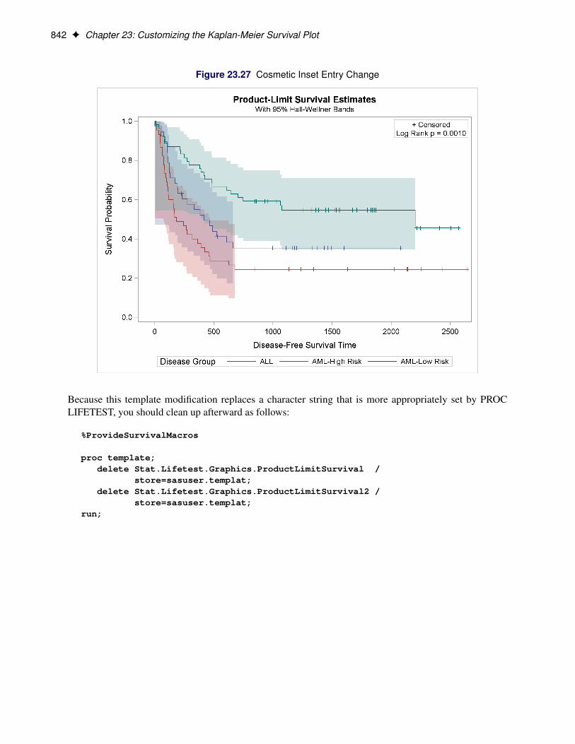
The results are displayed in Figure 23.27.
842 F Chapter 23: Customizing the Kaplan-Meier Survival Plot
Figure 23.27 Cosmetic Inset Entry Change
Because this template modification replaces a character string that is more appropriately set by PROCLIFETEST, you should clean up afterward as follows:
%ProvideSurvivalMacros
proc template;delete Stat.Lifetest.Graphics.ProductLimitSurvival /
store=sasuser.templat;delete Stat.Lifetest.Graphics.ProductLimitSurvival2 /
store=sasuser.templat;run;
Suppressing the Second Title and Adding a Footnote F 843
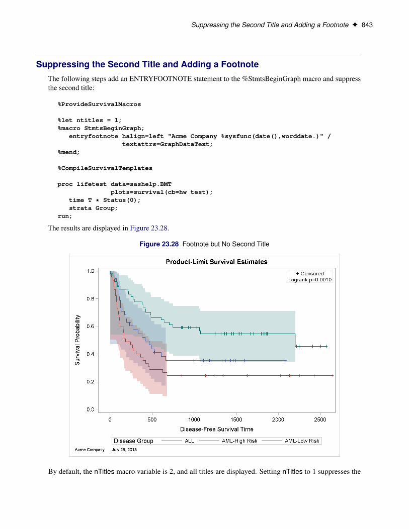
Suppressing the Second Title and Adding a FootnoteThe following steps add an ENTRYFOOTNOTE statement to the %StmtsBeginGraph macro and suppressthe second title:
%ProvideSurvivalMacros
%let ntitles = 1;%macro StmtsBeginGraph;
entryfootnote halign=left "Acme Company %sysfunc(date(),worddate.)" /textattrs=GraphDataText;
%mend;
%CompileSurvivalTemplates
proc lifetest data=sashelp.BMTplots=survival(cb=hw test);
time T * Status(0);strata Group;
run;
The results are displayed in Figure 23.28.
Figure 23.28 Footnote but No Second Title
By default, the nTitles macro variable is 2, and all titles are displayed. Setting nTitles to 1 suppresses the
844 F Chapter 23: Customizing the Kaplan-Meier Survival Plot
second title. You can add titles or footnotes to the plot by adding them to the %StmtsBeginGraph macro.This example adds a footnote that consists of a company name followed by the current date, formatted byusing the WORDDATE format. The GraphDataText style element is used; it has a smaller font than thedefault style element, GraphFootnoteText.
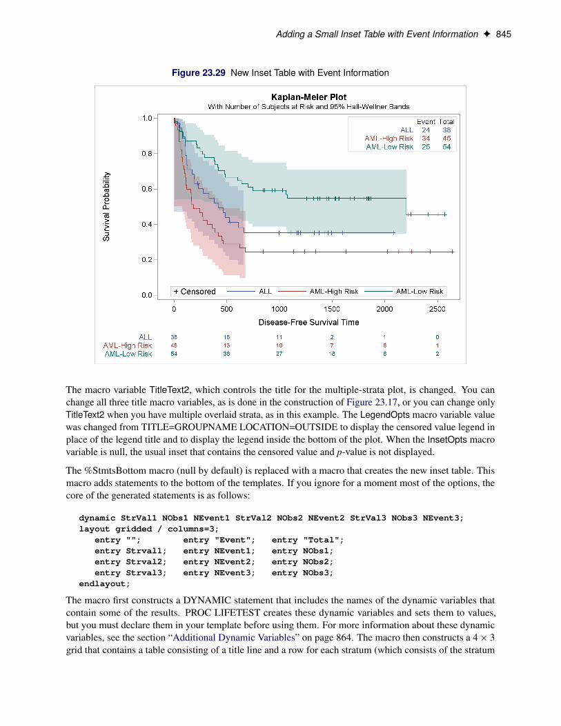
Adding a Small Inset Table with Event InformationThis example shows you how to modify the template to produce the plot displayed in Output 23.29. This newplot has an inset table in the top right corner that shows the number of observations and the number of eventsin each stratum. The legend has been moved inside the plot and combined with the old inset table that showsthe marker for censored observations.6 Also, the title is changed to ‘Kaplan-Meier Plot’.
%ProvideSurvivalMacros
%let TitleText2 = "Kaplan-Meier Plot";%let LegendOpts = title="+ Censored"
location=inside autoalign=(Bottom);%let InsetOpts = ;
%macro StmtsBottom;dynamic %do i = 1 %to 3; StrVal&i NObs&i NEvent&i %end;;layout gridded / columns=3 border=TRUE autoalign=(TopRight);
entry ""; entry "Event"; entry "Total";%do i = 1 %to 3;
%let t = / textattrs=GraphData&i;entry halign=right Strval&i &t; entry NEvent&i &t; entry NObs&i &t;
%end;endlayout;
%mend;
%CompileSurvivalTemplates
proc lifetest data=sashelp.BMT plots=survival(cb=hw atrisk(outside maxlen=13));time T * Status(0);strata Group;
run;
The results are displayed in Figure 23.29.
6This legend is wide and might not be displayed if your graph is small. If the legend is not displayed, try increasing the size ofthe graph by specifying the WIDTH= or HEIGHT= option in the ODS GRAPHICS statement.
Adding a Small Inset Table with Event Information F 845
Figure 23.29 New Inset Table with Event Information
The macro variable TitleText2, which controls the title for the multiple-strata plot, is changed. You canchange all three title macro variables, as is done in the construction of Figure 23.17, or you can change onlyTitleText2 when you have multiple overlaid strata, as in this example. The LegendOpts macro variable valuewas changed from TITLE=GROUPNAME LOCATION=OUTSIDE to display the censored value legend inplace of the legend title and to display the legend inside the bottom of the plot. When the InsetOpts macrovariable is null, the usual inset that contains the censored value and p-value is not displayed.
The %StmtsBottom macro (null by default) is replaced with a macro that creates the new inset table. Thismacro adds statements to the bottom of the templates. If you ignore for a moment most of the options, thecore of the generated statements is as follows:
dynamic StrVal1 NObs1 NEvent1 StrVal2 NObs2 NEvent2 StrVal3 NObs3 NEvent3;layout gridded / columns=3;
entry ""; entry "Event"; entry "Total";entry Strval1; entry NEvent1; entry NObs1;entry Strval2; entry NEvent2; entry NObs2;entry Strval3; entry NEvent3; entry NObs3;
endlayout;
The macro first constructs a DYNAMIC statement that includes the names of the dynamic variables thatcontain some of the results. PROC LIFETEST creates these dynamic variables and sets them to values,but you must declare them in your template before using them. For more information about these dynamicvariables, see the section “Additional Dynamic Variables” on page 864. The macro then constructs a 4 � 3grid that contains a table consisting of a title line and a row for each stratum (which consists of the stratum
846 F Chapter 23: Customizing the Kaplan-Meier Survival Plot
label, the number of events, and the total number of subjects). The full layout that the %StmtsBottom macrogenerates, with all the options, is as follows:
dynamic StrVal1 NObs1 NEvent1 StrVal2 NObs2 NEvent2 StrVal3 NObs3 NEvent3;layout gridded / columns=3 border=TRUE autoalign=(TopRight);
entry "";entry "Event";entry "Total";entry halign=right Strval1 / textattrs=GraphData1;entry NEvent1 / textattrs=GraphData1;entry NObs1 / textattrs=GraphData1;entry halign=right Strval2 / textattrs=GraphData2;entry NEvent2 / textattrs=GraphData2;entry NObs2 / textattrs=GraphData2;entry halign=right Strval3 / textattrs=GraphData3;entry NEvent3 / textattrs=GraphData3;entry NObs3 / textattrs=GraphData3;
endlayout;
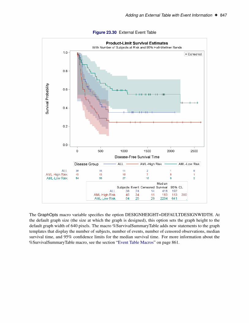
Adding an External Table with Event InformationThis example adds a table to the plot that displays a summary of event information. The following statementscreate Figure 23.30:
%ProvideSurvivalMacros
%let GraphOpts = DesignHeight=DefaultDesignWidth;
%SurvivalSummaryTable
%CompileSurvivalTemplates
proc lifetest data=sashelp.BMTplots=survival(cb=hw atrisk(outside maxlen=13));
time T * Status(0);strata Group;
run;
Adding an External Table with Event Information F 847
Figure 23.30 External Event Table
The GraphOpts macro variable specifies the option DESIGNHEIGHT=DEFAULTDESIGNWIDTH. Atthe default graph size (the size at which the graph is designed), this option sets the graph height to thedefault graph width of 640 pixels. The macro %SurvivalSummaryTable adds new statements to the graphtemplates that display the number of subjects, number of events, number of censored observations, mediansurvival time, and 95% confidence limits for the median survival time. For more information about the%SurvivalSummaryTable macro, see the section “Event Table Macros” on page 861.
848 F Chapter 23: Customizing the Kaplan-Meier Survival Plot
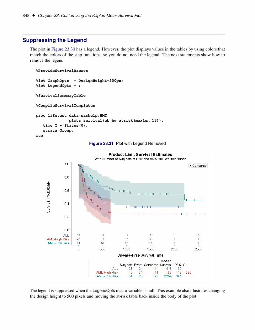
Suppressing the LegendThe plot in Figure 23.30 has a legend. However, the plot displays values in the tables by using colors thatmatch the colors of the step functions, so you do not need the legend. The next statements show how toremove the legend:
%ProvideSurvivalMacros
%let GraphOpts = DesignHeight=500px;%let LegendOpts = ;
%SurvivalSummaryTable
%CompileSurvivalTemplates
proc lifetest data=sashelp.BMTplots=survival(cb=hw atrisk(maxlen=13));
time T * Status(0);strata Group;
run;
Figure 23.31 Plot with Legend Removed
The legend is suppressed when the LegendOpts macro variable is null. This example also illustrates changingthe design height to 500 pixels and moving the at-risk table back inside the body of the plot.
Kaplan-Meier Plot with Event Table and Other Customizations F 849
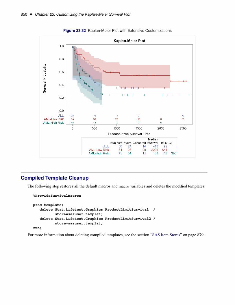
Kaplan-Meier Plot with Event Table and Other CustomizationsThis example combines a number of features from previous examples. The order of the strata levels in thetables is ALL, AML–Low Risk, and AML–High Risk (see the section “Reordering the Groups” on page 820).The title is set to ‘Kaplan-Meier Plot’ (see the section “Changing the Plot Title” on page 827). The secondtitle line is suppressed (see the section “Suppressing the Second Title and Adding a Footnote” on page 843).The graph height is set to 500 pixels (see the section “Suppressing the Legend” on page 848). The legend andthe inset box that contains the legend for censored values are both suppressed (see the sections “Suppressingthe Legend” on page 848 and “Adding a Small Inset Table with Event Information” on page 844). The eventtable is displayed outside the plot (see the section “Adding an External Table with Event Information” onpage 846) and the at-risk table is displayed inside the plot (see the section “Displaying the Patients-at-RiskTable inside the Plot” on page 814).
proc format;invalue bmtnum 'ALL' = 1 'AML-Low Risk' = 2 'AML-High Risk' = 3;value bmtfmt 1 = 'ALL' 2 = 'AML-Low Risk' 3 = 'AML-High Risk';
run;
data BMT(drop=g);set sashelp.BMT(rename=(group=g));Group = input(g, bmtnum.);
run;
%ProvideSurvivalMacros
%let TitleText2 = "Kaplan-Meier Plot";%let nTitles = 1;%let GraphOpts = DesignHeight=500px;%let LegendOpts = ;%let InsetOpts = ;
%SurvivalSummaryTable
%CompileSurvivalTemplates
proc lifetest data=BMT plots=survival(cb=hw atrisk(maxlen=13));time T * Status(0);strata Group / order=internal;format group bmtfmt.;
run;
The results are displayed in Figure 23.32.
850 F Chapter 23: Customizing the Kaplan-Meier Survival Plot
Figure 23.32 Kaplan-Meier Plot with Extensive Customizations
Compiled Template CleanupThe following step restores all the default macros and macro variables and deletes the modified templates:
%ProvideSurvivalMacros
proc template;delete Stat.Lifetest.Graphics.ProductLimitSurvival /
store=sasuser.templat;delete Stat.Lifetest.Graphics.ProductLimitSurvival2 /
store=sasuser.templat;run;
For more information about deleting compiled templates, see the section “SAS Item Stores” on page 879.
Graph Templates, Macros, and Macro Variables F 851
Graph Templates, Macros, and Macro VariablesThe %ProvideSurvivalMacros macro and the macros and macro variables that it provides have the followingproperties:
� Many options, including most of the options that are specified in multiple places in the templates, areextracted to macro variables.
� The %CompileSurvivalTemplates macro provides the main body of the two templates. You can call itto compile the templates after making changes.
- The template Stat.Lifetest.Graphics.ProductLimitSurvival provides the survival tem-plate when the at-risk table is inside the body of the plot.
- The template Stat.Lifetest.Graphics.ProductLimitSurvival2 provides the survivaltemplate when the at-risk table is outside the body of the plot.7
The two templates share many statements, and a macro %DO loop creates both versions.
� The portion of the templates for the table for the p-values is stored in the macro %pValue.
� The portion of the templates for the single-stratum case is stored in the macro %SingleStratum.
� The portion of the templates for the multiple-strata case is stored in the macro %MultipleStrata.
� The macro %AtRiskLatticeStart begins the two-cell lattice that contains the plot above the table whenthe at-risk table is outside the body of the plot.
� The macro %AtRiskLatticeEnd ends the two-cell lattice that contains the plot and the table when theat-risk table is outside the body of the plot.
� Some empty macros (%StmtsBeginGraph, %StmtsTop, and %StmtsBottom) are provided to enableyou to add statements and options to strategic places in the templates.
� The %SurvTabHeader, %SurvivalTable, and %SurvivalSummaryTable macros enable you to easilyadd more GTL statements to the Kaplan-Meier plot templates to display event information for eachstratum.
7The macros do not affect any graph that uses graph templates other than the two templates that are modified here. The macrosdo not affect the STRATA=PANEL plot that uses the templateStat.Lifetest.Graphics.ProductLimitSurvivalPanelor the failure plot that uses the template Stat.Lifetest.Graphics.ProductLimitFailure.
852 F Chapter 23: Customizing the Kaplan-Meier Survival Plot
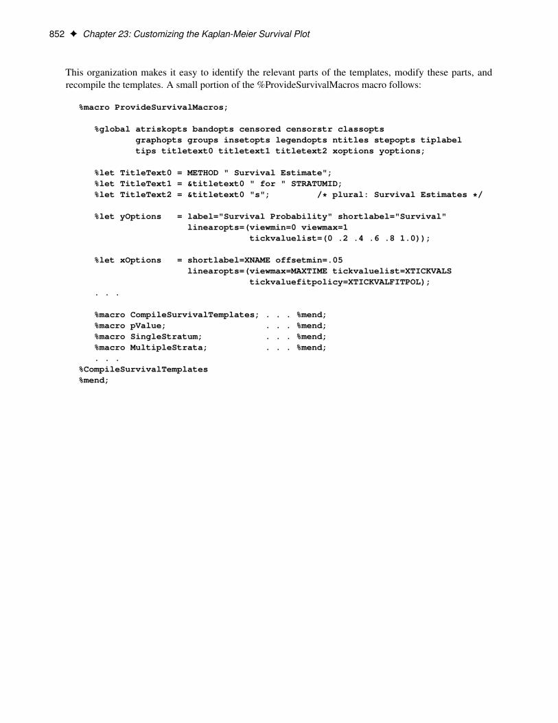
This organization makes it easy to identify the relevant parts of the templates, modify these parts, andrecompile the templates. A small portion of the %ProvideSurvivalMacros macro follows:
%macro ProvideSurvivalMacros;
%global atriskopts bandopts censored censorstr classoptsgraphopts groups insetopts legendopts ntitles stepopts tiplabeltips titletext0 titletext1 titletext2 xoptions yoptions;
%let TitleText0 = METHOD " Survival Estimate";%let TitleText1 = &titletext0 " for " STRATUMID;%let TitleText2 = &titletext0 "s"; /* plural: Survival Estimates */
%let yOptions = label="Survival Probability" shortlabel="Survival"linearopts=(viewmin=0 viewmax=1
tickvaluelist=(0 .2 .4 .6 .8 1.0));
%let xOptions = shortlabel=XNAME offsetmin=.05linearopts=(viewmax=MAXTIME tickvaluelist=XTICKVALS
tickvaluefitpolicy=XTICKVALFITPOL);. . .
%macro CompileSurvivalTemplates; . . . %mend;%macro pValue; . . . %mend;%macro SingleStratum; . . . %mend;%macro MultipleStrata; . . . %mend;. . .
%CompileSurvivalTemplates%mend;
The Macro Variables F 853
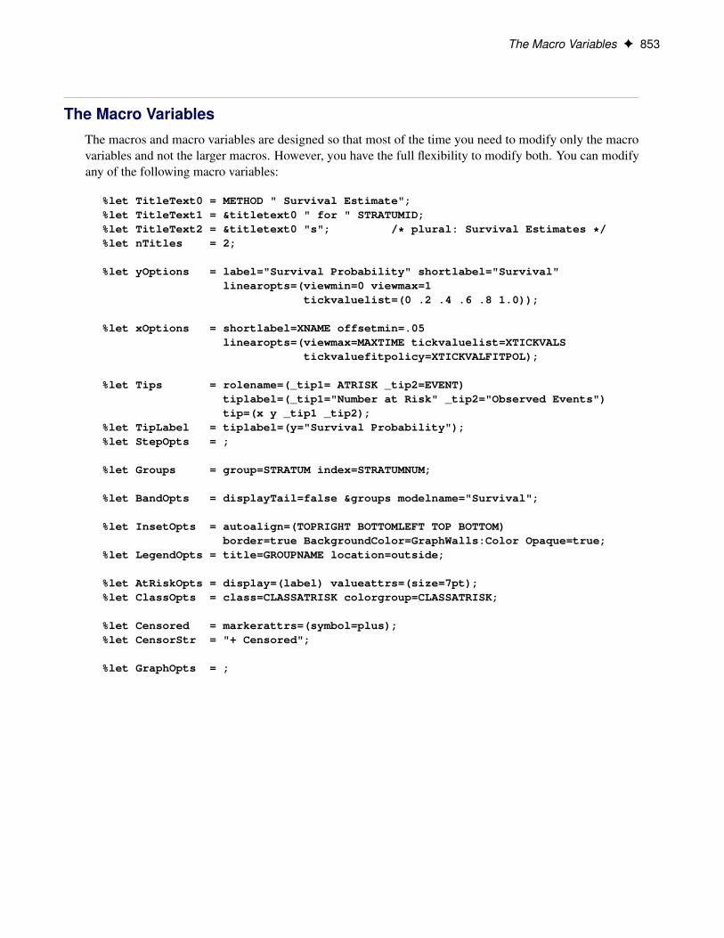
The Macro VariablesThe macros and macro variables are designed so that most of the time you need to modify only the macrovariables and not the larger macros. However, you have the full flexibility to modify both. You can modifyany of the following macro variables:
%let TitleText0 = METHOD " Survival Estimate";%let TitleText1 = &titletext0 " for " STRATUMID;%let TitleText2 = &titletext0 "s"; /* plural: Survival Estimates */%let nTitles = 2;
%let yOptions = label="Survival Probability" shortlabel="Survival"linearopts=(viewmin=0 viewmax=1
tickvaluelist=(0 .2 .4 .6 .8 1.0));
%let xOptions = shortlabel=XNAME offsetmin=.05linearopts=(viewmax=MAXTIME tickvaluelist=XTICKVALS
tickvaluefitpolicy=XTICKVALFITPOL);
%let Tips = rolename=(_tip1= ATRISK _tip2=EVENT)tiplabel=(_tip1="Number at Risk" _tip2="Observed Events")tip=(x y _tip1 _tip2);
%let TipLabel = tiplabel=(y="Survival Probability");%let StepOpts = ;
%let Groups = group=STRATUM index=STRATUMNUM;
%let BandOpts = displayTail=false &groups modelname="Survival";
%let InsetOpts = autoalign=(TOPRIGHT BOTTOMLEFT TOP BOTTOM)border=true BackgroundColor=GraphWalls:Color Opaque=true;
%let LegendOpts = title=GROUPNAME location=outside;
%let AtRiskOpts = display=(label) valueattrs=(size=7pt);%let ClassOpts = class=CLASSATRISK colorgroup=CLASSATRISK;
%let Censored = markerattrs=(symbol=plus);%let CensorStr = "+ Censored";
%let GraphOpts = ;
854 F Chapter 23: Customizing the Kaplan-Meier Survival Plot
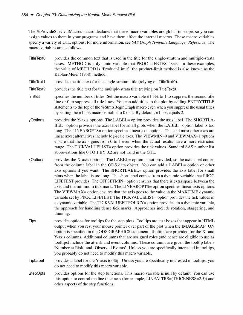
The %ProvideSurvivalMacros macro declares that these macro variables are global in scope, so you canassign values to them in your programs and have them affect the internal macros. These macro variablesspecify a variety of GTL options; for more information, see SAS Graph Template Language: Reference. Themacro variables are as follows.
TitleText0 provides the common text that is used in the title for the single-stratum and multiple-stratacases. METHOD is a dynamic variable that PROC LIFETEST sets. In these examples,the value of METHOD is ‘Product-Limit’; the product-limit method is also known as theKaplan-Meier (1958) method.
TitleText1 provides the title text for the single-stratum title (relying on TitleText0).
TitleText2 provides the title text for the multiple-strata title (relying on TitleText0).
nTitles specifies the number of titles. Set the macro variable nTitles to 1 to suppress the second titleline or 0 to suppress all title lines. You can add titles to the plot by adding ENTRYTITLEstatements to the top of the %StmtsBeginGraph macro even when you suppress the usual titlesby setting the nTitles macro variable to 0 or 1. By default, nTitles equals 2.
yOptions provides the Y-axis options. The LABEL= option provides the axis label. The SHORTLA-BEL= option provides the axis label for small plots when the LABEL= option label is toolong. The LINEAROPTS= option specifies linear axis options. This and most other axes arelinear axes; alternatives include log-scale axes. The VIEWMIN=0 and VIEWMAX=1 optionsensure that the axis goes from 0 to 1 even when the actual results have a more restrictedrange. The TICKVALUELIST= option provides the tick values. Standard SAS number listabbreviations like 0 TO 1 BY 0.2 are not valid in the GTL.
xOptions provides the X-axis options. The LABEL= option is not provided, so the axis label comesfrom the column label in the ODS data object. You can add a LABEL= option or otheraxis options if you want. The SHORTLABEL= option provides the axis label for smallplots when the label is too long. The short label comes from a dynamic variable that PROCLIFETEST provides. The OFFSETMIN= option ensures that there is extra space between theaxis and the minimum tick mark. The LINEAROPTS= option specifies linear axis options.The VIEWMAX= option ensures that the axis goes to the value in the MAXTIME dynamicvariable set by PROC LIFETEST. The TICKVALUELIST= option provides the tick values ina dynamic variable. The TICKVALUEFITPOLICY= option provides, in a dynamic variable,the approach for handling dense tick marks. Approaches include rotation, staggering, andthinning.
Tips provides options for tooltips for the step plots. Tooltips are text boxes that appear in HTMLoutput when you rest your mouse pointer over part of the plot when the IMAGEMAP=ONoption is specified in the ODS GRAPHICS statement. Tooltips are provided for the X- andY-axis columns. Additional columns that are assigned roles (and hence are eligible to use astooltips) include the at-risk and event columns. These columns are given the tooltip labels‘Number at Risk’ and ‘Observed Events’. Unless you are specifically interested in tooltips,you probably do not need to modify this macro variable.
TipLabel provides a label for the Y-axis tooltip. Unless you are specifically interested in tooltips, youdo not need to modify this macro variable.
StepOpts provides options for the step functions. This macro variable is null by default. You can usethis option to control the line thickness (for example, LINEATTRS=(THICKNESS=2.5)) andother aspects of the step functions.
The Macro Variables F 855
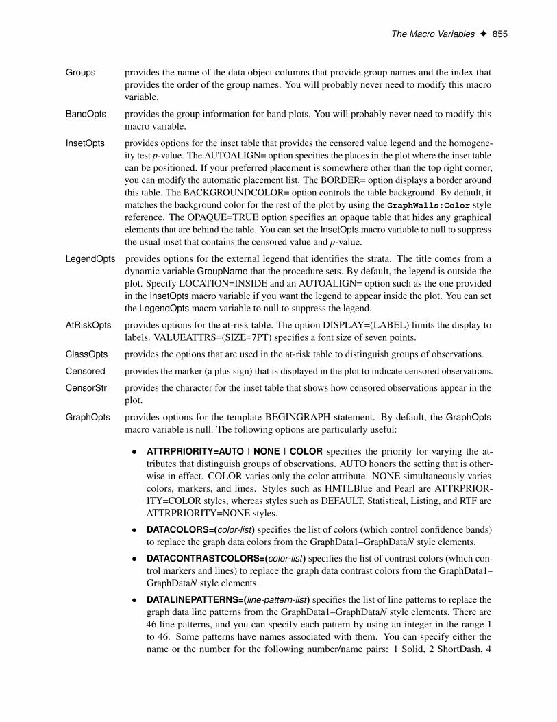
Groups provides the name of the data object columns that provide group names and the index thatprovides the order of the group names. You will probably never need to modify this macrovariable.
BandOpts provides the group information for band plots. You will probably never need to modify thismacro variable.
InsetOpts provides options for the inset table that provides the censored value legend and the homogene-ity test p-value. The AUTOALIGN= option specifies the places in the plot where the inset tablecan be positioned. If your preferred placement is somewhere other than the top right corner,you can modify the automatic placement list. The BORDER= option displays a border aroundthis table. The BACKGROUNDCOLOR= option controls the table background. By default, itmatches the background color for the rest of the plot by using the GraphWalls:Color stylereference. The OPAQUE=TRUE option specifies an opaque table that hides any graphicalelements that are behind the table. You can set the InsetOpts macro variable to null to suppressthe usual inset that contains the censored value and p-value.
LegendOpts provides options for the external legend that identifies the strata. The title comes from adynamic variable GroupName that the procedure sets. By default, the legend is outside theplot. Specify LOCATION=INSIDE and an AUTOALIGN= option such as the one providedin the InsetOpts macro variable if you want the legend to appear inside the plot. You can setthe LegendOpts macro variable to null to suppress the legend.
AtRiskOpts provides options for the at-risk table. The option DISPLAY=(LABEL) limits the display tolabels. VALUEATTRS=(SIZE=7PT) specifies a font size of seven points.
ClassOpts provides the options that are used in the at-risk table to distinguish groups of observations.
Censored provides the marker (a plus sign) that is displayed in the plot to indicate censored observations.
CensorStr provides the character for the inset table that shows how censored observations appear in theplot.
GraphOpts provides options for the template BEGINGRAPH statement. By default, the GraphOptsmacro variable is null. The following options are particularly useful:
� ATTRPRIORITY=AUTO | NONE | COLOR specifies the priority for varying the at-tributes that distinguish groups of observations. AUTO honors the setting that is other-wise in effect. COLOR varies only the color attribute. NONE simultaneously variescolors, markers, and lines. Styles such as HMTLBlue and Pearl are ATTRPRIOR-ITY=COLOR styles, whereas styles such as DEFAULT, Statistical, Listing, and RTF areATTRPRIORITY=NONE styles.
� DATACOLORS=(color-list) specifies the list of colors (which control confidence bands)to replace the graph data colors from the GraphData1–GraphDataN style elements.
� DATACONTRASTCOLORS=(color-list) specifies the list of contrast colors (which con-trol markers and lines) to replace the graph data contrast colors from the GraphData1–GraphDataN style elements.
� DATALINEPATTERNS=(line-pattern-list) specifies the list of line patterns to replace thegraph data line patterns from the GraphData1–GraphDataN style elements. There are46 line patterns, and you can specify each pattern by using an integer in the range 1to 46. Some patterns have names associated with them. You can specify either thename or the number for the following number/name pairs: 1 Solid, 2 ShortDash, 4
856 F Chapter 23: Customizing the Kaplan-Meier Survival Plot
MediumDash, 5 LongDash, 8 MediumDashShortDash, 14 DashDashDot, 15 DashDot-Dot, 20 Dash, 26 LongDashShortDash, 34 Dot, 35 ThinDot, 41 ShortDashDot, and 42MediumDashDotDot.
� DESIGNHEIGHT=height sets the graph height. You can set the graph heightto the default graph width of 640 pixels by specifying the option DESIGN-HEIGHT=DEFAULTDESIGNWIDTH. Or you can specify a size in pixels, such asDESIGNHEIGHT=500PX. Although the graph is designed at the specified height, youcan resize it for the actual display by using the WIDTH= and HEIGHT= options in theODS GRAPHICS statement. By default, DESIGNHEIGHT=480PX.
� DESIGNWIDTH=width sets the graph width. You can set the graph widthto the default graph height of 480 pixels by specifying the option DESIGN-WIDTH=DEFAULTDESIGNHEIGHT. Or you can specify a size in pixels, suchas DESIGNWIDTH=600PX. Although the graph is designed at the specified width, youcan resize it for the actual display by using the WIDTH= and HEIGHT= options in theODS GRAPHICS statement. By default, DESIGNWIDTH=640PX.
The Smaller MacrosThe %ProvideSurvivalMacros macro provides four small macros that are easy for you to modify:
%macro StmtsBeginGraph; %mend;%macro StmtsTop; %mend;%macro StmtsBottom; %mend;
%macro pValue;if (PVALUE < .0001)
entry TESTNAME " p " eval (PUT(PVALUE, PVALUE6.4));else
entry TESTNAME " p=" eval (PUT(PVALUE, PVALUE6.4));endif;
%mend;
By default, the %StmtsBeginGraph, %StmtsTop, and %StmtsBottom macros are empty. You can use them toadd new statements to the BEGINGRAPH block or to the beginning or end of the block of statements thatdefine the appearance of the graph.
The %pValue macro is used to control the display of the p-value from the homogeneity test.
The Larger MacrosThe examples and information up to this point have illustrated how you can make simple changes to thesurvival plot. It is unlikely that you will ever have to do more than that. If you need to make changes to theoverall layout of the graph, then you must modify one of the other macros. The %CompileSurvivalTemplatesmacro, which is the macro that compiles all the pieces that you modified, is as follows:
The Larger Macros F 857
%macro CompileSurvivalTemplates;%local outside;proc template;
%do outside = 0 %to 1;define statgraph
Stat.Lifetest.Graphics.ProductLimitSurvival%scan(2,2-&outside);dynamic NStrata xName plotAtRisk
%if %nrbquote(&censored) ne %then plotCensored;plotCL plotHW plotEP labelCL labelHW labelEP maxTime xtickValsxtickValFitPol rowWeights method StratumID classAtRiskplotTest GroupName Transparency SecondTitle TestName pValue_byline_ _bytitle_ _byfootnote_;
BeginGraph %if %nrbquote(&graphopts) ne %then / &graphopts;;
if (NSTRATA=1)%if &ntitles %then %do;
if (EXISTS(STRATUMID)) entrytitle &titletext1;else entrytitle &titletext0;endif;
%end;
%if &ntitles gt 1 %then %do;%if not &outside %then if (PLOTATRISK=1);
entrytitle "With Number of Subjects at Risk" /textattrs=GRAPHVALUETEXT;
%if not &outside %then %do; endif; %end;%end;
%StmtsBeginGraph%AtRiskLatticeStartlayout overlay / xaxisopts=(&xoptions) yaxisopts=(&yoptions);
%StmtsTop%SingleStratum%StmtsBottom
endlayout;%AtRiskLatticeEnd
else%if &ntitles %then %do; entrytitle &titletext2; %end;%if &ntitles gt 1 %then %do;
if (EXISTS(SECONDTITLE))entrytitle SECONDTITLE / textattrs=GRAPHVALUETEXT;
endif;%end;
%StmtsBeginGraph%AtRiskLatticeStartlayout overlay / xaxisopts=(&xoptions) yaxisopts=(&yoptions);
%StmtsTop%MultipleStrata%StmtsBottom
endlayout;%AtRiskLatticeEnd(class)
endif;
858 F Chapter 23: Customizing the Kaplan-Meier Survival Plot
if (_BYTITLE_) entrytitle _BYLINE_ / textattrs=GRAPHVALUETEXT;else if (_BYFOOTNOTE_) entryfootnote halign=left _BYLINE_; endif;endif;EndGraph;
end;%end;
run;%mend;
The macro %DO loop compiles the following two templates:
� Stat.Lifetest.Graphics.ProductLimitSurvival when the macro variable Outside is 0 and%SCAN(2,2-&OUTSIDE) is null
� Stat.Lifetest.Graphics.ProductLimitSurvival2 when the macro variable Outside is 1 and%SCAN(2,2-&OUTSIDE) is 2
The primary difference between these templates is that when the macro variable Outside is 1, a LAYOUTLATTICE statement block is used to place the at-risk table outside the graph. When Outside is 1, the macros%AtRiskLatticeStart and %AtRiskLatticeEnd provide the LAYOUT LATTICE statement block (two cells,plot above and at-risk table below) and the LAYOUT OVERLAY statement block for the at-risk table. The%AtRiskLatticeStart and %AtRiskLatticeEnd macros are defined as follows:
%macro AtRiskLatticeStart;%if &outside %then %do;
layout lattice / rows=2 rowweights=ROWWEIGHTScolumndatarange=union rowgutter=10;
cell;%end;
%mend;
%macro AtRiskLatticeEnd(useclassopts);%if &outside %then %do;
endcell;cell;
layout overlay / walldisplay=none xaxisopts=(display=none);axistable x=TATRISK value=ATRISK / &atriskopts
%if &useclassopts ne %then &classopts;;endlayout;
endcell;endlayout;%end;
%mend;
The %CompileSurvivalTemplates macro relies on two other macros: %SingleStratum for the single-stratumcase and %MultipleStrata for the multiple-strata case. The %SingleStratum macro is as follows:
The Larger Macros F 859
%macro SingleStratum;if (PLOTHW=1 AND PLOTEP=0)
bandplot LimitUpper=HW_UCL LimitLower=HW_LCL x=TIME /displayTail=false modelname="Survival" fillattrs=GRAPHCONFIDENCEname="HW" legendlabel=LABELHW;
endif;if (PLOTHW=0 AND PLOTEP=1)
bandplot LimitUpper=EP_UCL LimitLower=EP_LCL x=TIME /displayTail=false modelname="Survival" fillattrs=GRAPHCONFIDENCEname="EP" legendlabel=LABELEP;
endif;if (PLOTHW=1 AND PLOTEP=1)
bandplot LimitUpper=HW_UCL LimitLower=HW_LCL x=TIME /displayTail=false modelname="Survival" fillattrs=GRAPHDATA1datatransparency=.55 name="HW" legendlabel=LABELHW;
bandplot LimitUpper=EP_UCL LimitLower=EP_LCL x=TIME /displayTail=false modelname="Survival" fillattrs=GRAPHDATA2datatransparency=.55 name="EP" legendlabel=LABELEP;
endif;if (PLOTCL=1)
if (PLOTHW=1 OR PLOTEP=1)bandplot LimitUpper=SDF_UCL LimitLower=SDF_LCL x=TIME /
displayTail=false modelname="Survival" display=(outline)outlineattrs=GRAPHPREDICTIONLIMITS name="CL" legendlabel=LABELCL;
elsebandplot LimitUpper=SDF_UCL LimitLower=SDF_LCL x=TIME /
displayTail=false modelname="Survival"fillattrs=GRAPHCONFIDENCEname="CL" legendlabel=LABELCL;
endif;endif;
stepplot y=SURVIVAL x=TIME / name="Survival" &tips legendlabel="Survival"&stepopts;
if (PLOTCENSORED=1)scatterplot y=CENSORED x=TIME / &censored &tiplabel
name="Censored" legendlabel="Censored";endif;
if (PLOTCL=1 OR PLOTHW=1 OR PLOTEP=1)discretelegend "Censored" "CL" "HW" "EP" / location=outside
halign=center;else
if (PLOTCENSORED=1)discretelegend "Censored" / location=inside
autoalign=(topright bottomleft);endif;
endif;%if not &outside %then %do;
if (PLOTATRISK=1)innermargin / align=bottom;
axistable x=TATRISK value=ATRISK / &atriskopts;endinnermargin;
endif;%end;

860 F Chapter 23: Customizing the Kaplan-Meier Survival Plot
%mend;
The %MultipleStrata macro is as follows:
%macro MultipleStrata;if (PLOTHW=1)
bandplot LimitUpper=HW_UCL LimitLower=HW_LCL x=TIME / &bandoptsdatatransparency=Transparency;
endif;if (PLOTEP=1)
bandplot LimitUpper=EP_UCL LimitLower=EP_LCL x=TIME / &bandoptsdatatransparency=Transparency;
endif;if (PLOTCL=1)
if (PLOTHW=1 OR PLOTEP=1)bandplot LimitUpper=SDF_UCL LimitLower=SDF_LCL x=TIME / &bandopts
display=(outline) outlineattrs=(pattern=ShortDash);else
bandplot LimitUpper=SDF_UCL LimitLower=SDF_LCL x=TIME / &bandoptsdatatransparency=Transparency;
endif;endif;
stepplot y=SURVIVAL x=TIME / &groups name="Survival" &tips &stepopts;
if (PLOTCENSORED=1)scatterplot y=CENSORED x=TIME / &groups &tiplabel &censored;
endif;
%if not &outside %then %do;if (PLOTATRISK=1)
innermargin / align=bottom;axistable x=TATRISK value=ATRISK / &atriskopts &classopts;
endinnermargin;endif;
%end;
%if %nrbquote(&legendopts) ne %then %do;DiscreteLegend "Survival" / &legendopts;
%end;
%if %nrbquote(&insetopts) ne %then %do;if (PLOTCENSORED=1)
if (PLOTTEST=1)layout gridded / rows=2 &insetopts;
entry &censorstr;%pValue
endlayout;else
layout gridded / rows=1 &insetopts;entry &censorstr;
endlayout;endif;
else
Event Table Macros F 861
if (PLOTTEST=1)layout gridded / rows=1 &insetopts;
%pValueendlayout;
endif;endif;
%end;
%mend;
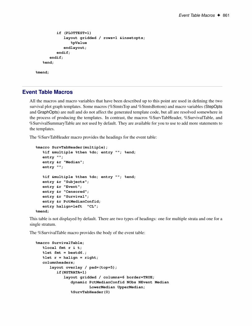
Event Table MacrosAll the macros and macro variables that have been described up to this point are used in defining the twosurvival plot graph templates. Some macros (%StmtsTop and %StmtsBottom) and macro variables (StepOptsand GraphOpts) are null and do not affect the generated template code, but all are resolved somewhere inthe process of producing the templates. In contrast, the macros %SurvTabHeader, %SurvivalTable, and%SurvivalSummaryTable are not used by default. They are available for you to use to add more statements tothe templates.
The %SurvTabHeader macro provides the headings for the event table:
%macro SurvTabHeader(multiple);%if &multiple %then %do; entry ""; %end;entry "";entry &r "Median";entry "";
%if &multiple %then %do; entry ""; %end;entry &r "Subjects";entry &r "Event";entry &r "Censored";entry &r "Survival";entry &r PctMedianConfid;entry halign=left "CL";
%mend;
This table is not displayed by default. There are two types of headings: one for multiple strata and one for asingle stratum.
The %SurvivalTable macro provides the body of the event table:
%macro SurvivalTable;%local fmt r i t;%let fmt = bestd6.;%let r = halign = right;columnheaders;
layout overlay / pad=(top=5);if(NSTRATA=1)
layout gridded / columns=6 border=TRUE;dynamic PctMedianConfid NObs NEvent Median
LowerMedian UpperMedian;%SurvTabHeader(0)
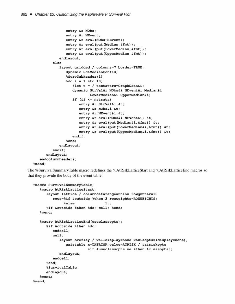
862 F Chapter 23: Customizing the Kaplan-Meier Survival Plot
entry &r NObs;entry &r NEvent;entry &r eval(NObs-NEvent);entry &r eval(put(Median,&fmt));entry &r eval(put(LowerMedian,&fmt));entry &r eval(put(UpperMedian,&fmt));
endlayout;else
layout gridded / columns=7 border=TRUE;dynamic PctMedianConfid;%SurvTabHeader(1)%do i = 1 %to 10;
%let t = / textattrs=GraphData&i;dynamic StrVal&i NObs&i NEvent&i Median&i
LowerMedian&i UpperMedian&i;if (&i <= nstrata)
entry &r StrVal&i &t;entry &r NObs&i &t;entry &r NEvent&i &t;entry &r eval(NObs&i-NEvent&i) &t;entry &r eval(put(Median&i,&fmt)) &t;entry &r eval(put(LowerMedian&i,&fmt)) &t;entry &r eval(put(UpperMedian&i,&fmt)) &t;
endif;%end;
endlayout;endif;
endlayout;endcolumnheaders;
%mend;
The %SurvivalSummaryTable macro redefines the %AtRiskLatticeStart and %AtRiskLatticeEnd macros sothat they provide the body of the event table:
%macro SurvivalSummaryTable;%macro AtRiskLatticeStart;
layout lattice / columndatarange=union rowgutter=10rows=%if &outside %then 2 rowweights=ROWWEIGHTS;
%else 1;;%if &outside %then %do; cell; %end;
%mend;
%macro AtRiskLatticeEnd(useclassopts);%if &outside %then %do;
endcell;cell;
layout overlay / walldisplay=none xaxisopts=(display=none);axistable x=TATRISK value=ATRISK / &atriskopts
%if &useclassopts ne %then &classopts;;endlayout;
endcell;%end;%SurvivalTableendlayout;
%mend;%mend;

Dynamic Variables F 863
If you want to create an event table like the one displayed in Figure 23.30, you only need to call the %Sur-vivalSummaryTable macro. If you want to modify the table, then you need to modify the %SurvTabHeaderand %SurvivalTable macros.
Dynamic VariablesGraph templates consist of instructions, written by SAS developers, in conjunction with SAS procedurecode. However, SAS developers cannot fully provide some instructions when the template is written, becausesome elements of some graphs cannot be known until the procedure runs. For example, the legend title in agraph that has multiple strata corresponds to the label or name of the stratification variable, and the procedurecalculates the p-value for the homogeneity test. SAS procedures create dynamic variables to provide somerun-time information to graphs.8 Some dynamic variables are set by the procedure and are declared in thetemplate. Other dynamic variables are also set by the procedure, but you must declare them directly orthrough the template modification macros before you can use them.
Dynamic Variables That Are Automatically DeclaredThe primary dynamic variables are as follows:
_ByFootNote_ is a binary variable that, when true, displays the BY-group BY line as a footnote.
_ByLine_ is a character variable that provides the BY-group BY line.
_ByTitle_ is a binary variable that, when true, displays the BY-group BY line as a title.
ClassAtRisk is a character variable that names the data object column that contains the classification(stratification) values.
GroupName is a character variable that contains the stratification legend title.
LabelCL is a character variable that contains the label for the confidence limits legend entry(including the percent sign).
LabelEP is a character variable that contains the label for the equal-precision band legend entry(including the percent sign).
LabelHW is a character variable that contains the label for the Hall-Wellner band legend entry(including the percent sign).
MaxTime is a numeric variable that contains the maximum value to display on the X axis.
Method is a character variable that contains the method for the plot title.
NStrata is an integer variable that contains the number of strata.
PValue is a numeric variable that contains the p-value for the homogeneity test.
PlotAtRisk is a binary variable that, when true, is used to display the at-risk table.
PlotCensored is a binary variable that, when true, displays the censored values on the step functions.
8Axis labels can be set directly in the template or at run time through dynamic variables or through data object column labels.
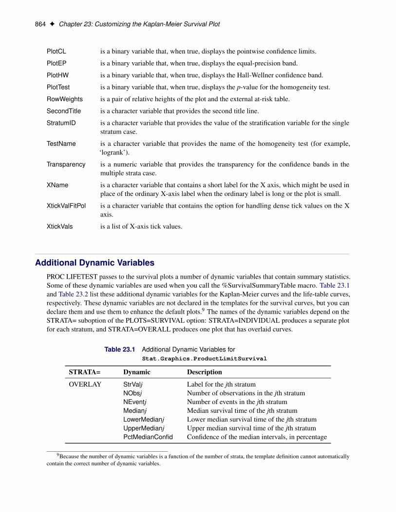
864 F Chapter 23: Customizing the Kaplan-Meier Survival Plot
PlotCL is a binary variable that, when true, displays the pointwise confidence limits.
PlotEP is a binary variable that, when true, displays the equal-precision band.
PlotHW is a binary variable that, when true, displays the Hall-Wellner confidence band.
PlotTest is a binary variable that, when true, displays the p-value for the homogeneity test.
RowWeights is a pair of relative heights of the plot and the external at-risk table.
SecondTitle is a character variable that provides the second title line.
StratumID is a character variable that provides the value of the stratification variable for the singlestratum case.
TestName is a character variable that provides the name of the homogeneity test (for example,‘logrank’).
Transparency is a numeric variable that provides the transparency for the confidence bands in themultiple strata case.
XName is a character variable that contains a short label for the X axis, which might be used inplace of the ordinary X-axis label when the ordinary label is long or the plot is small.
XtickValFitPol is a character variable that contains the option for handling dense tick values on the Xaxis.
XtickVals is a list of X-axis tick values.
Additional Dynamic VariablesPROC LIFETEST passes to the survival plots a number of dynamic variables that contain summary statistics.Some of these dynamic variables are used when you call the %SurvivalSummaryTable macro. Table 23.1and Table 23.2 list these additional dynamic variables for the Kaplan-Meier curves and the life-table curves,respectively. These dynamic variables are not declared in the templates for the survival curves, but you candeclare them and use them to enhance the default plots.9 The names of the dynamic variables depend on theSTRATA= suboption of the PLOTS=SURVIVAL option: STRATA=INDIVIDUAL produces a separate plotfor each stratum, and STRATA=OVERALL produces one plot that has overlaid curves.
Table 23.1 Additional Dynamic Variables forStat.Graphics.ProductLimitSurvival
STRATA= Dynamic Description
OVERLAY StrValj Label for the jth stratumNObsj Number of observations in the jth stratumNEventj Number of events in the jth stratumMedianj Median survival time of the jth stratumLowerMedianj Lower median survival time of the jth stratumUpperMedianj Upper median survival time of the jth stratumPctMedianConfid Confidence of the median intervals, in percentage
9Because the number of dynamic variables is a function of the number of strata, the template definition cannot automaticallycontain the correct number of dynamic variables.
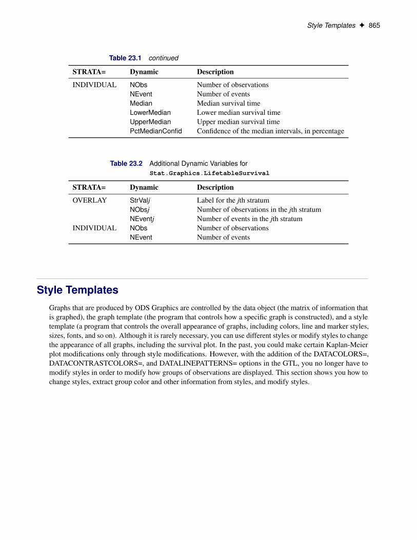
Style Templates F 865
Table 23.1 continued
STRATA= Dynamic Description
INDIVIDUAL NObs Number of observationsNEvent Number of eventsMedian Median survival timeLowerMedian Lower median survival timeUpperMedian Upper median survival timePctMedianConfid Confidence of the median intervals, in percentage
Table 23.2 Additional Dynamic Variables forStat.Graphics.LifetableSurvival
STRATA= Dynamic Description
OVERLAY StrValj Label for the jth stratumNObsj Number of observations in the jth stratumNEventj Number of events in the jth stratum
INDIVIDUAL NObs Number of observationsNEvent Number of events
Style TemplatesGraphs that are produced by ODS Graphics are controlled by the data object (the matrix of information thatis graphed), the graph template (the program that controls how a specific graph is constructed), and a styletemplate (a program that controls the overall appearance of graphs, including colors, line and marker styles,sizes, fonts, and so on). Although it is rarely necessary, you can use different styles or modify styles to changethe appearance of all graphs, including the survival plot. In the past, you could make certain Kaplan-Meierplot modifications only through style modifications. However, with the addition of the DATACOLORS=,DATACONTRASTCOLORS=, and DATALINEPATTERNS= options in the GTL, you no longer have tomodify styles in order to modify how groups of observations are displayed. This section shows you how tochange styles, extract group color and other information from styles, and modify styles.
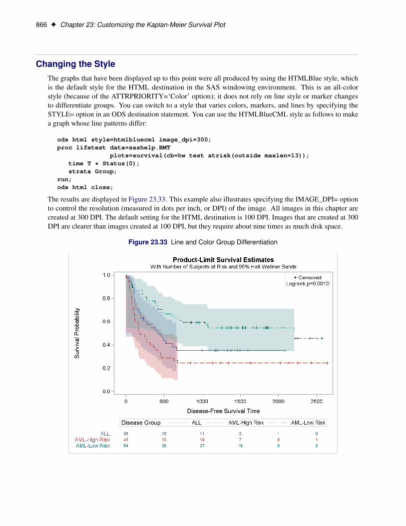
866 F Chapter 23: Customizing the Kaplan-Meier Survival Plot
Changing the StyleThe graphs that have been displayed up to this point were all produced by using the HTMLBlue style, whichis the default style for the HTML destination in the SAS windowing environment. This is an all-colorstyle (because of the ATTRPRIORITY=‘Color’ option); it does not rely on line style or marker changesto differentiate groups. You can switch to a style that varies colors, markers, and lines by specifying theSTYLE= option in an ODS destination statement. You can use the HTMLBlueCML style as follows to makea graph whose line patterns differ:
ods html style=htmlbluecml image_dpi=300;proc lifetest data=sashelp.BMT
plots=survival(cb=hw test atrisk(outside maxlen=13));time T * Status(0);strata Group;
run;ods html close;
The results are displayed in Figure 23.33. This example also illustrates specifying the IMAGE_DPI= optionto control the resolution (measured in dots per inch, or DPI) of the image. All images in this chapter arecreated at 300 DPI. The default setting for the HTML destination is 100 DPI. Images that are created at 300DPI are clearer than images created at 100 DPI, but they require about nine times as much disk space.
Figure 23.33 Line and Color Group Differentiation
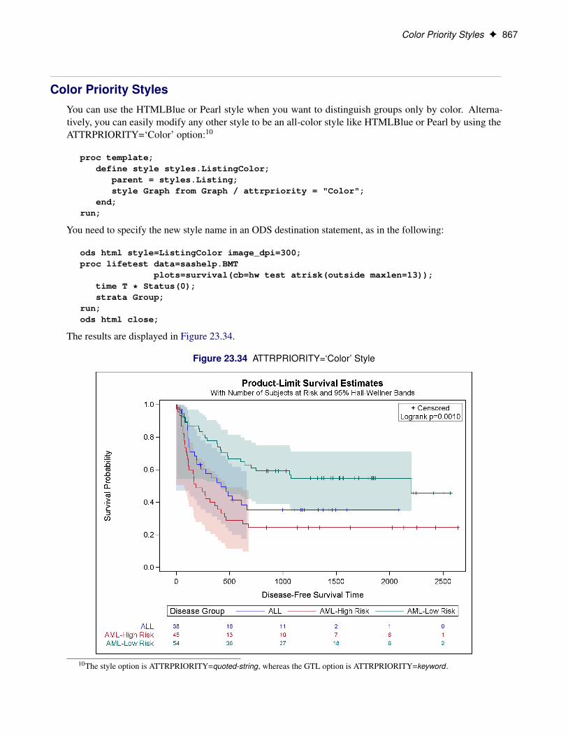
Color Priority Styles F 867
Color Priority StylesYou can use the HTMLBlue or Pearl style when you want to distinguish groups only by color. Alterna-tively, you can easily modify any other style to be an all-color style like HTMLBlue or Pearl by using theATTRPRIORITY=‘Color’ option:10
proc template;define style styles.ListingColor;
parent = styles.Listing;style Graph from Graph / attrpriority = "Color";
end;run;
You need to specify the new style name in an ODS destination statement, as in the following:
ods html style=ListingColor image_dpi=300;proc lifetest data=sashelp.BMT
plots=survival(cb=hw test atrisk(outside maxlen=13));time T * Status(0);strata Group;
run;ods html close;
The results are displayed in Figure 23.34.
Figure 23.34 ATTRPRIORITY=‘Color’ Style
10The style option is ATTRPRIORITY=quoted-string, whereas the GTL option is ATTRPRIORITY=keyword .
868 F Chapter 23: Customizing the Kaplan-Meier Survival Plot
Displaying a Style and Extracting Color ListsYou can use PROC TEMPLATE with the SOURCE statement to display a style as follows:
proc template;source styles.htmlblue;
run;
The results of this step, which are not shown, include the option PARENT=STYLES.STATISTICAL and donot include definitions of the colors (gData1, gData2, ..., gData12) and contrast colors (gcData1, gcData2,..., gcData12). These are the color definitions that are used in the style elements GraphData1, GraphData2,..., GraphData12. You can examine the parent Statistical style as follows:
proc template;source styles.statistical;
run;
The results of this step are not shown because they are hard to interpret in their raw form, but the desiredcolor definitions are included. You can submit the following statements to display the colors for the Statistical(and hence HTMLBlue) style in a more understandable form:
proc template;source styles.statistical / file='style.tmp';
run;
data colors;length element Color $ 20;infile 'style.tmp';input;if index(_infile_, 'data') then do;
element = scan(_infile_, 1, ' ');Color = scan(_infile_, 3, ' ;');Type = ifc(index(element, 'gc'), 'Line', 'Fill') || ' Colors';i = input(compress(element, 'gcdat'';'), ?? 2.);if i then output;
end;run;
proc sort; by descending type i; run;
proc print; id type; by descending type; var color; run;
The results are displayed in Figure 23.35. All colors are specified in values of the form CXrrggbb, where thelast six characters specify RGB (red, green, blue) values on the hexadecimal scale of 00 to FF (0 to 255, base10).
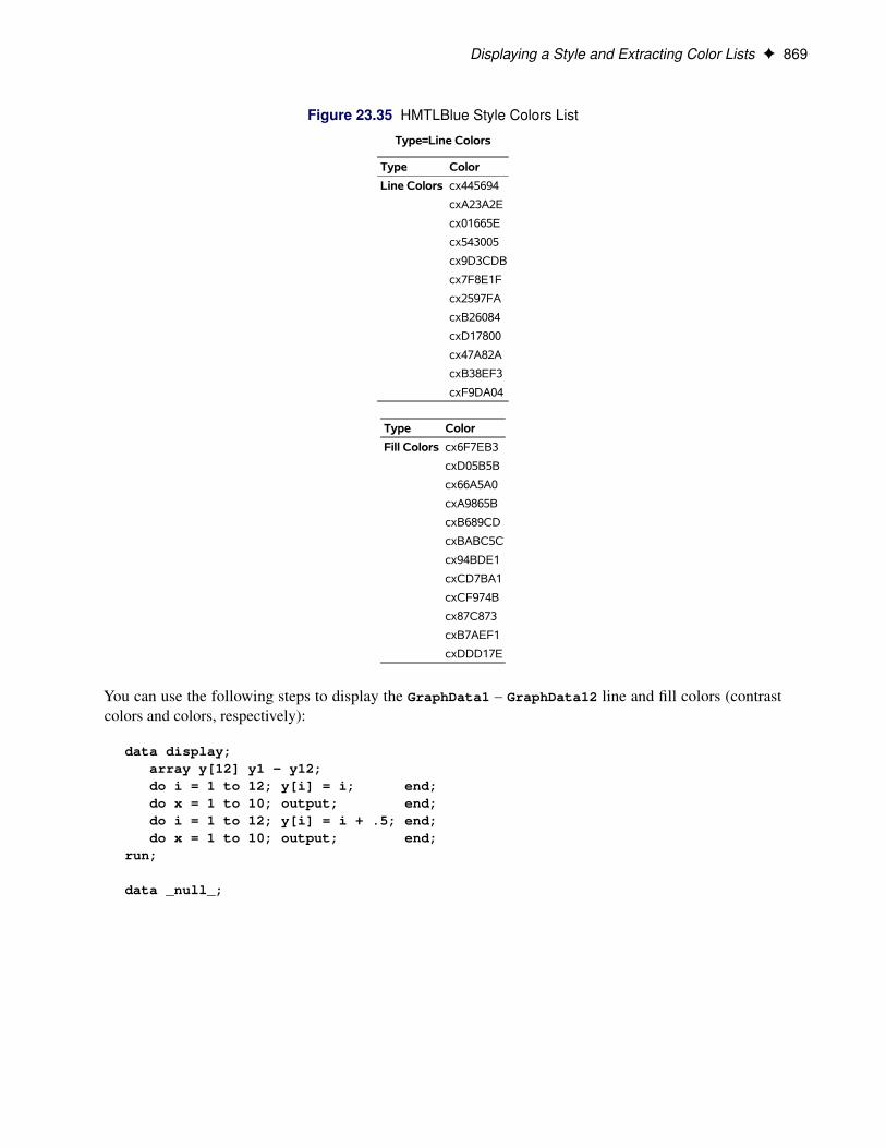
Displaying a Style and Extracting Color Lists F 869
Figure 23.35 HMTLBlue Style Colors List
Type=Line Colors
Type Color
Line Colors cx445694
cxA23A2E
cx01665E
cx543005
cx9D3CDB
cx7F8E1F
cx2597FA
cxB26084
cxD17800
cx47A82A
cxB38EF3
cxF9DA04
Type Color
Fill Colors cx6F7EB3
cxD05B5B
cx66A5A0
cxA9865B
cxB689CD
cxBABC5C
cx94BDE1
cxCD7BA1
cxCF974B
cx87C873
cxB7AEF1
cxDDD17E
You can use the following steps to display the GraphData1 – GraphData12 line and fill colors (contrastcolors and colors, respectively):
data display;array y[12] y1 - y12;do i = 1 to 12; y[i] = i; end;do x = 1 to 10; output; end;do i = 1 to 12; y[i] = i + .5; end;do x = 1 to 10; output; end;
run;
data _null_;
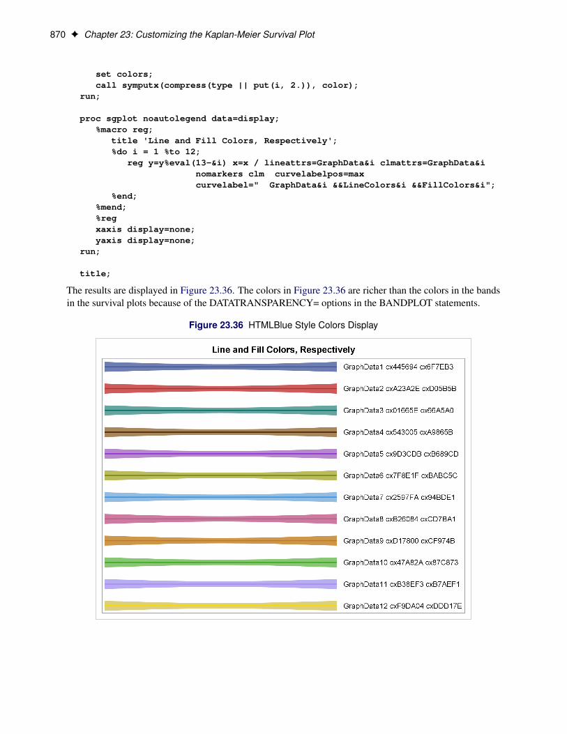
870 F Chapter 23: Customizing the Kaplan-Meier Survival Plot
set colors;call symputx(compress(type || put(i, 2.)), color);
run;
proc sgplot noautolegend data=display;%macro reg;
title 'Line and Fill Colors, Respectively';%do i = 1 %to 12;
reg y=y%eval(13-&i) x=x / lineattrs=GraphData&i clmattrs=GraphData&inomarkers clm curvelabelpos=maxcurvelabel=" GraphData&i &&LineColors&i &&FillColors&i";
%end;%mend;%regxaxis display=none;yaxis display=none;
run;
title;
The results are displayed in Figure 23.36. The colors in Figure 23.36 are richer than the colors in the bandsin the survival plots because of the DATATRANSPARENCY= options in the BANDPLOT statements.
Figure 23.36 HTMLBlue Style Colors Display
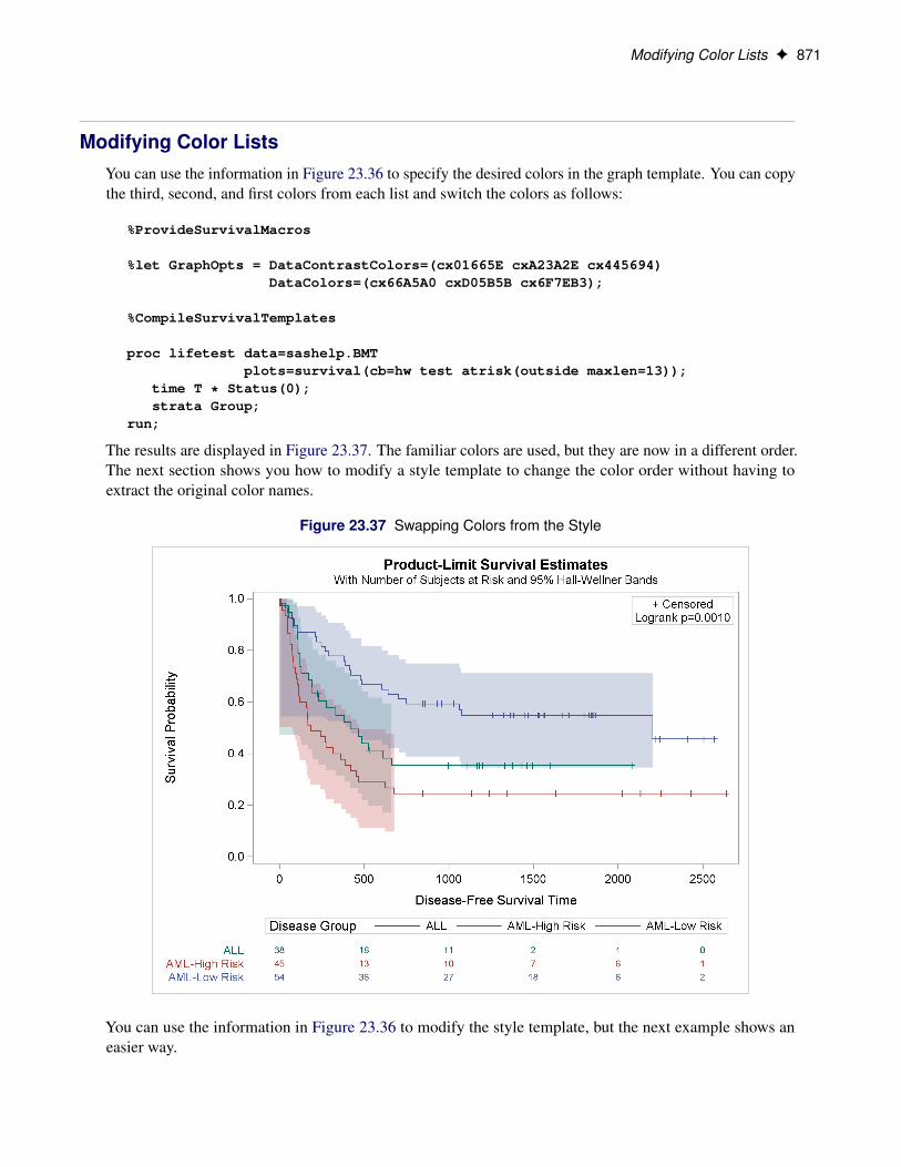
Modifying Color Lists F 871
Modifying Color ListsYou can use the information in Figure 23.36 to specify the desired colors in the graph template. You can copythe third, second, and first colors from each list and switch the colors as follows:
%ProvideSurvivalMacros
%let GraphOpts = DataContrastColors=(cx01665E cxA23A2E cx445694)DataColors=(cx66A5A0 cxD05B5B cx6F7EB3);
%CompileSurvivalTemplates
proc lifetest data=sashelp.BMTplots=survival(cb=hw test atrisk(outside maxlen=13));
time T * Status(0);strata Group;
run;
The results are displayed in Figure 23.37. The familiar colors are used, but they are now in a different order.The next section shows you how to modify a style template to change the color order without having toextract the original color names.
Figure 23.37 Swapping Colors from the Style
You can use the information in Figure 23.36 to modify the style template, but the next example shows aneasier way.

872 F Chapter 23: Customizing the Kaplan-Meier Survival Plot
Swapping Colors among Style ElementsYou can modify the colors in a style as follows:
%macro reorder(from, to, list);
proc template;define style styles.&to;
parent=styles.&from;%do i = 1 %to 12;
%let s = %scan(&list, &i);%if &s ne %then %do;
style GraphData&i from GraphData&i /contrastcolor = GraphColors("gcdata&s")color = GraphColors("gdata&s");
%end;%end;
end;run;
%mend;
%reorder(htmlblue, /* Parent style. */MyStyle, /* New style to create. Specify it in an ODS */
/* destination statement. */3 2 1) /* Replace the first few GraphData colors */
/* (1 2 3) with the colors from the specified *//* GraphData style elements (3 2 1). *//* You can specify up to 12 integers in the *//* range 1 - 12. */
The %Reorder macro creates a new style called MyStyle that inherits most of its attributes from theHTMLBlue style. However, in the new style, the colors for groups 1, 2, and 3 have been replaced bythe colors for groups 3, 2, and 1. In other words, the colors for GraphData1 and GraphData3 have beenswitched.
The following step creates the plot:
ods html style=mystyle;proc lifetest data=sashelp.BMT
plots=survival(cb=hw test atrisk(outside maxlen=13));time T * Status(0);strata Group;
run;ods html close;
The survival plot is not shown, but it matches the plot in Figure 23.37.
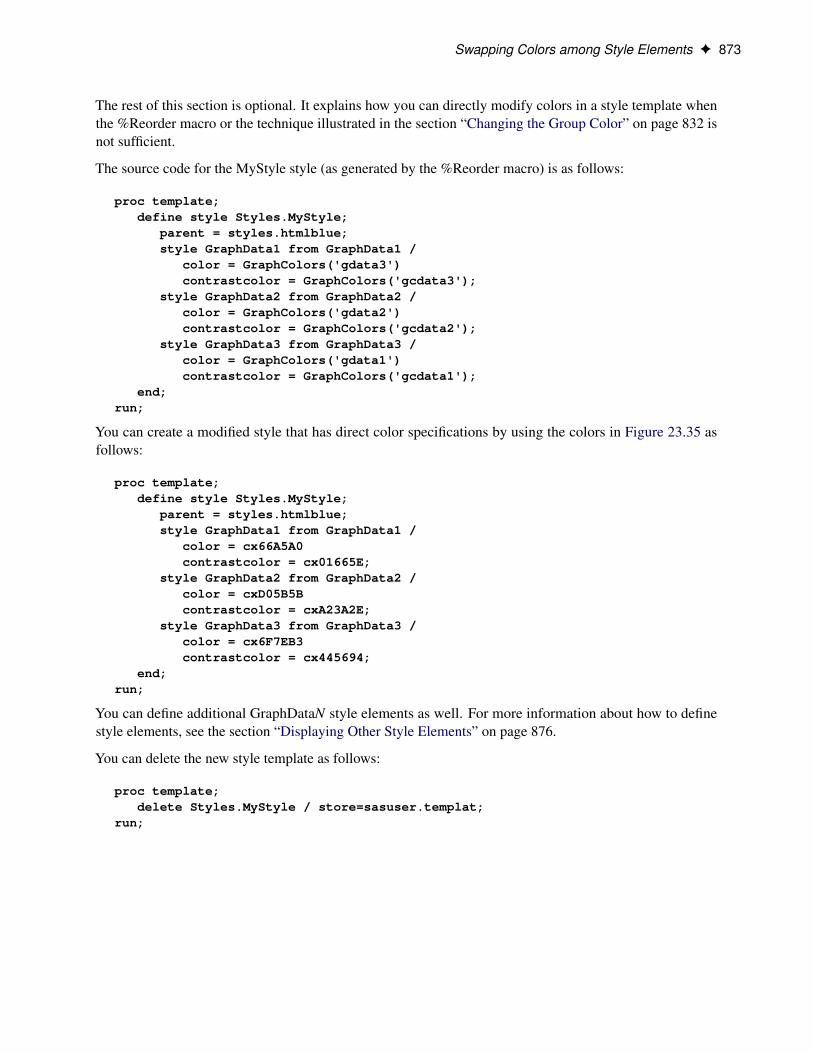
Swapping Colors among Style Elements F 873
The rest of this section is optional. It explains how you can directly modify colors in a style template whenthe %Reorder macro or the technique illustrated in the section “Changing the Group Color” on page 832 isnot sufficient.
The source code for the MyStyle style (as generated by the %Reorder macro) is as follows:
proc template;define style Styles.MyStyle;
parent = styles.htmlblue;style GraphData1 from GraphData1 /
color = GraphColors('gdata3')contrastcolor = GraphColors('gcdata3');
style GraphData2 from GraphData2 /color = GraphColors('gdata2')contrastcolor = GraphColors('gcdata2');
style GraphData3 from GraphData3 /color = GraphColors('gdata1')contrastcolor = GraphColors('gcdata1');
end;run;
You can create a modified style that has direct color specifications by using the colors in Figure 23.35 asfollows:
proc template;define style Styles.MyStyle;
parent = styles.htmlblue;style GraphData1 from GraphData1 /
color = cx66A5A0contrastcolor = cx01665E;
style GraphData2 from GraphData2 /color = cxD05B5Bcontrastcolor = cxA23A2E;
style GraphData3 from GraphData3 /color = cx6F7EB3contrastcolor = cx445694;
end;run;
You can define additional GraphDataN style elements as well. For more information about how to definestyle elements, see the section “Displaying Other Style Elements” on page 876.
You can delete the new style template as follows:
proc template;delete Styles.MyStyle / store=sasuser.templat;
run;
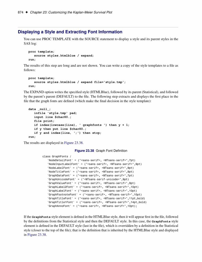
874 F Chapter 23: Customizing the Kaplan-Meier Survival Plot
Displaying a Style and Extracting Font InformationYou can use PROC TEMPLATE with the SOURCE statement to display a style and its parent styles in theSAS log:
proc template;source styles.htmlblue / expand;
run;
The results of this step are long and are not shown. You can write a copy of the style templates to a file asfollows:
proc template;source styles.htmlblue / expand file='style.tmp';
run;
The EXPAND option writes the specified style (HTMLBlue), followed by its parent (Statistical), and followedby the parent’s parent (DEFAULT) to the file. The following step extracts and displays the first place in thefile that the graph fonts are defined (which make the final decision in the style template):
data _null_;infile 'style.tmp' pad;input line $char80.;file print;if index(lowcase(line), ' graphfonts ') then y + 1;if y then put line $char80.;if y and index(line, ';') then stop;
run;
The results are displayed in Figure 23.38.
Figure 23.38 Graph Font Definition
class GraphFonts / 'NodeDetailFont' = ("<sans-serif>, <MTsans-serif>",7pt) 'NodeInputLabelFont' = ("<sans-serif>, <MTsans-serif>",9pt) 'NodeLabelFont' = ("<sans-serif>, <MTsans-serif>",9pt) 'NodeTitleFont' = ("<sans-serif>, <MTsans-serif>",9pt) 'GraphDataFont' = ("<sans-serif>, <MTsans-serif>",7pt) 'GraphUnicodeFont' = ("<MTsans-serif-unicode>",9pt) 'GraphValueFont' = ("<sans-serif>, <MTsans-serif>",9pt) 'GraphLabel2Font' = ("<sans-serif>, <MTsans-serif>",10pt) 'GraphLabelFont' = ("<sans-serif>, <MTsans-serif>",10pt) 'GraphFootnoteFont' = ("<sans-serif>, <MTsans-serif>",10pt) 'GraphTitleFont' = ("<sans-serif>, <MTsans-serif>",11pt,bold) 'GraphTitle1Font' = ("<sans-serif>, <MTsans-serif>",14pt,bold) 'GraphAnnoFont' = ("<sans-serif>, <MTsans-serif>",10pt);
If the GraphFonts style element is defined in the HTMLBlue style, then it will appear first in the file, followedby the definitions from the Statistical style and then the DEFAULT style. In this case, the GraphFonts styleelement is defined in the DEFAULT style (last in the file), which is overridden by a definition in the Statisticalstyle (closer to the top of the file); that is the definition that is inherited by the HTMLBlue style and displayedin Figure 23.38.
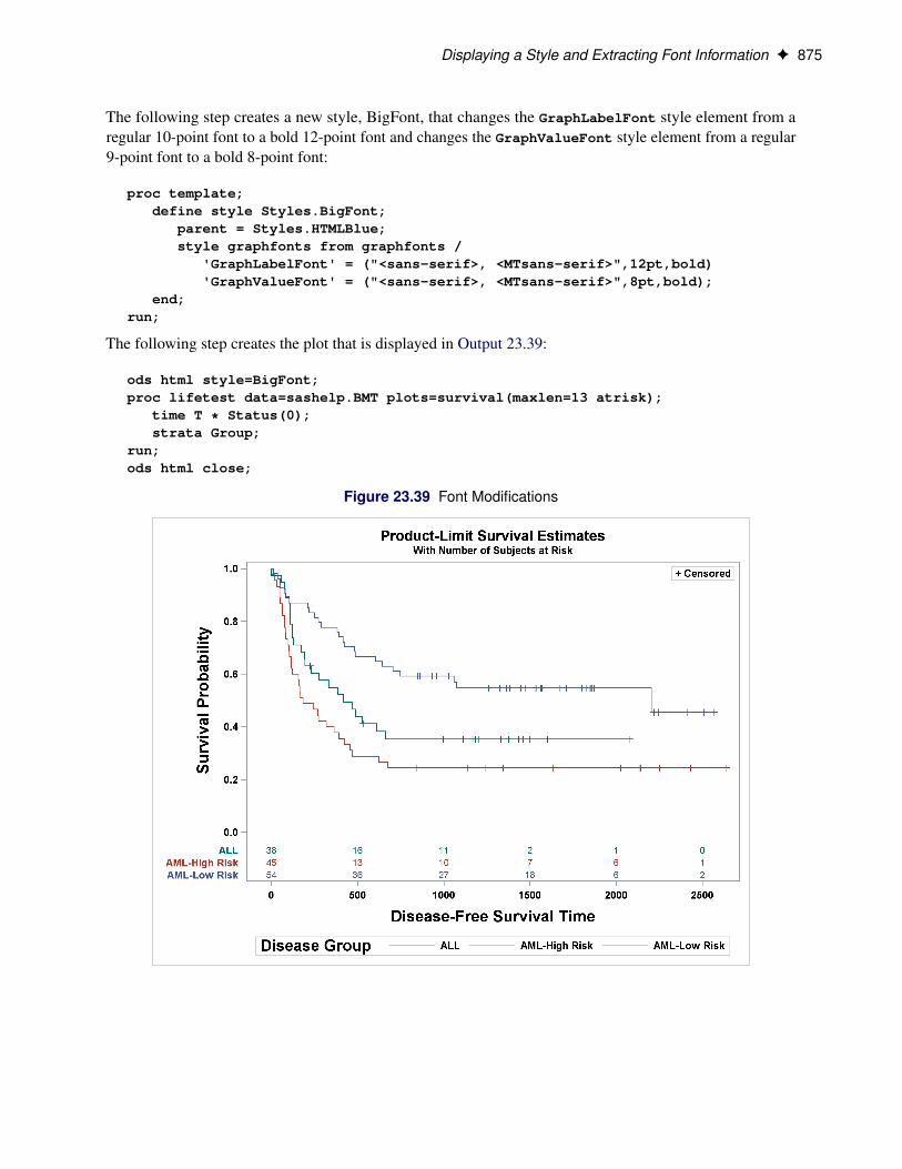
Displaying a Style and Extracting Font Information F 875
The following step creates a new style, BigFont, that changes the GraphLabelFont style element from aregular 10-point font to a bold 12-point font and changes the GraphValueFont style element from a regular9-point font to a bold 8-point font:
proc template;define style Styles.BigFont;
parent = Styles.HTMLBlue;style graphfonts from graphfonts /
'GraphLabelFont' = ("<sans-serif>, <MTsans-serif>",12pt,bold)'GraphValueFont' = ("<sans-serif>, <MTsans-serif>",8pt,bold);
end;run;
The following step creates the plot that is displayed in Output 23.39:
ods html style=BigFont;proc lifetest data=sashelp.BMT plots=survival(maxlen=13 atrisk);
time T * Status(0);strata Group;
run;ods html close;
Figure 23.39 Font Modifications
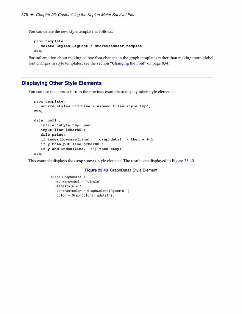
876 F Chapter 23: Customizing the Kaplan-Meier Survival Plot
You can delete the new style template as follows:
proc template;delete Styles.BigFont / store=sasuser.templat;
run;
For information about making ad hoc font changes in the graph templates rather than making more globalfont changes in style templates, see the section “Changing the Font” on page 834.
Displaying Other Style ElementsYou can use the approach from the previous example to display other style elements:
proc template;source styles.htmlblue / expand file='style.tmp';
run;
data _null_;infile 'style.tmp' pad;input line $char80.;file print;if index(lowcase(line), ' graphdata1 ') then y + 1;if y then put line $char80.;if y and index(line, ';') then stop;
run;
This example displays the GraphData1 style element. The results are displayed in Figure 23.40.
Figure 23.40 GraphData1 Style Element
class GraphData1 / markersymbol = "circle" linestyle = 1 contrastcolor = GraphColors('gcdata1') color = GraphColors('gdata1');
Displaying Other Style Elements F 877
The following steps display all the GraphFonts style elements from all the styles:
proc template;source styles / file='style.tmp';
run;
data _null_;infile 'style.tmp' pad;length style $ 80;retain style;input line $char80.;file print;if index(lowcase(line), 'define style') then style = line;if index(lowcase(line), ' graphfonts ') then do;
y + 1;put style $char80.;
end;if y then put line $char80.;if index(line, ';') then y = 0;;
run;
The results of this step are not displayed. You can use this approach to help you better understand theoptions that are available for modifying styles. The SOURCE statement specifies a single-level value ofSTYLES rather than a specific style name such as STYLES.HTMLBLUE, so all templates that begin withSTYLES as the first level (all style templates) are written to the file. The DATA step displays all definitionsof GraphFonts and the names of all styles that define the GraphFonts style element.
You can insert the name of another style element (in lowercase with a leading and trailing blank) in thepreceding programs in place of ‘graphdata1’ or ‘graphfonts’. After you display a style element, you canmodify the definition and create a new style that uses the modified definition, as in the example in the section“Displaying a Style and Extracting Font Information” on page 874. Some of the style elements that you mightwant to display and modify are listed in Table 23.3.
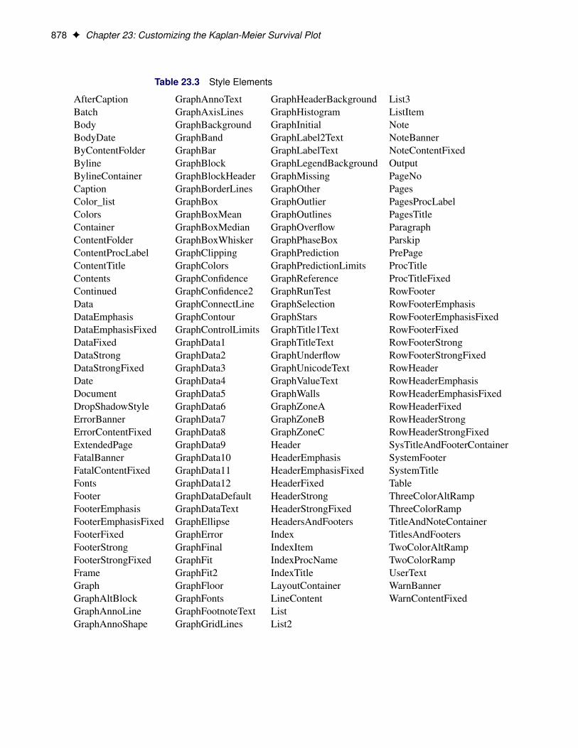
878 F Chapter 23: Customizing the Kaplan-Meier Survival Plot
Table 23.3 Style Elements
AfterCaption GraphAnnoText GraphHeaderBackground List3Batch GraphAxisLines GraphHistogram ListItemBody GraphBackground GraphInitial NoteBodyDate GraphBand GraphLabel2Text NoteBannerByContentFolder GraphBar GraphLabelText NoteContentFixedByline GraphBlock GraphLegendBackground OutputBylineContainer GraphBlockHeader GraphMissing PageNoCaption GraphBorderLines GraphOther PagesColor_list GraphBox GraphOutlier PagesProcLabelColors GraphBoxMean GraphOutlines PagesTitleContainer GraphBoxMedian GraphOverflow ParagraphContentFolder GraphBoxWhisker GraphPhaseBox ParskipContentProcLabel GraphClipping GraphPrediction PrePageContentTitle GraphColors GraphPredictionLimits ProcTitleContents GraphConfidence GraphReference ProcTitleFixedContinued GraphConfidence2 GraphRunTest RowFooterData GraphConnectLine GraphSelection RowFooterEmphasisDataEmphasis GraphContour GraphStars RowFooterEmphasisFixedDataEmphasisFixed GraphControlLimits GraphTitle1Text RowFooterFixedDataFixed GraphData1 GraphTitleText RowFooterStrongDataStrong GraphData2 GraphUnderflow RowFooterStrongFixedDataStrongFixed GraphData3 GraphUnicodeText RowHeaderDate GraphData4 GraphValueText RowHeaderEmphasisDocument GraphData5 GraphWalls RowHeaderEmphasisFixedDropShadowStyle GraphData6 GraphZoneA RowHeaderFixedErrorBanner GraphData7 GraphZoneB RowHeaderStrongErrorContentFixed GraphData8 GraphZoneC RowHeaderStrongFixedExtendedPage GraphData9 Header SysTitleAndFooterContainerFatalBanner GraphData10 HeaderEmphasis SystemFooterFatalContentFixed GraphData11 HeaderEmphasisFixed SystemTitleFonts GraphData12 HeaderFixed TableFooter GraphDataDefault HeaderStrong ThreeColorAltRampFooterEmphasis GraphDataText HeaderStrongFixed ThreeColorRampFooterEmphasisFixed GraphEllipse HeadersAndFooters TitleAndNoteContainerFooterFixed GraphError Index TitlesAndFootersFooterStrong GraphFinal IndexItem TwoColorAltRampFooterStrongFixed GraphFit IndexProcName TwoColorRampFrame GraphFit2 IndexTitle UserTextGraph GraphFloor LayoutContainer WarnBannerGraphAltBlock GraphFonts LineContent WarnContentFixedGraphAnnoLine GraphFootnoteText ListGraphAnnoShape GraphGridLines List2
SAS Item Stores F 879
SAS Item StoresIn other sections of this chapter, you submit PROC TEMPLATE statements (either directly or throughmacros) to compile and save graph and style templates. Compiled templates are stored in special SAS filescalled item stores. Assuming that you have not modified your ODS path with an ODS PATH statement, thetemplates that you compile are stored in an item store in the Sasuser library. By default, all templates thatSAS provides are stored in an item store in the Sashelp library. By default, the Sashelp item store has readaccess only; you cannot write to it. By default, the Sasuser item store has update access; you can both readand write to it. CAUTION: Never set the Sashelp item store to update or write access. If you do, and if youhave administrator privileges on your computer, you could corrupt the Sashelp item store.
Assuming that the default ODS path is used, ODS first looks for a template in the Sasuser item store. Ifit does not find the template there, ODS next looks for the template in the Sashelp item store. Files in theSasuser library persist across SAS sessions until you delete them. You can run the following step to deletethe entire Sasuser item store (including all compiled graph and style templates that you added or modified)so that ODS uses only the templates the SAS System supplies:
ods path sashelp.tmplmst(read);proc datasets library=sasuser nolist;
delete templat(memtype=itemstor);run;ods path reset;
For more information about the ODS path and SAS item stores, see Chapter 21, “Statistical Graphics UsingODS.”
References
Hall, W. J., and Wellner, J. A. (1980). “Confidence Bands for a Survival Curve from Censored Data.”Biometrika 67:133–143.
Kaplan, E. L., and Meier, P. (1958). “Nonparametric Estimation from Incomplete Observations.” Journal ofthe American Statistical Association 53:457–481.
Klein, J. P., and Moeschberger, M. L. (1997). Survival Analysis: Techniques for Censored and TruncatedData. New York: Springer-Verlag.
Index
p valueLIFETEST procedure, 841
ACROSS= GTL optionLIFETEST procedure, 836
at-risk table (inside)LIFETEST procedure, 814
at-risk table (outside)LIFETEST procedure, 816
at-risk value specificationLIFETEST procedure, 817–819
ATRISK survival-plot optionLIFETEST procedure, 814
ATRISK(MAXLEN=13) survival-plot optionLIFETEST procedure, 815
ATRISK(OUTSIDE) survival-plot optionLIFETEST procedure, 816
ATRISK= survival-plot optionLIFETEST procedure, 817
%AtRiskLatticeEnd macroLIFETEST procedure, 858
%AtRiskLatticeStart macroLIFETEST procedure, 858
ATRISKTICK survival-plot optionLIFETEST procedure, 818
ATRISKTICKONLY survival-plot optionLIFETEST procedure, 819
ATTRPRIORITY=’Color’ styleLIFETEST procedure, 867
ATTRPRIORITY=NONE GTL optionLIFETEST procedure, 833
AUTOALIGN= GTL optionLIFETEST procedure, 836, 844
axis label modificationLIFETEST procedure, 829
CB=ALL survival-plot optionLIFETEST procedure, 812
CB=EP survival-plot optionLIFETEST procedure, 812
CB=HW survival-plot optionLIFETEST procedure, 811
Censored macro variableLIFETEST procedure, 838
censored value legendLIFETEST procedure, 823
CensorStr macro variableLIFETEST procedure, 838
%CompileSurvivalTemplates macro
LIFETEST procedure, 827, 857
DATACOLORS= GTL optionLIFETEST procedure, 832, 871
DATACONTRASTCOLORS= GTL optionLIFETEST procedure, 832, 871
DATALINEPATTERNS= GTL optionLIFETEST procedure, 833
date (displaying in a footnote)LIFETEST procedure, 843
DESIGNHEIGHT= GTL optionLIFETEST procedure, 849
DESIGNHEIGHT=500PX GTL optionLIFETEST procedure, 848
DESIGNHEIGHT=DEFAULTDESIGNWIDTH GTLoption
LIFETEST procedure, 846
ENTRYFOOTNOTE GTL statementLIFETEST procedure, 843
equal-precision bandsLIFETEST procedure, 812
event summary tableLIFETEST procedure, 846, 848
events (number of inset table)LIFETEST procedure, 844
EXPAND optionTEMPLATE procedure, 874
FAILURE survival-plot optionLIFETEST procedure, 824
FAMILY=GRAPHUNICODETEXT GTL optionLIFETEST procedure, 838
font changesLIFETEST procedure, 834
fontsLIFETEST procedure, 874–876
footnoteLIFETEST procedure, 843
formatLIFETEST procedure, 820, 822, 849
GraphDataN style element modificationLIFETEST procedure, 873
GraphOpts macro variableLIFETEST procedure, 832, 833, 846, 848, 849,
871group reordering
LIFETEST procedure, 820, 822
Hall-Wellner confidence bandsLIFETEST procedure, 811, 812
HTMLBlueCML styleLIFETEST procedure, 866
informatLIFETEST procedure, 820, 822, 849
insetLIFETEST procedure, 836
inset tableLIFETEST procedure, 844
InsetOpts macro variableLIFETEST procedure, 836, 844, 849
Kaplan-Meier plotLIFETEST procedure, 806, 807, 827
label modificationLIFETEST procedure, 829
legendLIFETEST procedure, 836
legend suppressionLIFETEST procedure, 848
LegendOpts macro variableLIFETEST procedure, 836, 844, 848
LIFETEST procedurep value, 841_ByFootNote_ dynamic variable, 863_ByLine_ dynamic variable, 863_ByTitle_ dynamic variable, 863ACROSS= GTL option, 836at-risk table (inside), 814at-risk table (outside), 816at-risk value specification, 817–819ATRISK survival-plot option, 814ATRISK(MAXLEN=13) survival-plot option, 815ATRISK(OUTSIDE) survival-plot option, 816ATRISK= survival-plot option, 817%AtRiskLatticeEnd macro, 858%AtRiskLatticeStart macro, 858AtRiskOpts macro variable defined, 855ATRISKTICK survival-plot option, 818ATRISKTICKONLY survival-plot option, 819ATTRPRIORITY= GTL option, 855ATTRPRIORITY=’Color’ style, 867ATTRPRIORITY=NONE GTL option, 833AUTOALIGN= GTL option, 836, 844axis label modification, 829BandOpts macro variable defined, 855CB=ALL survival-plot option, 812CB=EP survival-plot option, 812CB=HW survival-plot option, 811Censored macro variable, 838Censored macro variable defined, 855censored value legend, 823
CensorStr macro variable, 838CensorStr macro variable defined, 855ClassAtRisk dynamic variable, 863ClassOpts macro variable defined, 855%CompileSurvivalTemplates macro, 827, 857DATACOLORS= GTL option, 832, 855, 871DATACONTRASTCOLORS= GTL option, 832,
855, 871DATALINEPATTERNS= GTL option, 833, 855date (displaying in a footnote), 843DESIGNHEIGHT= GTL option, 849, 856DESIGNHEIGHT=500PX GTL option, 848DESIGNHEIGHT=DEFAULTDESIGNWIDTH
GTL option, 846DESIGNWIDTH= GTL option, 856ENTRYFOOTNOTE GTL statement, 843equal-precision bands, 812event summary table, 846, 848events (number of inset table), 844FAILURE survival-plot option, 824FAMILY=GRAPHUNICODETEXT GTL option,
838font changes, 834fonts, 874–876footnote, 843format, 820, 822, 849GraphDataN style element modification, 873GraphOpts macro variable, 832, 833, 846, 848,
849, 871GraphOpts macro variable defined, 855group reordering, 820, 822GroupName dynamic variable, 863Groups macro variable defined, 855Hall-Wellner confidence bands, 811, 812HTMLBlueCML style, 866informat, 820, 822, 849inset, 836inset table, 844InsetOpts macro variable, 836, 844, 849InsetOpts macro variable defined, 855Kaplan-Meier plot, 806, 807, 827label modification, 829LabelCL dynamic variable, 863LabelEP dynamic variable, 863LabelHW dynamic variable, 863legend, 836legend suppression, 848LegendOpts macro variable, 836, 844, 848LegendOpts macro variable defined, 855line patterns, 833LINEATTRS=(THICKNESS=2.5) GTL option,
831LOCATION=INSIDE GTL option, 836, 844Log rank p value, 841
LowerMedian dynamic variable, 864macro variables, 853–856macros, 825MARKERATTRS= GTL option, 838MAXLEN=13 survival-plot option, 815MaxTime dynamic variable, 863Median dynamic variable, 864Method dynamic variable, 863%MultipleStrata macro, 860NAME= GTL option, 848, 849NEvent dynamic variable, 864NObs dynamic variable, 864NOCENSOR survival-plot option, 823NStrata dynamic variable, 863nTitles macro variable, 843, 849nTitles macro variable defined, 854ORDER= option, 820, 822OUTSIDE survival-plot option, 816patients-at-risk table (inside), 814patients-at-risk table (outside), 816PctMedianConfid dynamic variable, 864PlotAtRisk dynamic variable, 863PlotCensored dynamic variable, 863PlotCL dynamic variable, 864PlotEP dynamic variable, 864PlotHW dynamic variable, 864PLOTS=SURVIVAL, 808PlotTest dynamic variable, 864product-limit survival plot, 807%ProvideSurvivalMacros macro, 827PValue dynamic variable, 863%pValue macro, 856reference line, 839REFERENCELINE GTL statement, 839%Reorder macro, 872reordering groups, 820, 822RowWeights dynamic variable, 864sample library, 825SecondTitle dynamic variable, 864%SingleStratum macro, 859StepOpts macro variable, 831, 849StepOpts macro variable defined, 854%StmtsBeginGraph macro, 843, 856%StmtsBottom macro, 856%StmtsTop macro, 856STRATA=INDIVIDUAL survival-plot option,
809STRATA=PANEL survival-plot option, 809StratumID dynamic variable, 864StrVal dynamic variable, 864style change, 866, 872style cleanup, 873style color list modification, 871, 872style colors, 868, 869
summary of events table, 846, 848survival plot, 807%SurvivalSummaryTable macro, 862%SurvivalTable macro, 861%SurvTabHeader macro, 861template cleanup, 826, 842, 850, 879TEST survival-plot option, 811TestName dynamic variable, 864TEXTATTRS= GTL option, 834, 838tick value modification, 829TICKVALUELIST= GTL option, 829TipLabel macro variable defined, 854Tips macro variable defined, 854title change, 827TitleText0 macro variable, 834TitleText0 macro variable defined, 854TitleText1 macro variable, 834TitleText1 macro variable defined, 854TitleText2 macro variable, 834, 844, 849TitleText2 macro variable defined, 854Transparency dynamic variable, 864Unicode, 838UpperMedian dynamic variable, 864VIEWMIN= GTL option, 830XName dynamic variable, 864xOptions macro variable, 834xOptions macro variable defined, 854XtickValFitPol dynamic variable, 864XtickVals dynamic variable, 864yOptions macro variable, 829, 830, 834yOptions macro variable defined, 854
line patternsLIFETEST procedure, 833
LINEATTRS=(THICKNESS=2.5) GTL optionLIFETEST procedure, 831
LOCATION=INSIDE GTL optionLIFETEST procedure, 836, 844
Log rank p valueLIFETEST procedure, 841
macro variablesLIFETEST procedure, 853–856
macrosLIFETEST procedure, 825
MARKERATTRS= GTL optionLIFETEST procedure, 838
MAXLEN=13 survival-plot optionLIFETEST procedure, 815
%MultipleStrata macroLIFETEST procedure, 860
NAME= GTL optionLIFETEST procedure, 848, 849
NOCENSOR survival-plot option

LIFETEST procedure, 823nTitles macro variable
LIFETEST procedure, 843, 849
ORDER= optionLIFETEST procedure, 820, 822
OUTSIDE survival-plot optionLIFETEST procedure, 816
patients-at-risk table (inside)LIFETEST procedure, 814
patients-at-risk table (outside)LIFETEST procedure, 816
PLOTS=SURVIVALLIFETEST procedure, 808
product-limit survival plotLIFETEST procedure, 807
%ProvideSurvivalMacros macroLIFETEST procedure, 827
%pValue macroLIFETEST procedure, 856
reference lineLIFETEST procedure, 839
REFERENCELINE GTL statementLIFETEST procedure, 839
%Reorder macroLIFETEST procedure, 872
reordering groupsLIFETEST procedure, 820, 822
sample libraryLIFETEST procedure, 825
%SingleStratum macroLIFETEST procedure, 859
StepOpts macro variableLIFETEST procedure, 831, 849
%StmtsBeginGraph macroLIFETEST procedure, 843, 856
%StmtsBottom macroLIFETEST procedure, 856
%StmtsTop macroLIFETEST procedure, 856
STRATA=INDIVIDUAL survival-plot optionLIFETEST procedure, 809
STRATA=PANEL survival-plot optionLIFETEST procedure, 809
style changeLIFETEST procedure, 866, 872
style cleanupLIFETEST procedure, 873
style color list modificationLIFETEST procedure, 871, 872
style colorsLIFETEST procedure, 868, 869
summary of events tableLIFETEST procedure, 846, 848
survival plotLIFETEST procedure, 807
%SurvivalSummaryTable macroLIFETEST procedure, 862
%SurvivalTable macroLIFETEST procedure, 861
%SurvTabHeader macroLIFETEST procedure, 861
template cleanupLIFETEST procedure, 826, 842, 850, 879
TEMPLATE procedureEXPAND option, 874
TEST survival-plot optionLIFETEST procedure, 811
TEXTATTRS= GTL optionLIFETEST procedure, 834, 838
tick value modificationLIFETEST procedure, 829
TICKVALUELIST= GTL optionLIFETEST procedure, 829
title changeLIFETEST procedure, 827
TitleText0 macro variableLIFETEST procedure, 834
TitleText1 macro variableLIFETEST procedure, 834
TitleText2 macro variableLIFETEST procedure, 834, 844, 849
UnicodeLIFETEST procedure, 838
VIEWMIN= GTL optionLIFETEST procedure, 830
xOptions macro variableLIFETEST procedure, 834
yOptions macro variableLIFETEST procedure, 829, 830, 834
![A COMPARISON OF KAPLAN-MEIER AND CUMULATIVE INCIDENCE ...d-scholarship.pitt.edu/9986/1/BintuSherif_thesis[1].pdf · a comparison of kaplan-meier and cumulative incidence estimate](https://img.pdfslide.net/doc/110x75/5ad1fe937f8b9a92258c90e6/a-comparison-of-kaplan-meier-and-cumulative-incidence-d-1pdfa-comparison-of.jpg)