Embed Size (px)
Citation preview

Kaplan-Meier Survival
Curves and the Log-
Rank Test
Seminar in Statistics: Survival Analysis
Linda Staub & Alexandros Gekenidis
Chapter 2
March 7th, 2011

1 Review Outcome variable of interest: time until an event
occurs
Time = survival time
Event = failure
Censoring: Don‘t know survival time exactly
True survival time
observed survival time
Right-censored

1 Review 𝑇 = failure time with distribution 𝐹, density 𝑓
𝐶 = censoring time with distribution 𝐺, density 𝑔
Assume that the censoring time 𝐶 is
independent of the variable of interest 𝑇
𝑋 = min (𝑇, 𝐶), Δ = 1*𝑇≤𝐶+
We observe 𝑛 i.i.d. copies of (𝑋, Δ)
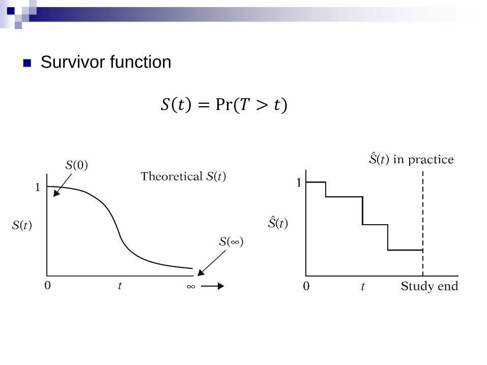
Survivor function
𝑆 𝑡 = Pr (𝑇 > 𝑡)

Alternative (Ordered) Data Layout
Risk set: collection of individuals who have survived at least to time 𝑡(𝑗)

2 Kaplan-Meier Curves
Example
The data: remission times (weeks) for two groups of
leukemia patients
6, 6, 6, 7, 10, 1, 1, 2, 2, 3,
13, 16, 22, 23, 4, 4, 5, 5,
6+, 9+, 10+, 11+, 8, 8, 8, 8,
17+, 19+, 20+, 11, 11, 12, 12,
25+, 32+, 32+, 15, 17, 22, 23
34+, 25+
+ denotes censored
Group 1 (n=21)
treatment
Group 2 (n=21)
placebo
Group 1 9 12 21
Group 2 21 0 21
# failed
# censored Total
Descriptive statistic:
6.8,1.17 21 TT 'signoring

Table of ordered failure times
0 21 0 0 0 21 0 0
6 21 3 1 1 21 2 0
7 17 1 1 2 19 2 0
10 15 1 2 3 17 1 0
13 12 1 0 4 16 2 0
16 11 1 3 5 14 2 0
22 7 1 0 8 12 4 0
23 6 1 5 11 8 2 0
>23 - - - 12 6 2 0
15 4 1 0
17 3 1 0
22 2 1 0
23 1 1 0
)( jt jn jm jq )( jt jn jm jq
Group 1 (treatment) Group 2 (placebo)
→ Remark: no censorship in group 2
6, 6, 6, 7, 10, 1, 1, 2, 2, 3,
13, 16, 22, 23, 4, 4, 5, 5,
6+, 9+, 10+, 11+, 8, 8, 8, 8,
17+, 19+, 20+, 11, 11, 12, 12,
25+, 32+, 32+, 15, 17, 22, 23
34+, 25+
+ denotes
censored
Group 1 (treatment) Group 2 (placebo)
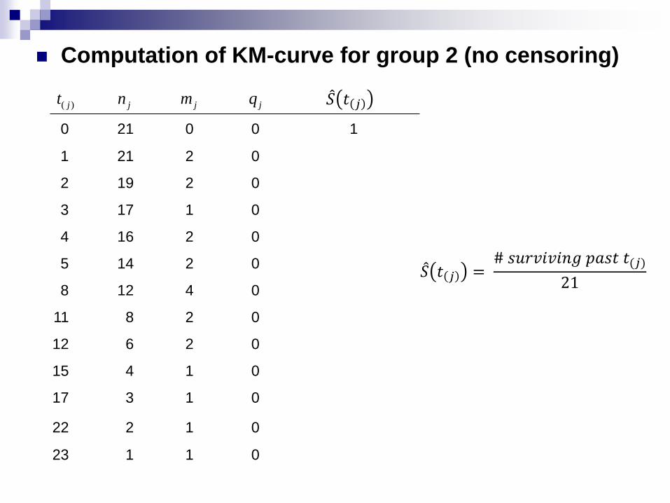
Computation of KM-curve for group 2 (no censoring)
0 21 0 0 1
1 21 2 0 19/21 = .90
2 19 2 0 17/21 = .81
3 17 1 0 16/21 = .76
4 16 2 0 14/21 = .67
5 14 2 0 12/21 = .57
8 12 4 0 8/21 = .38
11 8 2 0 6/21 = .29
12 6 2 0 4/21 = .19
15 4 1 0 3/21 = .14
17 3 1 0 2/21 = .10
22 2 1 0 1/21 = .05
23 1 1 0 0/21 = .00
)( jt jn jm jq
𝑆 𝑡 𝑗 = # 𝑠𝑢𝑟𝑣𝑖𝑣𝑖𝑛𝑔 𝑝𝑎𝑠𝑡 𝑡(𝑗)
21
𝑆 𝑡 𝑗

KM Curve for Group 2 (Placebo)
> time2 <-
c(1,1,2,2,3,4,4,5,5,8,8,8,8,11,11,12,12,15,17,
22,23)
> status2 <-
c(1,1,1,1,1,1,1,1,1,1,1,1,1,1,1,1,1,1,1,1,1)
> fit2 <- survfit(Surv(time2, status2) ~ 1)
> plot(fit2,conf.int=0, col = 'red', xlab =
'Time (weeks)', ylab = 'Survival Probability')
> title(main='KM Curve for Group 2 (placebo)')

General KM formula
Alternative way to calculate the survival probabilities
KM formula = product limit formula
𝑆 𝑡 𝑗 = 𝑃 𝑟 𝑇 > 𝑡(𝑖) 𝑇 ≥ 𝑡(𝑖)
𝑗
𝑖=1
= 𝑆 𝑡(𝑗−1) × 𝑃 𝑟 𝑇 > 𝑡(𝑗) 𝑇 ≥ 𝑡(𝑗)
Proof: blackboard

Computation of KM-curve for group 1
(treatment)
0 21 0 0 1
6 21 3 1 1×18/21=.8571
7 17 1 1 .8571×16/17=.8067
10 15 1 2 .8067×14/15=.7529
13 12 1 0 .7529×11/12=.6902
16 11 1 3 .6902×10/11=.6275
22 7 1 0 .6275×6/7=.5378
23 6 1 5 .5378×5/6=.4482
)( jt jn jm jq
Not available at
jt
jt
failed prior to
Censored prior to
jt
Fraction at 𝑡(𝑗):
Pr 𝑇 > 𝑡(𝑗) 𝑇 ≥ 𝑡(𝑗))
𝑆 𝑡(𝑗)
=𝑛𝑗 − 𝑚𝑗
𝑛𝑗

Computation of KM-curve for group 1
(treatment)
0 21 0 0 1
6 21 3 1 1×18/21=.8571
7 17 1 1 .8571×16/17=.8067
10 15 1 2 .8067×14/15=.7529
13 12 1 0 .7529×11/12=.6902
16 11 1 3 .6902×10/11=.6275
22 7 1 0 .6275×6/7=.5378
23 6 1 5 .5378×5/6=.4482
)( jt jn jm jq
Not available at
jt
jt
failed prior to
Censored prior to
jt
Fraction at 𝑡(𝑗):
Pr 𝑇 > 𝑡(𝑗) 𝑇 ≥ 𝑡(𝑗))
𝑆 𝑡(𝑗)

KM-curve for group 1 (treatment)
> time1 <-
c(6,6,6,7,10,13,16,22,23,6,9,10,11,17,19,20,
25,32,32,34,35)
> status1 <-
c(1,1,1,1,1,1,1,1,1,0,0,0,0,0,0,0,0,0,0,0,0)
> fit1 <- survfit(Surv(time1, status1) ~ 1)
> plot(fit1,conf.int=0, col = 'red', xlab =
'Time (weeks)', ylab = 'Survival
Probability')
> title(main='KM Curve for Group 1
(treatment)')

KM-estimator = Nonparametric MLE Model
𝑇 = failure time distr. function 𝐹, density 𝑓
𝐶 = censoring time distr. function 𝐺, density 𝑔
Assume that 𝐶 is independent of 𝑇
𝑋 = min (𝑇, 𝐶) Δ = 1*𝑇≤𝐶+
We observe 𝑛 i.i.d. copies of (𝑋, Δ)
Claim
The density of observing (𝑥, 1) is: 𝑓(𝑥)(1 − 𝐺(𝑥))
The density of observing (𝑥, 0) is: 𝑔(𝑥)(1 − 𝐹(𝑥))
Proof of the Claim: Blackboard
Density of observing (𝑥, 𝛿) is:
𝑓 𝑥 1 − 𝐺 𝑥𝛿
∙ 𝑔 𝑥 1 − 𝐹 𝑥1−𝛿
= 𝑓 𝑥 𝛿 1 − 𝐹 𝑥1−𝛿
∙ 1 − 𝐺 𝑥𝛿𝑔 𝑥 1−𝛿
Derivation of the likelihood for 𝑭

The likelihood for 𝐹 and 𝐺 of 𝑛 i.i.d. observations (𝑥1, 𝛿1), … , (𝑥𝑛, 𝛿𝑛) is:
𝑓 𝑥𝑖𝛿𝑖 1 − 𝐹 𝑥𝑖
1−𝛿𝑖1 − 𝐺 𝑥𝑖
𝛿𝑖𝑔 𝑥𝑖1−𝛿𝑖
𝑛
𝑖=1
𝑇 and 𝐶 independent Ignore part that involves 𝐺
In order to find the nonparametric maximum likelihood estimator 𝐹 𝑛, we
need to maximize this expression over all possible distribution
functions 𝐹 (with corresponding density 𝑓).
Optimization problem
sup𝐹∈ℱ
𝐿𝑛(𝐹)
where ℱ is the class of all distribution functions on ℝ and
𝐿𝑛 𝐹 = 𝑓 𝑥𝑖𝛿𝑖 1 − 𝐹 𝑥𝑖
1−𝛿𝑖
𝑛
𝑖=1
But: Problem is not well-defined!

Solution: Let 𝑓 be a density w.r.t. counting measure on the observed
failure times (instead of a density w.r.t. Lebesgue measure)
Replace 𝑓(𝑥𝑖) by 𝐹 𝑥𝑖 = 𝑆 𝑥𝑖 , the jump of the distribution /
survival function at 𝑥𝑖
Parametrizing everything in terms of the survival function 𝑆 = 1 − 𝐹:
𝐿𝑛 𝐹 = 𝑆 𝑥𝑖𝛿𝑖𝑆 𝑥𝑖
1−𝛿𝑖𝑛𝑖=1
And 𝑆 satisfies
𝐿𝑛 𝑆 = max𝑆∈𝒮
𝐿𝑛 𝑆 , where 𝒮 is the space of all survival functions
One can show that the Kaplan-Meier estimator maximizes the likelihood
KM-estimator is the NPMLE

Comparison of KM Plots for Remission Data
→ Question: Do we have any reason to claim that group 1 (treatment)
has better survival prognosis than group 2?
> time1 <-
c(6,6,6,7,10,13,16,22,23,6,9,10,11,17,19,20,25
,32,32,34,35)
> status1 <-
c(1,1,1,1,1,1,1,1,1,0,0,0,0,0,0,0,0,0,0,0,0)
> time2 <-
c(1,1,2,2,3,4,4,5,5,8,8,8,8,11,11,12,12,15,17,
22,23)
> status2 <-
c(1,1,1,1,1,1,1,1,1,1,1,1,1,1,1,1,1,1,1,1,1)
> fit1 <- survfit(Surv(time1, status1) ~ 1)
> fit2 <- survfit(Surv(time2, status2) ~ 1)
> plot(fit1,conf.int=0, col = 'blue', xlab =
'Time (weeks)', ylab = 'Survival Probability')
> lines(fit2, col = 'red')
> legend(21,1,c('Group 1 (treatment)', 'Group
2 (placebo)'), col = c('blue','red'), lty = 1)
> title(main='KM-Curves for Remission Data')

3 The Log-Rank Test
We look at 2 groups → extensions to several groups
possible
When are two KM curves statistically equivalent?
→ testing procedure compares the two curves
→ we don‘t have evidence to indicate that the true
survival curves are different
Nullhypothesis
Goal: To find an expression (depending on the data)
from which we know the distribution (or at least
approximately) under the nullhypothesis
:0H no difference between (true) survival curves

Derivation of test statistic
1 0 2 21 21
2 0 2 21 19
3 0 1 21 17
4 0 2 21 16
5 0 2 21 14
6 3 0 21 12
7 1 0 17 12
8 0 4 16 12
10 1 0 15 8
11 0 2 13 8
12 0 12 12 6
13 1 0 12 4
15 0 1 11 4
16 1 0 11 3
17 0 1 10 3
22 1 1 7 2
23 1 1 6 1
# in risk set
Remission data: n=42
# failures
jt jm1 jm2 jn1 jn2
Expected cell counts:
jj
jj
j
j mmnn
ne 21
21
1
1
jj
jj
j
j mmnn
ne 21
21
2
2
Proportion
in risk set
# of failures
over both
groups

Log-rank statistic = 22
2
22
EOVar
EO
timesfailure
j
ijijii emEO#
1
26.10
26.10
22
11
EO
EO
Remark: We could also work
with and would get the
same statistic! Why? 11 EO

Distribution of log-rank statistic
2
1
22
2
22 EOVar
EO
:0H
Log-rank statistic for two groups =
no difference between survival curves
Idea of the Proof:
• If 𝑋 is standard normal disitributed then 𝑋2 has a 𝜒2 distribution with 1 df
(assuming 𝑋 to be one-dim)
• Set 𝑋 =𝑂2 − 𝐸2
𝑉𝑎𝑟 𝑂2 − 𝐸2
• Then 𝑋 is standardized and appr. normal distributed for large samples
• Hence 𝑋2, which is exactly our statistic, has appr. a 𝜒2 distribution.

Log-Rank Test for Remission data
R-code
Result
> time <-
c(6,6,6,7,10,13,16,22,23,6,9,10,11,17,19,20,25,32,32,34,35,1,1,2,2,3,4,4,5,5,8,8,8,8,11,11,
12,12,15,17,22,23)
> status <-
c(1,1,1,1,1,1,1,1,1,0,0,0,0,0,0,0,0,0,0,0,0,1,1,1,1,1,1,1,1,1,1,1,1,1,1,1,1,1,1,1,1,1)
> treatment <-
c(1,1,1,1,1,1,1,1,1,1,1,1,1,1,1,1,1,1,1,1,1,2,2,2,2,2,2,2,2,2,2,2,2,2,2,2,2,2,2,2,2,2)
> fit <- survdiff(Surv(time, status) ~ treatment)
> fit
Call:
survdiff(formula = Surv(time, status) ~ treatment)
N Observed Expected (O-E)^2/E (O-E)^2/V
treatment=1 21 9 19.3 5.46 16.8
treatment=2 21 21 10.7 9.77 16.8
Chisq = 16.8 on 1 degrees of freedom, p = 4.17e-05
What does this tell us?
p-value is the probability of obtaining a test
statistic at least as extreme as the one that
was actually observed!

The Log-Rank Test for Several
Groups
𝐻0: All survival curves are the same
Log-rank statistics for > 2 groups involves variances
and covariances of 𝑂𝑖 − 𝐸𝑖
𝐺 (≥ 2) groups:
log-rank statistic ~𝜒2 with 𝐺 − 1 df

Remarks Alternatives to the Log-Rank Test
Wilcoxen
Tarone-Ware
Peto
Flemington-Harrington
Variations of the log
rank test, derived by
applying different
weights at the jth
failure time
Weighting the
Test statistic:
j
ijijj
j
ijijj
emtwVar
emtw
))((
))((
2
Weight at jth
failure time

Choosing a Test
→ Results of different weightings usually
lead to similar conclusions
→ The best choice is test with most power
→ There may be a clinical reason to choose a particular
weighting
→ Choice of weighting should be a priori! Not fish for a
desired p-value!
Remarks

Stratified log rank test
Variation of log rank test
Allows controlling for additional („stratified“) variable
Split data into stratas, depending on value of
stratified variable
Calculate 𝑂 − 𝐸 scores within strata
Sum 𝑂 − 𝐸 across strata

Stratified log rank test - Example Remission data
Stratified variable: 3-level variable (LWBC3) indicating
low, medium, or high log white blood cell count (coded 1,
2, and 3, respectively)
Treated Group: rx = 0
Placebo Group: rx = 1
Recall: Non-stratified test 𝜒2-value of 16.79
and corresponding p-value rounded to 0.0000

Stratified Log-Rank Test for
Remission data
R-code
Result
> data <- read.table("http://www.sph.emory.edu/~dkleinb/surv2datasets/anderson.dat")
> lwbc3 <-
c(1,1,1,2,1,2,2,1,1,1,3,2,2,2,2,2,3,3,2,3,3,1,2,2,1,1,3,3,1,3,3,2,3,3,3,3,2,3,3,3,2,3)
> fit <- survdiff(Surv(data$V1,data$V2)~data$V5+strata(lwbc3))
> fit
Call:
survdiff(formula = Surv(data$V1, data$V2) ~ data$V5 + strata(lwbc3))
N Observed Expected (O-E)^2/E (O-E)^2/V
data$V5=0 21 9 16.4 3.33 10.1
data$V5=1 21 21 13.6 4.00 10.1
Chisq = 10.1 on 1 degrees of freedom, p = 0.00145

Stratified vs. unstratified approach

Stratified vs. unstratified approach
Limitation: Sample size may be
small within strata

Stratified vs. unstratified approach
Limitation: Sample size may be
small within strata
In next chapter: controlling for
other explanatory variables!

References
KLEINBAUM, D.G. and KLEIN, M. (2005).
Survival Analysis. A self-learning text.
Springer.
MAATHUIS, M. (2007). Survival analysis for
interval censored data. Part I.


![A COMPARISON OF KAPLAN-MEIER AND CUMULATIVE INCIDENCE ...d-scholarship.pitt.edu/9986/1/BintuSherif_thesis[1].pdf · a comparison of kaplan-meier and cumulative incidence estimate](https://img.pdfslide.net/doc/110x75/5ad1fe937f8b9a92258c90e6/a-comparison-of-kaplan-meier-and-cumulative-incidence-d-1pdfa-comparison-of.jpg)