This document contains the draft version of the following paper: Z. Yao and S.K. Gupta. Cutter path generation for 2.5D milling by combining multiple different cutter path patterns. International Journal of Production Research, 42(11):2141-2161, 2004. Readers are encouraged to get the official version from the journal’s web site or by contacting Dr. S.K. Gupta (skgupta@umd.edu).

Cutter Path Generation For 2.5D Milling By Combining Multiple Different Cutter Path Patterns

Zhiyang Yao

Mechanical Engineering Department and Institute for Systems Research

University of Maryland College Park,MD-20742

Email:yaodan@glue.umd.edu

Satyandra K. Gupta1

Mechanical Engineering Department and Institute for Systems Research

University of Maryland College Park,MD-20742

Email:skgupta@eng.umd.edu ABSTRACT Different cutter path patterns have been shown to be efficient for different types of pocket geometries. However, for certain types of complex pockets, no single type of pattern produces efficient cutter paths throughout the pocket. In this paper, different cutter path patterns are systematically analysed and several existing heuristics for selecting cutter path patterns are discussed. Based on observations, a new cutter path generation algorithm is described in this paper. This algorithm generates cutter path by using different patterns in different regions of the geometry and seamlessly morphing them together. In case of complex pockets, it produces solutions superior to those generated by any single pattern. 1 INTRODUCTION

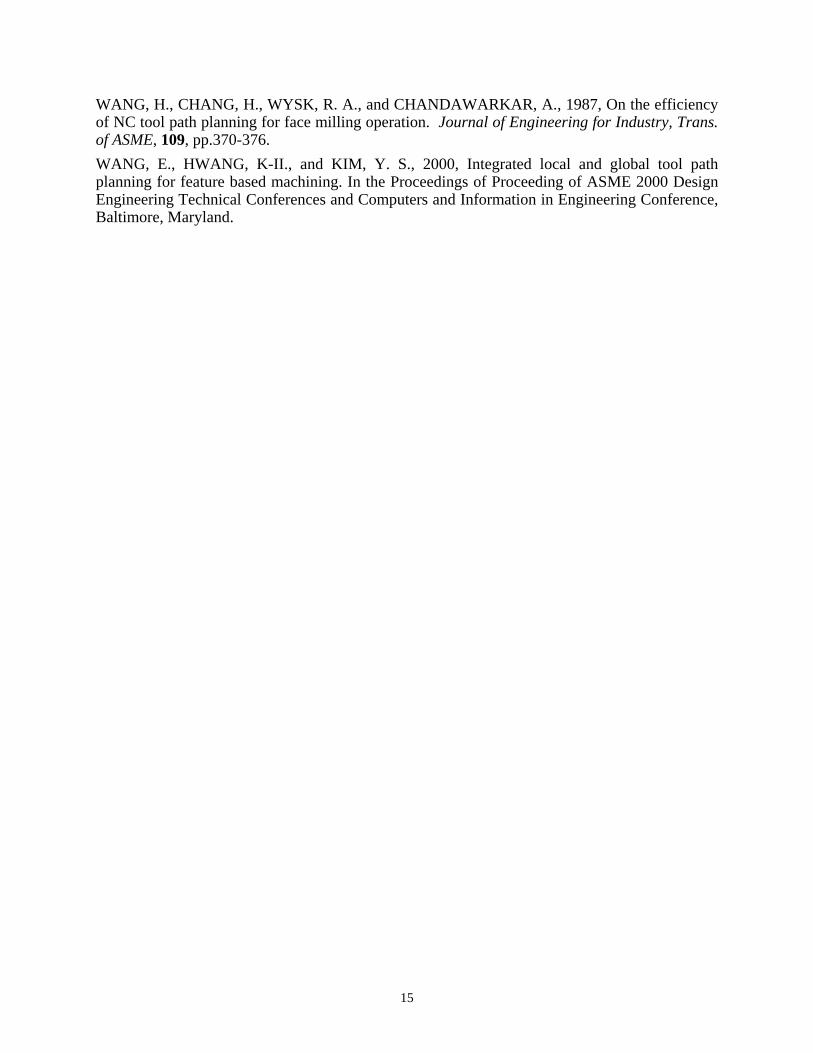
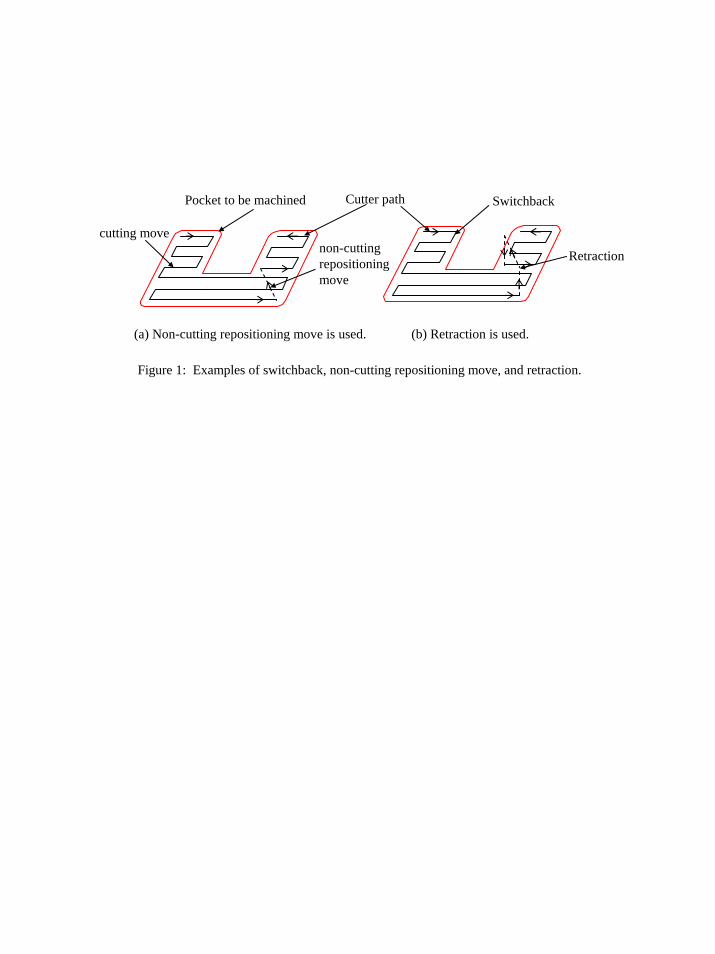
2.5D milling operation is a very common machining operation. Usually, there are two types of machining operations, i.e., rough machining and finish machining. In rough machining, raw material is removed as quickly as possible, whereas in finish machining, the surface finish and geometric accuracy are also given equal importance. A study shows that approximately 50% of total cutting time in mould and die manufacturing is spent in the rough cutting stage (Hatna et al. 1998). Therefore, finding efficient cutter paths for rough machining will enhance overall throughput of the manufacturing process. In the 2.5D milling process, cutter paths usually consist of three types of cutter movements as shown in figure 1: (1) the cutter engages with the material and performs cutting (i.e., cutting move); (2) the cutter moves at a feed rate as part of repositioning operation and does not engage in the cutting process (i.e., non-cutting repositioning move); (3) the cutter lifts up to a clearance height, moves to another position rapidly and then lowers down to perform another cutting motion (i.e., retraction). Among these three types of movement, the first one actually cuts the material, and usually consumes the majority of the machining time. The other two are used to link disconnected cutting moves together and thus increase the total machining time. Different cutter paths result in different cutting efficiencies, thus leading to different total cutting times. Cutting efficiency can be measured by cutting engagement (Kramer 1992). Cutter engagement is the percentage of the cutter that engages with the material while the cutter moves as shown in figure 2. Section 5.2

1 Corresponding Author

1

will describe the use of cutter engagement in computing cutter paths. One special case that results in low cutting efficiency is when the cutter makes sharp turns. The sharp turns consume longer time than ordinary cutting moves not only because the cutting engagement value is low, but also because the cutter has to slow down and then speed up when the cutting direction changes sharply. These sharp turns are called switchbacks. For traditional NC machining, the feed rate is relatively low, and hence the time spent on slowing down and speeding up in switchbacks can be ignored. However, for high speed machining, the number of switchbacks will influence the total cutting time significantly (Sarma 1999). Therefore, while generating a good cutter path, one should consider all these factors. Ideally, a good cutter path should have no retraction and non-cutting movement, the cutter engagement should be constant, and the cutting efficiency at every point along the cutter path should be high. In this paper, Section 3 describes two popular approaches for generating cutter paths, i.e., cutter paths based on predefined curves, and the emergent patterns based on grid traversing. Both approaches may not produce efficient cutter paths in certain cases. The reason behind this is as follows. For different types of pocket geometries, different cutter path patterns have shown to be efficient. However, in certain types of complex pockets, no single cutter path pattern produces efficient paths throughout the pocket. For complex pockets, a cutter path that combines different cutter path patterns (called hybrid patterns in this paper) is believed to lead to efficient cutting (Li et al. 1994, Hatna et al. 1998). One possible approach to generate hybrid patterns is to use heuristics to select the best cutter path pattern for different portions of a given feature. However, as described in Section 4, existing heuristics work only under certain conditions. A new algorithm is described in Section 5 for generating hybrid patterns. This algorithm generates cutter path by selecting different patterns in different regions of the feature and seamlessly morphing them together at the interface. This algorithm produces solutions at least as good as those produced by well-known single patterns. On the other hand in case of complex pockets, it produces solutions superior to those generated by any single pattern. 2 RELATED WORKS The cutter path planning area has been studied for a long time and has a vast literature. The following sections will only introduce techniques that are of direct relevance to the method described in this paper. For an overview of other work in the cutter path planning area, please refer to (Marshall and Griffiths 1994, Hatna et al. 1998, Sarma 2000). Wang and Chang (1987) did a systematic study in order to determine the factors affecting the efficiency of pocket milling operation, specifically the starting point, the cutting orientation and the cutter path generation algorithm. They carried out comprehensive experiments to compute the tool path length for various convex pockets from triangles to heptagons. They concluded that in zigzag milling, the cutting orientation affects the length of cut by 5-10 percent on an average, although in the worst case the variation can be as much as 100 percent. They came up with the rule of thumb that in the zigzag milling, the orientation parallel to the longest side of the polygon results in the optimum or near optimum cutter path length. As shown in Section 4, some of these heuristics may not always produce correct predictions. Wang, Hwang and Kim (2000) presented an integrated method for local and global tool path planning for feature based machining. Their algorithm has a feature recognition module that not only recognizes machining features from the solid model, but also determines the precedence of

2

features based on their geometry. Tool path for each machining feature is computed separately and then linked with each other to obtain the global tool path. For each feature, there can be multiple start and end point pairs. The global tool path is computed in such a way as to minimize the non-cutting movement of the tool. This determines the start and end point pair for each local feature. In their paper, they use contouring patterns to generate tool paths for local features. Bala and Chang (1991) have presented an algorithm for pocket milling that covers optimal tool selection and cutter path generation. Their algorithm selects the largest cutter capable of machining the entire pocket. Once an appropriate tool is chosen, the pocket is subdivided into different regions in which the tool can move without gouging the pocket boundaries. This is done by forming offset curves to the pocket boundary. Offset curves may intersect with each other to form loops. The algorithm decides which loops are to be covered and which are to be left. It also presents a way to join island-offset curves. After determining the feasible region of tool motion, the cutter path is generated using a zigzag pattern. The orientation of scan lines is chosen parallel to the longest edge of the pocket. In case of non-convex pockets, tool retractions may be needed. Jamil (1997) has presented an algorithm for milling non-convex pockets based on zigzag milling. Scan lines are parallel to one of the edges of the polygon. A search is made to determine the side along which machining will be done; the aim is to find the side that will not result in any tool retraction. The algorithm suggested for this search operation involves measuring the distance of all the vertices from a chosen reference side. If a vertex is closer to the reference side than either of it's adjacent vertices, then another side is chosen as the reference. This procedure is continued until a side that satisfies the above criteria is found. In case no such side exists, he suggests dividing the polygon, preferably by connecting two vertices. The algorithm requires two passes of contouring before the actual zigzag can start. Tang et al. (1998) have presented an algorithm based on zigzag milling to minimize the number of tool retractions for a pocket with holes and islands. The algorithm aims to find the optimum inclination of the sweep lines and the minimum number of partitions required for the pocket. The partitioning is done in such a way that no tool retraction is required within a sub-region. The partitioning is restricted such that it is parallel to the scan lines. This may result in a sub-optimum solution, but use of non-parallel partitioning may result in a very complex problem to analyse. The number of partitions for a pocket depends on the pocket geometry and the sweep angle. For a given sweep angle, there are several configurations in which a pocket can be divided. Each configuration has been considered separately and a few have been ruled out, as they may not be minimum. Others can be transformed into a particular configuration without increasing the number of total partitions. The algorithm to do this has also been presented. Choi and Park (2000) have presented an algorithm for zigzag pocket milling that determines the optimum inclination, calculates the cutter path segments, and links them. The principle behind determining the optimum inclination is to minimize the number of tool retractions. The algorithm captures the geometrical complexity of the pocket as well as the tool path interval. For the purpose of generating tool path segments, the authors have presented the concept of monotone chain and plane-sweep paradigm. The tool path-linking problem is dealt with separately for one-way and zigzag milling. In case of zigzag milling, the problem is modeled as tool-path element net traveling problem.

3

Kramer (1992) suggested the use of the knowledge of the amount of tool engagement in varying the feed rate and the spindle-speed, along the cutter path in order to reduce the cutting time. Sarma (1999) considered the switchbacks in zigzag milling to be a major contributor in the total machining time and has provided an algorithm to minimize it. Persson (1978) used bisector and trisector curves of pocket boundaries to generate the cutter path. Suh and Lee (1990) improved upon his algorithm by allowing free form curves to define the pocket boundary. Chou (1989) attempted to subdivide a non-convex pocket into convex one. The cutter path for each sub pocket was generated using contouring and then linked to each other by a heuristic solution similar to the solution of traveling salesman problem. Ferstenberg et al. (1986) suggested forming a tree of pocket boundaries to generate the cutter path for pocket milling. They treated star shaped pockets separately to generate cutter path. Deshmukh and Wong (1993) have studied the problem of uncut area in zigzag pocket milling of convex polygon. Thus we see that a lot of useful work has been done in the field of traditional zigzag machining aimed at minimizing the total number of tool retractions. However, to the best of our knowledge, a systematic study of generation of hybrid patterns for arbitrary shaped pockets has not been done. In the field of computational geometry, emergent patterns based on grid traversing have been widely studied. For a detailed description and related work, please refer to (Arkin et al. 2000). The grid-traversal problem has been shown to be NP hard (Arkin et al. 1993). Therefore, several approaches have been proposed using approximation algorithms (Arkin et al. 1996, Hochbaum 1997). For example, in (Arkin et al. 2001), an approximation algorithm is described with a 3.75-approximation for minimum-turn axis-parallel tours for a unit square cutter that covers an integral orthogonal polygon. In conclusion, if the feature shape is complex, a single cutter path pattern cannot generate efficient cutter path. Therefore, a new approach is needed that can be used to generate efficient cutter path for geometrically complex features. 3 ANALYSIS OF EXISTING CUTTER PATH PATTERNS

In 2.5D milling cutter path planning, two main types of cutter patterns are used. The first involves the use of patterns based on predefined curves and the second involves emergent patterns based on grid traversing. This section describes these two patterns. 3.1 Patterns Based on Predefined Curves

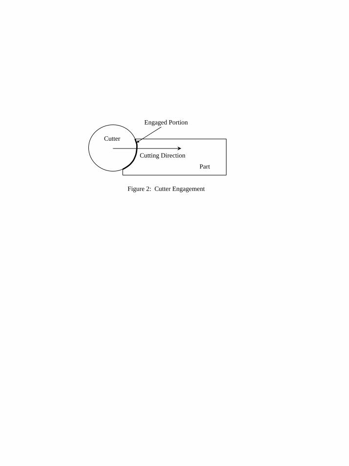
Patterns based on predefined curves use a series of predefined curves to cover the region to be cut. These predefined curve segments are called base curves. In most cases, additional cutter path segments are used to link these predefined curve segments together. These segments are called linkage segments. The most commonly used patterns in this category are zigzag and contour parallel. The patterns based on spiral curve and space filling curve approaches can also be included in this category. 3.1.1 Zigzag The general zigzag pattern refers to those methods that use a series of parallel open curve segments as the base curve to cover the pocket as shown in figure 3 (Sarma 2000). The base curve shape can be a straight line, a circular arc or even a portion of the boundary curve as

4

shown in figures 3 and 4. In order to link the base curves together, three types of linkage methods, i.e., zag, zigzag and modified zigzag are used as shown in figure 3 (Gupta et al. 2001). Different combinations of base curve shapes and linkage methods result in different cutter paths.

The merit of using straight line as a base curve lies in its computational efficiency. One may easily derive mathematical equations to calculate the intersection points of straight lines with a pocket boundary. Therefore, straight line based zigzag cutter path trajectory method is commonly used in practice. However, the staircase shape left by those line segments along the boundary of the pocket results in an uneven surface finish and uncut material. Therefore, usually a final contouring that cleans these scallops is needed. In some cases, circular curve based trajectory layout gives better cutter path than the straight line based method. Figure 4(a) shows such an example in which the boundary of the pockets is composed of a series of arcs. Although calculating the intersection points of those circular segments with the boundary is harder than those with straight lines, as shown in figure 3, the cutter path generated using this method is more efficient in these cases.

In some special cases such as the example shown in figure 4(b), both straight line and circular arc give inefficient cutter paths. The method that uses part of the pocket boundary curve generates more efficient cutter path. However, finding a proper base curve in this case is harder especially for generating cutter paths automatically. Zigzag method is used in most CAD/CAM software. Even though they are easier to generate, zigzag patterns sometime result in inefficient cutter paths. If the shape of the pocket becomes complex, a single orientation gives inefficient cutter path as shown in figure 3(d). However, one can also use several different inclinations within a pocket to obtain a more efficient cutter path as shown in figure 5. 3.1.2 Contour Parallel Contour parallel method uses a series of closed curves as base curves to cover a pocket. Extra cutter path segments are used to link these curves together. There are mainly two different types of closed curve: 1. The most commonly used is the contour parallel method that uses a series of offset curves of

the boundary to cover the pocket. Most published algorithms use Voronoi diagram to compute the offset curves.

2. Another method uses a series of window shape to cover a pocket. These window shapes are

either rectangular or circular. The computation is easy. However, it is hard to cover an irregular shape with full windows.

The contour parallel method is also used in CAD/CAM software. Although it involves more intense computations than the zigzag cutter path, in most cases it has a fewer number of switchbacks. However, for certain pocket shapes (as shown in figure 6), resulting cutter paths may be highly inefficient.

5

3.1.3 Spiral Curve Based and Space-filling Curve Based Spiral curve based trajectory layout does not require additional linkage cutter path segments. Therefore, in some cases it results in efficient cutter path. Moreover, this method allows the cutter to always cut some portion of the material, thus results in approximately constant engagement (Stori and Wright 2000). Maintaining constant cutter engagement gives better dynamic properties to cutting processes. However, constructing spiral curve based trajectory is computationally more intensive than contour parallel method. Therefore, spiral curve based cutter path is not as commonly used as zigzag and contour parallel cutter paths. A space-filling curve is defined as a continuous mapping of a unit line segment onto the unit square. Several types of space-filling curves exist based on the types of initiator and generator used to create the space-filling curve of any resolution. A space-filling curve based cutter path does not need additional linkage cutter path segment. However, it results in a large number of sharp corners. Hence the cutting efficiency is low and the surface finish is poor (Sarma 2000), thus, it is not commonly used. 3.2 Emergent Patterns Based on Grid Traversing Emergent patterns based on grid traversing are developed in the computational geometry community. Approaches in this category first represent a pocket by a grid, then find an optimal or near optimal tour that travels all grid points with minimal cost (for example, the length of the tour) using greedy algorithms. The rationale behind these approaches is as follows. Given a cutter and a pocket, finding the milling cutter path geometrically can be cast as the problem that finds a path or a tour whose Minkowski sum is the given pocket region. Therefore, if one can search all possible movements of the cutter, there should be an optimal solution. However, if the cutter can move along any direction as long as it does not touch the boundary, the search space is too large to be solved. In the computational geometry community, several efforts have been made to find an optimal tour by restricting the cutter movement directions. The most common approach is shown in figure 7. In this approach, the pocket is first decomposed into a grid. The size of the grid is determined by the cutter size. The cutter is considered to have a unit square shape and can move only vertically or horizontally. After that, a tour that covers the entire grid can be found. The grid-traversal problem has shown to be NP hard (Arkin et al. 1993). Therefore, several approaches based on approximation algorithms have been proposed. For example, in (Arkin et al. 2001), an approximation algorithm is given with a 3.75-approximation for minimum-turn axis-parallel tours for a unit square cutter that covers an integral orthogonal polygon. 3.3 Summary These two traditional cutter path patterns have their merits and drawbacks. The patterns based on predefined curves constrain the possible layouts of the cutter path, and thus may lead to inefficient cutter paths when the pocket geometry is not a natural match for these curves. The emergent patterns based on grid traversing solve the problem by constraining the possible cutter movements and possible cutter locations. Thus, although near-optimal cutter paths can be found in some cases, the approximation is not acceptable in many cases. Therefore, new methods that

6

take advantages of both these approaches and lead to hybrid patterns are required for handling geometrically complex features.

4 ANALYSES OF EXISTING HEURISTICS

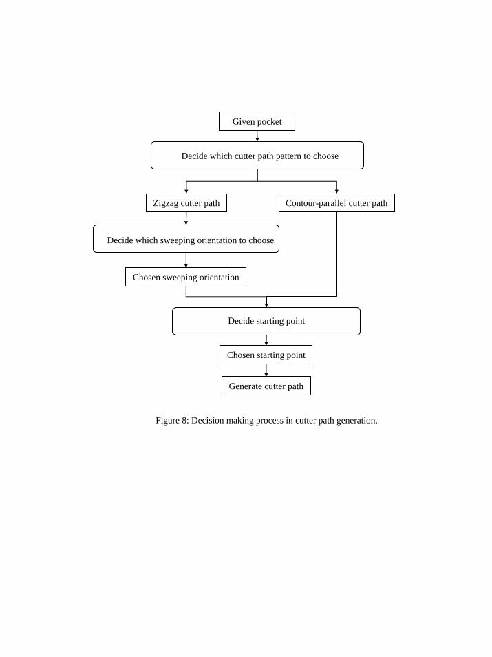
One possible approach is to use heuristics to select the best cutter path pattern for each portion of a given feature. However, in order to use this approach, the following questions need to be answered: Are there any heuristics? Are these heuristics valid? And when are they valid? This section shows a few of the existing heuristics. Figure 8 shows the decision making process in generating the cutter path for a complex feature. First of all, users should select which cutting pattern to choose. If zigzag is selected, then users should first select a sweeping direction, and then select a starting point to generate the zigzag cutter path. On the other hand, if contour-parallel is selected, then users only need to select a starting point in order to get the cutter path. Therefore, three decisions should be made in this process. The following section shows existing heuristics for these three decision-making steps. 4.1 Heuristics for Pattern Selection

The first step is to decide which cutter path pattern to use. This paper only includes two commonly used patterns, i.e., zigzag and contour-parallel. The heuristic in existing literatures states that: For regular shapes, zigzag is more efficient, however for complex shapes, the contour is more efficient (Hatna et al. 1998). This heuristic does not precisely define what “regular” and “complex” mean. The rationale behind this heuristic may be that for complex shapes, generating zigzag cutter path may lead to more disconnected cutter path segments, thus need more retractions. However, for complex shapes, contour-parallel sometimes results in inefficient loops and hence poor cutter paths. On the other hand, for a “regular” shape as shown in figure 9, contour-parallel pattern results in a better cutter path than zigzag. Moreover, for a “complex” shape as shown in figure 10, zigzag produces a better cutter path. Therefore, this heuristic offers limited help in making a decision at this step. 4.2 Heuristics for Sweeping Direction Selection

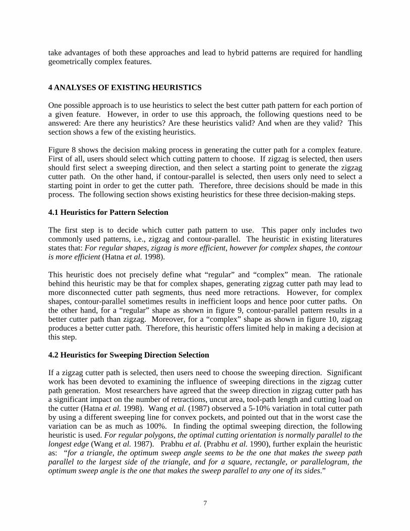
If a zigzag cutter path is selected, then users need to choose the sweeping direction. Significant work has been devoted to examining the influence of sweeping directions in the zigzag cutter path generation. Most researchers have agreed that the sweep direction in zigzag cutter path has a significant impact on the number of retractions, uncut area, tool-path length and cutting load on the cutter (Hatna et al. 1998). Wang et al. (1987) observed a 5-10% variation in total cutter path by using a different sweeping line for convex pockets, and pointed out that in the worst case the variation can be as much as 100%. In finding the optimal sweeping direction, the following heuristic is used. For regular polygons, the optimal cutting orientation is normally parallel to the longest edge (Wang et al. 1987). Prabhu et al. (Prabhu et al. 1990), further explain the heuristic as: “for a triangle, the optimum sweep angle seems to be the one that makes the sweep path parallel to the largest side of the triangle, and for a square, rectangle, or parallelogram, the optimum sweep angle is the one that makes the sweep parallel to any one of its sides.”

7

The sweeping direction influences the zigzag cutter path due to the following reasons: 1. Variation of linkage segments results in total cutter path length changes. Total cutter path

length includes parallel cutter path segments, along which cutter removes material, as well as linkage segments. The number of real cutting segments along any orientation should approximately be constant because the area formed by the swept region of these segments should be approximately equal to the area to be cut. However, one of the reasons that cause different orientations to give different total cutter path is that linkage segments are different. The total length of these linkage segments can be estimated as (L(B)-L(S))/2. In the formula, L(B) is the length of the boundary, L(S) is the length of the boundary segment that is parallel to the cutter path orientation. Therefore, if the longest boundary side is selected as the sweeping direction, then the total length of linkage segments is minimum.

2. Variation of starting and ending cutter path segments gives different total cutter path length

for some cases. To machine a convex pocket using the zigzag pattern, the sweeping direction along the longest edge seems to give the shortest cutter path length. This is based on the observation that the last cutter path segment often does not machine the pocket as efficiently as the remaining segments. This happens because the distance between the lowest and the highest points in the pocket is rarely an integral multiple of tool step size. Hence, in the final cut, the tool step-over distance is usually smaller than in other cuts, resulting in inefficient cutting and a longer cutter path (e.g., figure 11). If the sweeping orientation is chosen along the longest edge, then the last segment is likely to be relatively small. Hence the length of the inefficient cut will be shorter.

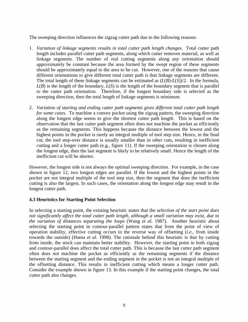
However, the longest side is not always the optimal sweeping direction. For example, in the case shown in figure 12, two longest edges are parallel. If the lowest and the highest points in the pocket are not integral multiple of the tool step size, then the segment that does the inefficient cutting is also the largest. In such cases, the orientation along the longest edge may result in the longest cutter path. 4.3 Heuristics for Starting Point Selection

In selecting a starting point, the existing heuristic states that the selection of the start point does not significantly affect the total cutter path length, although a small variation may exist, due to the variation of distances separating the loops (Wang et al. 1987). Another heuristic about selecting the starting point in contour-parallel pattern states that from the point of view of operation stability, effective cutting occurs in the reverse way of offsetting (i.e., from inside towards the outside) (Hatna et al. 1998). The rationale behind this heuristic is that by cutting from inside, the stock can maintain better stability. However, the starting point in both zigzag and contour-parallel does affect the total cutter path. This is because the last cutter path segment often does not machine the pocket as efficiently as the remaining segments if the distance between the starting segment and the ending segment in the pocket is not an integral multiple of the offsetting distance. This results in inefficient cutting which means a longer cutter path. Consider the example shown in figure 13. In this example if the starting point changes, the total cutter path also changes.

8

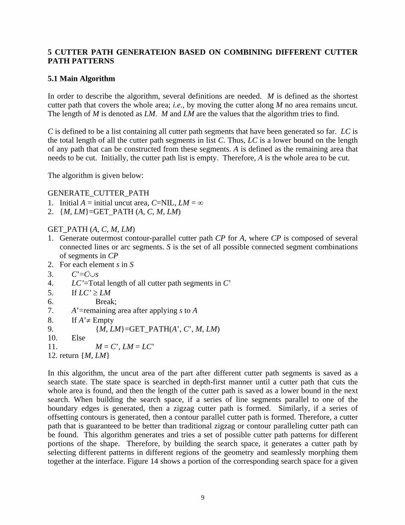
5 CUTTER PATH GENERATEION BASED ON COMBINING DIFFERENT CUTTER PATH PATTERNS 5.1 Main Algorithm In order to describe the algorithm, several definitions are needed. M is defined as the shortest cutter path that covers the whole area; i.e., by moving the cutter along M no area remains uncut. The length of M is denoted as LM. M and LM are the values that the algorithm tries to find. C is defined to be a list containing all cutter path segments that have been generated so far. LC is the total length of all the cutter path segments in list C. Thus, LC is a lower bound on the length of any path that can be constructed from these segments. A is defined as the remaining area that needs to be cut. Initially, the cutter path list is empty. Therefore, A is the whole area to be cut. The algorithm is given below: GENERATE_CUTTER_PATH 1. Initial A = initial uncut area, C=NIL, LM = ∞ 2. {M, LM}=GET_PATH (A, C, M, LM) GET_PATH (A, C, M, LM) 1. Generate outermost contour-parallel cutter path CP for A, where CP is composed of several

connected lines or arc segments. S is the set of all possible connected segment combinations of segments in CP

2. For each element s in S 3. C’=C∪s 4. LC’=Total length of all cutter path segments in C’ 5. If LC’ ≥ LM 6. Break; 7. A’=remaining area after applying s to A 8. If A’≠ Empty 9. {M, LM}=GET_PATH(A’, C’, M, LM) 10. Else 11. M = C’, LM = LC’ 12. return {M, LM} In this algorithm, the uncut area of the part after different cutter path segments is saved as a search state. The state space is searched in depth-first manner until a cutter path that cuts the whole area is found, and then the length of the cutter path is saved as a lower bound in the next search. When building the search space, if a series of line segments parallel to one of the boundary edges is generated, then a zigzag cutter path is formed. Similarly, if a series of offsetting contours is generated, then a contour parallel cutter path is formed. Therefore, a cutter path that is guaranteed to be better than traditional zigzag or contour paralleling cutter path can be found. This algorithm generates and tries a set of possible cutter path patterns for different portions of the shape. Therefore, by building the search space, it generates a cutter path by selecting different patterns in different regions of the geometry and seamlessly morphing them together at the interface. Figure 14 shows a portion of the corresponding search space for a given

9

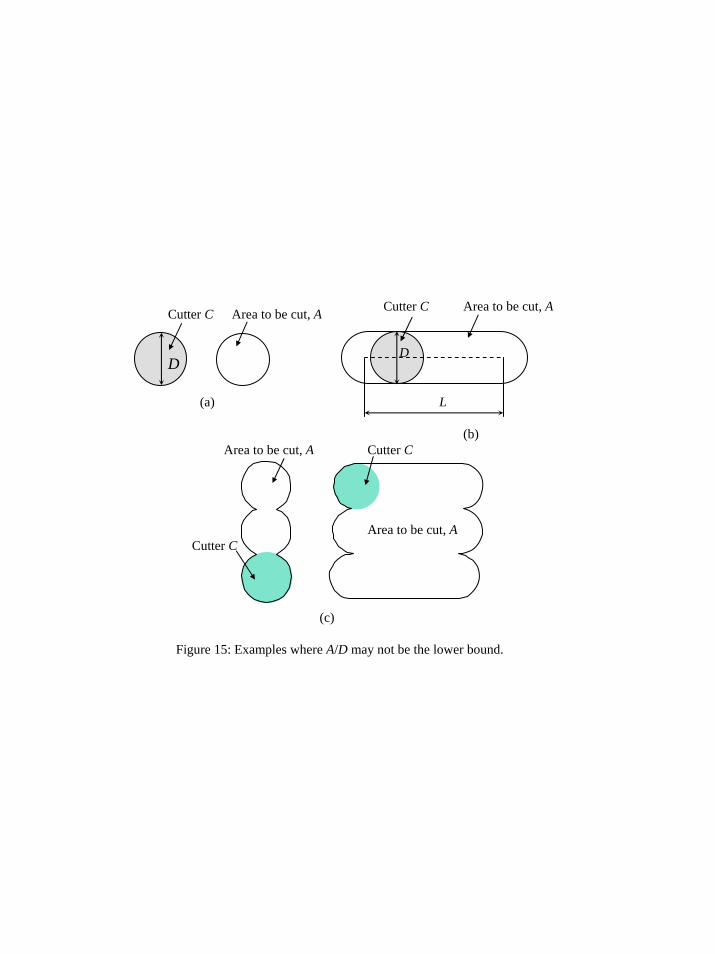
pocket. After all cutter path segments are finalized, these segments are linked together using an algorithm similar to the one described by Park and Choi (2000). We use a standard depth-first branch and bound search algorithm. For this kind of algorithms, the running time in the worst case could be exponential. However, with the help of pruning heuristics described in Section 5.2, the algorithm prunes a large portion of search space. Thus, it works in a computationally efficient manner. 5.2 Heuristics Used in the Algorithm In Step 6 of algorithm GET_PATH, the search will stop if the currently expanded cutter path C’ is longer than the shortest total cutter path M found so far. This step will prune some branches in the search space. Furthermore, at one particular state, the remaining area A' can be obtained by performing Boolean operations using the currently expended cutter path. If the lower bound of the length of the cutter paths that can cover A' (say LB) can be found, then the result of LB BB + LC' can be used to estimate the lower bound of the total length of this search branch. Thus the following forward-looking heuristic can be used: If LB + LB C' > LM, then stop expending the current search node. This heuristic can prune additional branches. The key in this heuristic is to find a feasible lower bound. Given a cutter with diameter D, and an area A to be cut, the commonly used equation in estimating the lower bound of cutter path length is LB = A/D. However, can this equation produce a feasible lower bound? In other word, is it true that for any given shape A, there is no way one can generate a cutter path that can cover A such that its length is less than A/D?

B

In order to answer this question, the following cases are examined: 1. Figure 15(a) shows an example where A is exactly the same as the area a cutter can cut when

the cutter is located at the center of A. In this case, the total cutter path length is 0 and A/D = (π (D/2)2)/D = πD/4 > 0.

2. Figure 15(b) shows another example, where the cutter path length is L, and the area cut by

the cutter is A = LD + π (D/2)2. In this case, A/D is geometrically not the lower bound. A more accurate estimate is obtained by using the equation: LB = (A - π (D/2) )/D. B

2

3. Figure 15(c) shows two other examples. In these cases, there will be large errors if A/D is

used as lower bound. In these examples, it appears that portions of the area (those half circular regions) are cut without moving the cutter, i.e., with 0 length cutter path. However, in practice, these areas are cut by plunging the cutter into the material. Therefore, when considering total cutter path length, the cutter path length for those half circular regions cannot be 0. Usually, the feed rate for plunging in the cutter is much slower than the normal feed rate. Therefore, suppose the plunging in feed rate is α1, and the normal feed rate is α2, and the depth of cut is d, then the plunging in movement should be converted into a normal cuter path length L’ by: L’ = da2/a1. Therefore, practically, for the example shown in figure 15(b), the real lower bound should be:

10

2

2 2

1 1

24B

DAd dA DL

D D

πα α πα α

⎛ ⎞− ⎜ ⎟⎝ ⎠= + = + −

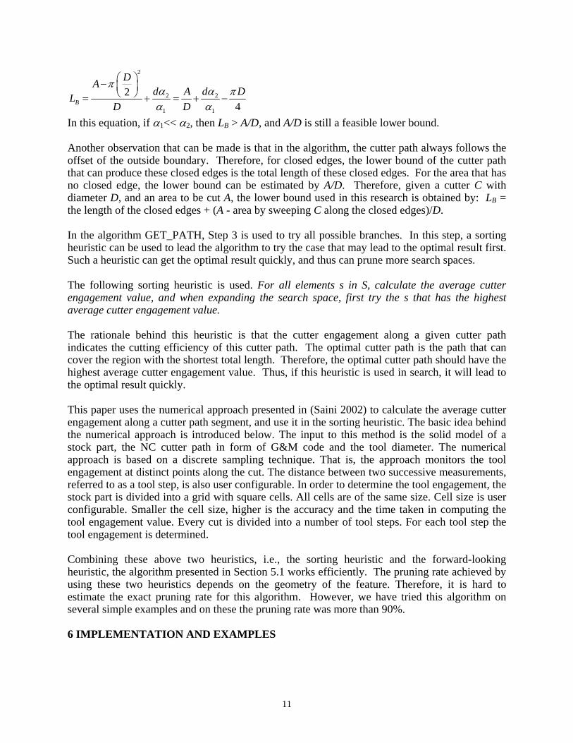
In this equation, if α1<< α2, then LB > A/D, and A/D is still a feasible lower bound. B

Another observation that can be made is that in the algorithm, the cutter path always follows the offset of the outside boundary. Therefore, for closed edges, the lower bound of the cutter path that can produce these closed edges is the total length of these closed edges. For the area that has no closed edge, the lower bound can be estimated by A/D. Therefore, given a cutter C with diameter D, and an area to be cut A, the lower bound used in this research is obtained by: LB = the length of the closed edges + (A - area by sweeping C along the closed edges)/D.

B

In the algorithm GET_PATH, Step 3 is used to try all possible branches. In this step, a sorting heuristic can be used to lead the algorithm to try the case that may lead to the optimal result first. Such a heuristic can get the optimal result quickly, and thus can prune more search spaces. The following sorting heuristic is used. For all elements s in S, calculate the average cutter engagement value, and when expanding the search space, first try the s that has the highest average cutter engagement value. The rationale behind this heuristic is that the cutter engagement along a given cutter path indicates the cutting efficiency of this cutter path. The optimal cutter path is the path that can cover the region with the shortest total length. Therefore, the optimal cutter path should have the highest average cutter engagement value. Thus, if this heuristic is used in search, it will lead to the optimal result quickly. This paper uses the numerical approach presented in (Saini 2002) to calculate the average cutter engagement along a cutter path segment, and use it in the sorting heuristic. The basic idea behind the numerical approach is introduced below. The input to this method is the solid model of a stock part, the NC cutter path in form of G&M code and the tool diameter. The numerical approach is based on a discrete sampling technique. That is, the approach monitors the tool engagement at distinct points along the cut. The distance between two successive measurements, referred to as a tool step, is also user configurable. In order to determine the tool engagement, the stock part is divided into a grid with square cells. All cells are of the same size. Cell size is user configurable. Smaller the cell size, higher is the accuracy and the time taken in computing the tool engagement value. Every cut is divided into a number of tool steps. For each tool step the tool engagement is determined. Combining these above two heuristics, i.e., the sorting heuristic and the forward-looking heuristic, the algorithm presented in Section 5.1 works efficiently. The pruning rate achieved by using these two heuristics depends on the geometry of the feature. Therefore, it is hard to estimate the exact pruning rate for this algorithm. However, we have tried this algorithm on several simple examples and on these the pruning rate was more than 90%. 6 IMPLEMENTATION AND EXAMPLES

11

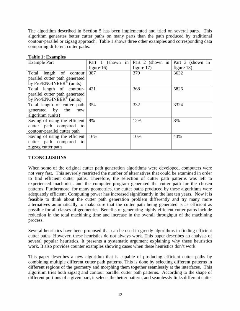
The algorithm described in Section 5 has been implemented and tried on several parts. This algorithm generates better cutter paths on many parts than the path produced by traditional contour-parallel or zigzag approach. Table 1 shows three other examples and corresponding data comparing different cutter paths. Table 1: Examples Example Part Part 1 (shown in

figure 16) Part 2 (shown in figure 17)

Part 3 (shown in figure 18)

Total length of contour parallel cutter path generated by Pro/ENGINEER® (units)

387 379 3632

Total length of contour-parallel cutter path generated by Pro/ENGINEER® (units)

421 368 5826

Total length of cutter path generated by the new algorithm (units)

354 332 3324

Saving of using the efficient cutter path compared to contour-parallel cutter path

9% 12% 8%

Saving of using the efficient cutter path compared to zigzag cutter path

16% 10% 43%

7 CONCLUSIONS When some of the original cutter path generation algorithms were developed, computers were not very fast. This severely restricted the number of alternatives that could be examined in order to find efficient cutter paths. Therefore, the selection of cutter path patterns was left to experienced machinists and the computer program generated the cutter path for the chosen patterns. Furthermore, for many geometries, the cutter paths produced by these algorithms were adequately efficient. Computing power has increased significantly in the last ten years. Now it is feasible to think about the cutter path generation problem differently and try many more alternatives automatically to make sure that the cutter path being generated is as efficient as possible for all classes of geometries. Benefits of generating highly efficient cutter paths include reduction in the total machining time and increase in the overall throughput of the machining process. Several heuristics have been proposed that can be used in greedy algorithms in finding efficient cutter paths. However, these heuristics do not always work. This paper describes an analysis of several popular heuristics. It presents a systematic argument explaining why these heuristics work. It also provides counter examples showing cases when these heuristics don’t work. This paper describes a new algorithm that is capable of producing efficient cutter paths by combining multiple different cutter path patterns. This is done by selecting different patterns in different regions of the geometry and morphing them together seamlessly at the interfaces. This algorithm tries both zigzag and contour parallel cutter path patterns. According to the shape of different portions of a given part, it selects the better pattern, and seamlessly links different cutter

12

path patterns together. Thus some portions of the final cutter path follow a zigzag pattern, and some other portions follow a contour parallel pattern. By using several examples, this paper shows that the new algorithm can lead to improved cutter paths in the case of complex geometries. Reduction in cutter path lengths ranges from 10% to 40% in the three examples presented in this paper. Since this algorithm examines many different solutions, and morphs cutter path generation patterns based on different geometrical shapes, it produces solutions at least as good as those produced by well-known single patterns. On the other hand in complex cases, it might produce solutions significantly superior to those generated by a single pattern. Therefore, as long as computational speed is not a bottleneck, combining multiple different cutter path patterns seems to be a logical solution. Most machine shops either already have or are likely to acquire a reasonably fast PC. So spending a few minutes on generating an efficient cutter path seems to be a reasonable course of action for these machine shops. Usually generating the zigzag cutter path for a pocket with 50 edges takes a fraction of a second on a fast PC. Therefore, in five minutes, several hundred combinations can be tried using a search algorithm. The algorithm described in this paper provides a first step towards generating efficient cutter paths. Currently, only a limited number of search heuristics are examined. In future, several more heuristics need to be explored to further improve the efficiency of this algorithm. Furthermore, only the shortest cutter path found so far is used as the lower bound, in the future, tighter bounds will need to be developed to enhance the performance of this algorithm. Acknowledgement. This research has been supported by NSF grant DMI0093142 and ONR grant N000140010416. Opinions expressed in this paper are those of authors and do not necessarily reflect opinion of the sponsors.

REFERENCES ARKIN, E. M., FEKETE, S. P., and MITCHELL, J. S. B, 1993, The lawnmower problem. In Proc. 5th Canad. Conf. on Computational Geometry, Waterloo, Ontario. ARKIN, E. M., HELD, M., and SMITH, C. L., 1996, Optimization problems related to zigzag pocket machining. In Proc. 7th ACM-SIAM Sympos. Discrete Algorithms, pp.419-428. ARKIN, E. M., HELD, M., and SMITH, C. L., 2000, Optimization problems related to zigzag pocket machining. Algorithmica, 26(2), pp.197--236. ARKIN, E. M., BENDER, M. A., DEMAINE, E. D., FEKETE, S. P., MITCHELL, J. S. B., and SETHIA, S., 2001, Optimal covering tours with turn costs. In Proc. 12th ACM-SIAM Sympos, Discrete Algorithms (SODA'2001). BALA, M., and CHANG, T. C., 1991, Automatic cutter selection and optimal cutter-path generation for prismatic parts. International Journal of Production Research, 29(11), pp. 2163-2176. CHOU, J. J., 1989, Numerical Control Milling Machine Tool Path Generation For Regions Bounded By Free-Form Curves And Surfaces, Ph.D. thesis, University of Utah. DESHMUKH, A., and WANG, H., 1993, Tool path planning for NC milling of convex polygonal faces: minimization of non-cutting area. Int. J. Adv. Manuf. Technol., 8(1), pp. 17-24.

13

FERSTENBERG, R. A., WANG, K. K., and MUCKSTADT, J., 1986, Automatic generation of optimized 3-axis NC programs using boundary files. IEEE International Conference on Robotics and Automation, pp. 325-332. GUPTA, S. K., SAINI, S. K., and YAO, Z., 2001, A geometric algorithm to generate efficient cutter path for complex pocket milling operation. In the Proceedings of ASME 2001 Computers and Information in Engineering Conference, Pittsburgh, Pennsylvania. HATNA, A., GRIEVE, R. J., and BROOMHEAD, P., 1998, Automatic CNC milling of pockets: geometric and technological issues. Computer Integrated Manufacturing Systems, 11(4), pp. 309-330. HOCHBAUM, D. S., 1997, Approximation Algorithms for NP-Hard Problems (PWS Publishing Company, Boston, MA). JAMIL, T. M., 1997, A computerized algorithm for milling non-convex pockets with numerically controlled machines. International Journal of Production Research, 35(7), pp.1843-1855. KRAMER, T. R., 1992, Pocket milling with tool engagement detection. Journal of Manufacturing Systems, 11(2), pp.114-123. LI, H., DONG, Z., and VICKERS, G. W., 1994, Optimal tool path pattern identification for single island, sculptured part rough machining using fuzzy pattern analysis. Computer Aided Design, 26(11), pp.787-795. MARSHALL, S., and GRIFFITHS, G. J., 1994, A survey of cutter-path construction techniques for milling machines. International Journal of Production Research, 32(12), pp.2861-2877. PARK, S. C., and CHOI, B. K., 2000, Tool-path planning for direction-parallel area milling. Computer Aided Design, 32(1), pp.17-25. PERSSON, H., 1978, NC machining of arbitrary shaped pockets. Computer Aided Design, 10(3), pp. 169-174. PRABHU, P.V., GRAMOPADHYE, A.K., and WANG, H. P., A general mathematical model for optimizing NC tool path for face milling of flat convex polygonal surfaces. International Journal of Production Research, 28(1), 1990, pp.101-130. SAINI, S. K., 2002, Algorithms for Computing Cutter Engagement in 2.5D Milling Operation, MS thesis, University of Maryland, College Park. SARMA, S. E., 1999, The crossing function and its application to zigzag tool paths. Computer Aided Design, 31(14), pp. 881-890. SARMA, R. 2000, An assessment of geometric methods in trajectory synthesis for shape creating operations. Journal of Manufacturing Systems, 19(1), pp. 59-72. STORI, J.A., and WRIGHT, P. K., 2000, Constant engagement tool path generation for convex geometries. Journal of Manufacturing Systems, 19(3), pp.172-184. SUH, Y. S., and LEE, K., 1990, NC milling tool path generation for arbitrary pockets defined by sculptured surfaces. Computer Aided Design, 22(5), pp. 273-284. TANG, K., CHOU, S. Y., and CHEN, L. L., 1998, An algorithm for reducing tool retractions in zigzag pocket machining. Computer Aided Design, 30(2), pp. 123-129.

14

WANG, H., CHANG, H., WYSK, R. A., and CHANDAWARKAR, A., 1987, On the efficiency of NC tool path planning for face milling operation. Journal of Engineering for Industry, Trans. of ASME, 109, pp.370-376. WANG, E., HWANG, K-II., and KIM, Y. S., 2000, Integrated local and global tool path planning for feature based machining. In the Proceedings of Proceeding of ASME 2000 Design Engineering Technical Conferences and Computers and Information in Engineering Conference, Baltimore, Maryland.

15

(a) Non-cutting repositioning move is used. (b) Retraction is used.

Figure 1: Examples of switchback, non-cutting repositioning move, and retraction.

Pocket to be machined SwitchbackCutter path

cutting movenon-cutting repositioning move

Retraction

Cutter

Cutting Direction

Part

Engaged Portion

Figure 2: Cutter Engagement

(a) Using straight lines to do intersection. (b) straight lines are base curves.

(c) Using zag method to link those base curves.

(d) Using zigzag method tolink those base curves.

(e) Using modified zigzag method to link those base curves.

Figure 3: Examples of different linkage methods by using straight line as base curve.

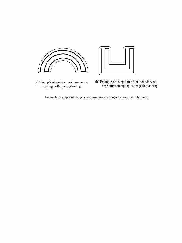
(a) Example of using arc as base curve in zigzag cutter path planning.

(b) Example of using part of the boundary asbase curve in zigzag cutter path planning.

Figure 4: Example of using other base curve in zigzag cutter path planning.

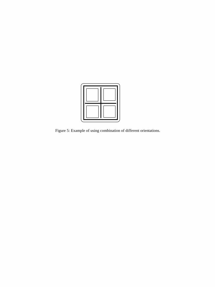
Figure 5: Example of using combination of different orientations.

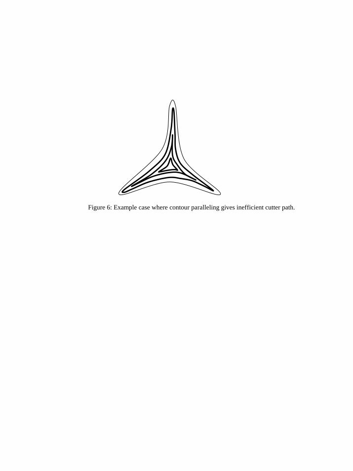
Figure 6: Example case where contour paralleling gives inefficient cutter path.

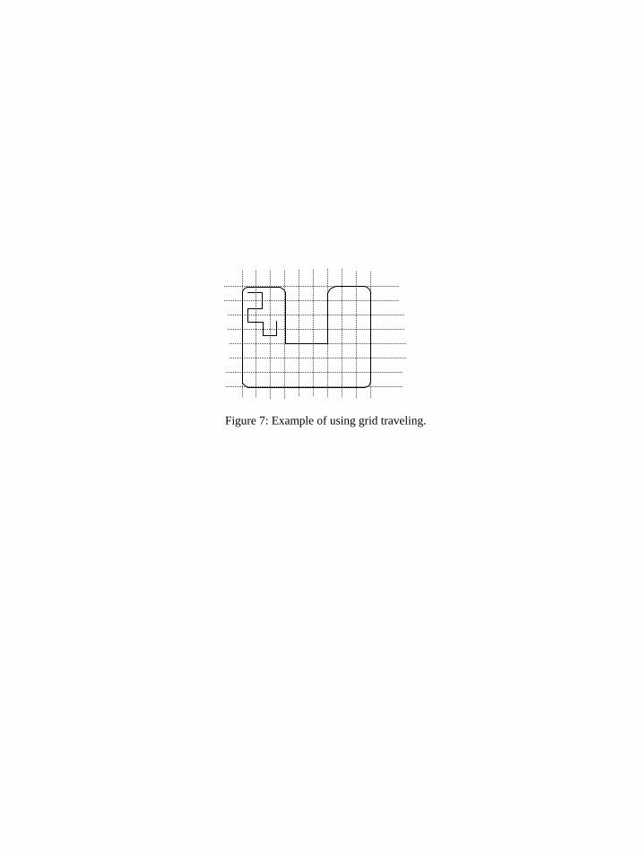
Figure 7: Example of using grid traveling.

Given pocket

Decide which cutter path pattern to choose

Decide which sweeping orientation to choose

Zigzag cutter path Contour-parallel cutter path

Chosen sweeping orientation

Decide starting point

Chosen starting point

Generate cutter path

Figure 8: Decision making process in cutter path generation.

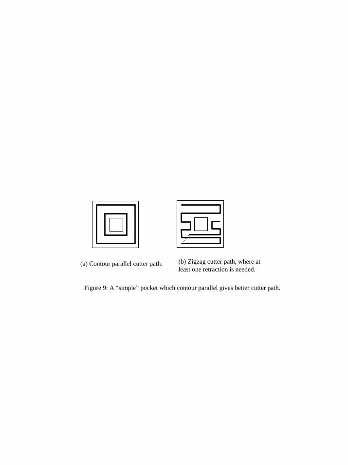
(a) Contour parallel cutter path. (b) Zigzag cutter path, where at least one retraction is needed.

Figure 9: A “simple” pocket which contour parallel gives better cutter path.

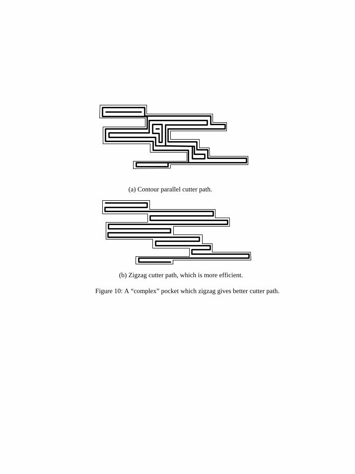
(a) Contour parallel cutter path.

(b) Zigzag cutter path, which is more efficient.

Figure 10: A “complex” pocket which zigzag gives better cutter path.

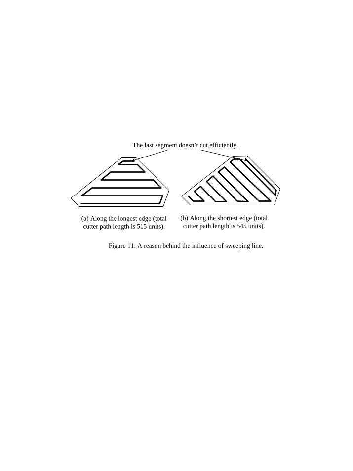
Figure 11: A reason behind the influence of sweeping line.

(a) Along the longest edge (total cutter path length is 515 units).

(b) Along the shortest edge (total cutter path length is 545 units).

The last segment doesn’t cut efficiently.

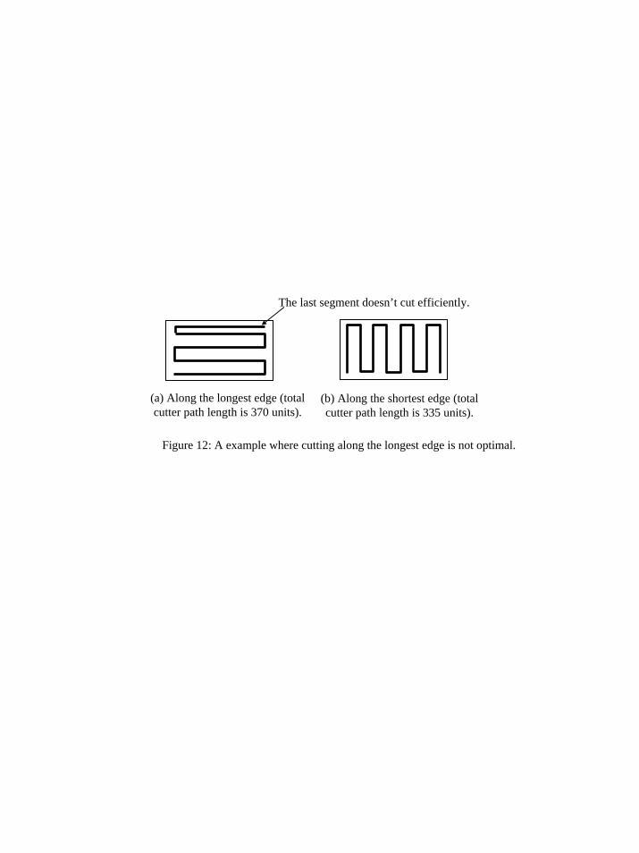
Figure 12: A example where cutting along the longest edge is not optimal.

(a) Along the longest edge (total cutter path length is 370 units).

(b) Along the shortest edge (total cutter path length is 335 units).

The last segment doesn’t cut efficiently.

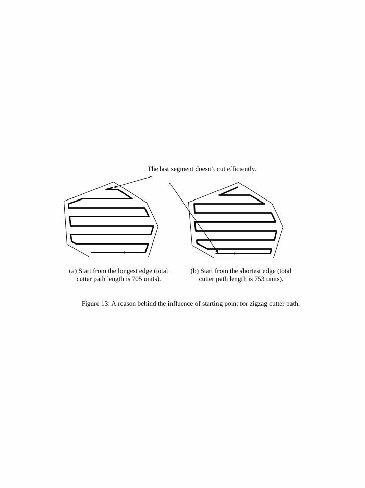
(a) Start from the longest edge (total cutter path length is 705 units).

(b) Start from the shortest edge (total cutter path length is 753 units).

The last segment doesn’t cut efficiently.

Figure 13: A reason behind the influence of starting point for zigzag cutter path.

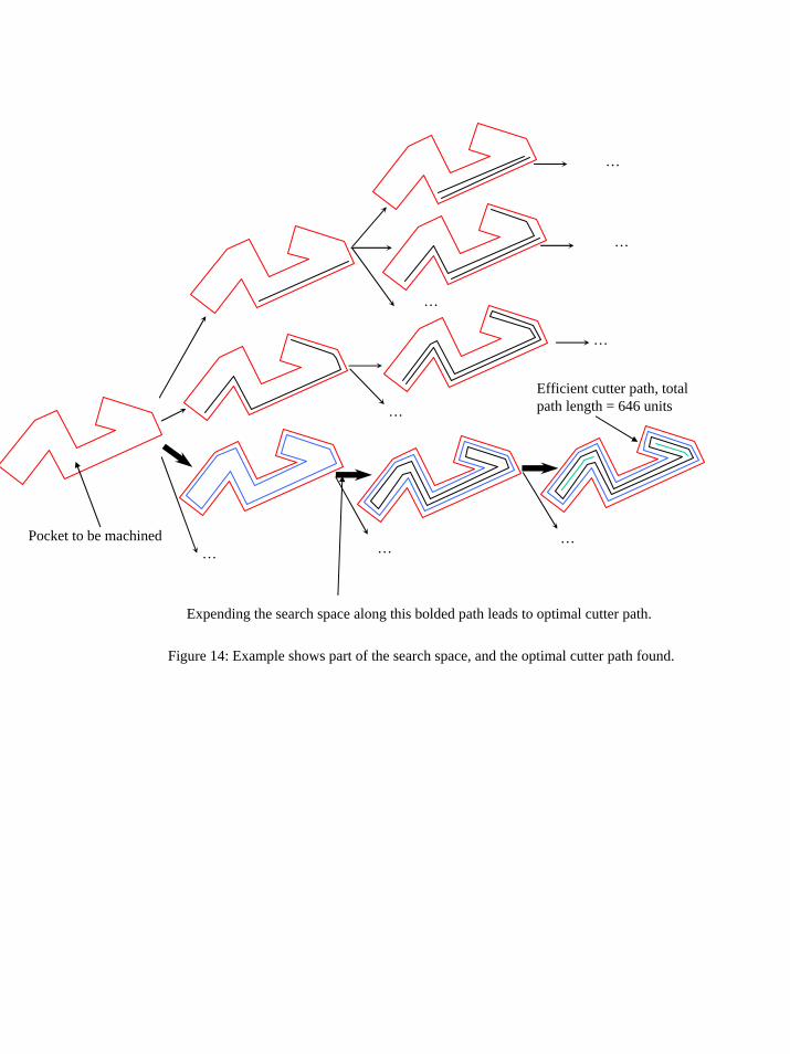
Figure 14: Example shows part of the search space, and the optimal cutter path found.

Pocket to be machined

Efficient cutter path, total path length = 646 units

… …

…

…

…

…

…

…

Expending the search space along this bolded path leads to optimal cutter path.

Cutter C Area to be cut, A

D

(a)

Cutter C Area to be cut, A

L

D

(b)

Cutter C Area to be cut, A

Area to be cut, A Cutter C

(c)

Figure 15: Examples where A/D may not be the lower bound.

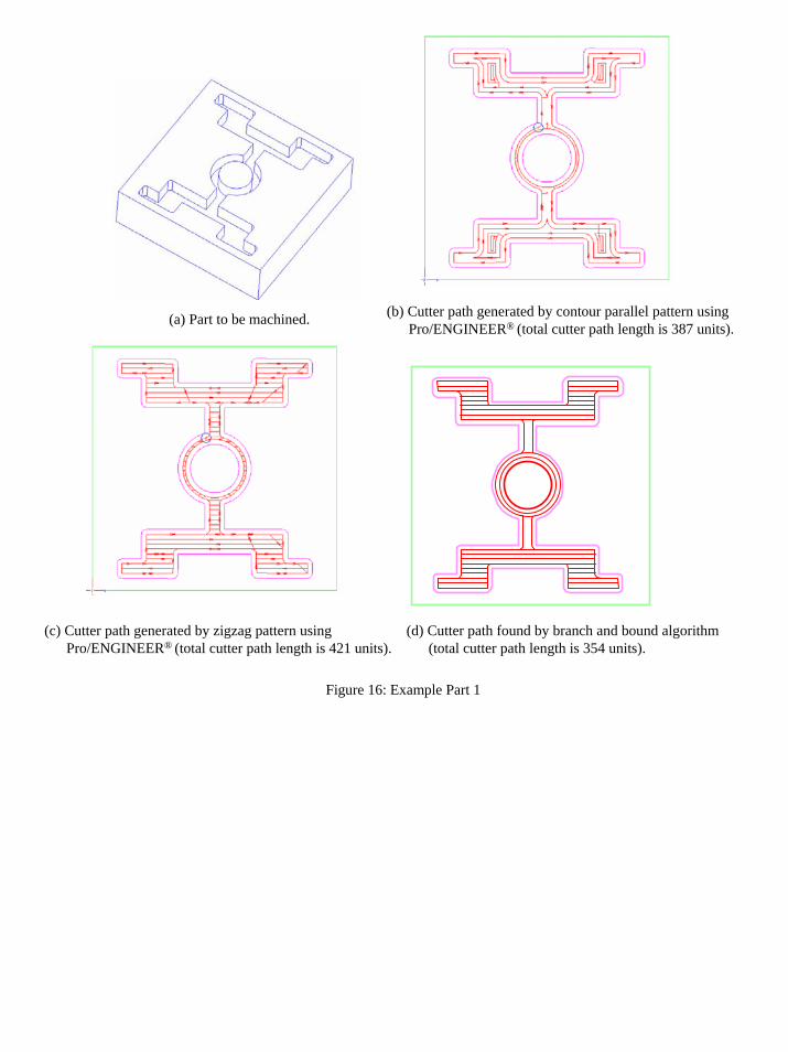
Figure 16: Example Part 1

(a) Part to be machined. (b) Cutter path generated by contour parallel pattern using Pro/ENGINEER® (total cutter path length is 387 units).

(c) Cutter path generated by zigzag pattern using Pro/ENGINEER® (total cutter path length is 421 units).

(d) Cutter path found by branch and bound algorithm (total cutter path length is 354 units).

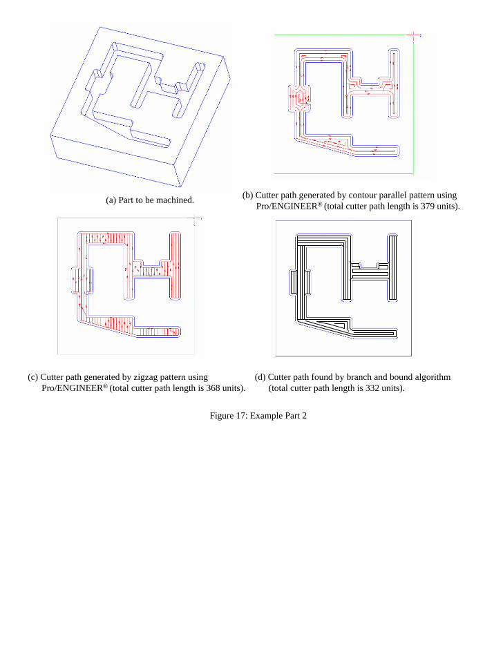
(a) Part to be machined. (b) Cutter path generated by contour parallel pattern using Pro/ENGINEER® (total cutter path length is 379 units).

(c) Cutter path generated by zigzag pattern using Pro/ENGINEER® (total cutter path length is 368 units).

(d) Cutter path found by branch and bound algorithm (total cutter path length is 332 units).

Figure 17: Example Part 2

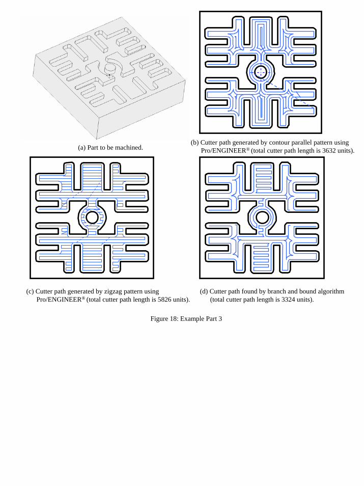
Figure 18: Example Part 3

(a) Part to be machined.(b) Cutter path generated by contour parallel pattern using

Pro/ENGINEER® (total cutter path length is 3632 units).

(c) Cutter path generated by zigzag pattern using Pro/ENGINEER® (total cutter path length is 5826 units).

(d) Cutter path found by branch and bound algorithm (total cutter path length is 3324 units).