Cutting Corners: Workbench Automation for Server Benchmarking · Cutting Corners: Workbench Automation for Server Benchmarking ... availability of hardware resources, deadlines, and

Cutting Corners: Workbench Automation

for Server Benchmarking

Piyush Shivam† Varun Marupadi+ Jeff Chase+ Thileepan Subramaniam+ Shivnath Babu+

†Sun Microsystems

[email protected]

+Duke University

{varun,chase,thilee,shivnath}@cs.duke.edu

Abstract

A common approach to benchmarking a server is to

measure its behavior under load from a workload gen-

erator. Often a set of such experiments is required—

perhaps with different server configurations or workload

parameters—to obtain a statistically sound result for a

given benchmarking objective.

This paper explores a framework and policies to con-

duct such benchmarking activities automatically and ef-

ficiently. The workbench automation framework is de-

signed to be independent of the underlying benchmark

harness, including the server implementation, configura-

tion tools, and workload generator. Rather, we take those

mechanisms as given and focus on automation policies

within the framework.

As a motivating example we focus on rating the peak

load of an NFS file server for a given set of workload

parameters, a common and costly activity in the storage

server industry. Experimental results show how an auto-

mated workbench controller can plan and coordinate the

benchmark runs to obtain a result with a target threshold

of confidence and accuracy at lower cost than scripted

approaches that are commonly practiced. In more com-

plex benchmarking scenarios, the controller can consider

various factors including accuracy vs. cost tradeoffs,

availability of hardware resources, deadlines, and the re-

sults of previous experiments.

1 Introduction

David Patterson famously said:

For better or worse, benchmarks shape a field.

Systems researchers and developers devote a lot of time

and resources to running benchmarks. In the lab, they

This research was conducted while Shivam was a PhD student

at Duke University. Subramaniam is currently employed at Riverbed

Technologies. This research was funded by grants from IBM and

the National Science Foundation through CNS-0720829, 0644106, and

0720829.

give insight into the performance impacts and interac-

tions of system design choices and workload character-

istics. In the marketplace, benchmarks are used to evalu-

ate competing products and candidate configurations for

a target workload.

The accepted approach to benchmarking network

server software and hardware is to configure a system

and subject it to a stream of request messages under con-

trolled conditions. The workload generator for the server

benchmark offers a selected mix of requests over a test

interval to obtain an aggregate measure of the server’s

response time for the selected workload. Server bench-

marks can drive the server at varying load levels, e.g.,

characterized by request arrival rate for open-loop bench-

marks [21]. Many load generators exist for various server

protocols and applications.

Server benchmarking is a foundational tool for

progress in systems research and development. However,

server benchmarking can be costly: a large number of

runs may be needed, perhaps with different server con-

figurations or workload parameters. Care must be taken

to ensure that the final result is statistically sound.

This paper investigates workbench automation tech-

niques for server benchmarking. The objective is to de-

vise a framework for an automated workbench controller

that can implement various policies to coordinate exper-

iments on a shared hardware pool or “workbench”, e.g.,

a virtualized server cluster with programmatic interfaces

to allocate and configure server resources [12, 27]. The

controller plans a set of experiments according to some

policy, obtains suitable resources at a suitable time for

each experiment, configures the test harness (system un-

der test and workload generators) on those resources,

launches the experiment, and uses the results and work-

bench status as input to plan or adjust the next experi-

ments, as depicted in Figure 1. Our goal is to choreo-

graph a set of experiments to obtain a statistically sound

result for a high-level objective at low cost, which may

involve using different statistical thresholds to balance

USENIX ’08: 2008 USENIX Annual Technical ConferenceUSENIX Association 241

cost and accuracy for different runs in the set.

As a motivating example, this paper focuses on the

problem of measuring the peak throughput attainable by

a given server configuration under a given workload (the

saturation throughput or peak rate). Even this relatively

simple objective requires a costly set of experiments that

have not been studied in a systematic way. This task is

common in industry, e.g., to obtain a qualifying rating

for a server product configuration using a standard server

benchmark from SPEC, TPC, or some other body as a

basis for competitive comparisons of peak throughput

ratings in the marketplace. One example of a standard

server benchmark is the SPEC SFS benchmark and its

predecessors [15], which have been used for many years

to establish NFSOPS ratings for network file servers and

filer appliances using the NFS protocol.

Systems research often involves more comprehensive

benchmarking activities. For example, response surface

mapping plots system performance over a large space of

workloads and/or system configurations. Response sur-

face methodology is a powerful tool to evaluate design

and cost tradeoffs, explore the interactions of workloads

and system choices, and identify interesting points such

as optima, crossover points, break-even points, or the

bounds of the effective operating range for particular de-

sign choices or configurations [17]. Figure 2 gives an ex-

ample of response surface mapping using the peak rate.

The example is discussed in Section 2. Measuring a peak

rate is the “inner loop” for this response surface mapping

task and others like it.

This paper illustrates the power of a workbench au-

tomation framework by exploring simple policies to op-

timize the “inner loop” to obtain peak rates in an effi-

cient way. We use benchmarking of Linux-based NFS

servers with a configurable workload generator as a run-

ning example. The policies balance cost, accuracy, and

confidence for the result of each test load, while meeting

target levels of confidence and accuracy to ensure sta-

tistically rigorous final results. We also show how ad-

vanced controllers can implement heuristics for efficient

response surface mapping in a multi-dimensional space

of workloads and configuration settings.

2 Overview

Figure 1 depicts a framework for automated server

benchmarking. An automated workbench controller di-

rects benchmarking experiments on a common hardware

pool (workbench). The controller incorporates policies

that decide which experiments to conduct and in what

order, based on the following considerations:

• Objective. The controller pursues benchmarkingobjectives specified by a user. A simple goal might

be to obtain a standard NFSOPS rating for a given

Figure 1: Automated Workbench and Controller.

~W read/write ratio, random/sequential ratio,

metadata/data ratio, dataset size, file size dis-

tribution, directory structure, request mix~R CPU speed, memory size, number of disks~C Number of NFS server I/O daemons (nfsds),

type of file system, block size

Table 1: Some workload and configuration factors that affect

NFS file server performance.

NFS filer configuration. More complex goals might

involve varying the workload or mapping a response

surface for different workloads or server configura-

tions. The goals may also specify the response time

metric used to obtain the peak rate, and/or thresh-

olds for confidence and accuracy. An objective that

we consider is to obtain peak rates with 90% ac-

curacy. An alternative might be to obtain the most

complete and/or accurate results achievable within

some deadline.

• Resources. The controller runs experiments as re-sources become available. It may tailor the runs

to the available resources or schedule multiple runs

concurrently.

• Previous results. The controller is feedback-drivenin that it may consider results of previous runs in

designing new experiments. For example, policies

in this paper consider the variance of response times

at a given test load to determine howmany trials are

needed to obtain a sound result. The controller can

also use results of previous runs to prune the sample

space in mapping a response surface.

We characterize the benchmark performance of a

server by its peak rate or saturation throughput, denoted

λ∗. λ∗ is the highest request arrival rate λ that does not

USENIX ’08: 2008 USENIX Annual Technical Conference USENIX Association242

1

2

3

4

0

20

40

60

80

1001

1.5

2

2.5

3

3.5

4

4.5

5

Number of disks

database

Number of nfsds

No

rma

lize

dP

ea

kR

ate

1

2

3

4

0

20

40

60

80

1001

1.5

2

2.5

3

3.5

4

4.5

Number of disks

webserver

Number of nfsds

No

rma

lize

dP

ea

kR

ate

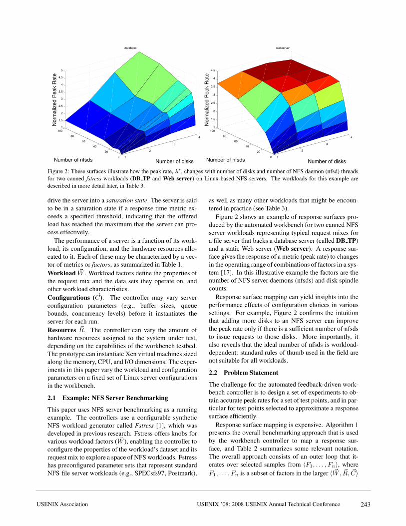
Figure 2: These surfaces illustrate how the peak rate, λ∗, changes with number of disks and number of NFS daemon (nfsd) threads

for two canned fstress workloads (DB TP and Web server) on Linux-based NFS servers. The workloads for this example are

described in more detail later, in Table 3.

drive the server into a saturation state. The server is said

to be in a saturation state if a response time metric ex-

ceeds a specified threshold, indicating that the offered

load has reached the maximum that the server can pro-

cess effectively.

The performance of a server is a function of its work-

load, its configuration, and the hardware resources allo-

cated to it. Each of these may be characterized by a vec-

tor of metrics or factors, as summarized in Table 1.

Workload ~W . Workload factors define the properties ofthe request mix and the data sets they operate on, and

other workload characteristics.

Configurations (~C). The controller may vary serverconfiguration parameters (e.g., buffer sizes, queue

bounds, concurrency levels) before it instantiates the

server for each run.

Resources ~R. The controller can vary the amount ofhardware resources assigned to the system under test,

depending on the capabilities of the workbench testbed.

The prototype can instantiate Xen virtual machines sized

along the memory, CPU, and I/O dimensions. The exper-

iments in this paper vary the workload and configuration

parameters on a fixed set of Linux server configurations

in the workbench.

2.1 Example: NFS Server Benchmarking

This paper uses NFS server benchmarking as a running

example. The controllers use a configurable synthetic

NFS workload generator called Fstress [1], which was

developed in previous research. Fstress offers knobs for

various workload factors ( ~W ), enabling the controller toconfigure the properties of the workload’s dataset and its

request mix to explore a space of NFSworkloads. Fstress

has preconfigured parameter sets that represent standard

NFS file server workloads (e.g., SPECsfs97, Postmark),

as well as many other workloads that might be encoun-

tered in practice (see Table 3).

Figure 2 shows an example of response surfaces pro-

duced by the automated workbench for two canned NFS

server workloads representing typical request mixes for

a file server that backs a database server (called DB TP)

and a static Web server (Web server). A response sur-

face gives the response of a metric (peak rate) to changes

in the operating range of combinations of factors in a sys-

tem [17]. In this illustrative example the factors are the

number of NFS server daemons (nfsds) and disk spindle

counts.

Response surface mapping can yield insights into the

performance effects of configuration choices in various

settings. For example, Figure 2 confirms the intuition

that adding more disks to an NFS server can improve

the peak rate only if there is a sufficient number of nfsds

to issue requests to those disks. More importantly, it

also reveals that the ideal number of nfsds is workload-

dependent: standard rules of thumb used in the field are

not suitable for all workloads.

2.2 Problem Statement

The challenge for the automated feedback-driven work-

bench controller is to design a set of experiments to ob-

tain accurate peak rates for a set of test points, and in par-

ticular for test points selected to approximate a response

surface efficiently.

Response surface mapping is expensive. Algorithm 1

presents the overall benchmarking approach that is used

by the workbench controller to map a response sur-

face, and Table 2 summarizes some relevant notation.

The overall approach consists of an outer loop that it-

erates over selected samples from 〈F1, . . . , Fn〉, whereF1, . . . , Fn is a subset of factors in the larger 〈 ~W, ~R, ~C〉


space (Step 2). The inner loop (Step 3) finds the peak rate

λ∗ for each sample by generating a series of test loads

for the sample. For each test load λ, the controller mustchoose the runlength r or observation interval, and thenumber of independent trials t to obtain a response timemeasure under load λ.

The goal of the automated feedback-driven controller

is to address the following problems.

1. Find Peak Rate (§3). For a given sample fromthe outer loop of Algorithm 1, minimize the bench-

marking cost for finding the peak rate λ∗ subject to

a target confidence level c and target accuracy a (de-fined below). Determining the NFSOPS rating of an

NFS filer is one instance of this problem.

2. Map Response Surface (§4). Minimize the totalbenchmarking cost to map a response surface for

all 〈F1, . . . , Fn〉 samples in the outer loop of Algo-rithm 1.

Minimizing benchmarking cost involves choosing val-

ues carefully for the runlength r, the number of trials t,and test loads λ so that the controller converges quicklyto the peak rate. Sections 3 and 4 present algorithms that

the controller uses to address these problems.

2.3 Confidence and Accuracy

Benchmarking can never produce an exact result because

complex systems exhibit inherent variability in their be-

havior. The best we can do is to make a probabilistic

claim about the interval in which the “true” value for a

metric lies based on measurements from multiple inde-

pendent trials [13]. Such a claim can be characterized

by a confidence level and the confidence interval at this

confidence level. For example, by observing the mean

response time R at a test load λ for 10 independent tri-als, we may be able to claim that we are 95% confident(the confidence level) that the correct value of R for thatλ lies within the range [25ms, 30ms] (the confidence in-terval).

Basic statistics tells us how to compute confidence in-

tervals and levels from a set of trials. For example, if the

mean server response time R from t trials is µ, and stan-dard deviation is σ, then the confidence interval for µ atconfidence level c is given by:

[µ − zcσ√t, µ +

zcσ√t] (1)

zc is a reading from the table of standard normal distri-

bution for confidence level c. If t <= 30, then we useStudent’s t distribution instead after verifying that the truns come from a normal distribution [13].

The tightness of the confidence interval captures the

accuracy of the true value of the metric. A tighter bound

λ∗ Peak rate for a given server configuration and

workload.

λ Offered load (arrival rate) for a given test load

level.

ρ Load factor= λ/λ∗ for a test load λ.R Mean server response time for a test load.

Rsat Threshold for R at the peak rate: the server issaturated if R > Rsat.

s Factor that determines the width of the peak-

rate region [Rsat ± sRsat] (§3.3).a Target accuracy (based on confidence interval

width) for the estimated value of λ∗ (§2.3).c Target confidence level for the estimated λ∗

(§2.3).t Number of independent trials at a test load.

r Runlength: the test interval over which to ob-

serve the server latency for each trial.

Table 2: Benchmarking parameters used in this paper.

implies that the mean response time from a set of tri-

als is closer to its true value. For a confidence interval

[low, high], we compute the percentage accuracy as:

accuracy = 1 − error = (1 − high− low

high + low) (2)

3 Finding the Peak Rate

In the inner loop of Algorithm 1, the automated con-

troller searches for the peak rate λ∗ for some workload

and configuration given by a selected sample of factor

values in 〈F1, . . . , Fn〉. To find the peak rate it subjectsthe server to a sequence of test loads λ = [λ1, . . . , λl].The sequence of test loads should converge on an esti-

mate of the peak rate λ∗ that meets the target accuracy

and confidence.

We emphasize that this step is itself a common bench-

marking task to determine a standard rating for a server

configuration in industry (e.g., SPECsfs [6]).

3.1 Strawman: Linear Search with Fixed r and t

Common practice for finding the peak rate is to script a

sequence of runs for a standard workload at a fixed linear

sequence of escalating load levels, with a preconfigured

runlength r and number of trials t for each load level.The algorithm is in essence a linear search for the peak

rate: it starts at a default load level and increments the

load level (e.g., arrival rate) by some fixed increment un-

til it drives the server into saturation. The last load level

λ before saturation is taken as the peak rate λ∗. We refer

to this algorithm as strawman.

Strawman is not efficient. If the increment is too small,

then it requires many iterations to reach the peak rate. Its

cost is also sensitive to the difference between the peak

rate and the initial load level: more powerful server con-

figurations take longer to benchmark. A larger increment


Algorithm 1: Mapping Response Surfaces

1) Inputs: (a) 〈F1, . . . , Fn〉, which is the subset offactors of interest from the full set of factors in

〈 ~W, ~R, ~C〉; (b) Different possible settings of eachfactor;

2) // Outer Loop: Map Response Surface.

foreach distinct sample 〈F1 =f1, . . . , Fn =fn〉do

3) // Inner Loop: Find Peak Rate for the Sample.

Design a sequence of test loads [λ1, . . . , λl] tosearch for the peak rate λ∗;

foreach test load λ ∈ [λ1, . . . , λl] doChoose number of trials t for load λ;

Choose runlength r for each trial;

Configure server and workload generator

for the sample; Run t independent trials oflength r each, with workload generated atload λ;

end

Set λ∗ = λ, where λ ∈ [λ1, . . . , λl] is thelargest load that does not take the server to the

saturation state;

end

can converge on the peak rate faster, but then the test may

overshoot the peak rate and compromise accuracy. In ad-

dition, strawman misses opportunities to reduce cost by

taking “rough” readings at low cost early in the search,

and to incur only as much cost as necessary to obtain a

statistically sound reading once the peak rate is found.

A simple workbench controller with feedback can im-

prove significantly on the strawman approach to search-

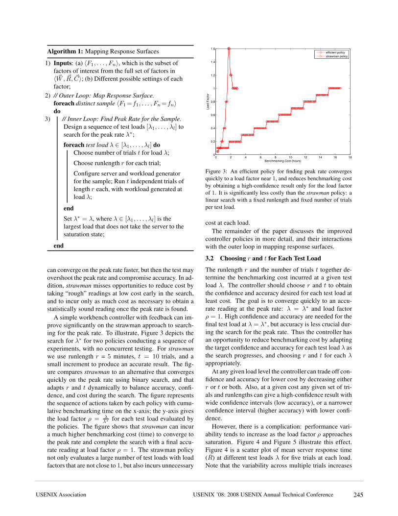
ing for the peak rate. To illustrate, Figure 3 depicts the

search for λ∗ for two policies conducting a sequence of

experiments, with no concurrent testing. For strawman

we use runlength r = 5 minutes, t = 10 trials, and asmall increment to produce an accurate result. The fig-

ure compares strawman to an alternative that converges

quickly on the peak rate using binary search, and that

adapts r and t dynamically to balance accuracy, confi-dence, and cost during the search. The figure represents

the sequence of actions taken by each policy with cumu-

lative benchmarking time on the x-axis; the y-axis gives

the load factor ρ = λλ∗for each test load evaluated by

the policies. The figure shows that strawman can incur

a much higher benchmarking cost (time) to converge to

the peak rate and complete the search with a final accu-

rate reading at load factor ρ = 1. The strawman policynot only evaluates a large number of test loads with load

factors that are not close to 1, but also incurs unnecessary

0 2 4 6 8 10 12 14 16 180

0.2

0.4

0.6

0.8

1

1.2

1.4

1.6

Lo

ad

Fa

cto

r

Benchmarking Cost (hours)

efficient policy

strawman policy

Figure 3: An efficient policy for finding peak rate converges

quickly to a load factor near 1, and reduces benchmarking cost

by obtaining a high-confidence result only for the load factor

of 1. It is significantly less costly than the strawman policy: a

linear search with a fixed runlength and fixed number of trials

per test load.

cost at each load.

The remainder of the paper discusses the improved

controller policies in more detail, and their interactions

with the outer loop in mapping response surfaces.

3.2 Choosing r and t for Each Test Load

The runlength r and the number of trials t together de-termine the benchmarking cost incurred at a given test

load λ. The controller should choose r and t to obtainthe confidence and accuracy desired for each test load at

least cost. The goal is to converge quickly to an accu-

rate reading at the peak rate: λ = λ∗ and load factor

ρ = 1. High confidence and accuracy are needed for thefinal test load at λ = λ∗, but accuracy is less crucial dur-

ing the search for the peak rate. Thus the controller has

an opportunity to reduce benchmarking cost by adapting

the target confidence and accuracy for each test load λ asthe search progresses, and choosing r and t for each λappropriately.

At any given load level the controller can trade off con-

fidence and accuracy for lower cost by decreasing either

r or t or both. Also, at a given cost any given set of tri-als and runlengths can give a high-confidence result with

wide confidence intervals (low accuracy), or a narrower

confidence interval (higher accuracy) with lower confi-

dence.

However, there is a complication: performance vari-

ability tends to increase as the load factor ρ approachessaturation. Figure 4 and Figure 5 illustrate this effect.

Figure 4 is a scatter plot of mean server response time

(R) at different test loads λ for five trials at each load.Note that the variability across multiple trials increases


0 0.2 0.4 0.6 0.8 1 1.2 1.4 1.60

10

20

30

40

50

60

70

80

90

Load Factor

Response

Tim

e(m

s)

Figure 4: Mean server response time at different test loads for

the DB TP fstress workload using 1 disk and 4 NFS daemon

(nfsd) threads for the server. The variability in mean server re-

sponse time for multiple trials increases with load. The results

are representative of other server configurations and workloads.

as λ → λ∗ and ρ → 1. Figure 5 shows a scatter plotof R measures for multiple runlengths at two load fac-tors, ρ = 0.3 and ρ = 0.9. Longer runlengths showless variability at any load factor, but for a given run-

length, the variability is higher at the higher load factor.

Thus the cost for any level of confidence and/or accuracy

also depends on load level: since variability increases at

higher load factors, it requires longer runlengths r and/ora larger number of trials t to reach a target level of confi-dence and accuracy.

For example, consider the set of trials plotted in Fig-

ure 5. At load factor 0.3 and runlength of 90 seconds,the data gives us 70% confidence that 5.6 < R < 6, or95% confidence that 5 < R < 6.5. From the data we candetermine the runlength needed to achieve target confi-

dence and accuracy at this load level and number of tri-

als t: a runlength of 90 seconds achieves an accuracy of87%with 95% confidence, but it takes a runlength of 300seconds to achieve 95% accuracy with 95% confidence.Accuracy and confidence decrease with higher load fac-

tors. For example, at load factor 0.9 and runlength 90, thedata gives us 70% confidence that 21 < R < 24 (93.3%accuracy), or 95% confidence that 20 < R < 27 (85.1%accuracy). As a result, we must increase the runlength

and/or the number of trials to maintain target levels of

confidence and accuracy as load factors increase. For

example, we need a runlength of 120 seconds or moreto achieve accuracy ≥ 87% at 95% confidence for thisnumber of trials at load factor 0.9.

Figure 6 quantifies the tradeoff between the runlength

and the number of trials required to attain a target ac-

curacy and confidence for different workloads and load

factors. It shows the number of trials required to meet

Algorithm 2: Searching for the Peak Rate

1) Initialization. Peak Rate, λ∗ = 0; Currentaccuracy of the peak rate, aλ∗ = 0; Current testload, λcur = 0; Previous test load, λprev = 0;

2) Use Algorithm 3 to choose a test load λ by givingcurrent test load λcur, previous test load λprev , and

mean server response time Rλcurat λcur as inputs;

3) Set λprev = λcur and λcur = λ;

4) while (aλ∗ < a at confidence c)

5) Choose the runlength r for the trial;

6) Conduct the trial at λcur, and measure server

response time from this trial, Rλcur;

7) Compute mean server response time at

λcur, Rλcur, from all trials at λcur. Repeat Step 6

if the number of trials, t, at λcur is 1;

8) Compute confidence interval for the mean

server response Rλcurat target confidence level c;

9) Check for overlap between the confidence

interval for Rλcurand the peak rate region;

10) if (no overlap with 95% confidence)

Go to Step 2 to choose the next test load;

else

λ∗ = λcur;

Compute accuracy aλ∗ at confidence c;

end

end

an accuracy of 90% at 95% confidence level for differ-ent runlengths. The figure shows that to attain a target

accuracy and confidence, one needs to conduct more in-

dependent trials at shorter runlengths. It also shows a

sweet spot for the runlengths that reduces the number of

trials needed. A controller can use such curves as a guide

to pick a suitable runlength r and number of trials t withlow cost.

3.3 Search Algorithm

Our approach uses Algorithm 2 to search for the peak

rate for a given setting of factors.

Algorithm 2 takes various parameters to define the

conditions for the reported peak rate:

• Rsat, a threshold on the mean server response time.

The server is considered to be saturated if mean re-

sponse time exceeds this threshold, i.e., R > Rsat.

• Psat and Lsat defining a threshold on percentile

server response time. The server is considered to

be saturated if the Psat percentile response time ex-

ceeds Lsat. For example, if Psat = 0.95 then the


0 50 100 150 200 250 3000

4

5

6

7

8

9

10

11

12

Runlength (secs)

Response

Tim

e(m

s)

load factor (ρ) = 0.3

0 50 100 150 200 250 3000

10

20

30

40

50

60

Runlength (secs)

Response

Tim

e(m

s)


Figure 5: Mean server response time R at different workload runlengths for the DB TP fstress workload using 1 disk and 4 NFS

daemon (nfsd) threads for the server. The variability in mean server response time for multiple trials decreases with increase in

runlength. The results are representative of other server configurations and workloads.

server is saturated if no more than 95% of responses

show latency at or below Lsat. To simplify the pre-

sentation we use the Rsat threshold test on mean

response time and do not discuss Psat further.

• Width parameter s defining the peak-rate region[Rsat ± sRsat]. The reported peak rate λ∗ can be

any test load level that drives the mean server re-

sponse time into this region. (The region [Psat ±sPsat] is defined similarly.)

• Target confidence c in the peak rate that the algo-rithm estimates.

• Target accuracy a of the peak rate that the algorithmestimates.

Algorithm 2 chooses (a) a sequence of test loads to try;

(b) the number of independent trials at any test load; and

(c) the runlength of the workload at that load. It automat-

ically adapts the number of trials at any test load accord-

ing to the load factor and the desired target confidence

and accuracy. At each load level the algorithm conducts

a small (often the minimum of two in our experiments)

number of trials to establish with 95% confidence thatthe current test load is not the peak rate (Step 10). How-ever, as soon as the algorithm identifies a test load λ tobe a potential peak rate, which happens near a load factor

of 1, it spends just enough time to check whether it is infact the peak rate.

More specifically, for each test load λcur, Algorithm 2

first conducts two trials to generate an initial confidence

interval for Rλcur, the mean server response time at load

λcur, at 95% confidence level. (Steps 6 and 7 in Algo-rithm 2.) Next, it checks if the confidence interval over-

laps with the specified peak-rate region (Step 9).

If the regions overlap, then Algorithm 2 identifies the

current test load λcur as an estimate of a potential peak

rate with 95% confidence. It then computes the accuracy

of the mean server response time Rλcurat the current test

load, at the target confidence level c (Section 2.1). If itreaches the target accuracy a, then the algorithm termi-nates (Step 4), otherwise it conducts more trials at thecurrent test load (Step 6) to narrow the confidence inter-val, and repeats the threshold condition test. Thus the

cost of the algorithm varies with the target confidence

and accuracy.

If there is no overlap (Step 10), then Algorithm 2moves on to the next test load. It uses any of several load-

picking algorithms to generate the sequence of test loads,

described in the rest of this section. All load-picking al-

gorithms take as input the set of past test loads and their

results. The output becomes the next test load in Algo-

rithm 2. For example, Algorithm 3 gives a load-picking

algorithm using a simple binary search.

To simplify the choice of runlength for each experi-

ment at a test load (Step 5), Algorithm 2 uses the “sweet

spot” derived from Figure 6 (Section 3.2). The figure

shows that for all workloads that this paper considers, a

runlength of 3minutes is the sweet spot for the minimumnumber of trials.

3.4 The Binsearch Load-Picking Algorithm

Algorithm 3 outlines the Binsearch algorithm. Intu-

itively, Binsearch keeps doubling the current test load un-

til it finds a load that saturates the server. After that, Bin-

search applies regular binary search, i.e., it recursively

halves the most recent interval of test loads where the

algorithm estimates the peak rate to lie.

Binsearch allows the controller to find the lower and


0 50 100 150 200 250 300 3500

50

100

150

Runlength (secs)

Nu

mb

er

of

tria

ls


DB_TP

Webserver

Mail

Specsfs97

0 50 100 150 200 250 300 3500

50

100

150

Runlength (secs)

Nu

mb

er

of

tria

ls


DB_TP

Webserver

Mail

Specsfs97

Figure 6: Number of trials to attain 90% accuracy for mean server response time at 95% confidence level at low and high load

factors for different runlengths. The results are for server configuration with 1 disk and 4 nfsds, and representative of other server

configurations.

Algorithm 3: Binsearch Input: Previous load λprev;

Current load λcur ; Mean response time Rλcurat λcur;

Output: Next load λnext

1) Initialization.

if (λcur == 0);λnext = 50 requests/sec;Phase = Geometric; Return λnext;

2) Geometric Phase.

if (Phase == Geometric && Rλcur< Rsat)

Return λnext = λcur × 2;elsebinsearchlow = λprev , and Go to Step 3;

end

3) Binary Search Phase.

if ( Rλcur< Rsat) ;

binsearchlow = λcur;

else

binsearchhigh = λcur;

end

Return λnext = (binsearchhigh + binsearchlow)/2;

upper bounds for the peak rate within a logarithmic num-

ber of test loads. The controller can then estimate the

peak rate using another logarithmic number of test loads.

Hence the total number of test loads is always logarith-

mic irrespective of the start test load or the peak rate.

3.5 The Linear Load-Picking Algorithm

The Linear algorithm is similar to Binsearch except in

the initial phase of finding the lower and upper bounds

for the peak rate. In the initial phase it picks an increas-

ing sequence of test loads such that each load differs

from the previous one by a small fixed increment.

3.6 Model-guided Load-Picking Algorithm

The general shape of the response-time vs. load curve

is well known, and the form is similar for different

workloads and server configurations. This suggests that

a model-guided approach could fit the curve from a

few test loads and converge more quickly to the peak

rate. Using the insight offered by well-known open-loop

queuing theory results [13], we experimentedwith a sim-

ple model to fit the curve: R = 1/(a− b∗λ), whereR isthe response time, λ is the load, and a and b are constantsthat depend on the settings of factors in 〈 ~W, ~R, ~C〉. Tolearn the model, the controller needs tuples of the form

〈λ, Rλ〉.Algorithm 4 outlines the model-guided algorithm. If

there are insufficient tuples for learning the model, it uses

a simple heuristic to pick the test loads for generating the

tuples. After that, the algorithm uses the model to predict

the peak rate λ = λ∗ for R = Rsat, returns the predic-

tion as the next test load, and relearns the model using the

new 〈λ, Rλ〉 tuple at the prediction. The whole processrepeats until the search converges to the peak rate. As

the controller observes more 〈λ, Rλ〉 tuples, the model-fit should improve progressively, and the model should

guide the search to an accurate peak rate. In many cases,

this happens in a single iteration of model learning (Sec-

tion 5).

However, unlike the previous approaches, a model-

guided search is not guaranteed to converge. Model-

guided search is dependent on the accuracy of the model,

which in turn depends on the choice of 〈λ, Rλ〉 tuplesthat are used for learning. The choice of tuples is gen-


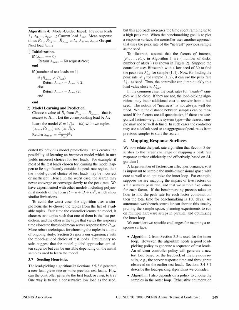
Algorithm 4: Model-Guided Input: Previous loads

λ1, λ2, ..., λcur−1; Current load λcur; Mean response

times Rλ1, Rλ2

, ..., Rλcurat λ1, λ2, ..., λcur; Output:

Next load λnext

1) Initialization.

if (λcur == 0)Return λnext = 50 requests/sec;

end

if (number of test loads == 1)

if (Rλcur< Rsat)

Return λnext = λcur × 2;else

Return λnext = λcur/2;end

end

2) Model Learning and Prediction.

Choose a value of Ri from Rλ1, ..., Rλcur−1

that is

nearest to Rsat. Let the corresponding load be λi;

Learn the modelR = 1/(a − bλ) with two tuples〈λcur, Rλcur

〉 and 〈λi, Ri〉;Return λnext = Rsata−1

Rsatb;

erated by previous model predictions. This creates the

possibility of learning an incorrect model which in turn

yields incorrect choices for test loads. For example, if

most of the test loads chosen for learning the model hap-

pen to lie significantly outside the peak rate region, then

the model-guided choice of test loads may be incorrect

or inefficient. Hence, in the worst case, the search may

never converge or converge slowly to the peak rate. We

have experimented with other models including polyno-

mial models of the formR = a + bλ + cλ2, which show

similar limitations.

To avoid the worst case, the algorithm uses a sim-

ple heuristic to choose the tuples from the list of avail-

able tuples. Each time the controller learns the model, it

chooses two tuples such that one of them is the last pre-

diction, and the other is the tuple that yields the response

time closest to thresholdmean server response timeRsat.

More robust techniques for choosing the tuples is a topic

of ongoing study. Section 5 reports our experience with

the model-guided choice of test loads. Preliminary re-

sults suggest that the model-guided approaches are of-

ten superior but can be unstable depending on the initial

samples used to learn the model.

3.7 Seeding Heuristics

The load-picking algorithms in Sections 3.5-3.6 generate

a new load given one or more previous test loads. How

can the controller generate the first load, or seed, to try?

One way is to use a conservative low load as the seed,

but this approach increases the time spent ramping up to

a high peak rate. When the benchmarking goal is to plot

a response surface, the controller uses another approach

that uses the peak rate of the “nearest” previous sample

as the seed.

To illustrate, assume that the factors of interest,

〈F1, . . . , Fn〉, in Algorithm 1 are 〈 number of disks,number of nfsds 〉 (as shown in Figure 2). Suppose thecontroller uses Binsearch with a low seed of 50 to findthe peak rate λ∗

1,1 for sample 〈1, 1〉. Now, for finding thepeak rate λ∗

1,2 for sample 〈1, 2〉, it can use the peak rateλ∗

1,1 as seed. Thus, the controller can jump quickly to a

load value close to λ∗1,2.

In the common case, the peak rates for “nearby” sam-

ples will be close. If they are not, the load-picking algo-

rithms may incur additional cost to recover from a bad

seed. The notion of “nearness” is not always well de-

fined. While the distance between samples can be mea-

sured if the factors are all quantitative, if there are cate-

gorical factors—e.g., file system type—the nearest sam-

ple may not be well defined. In such cases the controller

may use a default seed or an aggregate of peak rates from

previous samples to start the search.

4 Mapping Response Surfaces

We now relate the peak rate algorithm that Section 3 de-

scribes to the larger challenge of mapping a peak rate

response surface efficiently and effectively, based on Al-

gorithm 1.

A large number of factors can affect performance, so it

is important to sample the multi-dimensional space with

care as well as to optimize the inner loop. For example,

suppose we are mapping the impact of five factors on

a file server’s peak rate, and that we sample five values

for each factor. If the benchmarking process takes an

hour to find the peak rate for each factor combination,

then the total time for benchmarking is 130 days. Anautomated workbench controller can shorten this time by

pruning the sample space, planning experiments to run

on multiple hardware setups in parallel, and optimizing

the inner loop.

We consider two specific challenges for mapping a re-

sponse surface:

• Algorithm 2 from Section 3.3 is used for the innerloop. However, the algorithm needs a good load-

picking policy to generate a sequence of test loads.

An efficient controller policy will generate a new

test load based on the feedback of the previous re-

sults, e.g., the server response time and throughput

observed on the earlier test loads. Sections 3.4-3.7

describe the load-picking algorithms we consider.

• Algorithm 1 also depends on a policy to choose thesamples in the outer loop. Exhaustive enumeration


of the full factor space in the outer loop can incur

an exorbitant benchmarking cost. Depending on the

goal of the benchmarking exercise, the controller

can choose more efficient techniques.

If the benchmarking objective is to understand the

overall trend of how the peak rate is affected by

certain factors of interest 〈F1, . . . , Fn〉—rather thanfinding accurate peak rate values for each sample in

〈F1, . . . , Fn〉—then Algorithm 1 can leverage ResponseSurface Methodology (RSM) [17] to select the sample

points efficiently (in Step 2). RSM is a branch of statis-

tics that provides principled techniques to choose a set

of samples to obtain good approximations of the overall

response surface at low cost. For example, some RSM

techniques assume that a low-degree multivariate poly-

nomial model— e.g., a quadratic equation of the form

λ∗ = β0 +∑n

i=1βiFi +

∑n

i=1

∑n

j=1,j 6=i βijFiFj +∑n

i=1βiiFi

2— approximates the surface in the n-dimensional 〈F1, . . . , Fn〉 space. This approximation isa basis for selecting a minimal set of samples for the con-

troller to obtain in order to learn a fairly accurate model

(i.e., estimate values of the β parameters in the model).We evaluate one such RSM technique in Section 5.

It is important to note that these RSM techniques may

reduce the effectiveness of the seeding heuristics de-

scribed in Section 3.7. RSM techniques try to find sam-

ple points on the surface that will add the most informa-

tion to the model. Intuitively, such samples are the ones

that we have the least prior information about, and hence

for which seeding from prior results would be least ef-

fective. We leave it to future work to explore the inter-

actions of the heuristics for selecting samples efficiently

and seeding the peak rate search for each sample.

5 Experimental Evaluation

We evaluate the benchmarkingmethodology and policies

with multiple workloads on the following metrics.

Cost for Finding Peak Rate. Sections 3.3 and 4 present

several policies for finding the peak rate. We evaluate

those policies as follows:

• The sequence of load factors that the policies con-sider before converging to the peak rate for a sam-

ple. An efficient policy must quickly direct the

search to load factors that are near or at 1.

• The number of independent trials for each load fac-tor. The number of trials should be less at low load

factors and high around load factor of 1.

Cost forMapping Response Surfaces. We compare the

total benchmarking cost for mapping the response sur-

face across all the samples.

Cost Versus Target Confidence and Accuracy. We

demonstrate that the policies adapt the total benchmark-

ing cost to target confidence and accuracy. Higher confi-

dence and accuracy incurs higher benchmarking cost and

vice-versa.

Section 5.1 presents the experiment setup. Section 5.2

presents the workloads that we use for evaluation. Sec-

tion 5.3 evaluates our benchmarking methodology as de-

scribed above.

5.1 Experimental Setup

Table 1 shows the factors in the 〈 ~W, ~R, ~C〉 vectors fora storage server. We benchmark an NFS server to eval-

uate our methodology. In our evaluation, the factors in~W consist of samples that yield four types of workloads:SPECsfs97, Web server, Mail server, and DB TP (Sec-

tion 5.2). The controller uses Fstress to generate sam-

ples of ~W that correspond to these workloads. We reportresults for a single factor in ~R: the number of disks at-tached to the NFS server in 〈1, 2, 3, 4〉, and a single fac-tor in ~C: the number of nfsd daemons for the NFS serverchosen from 〈1, 2, 4, 8, 16, 32, 64, 100〉 to give us a totalof 32 samples.The workbench tools can generate both virtual and

physical machine configurations automatically. In our

evaluation we use physical machines that have 800 MBmemory, 2.4 GHz x86 CPU, and run the 2.6.18 Linuxkernel. To conduct an experiment, the workbench con-

troller first prepares an experiment by generating a sam-

ple in 〈 ~W , ~R, ~C〉. It then consults the benchmarkingpolicy(ies) in Sections 3.4-4 to plot a response surface

and/or search for the peak rate for a given sample with

target confidence and accuracy.

5.2 Workloads

We use Fstress to generate ~W corresponding to four

workloads as summarized in Table 3. A brief summary

follows. Further details are in [1].

• SPECsfs97: The Standard Performance EvaluationCorporation introduced their System File Server

benchmark (SPECsfs) [6] in 1992, derived from the

earlier self-scaling LADDIS benchmark [15]. A re-

cent (2001) revision corrected several defects iden-

tified in the earlier version [11].

• Web server: Several efforts (e.g., [2]) attempt toidentify durable characterizations of the Web. We

derive the distributions for various parameters and

the operation mix from the previous published stud-

ies (e.g., [19, 8, 18, 9, 2]).

• DB TP: We model our database workload afterTPC-C [7], reading and writing within a few large

files in a 2:1 ratio. I/O access patterns are ran-

dom, with some short (256 KB) sequential asyn-


workload file popularities file sizes dir sizes I/O accesses

SPECsfs97 random 10% 1 KB – 1 MB large (thousands) random r/w

Web server Zipf (0.6 < α < 0.9) long-tail (avg 10.5 KB) small (dozens) sequential reads

DB TP few files large (GB - TB) small random r/w

Mail Zipf (α = 1.3) long-tail (avg 4.7 KB) large (500+) seq r, append w

Table 3: Summary of fstress workloads used in the experiments.

chronouswrites with commit (fsync) to mimic batch

log writes.

• Mail: Electronic mail servers frequently handlemany small files, one file per users’ mailbox.

Servers append incoming messages, and sequen-

tially read the mailbox file for retrieval. Some users

or servers truncate mailboxes after reading. The

workload model follows that proposed by Saito et

al. [20].

5.3 Results

For evaluating the overall methodology and the policies

outlined in Sections 3.3 and 4, we define the peak rate

λ∗ to be the test load that causes: (a) the mean server

response time to be in the [36, 44] ms region; or (b) the95-percentile request response time to exceed 2000 msto complete. We derive the [36, 44] region by choosingmean server response time threshold at the peak rateRsat

to be 40ms and the width factor s = 10% in Table 2. Forall results except where we note explicitly, we aim for a

λ∗ to be accurate within 10% of its true value with 95%confidence.

5.3.1 Cost for Finding Peak Rate

Figure 7 shows the choice of load factors for finding the

peak rate for a sample with 4 disks and 32 nfsds usingthe policies outlined in Section 4. Each point on the

curve represents a single trial for some load factor. More

points indicate higher number of trials at that load factor.

For brevity, we show the results only for DB TP. Other

workloads show similar behavior.

For all policies, the controller conducts more trials at

load factors near 1 than at other load factors to find thepeak rate with the target accuracy and confidence. All

policies without seeding start at a low load factor and

take longer to reach a load factor of 1 as compared topolicies with seeding. All policies with seeding start at

a load factor close to 1, since they use the peak rate ofa previous sample with 4 disks and 16 nfsds as the seedload.

Linear takes a significantly longer time because it uses

a fixed increment by which to increase the test load.

However, Binsearch jumps to the peak rate region in log-

arithmic number of steps. TheModel policy is the quick-

est to jump near the load factor of 1, but incurs most ofits cost there. This happens because the model learned

is sufficiently accurate for guiding the search near the

peak rate, but not accurate enough to search the peak rate

quickly.

0 1 2 3 4 5 60

0.5

1

1.5

2

Load

Facto

r

Time (hours)

linear

linear.seeding

0 1 2 3 4 5 60

0.5

1

1.5

2

Load

Facto

r

Time (hours)

binsearch

binsearch.seeding

0 1 2 3 4 5 60

0.5

1

1.5

2Load

Facto

r

Time (hours)

model

model.seeding

Figure 7: Time spent at each load factor for finding the peak

rate for different policies forDB TP with 4 disks and 32 nfsds.

Seeded policies were seeded with the peak rate for 4 disks and

16 nfsds. The result is representative of other samples and

workloads. All policies except linear quickly converge to the

load factor of 1 and conduct more trials there to achieve the

target accuracy and confidence.

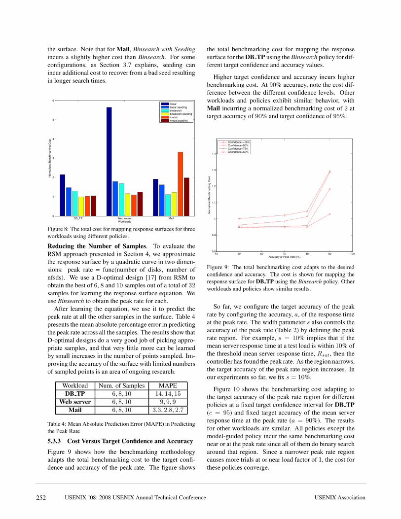
5.3.2 Cost for Mapping Response Surfaces

Figure 8 compares the total normalized benchmarking

cost for mapping the response surfaces for the three

workloads using the policies outlined in Section 4. The

costs are normalized with respect to the lowest total cost,

which is 47 hours and 36 minutes taken by the Binsearch

with Seeding policy to find the peak rate forDB TP. Bin-

search, Binsearch with Seeding, and Linear with Seeding

cut the total cost drastically as compared to the linear

policy.

We also observe that Binsearch, Binsearch with Seed-

ing, and Linear with Seeding are robust across the work-

loads, but the model-guided policy is unstable. This

is not surprising given that the accuracy of the learned

model guides the search. As Section 3.6 explains, if the

model is inaccurate the search may converge slowly.

The linear policy is inefficient and highly sensitive to

the magnitude of peak rate. The benchmarking cost of

Linear forWeb server peaks at a higher absolute value

for all samples than for DB TP andMail, causing more

than a factor of 5 increase in the total cost for mapping


the surface. Note that forMail, Binsearch with Seeding

incurs a slightly higher cost than Binsearch. For some

configurations, as Section 3.7 explains, seeding can

incur additional cost to recover from a bad seed resulting

in longer search times.

DB_TP Web server Mail0

1

2

3

4

5

6

Workloads

Norm

aliz

ed

Benchm

ark

ing

Cost

linear

linear.seeding

binsearch

binsearch.seeding

model

model.seeding

Figure 8: The total cost for mapping response surfaces for three

workloads using different policies.

Reducing the Number of Samples. To evaluate the

RSM approach presented in Section 4, we approximate

the response surface by a quadratic curve in two dimen-

sions: peak rate = func(number of disks, number of

nfsds). We use a D-optimal design [17] from RSM to

obtain the best of 6, 8 and 10 samples out of a total of 32samples for learning the response surface equation. We

use Binsearch to obtain the peak rate for each.

After learning the equation, we use it to predict the

peak rate at all the other samples in the surface. Table 4

presents the mean absolute percentage error in predicting

the peak rate across all the samples. The results show that

D-optimal designs do a very good job of picking appro-

priate samples, and that very little more can be learned

by small increases in the number of points sampled. Im-

proving the accuracy of the surface with limited numbers

of sampled points is an area of ongoing research.

Workload Num. of Samples MAPE

DB TP 6, 8, 10 14, 14, 15Web server 6, 8, 10 9, 9, 9Mail 6, 8, 10 3.3, 2.8, 2.7

Table 4: Mean Absolute Prediction Error (MAPE) in Predicting

the Peak Rate

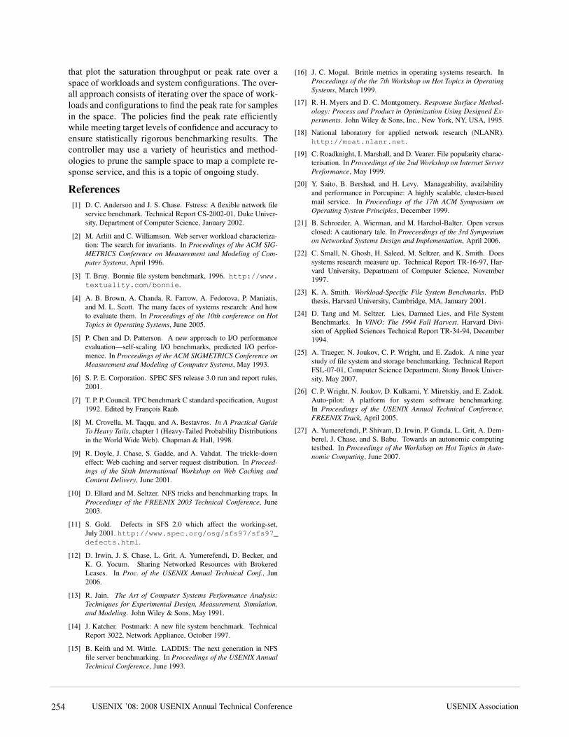
5.3.3 Cost Versus Target Confidence and Accuracy

Figure 9 shows how the benchmarking methodology

adapts the total benchmarking cost to the target confi-

dence and accuracy of the peak rate. The figure shows

the total benchmarking cost for mapping the response

surface for theDB TP using the Binsearch policy for dif-

ferent target confidence and accuracy values.

Higher target confidence and accuracy incurs higher

benchmarking cost. At 90% accuracy, note the cost dif-ference between the different confidence levels. Other

workloads and policies exhibit similar behavior, with

Mail incurring a normalized benchmarking cost of 2 attarget accuracy of 90% and target confidence of 95%.

40 50 60 70 80 90 1000.8

0.9

1

1.1

1.2

1.3

1.4

Norm

aliz

ed

Benchm

ark

ing

Cost

Accuracy of Peak Rate (%)

Confidence = 95%

Confidence=90%

Confidence=75%

Confidence=60%

Figure 9: The total benchmarking cost adapts to the desired

confidence and accuracy. The cost is shown for mapping the

response surface for DB TP using the Binsearch policy. Other

workloads and policies show similar results.

So far, we configure the target accuracy of the peak

rate by configuring the accuracy, a, of the response timeat the peak rate. The width parameter s also controls theaccuracy of the peak rate (Table 2) by defining the peak

rate region. For example, s = 10% implies that if themean server response time at a test load is within 10% ofthe threshold mean server response time, Rsat, then the

controller has found the peak rate. As the region narrows,

the target accuracy of the peak rate region increases. In

our experiments so far, we fix s = 10%.

Figure 10 shows the benchmarking cost adapting to

the target accuracy of the peak rate region for different

policies at a fixed target confidence interval for DB TP

(c = 95) and fixed target accuracy of the mean serverresponse time at the peak rate (a = 90%). The resultsfor other workloads are similar. All policies except the

model-guided policy incur the same benchmarking cost

near or at the peak rate since all of them do binary search

around that region. Since a narrower peak rate region

causes more trials at or near load factor of 1, the cost forthese policies converge.


0

0.5

1

1.5

2

2.5

3

3.5

4

90 92 94 96 98 100

No

rma

lize

dB

en

ch

ma

rkin

gC

ost

Accuracy of Peak Rate (%)

linearlinear.seeding

binsearchbinsearch.seeding

modelmodel.seeding

Figure 10: Benchmarking cost adapts to the target accuracy of

the peak rate region for all policies. As the region narrows, the

majority of the cost is incurred at or near the peak rate. Linear

and Binsearch incur the same cost close to the peak rate, and

hence their cost converges as they conduct more trials near the

peak rate. The cost is shown forDB TP. Other workloads show

similar results.

6 Related Work

Several researchers have made a case for statistically

significant results from system benchmarking, e.g., [4].

Auto-pilot [26] is a system for automating the bench-

marking process: it supports various benchmark-related

tasks and can modulate individual experiments to obtain

a target confidence and accuracy. Our goal is to take

the next step and focus on an automation framework and

policies to orchestrate sets of experiments for a higher

level benchmarking objective, such as evaluating a re-

sponse surface or obtaining saturation throughputs under

various conditions. We take the workbench test harness

itself as given, and our approach is compatible with ad-

vanced test harnesses such as Auto-pilot.

While there are large numbers and types of bench-

marks, (e.g., [5, 14, 3, 15]) that test the performance of

servers in a variety of ways, there is a lack of a general

benchmarking methodology that provides benchmark-

ing results from these benchmarks efficiently with con-

fidence and accuracy. Our methodology and techniques

for balancing the benchmarking cost and accuracy are

applicable to all these benchmarks.

Zadok et al. [25] present an exhaustive nine-year study

of file system and storage benchmarking that includes

benchmark comparisons, their pros and cons [22], and

makes recommendations for systematic benchmarking

methodology that considers a range of workloads for

benchmarking the server. Smith et al. [23] make a case

for benchmarks the capture composable elements of re-

alistic application behavior. Ellard et al. [10] show that

benchmarking an NFS server is challenging because of

the interactions between the server software configu-

rations, workloads, and the resources allocated to the

server. One of the challenges in understanding the inter-

actions is the large space of factors that govern such in-

teractions. Our benchmarking methodology benchmarks

a server across the multi-dimensional space of workload,

resource, and configuration factors efficiently and accu-

rately, and avoids brittle “claims” [16] and “lies” [24]

about a server performance.

Synthetic workloads emulate characteristics observed

in real environments. They are often self-scaling [5],

augmenting their capacity requirements with increasing

load levels. The synthetic nature of these workloads

enables them to preserve workload features as the file

set size grows. In particular, the SPECsfs97 bench-

mark [6] (and its predecessor LADDIS [15]) creates a

set of files and applies a pre-defined mix of NFS oper-

ations. The experiments in this paper use Fstress [1], a

synthetic, flexible, self-scaling NFS workload generator

that can emulate a range of NFS workloads, including

SPECsfs97. Like SPECsfs97, Fstress uses probabilistic

distributions to govern workload mix and access charac-

teristics. Fstress adds file popularities, directory tree size

and shape, and other controls. Fstress includes several

important workload configurations, such as Web server

file accesses, to simplify file system performance eval-

uation under different workloads [23] while at the same

time allowing standardized comparisons across studies.

Server benchmarking isolates the performance effects

of choices in server design and configuration, since it

subjects the server to a steady offered load independent

of its response time. Relative to other methodologies

such as application benchmarking, it reliably stresses the

system under test to its saturation point where interesting

performance behaviors may appear. In the storage arena,

NFS server benchmarking is a powerful tool for inves-

tigation at all layers of the storage stack. A workload

mix can be selected to stress any part of the system, e.g.,

the buffering/caching system, file system, or disk system.

By varying the components alone or in combination, it is

possible to focus on a particular component in the stor-

age stack, or to explore the interaction of choices across

the components.

7 Conclusion

This paper focuses on the problem of workbench au-

tomation for server benchmarking. We propose an auto-

mated benchmarking system that plans, configures, and

executes benchmarking experiments on a common hard-

ware pool. The activity is coordinated by an automated

controller that can consider various factors in planning,

sequencing, and conducting experiments. These factors

include accuracy vs. cost tradeoffs, availability of hard-

ware resources, deadlines, and the results reaped from

previous experiments.

We present efficient and effective controller policies


that plot the saturation throughput or peak rate over a

space of workloads and system configurations. The over-

all approach consists of iterating over the space of work-

loads and configurations to find the peak rate for samples

in the space. The policies find the peak rate efficiently

while meeting target levels of confidence and accuracy to

ensure statistically rigorous benchmarking results. The

controller may use a variety of heuristics and method-

ologies to prune the sample space to map a complete re-

sponse service, and this is a topic of ongoing study.

References

[1] D. C. Anderson and J. S. Chase. Fstress: A flexible network file

service benchmark. Technical Report CS-2002-01, Duke Univer-

sity, Department of Computer Science, January 2002.

[2] M. Arlitt and C. Williamson. Web server workload characteriza-

tion: The search for invariants. In Proceedings of the ACM SIG-

METRICS Conference on Measurement and Modeling of Com-

puter Systems, April 1996.

[3] T. Bray. Bonnie file system benchmark, 1996. http://www.

textuality.com/bonnie.

[4] A. B. Brown, A. Chanda, R. Farrow, A. Fedorova, P. Maniatis,

and M. L. Scott. The many faces of systems research: And how

to evaluate them. In Proceedings of the 10th conference on Hot

Topics in Operating Systems, June 2005.

[5] P. Chen and D. Patterson. A new approach to I/O performance

evaluation—self-scaling I/O benchmarks, predicted I/O perfor-

mence. In Proceedings of the ACM SIGMETRICS Conference on

Measurement and Modeling of Computer Systems, May 1993.

[6] S. P. E. Corporation. SPEC SFS release 3.0 run and report rules,

2001.

[7] T. P. P. Council. TPC benchmark C standard specification, August

1992. Edited by Francois Raab.

[8] M. Crovella, M. Taqqu, and A. Bestavros. In A Practical Guide

To Heavy Tails, chapter 1 (Heavy-Tailed Probability Distributions

in the World Wide Web). Chapman & Hall, 1998.

[9] R. Doyle, J. Chase, S. Gadde, and A. Vahdat. The trickle-down

effect: Web caching and server request distribution. In Proceed-

ings of the Sixth International Workshop on Web Caching and

Content Delivery, June 2001.

[10] D. Ellard and M. Seltzer. NFS tricks and benchmarking traps. In

Proceedings of the FREENIX 2003 Technical Conference, June

2003.

[11] S. Gold. Defects in SFS 2.0 which affect the working-set,

July 2001. http://www.spec.org/osg/sfs97/sfs97_

defects.html.

[12] D. Irwin, J. S. Chase, L. Grit, A. Yumerefendi, D. Becker, and

K. G. Yocum. Sharing Networked Resources with Brokered

Leases. In Proc. of the USENIX Annual Technical Conf., Jun

2006.

[13] R. Jain. The Art of Computer Systems Performance Analysis:

Techniques for Experimental Design, Measurement, Simulation,

and Modeling. John Wiley & Sons, May 1991.

[14] J. Katcher. Postmark: A new file system benchmark. Technical

Report 3022, Network Appliance, October 1997.

[15] B. Keith and M. Wittle. LADDIS: The next generation in NFS

file server benchmarking. In Proceedings of the USENIX Annual

Technical Conference, June 1993.

[16] J. C. Mogul. Brittle metrics in operating systems research. In

Proceedings of the the 7th Workshop on Hot Topics in Operating

Systems, March 1999.

[17] R. H. Myers and D. C. Montgomery. Response Surface Method-

ology: Process and Product in Optimization Using Designed Ex-

periments. John Wiley & Sons, Inc., New York, NY, USA, 1995.

[18] National laboratory for applied network research (NLANR).

http://moat.nlanr.net.

[19] C. Roadknight, I. Marshall, and D. Vearer. File popularity charac-

terisation. In Proceedings of the 2nd Workshop on Internet Server

Performance, May 1999.

[20] Y. Saito, B. Bershad, and H. Levy. Manageability, availability

and performance in Porcupine: A highly scalable, cluster-based

mail service. In Proceedings of the 17th ACM Symposium on

Operating System Principles, December 1999.

[21] B. Schroeder, A. Wierman, and M. Harchol-Balter. Open versus

closed: A cautionary tale. In Proeceedings of the 3rd Symposium

on Networked Systems Design and Implementation, April 2006.

[22] C. Small, N. Ghosh, H. Saleed, M. Seltzer, and K. Smith. Does

systems research measure up. Technical Report TR-16-97, Har-

vard University, Department of Computer Science, November

1997.

[23] K. A. Smith. Workload-Specific File System Benchmarks. PhD

thesis, Harvard University, Cambridge, MA, January 2001.

[24] D. Tang and M. Seltzer. Lies, Damned Lies, and File System

Benchmarks. In VINO: The 1994 Fall Harvest. Harvard Divi-

sion of Applied Sciences Technical Report TR-34-94, December

1994.

[25] A. Traeger, N. Joukov, C. P. Wright, and E. Zadok. A nine year

study of file system and storage benchmarking. Technical Report

FSL-07-01, Computer Science Department, Stony Brook Univer-

sity, May 2007.

[26] C. P. Wright, N. Joukov, D. Kulkarni, Y. Miretskiy, and E. Zadok.

Auto-pilot: A platform for system software benchmarking.

In Proceedings of the USENIX Annual Technical Conference,

FREENIX Track, April 2005.

[27] A. Yumerefendi, P. Shivam, D. Irwin, P. Gunda, L. Grit, A. Dem-

berel, J. Chase, and S. Babu. Towards an autonomic computing

testbed. In Proceedings of the Workshop on Hot Topics in Auto-

nomic Computing, June 2007.


Documents

Cutting Corners: Workbench Automation for Server Benchmarking · Cutting Corners: Workbench Automation for Server Benchmarking ... availability of hardware resources, deadlines, and