Cyanobacterial blooms in the Baltic — A source of halocarbons

Marine Chemistry 110 (2008) 129–139

Contents lists available at ScienceDirect

Marine Chemistry

j ourna l homepage: www.e lsev ie r.com/ locate /marchem

Cyanobacterial blooms in the Baltic — A source of halocarbons

Anders Karlsson a,⁎, Nicole Auer b, Detlef Schulz-Bull b, Katarina Abrahamsson a

a Analytical and Marine Chemistry, Department of Chemistry, University of Gothenburg, Kemivägen 10, SE-412 96 Göteborg, Swedenb Institut für Ostseeforschung, Warnemünde, Sektion Meereschemie, Seestraβe 15, 18119 Rostock-Warnemünde, Germany

a r t i c l e i n f o

⁎ Corresponding author. Tel.: +46 31 772 2289.E-mail address: [email protected] (A. Ka

0304-4203/$ – see front matter © 2008 Elsevier B.V.doi:10.1016/j.marchem.2008.04.010

a b s t r a c t

Article history:Received 25 April 2007Received in revised form 15 April 2008Accepted 16 April 2008Available online 30 April 2008

During summer, cyanobacteria become highly dominant in the Baltic Sea, forming extensiveblooms. It is well established that algae form volatile halogenated organic compounds,halocarbons, but it has only been suggested that cyanobacteria are capable of a similarproduction. During a cruise in the Baltic proper in 29–31 July 2004, the halocarbon formationfrom a cyanobacterial bloom was studied. Incubation experiments were performed with samplestaken from the same bloomduring a 36 h period. Halocarbons, aswell as photosynthetic pigments,were measured in all samples. Significant amounts of CHBr3, CH3I, CH2Br2 and CHBr2Cl wereproduced in the bloom, with production rates up to 0.3 pmol [μg chl a]−1 h−1 (CHBr3, midday).In order to distinguish between the production of halocarbons by large size organisms caught in aplankton net, and smaller organisms present in the bloom, alternatively abiotic processes, amathematical model was constructed. In this model, measured surface water concentrations werecompared to concentrations calculated from measured production rates, air–sea exchange andturbulent eddy diffusion in themixed layer. It was shown that the production of CHBr3, CH3I, CH2Br2and CHBr2Cl, was indeed associatedwith the large size, cyanobacteria, fraction. Since this fraction didnot include the major species of micro-algae found in the bloom, a cyanobacterial production issuggested.The calculated total production, of each compound, in the Baltic Sea would be in the Mg y−1

range for a cyanobacterial bloom period of 1 month and a maximum bloom coverage of130000 km2 (HELCOM, 2005), with a bloom density equivalent to 5 μg L−1 of chl a.

© 2008 Elsevier B.V. All rights reserved.

Keywords:CyanobacteriaHalocarbonsHalogenated organic compoundsBromoformBrackish waterBaltic Sea

1. Introduction

The occurrence of cyanobacterial blooms in the Baltic Seais nearly as old as its present brackish phase, which startedabout 8000 years ago (Bianchi et al., 2000). However, sincethe 1960s the occurrence and intensity of the blooms haveincreased (Poutanen and Nikkilä, 2001), covering as much as130 000 km2 in July 2004 (The Helsinki Commission,HELCOM). It has been speculated that this is at least partlydue to the anthropogenic eutrophication of the Baltic Sea(Finni et al., 2001).

Due to the similarity to algae, we hypothesized thatcyanobacteria could be capable of production of volatilehalogenated organic compounds (VHOC), halocarbons. These

rlsson).

All rights reserved.

have the potential to degrade stratospheric ozone (Solomonet al., 1992), and some contributes to the formation of marineaerosols (O'Dowd et al., 2002). It is well documented thatmarinemicro- andmacro-algae produce significant amounts ofVHOC. An example is bromoform, for which the biogenicsource rivals or exceeds the anthropogenic source to theatmosphere (Gribble, 2004). Though, not thoroughly investi-gated it has been indicated that cyanobacteria may be capableof producing halocarbons (Schall et al., 1996) and genes codingfor a halogenase and a haloperoxidase have been found in thecyanobacteria Anabaena (Rouhiainen et al., 2000) and Syne-chocystis (Kaneko et al., 1996) respectively. Additionally, in thelatter, a catalase–peroxidase possessing haloperoxidase activityhas been identified (Jakopitsch et al., 2001).

Several production pathways of halocarbons have beensuggested (van Pée and Unversucht, 2003). Some enzymes ofinterest are methyl transferases (Wuosmaa and Hager, 1990),

mailto:[email protected]

http://dx.doi.org/10.1016/j.marchem.2008.04.010

http://www.sciencedirect.com/science/journal/03044203

Fig. 1. Left: location of the station for production measurements and the ship track of the cruise (software used: Schlitzer, R., Ocean Data View, http://odv.awi.de,2006). Right: air/water temperatures and wind speed at the marked station from 12:00 29 July 2004 to 24:00 30 July 2004, the time period for the productionstudy. The shaded areas indicate night.

130 A. Karlsson et al. / Marine Chemistry 110 (2008) 129–139

perhydrolases and haloperoxidases. A possible benefit for theorganism of the production and release of these compounds, orprecursors such as hypohalous acids, is not clear but they couldbe produced as a defense mechanism against e.g. grazingsimilar to the anti bacterial action of myeloperoxidase (Kleban-off, 1968).

Haloperoxidase may act as a backup system to catalasethat normally rids the cell of hydrogen peroxide. The enzymecatalyzes reduction of hydrogen peroxide by halide ion, whichresults in the formation of hypohalous acid that may act as ahalogenating agent (Wagenknecht and Woggon, 1997). Onesource of hydrogen peroxide is the enzymatic disproportiona-tion of superoxide, produced in the Mehler cycle duringphotosynthesis (Asada, 1999).

The aim of this study was to investigate the ability ofcyanobacteria to produce halocarbons, and to estimate theyearly production. The investigationwas performed during anexpedition to the Baltic Proper in July 2004.

2. Methods

Halocarbon measurements were made between 23 July and 1 August2004, during a cruise around the island of Gotland, Sweden in the Balticproper with the German research vessel Professor Albrecht Penck.

Fig. 2. The composition of the cyanobacterial bloom studied. The relative

One stationwas chosen in an area with a visible cyanobacteria bloom (Fig. 1:left) and occupied for two days. During this period, the ship was maneuvered tokeep in the middle of the bloom. The salinity during this period was 6.67±1σ0.03.Cyanobacteria were sampled with a plankton net to get integrated samples fromthe surface water in order to reduce the variation in species composition, and tominimize the influence of smaller organisms. Also, the larger biogenic halocarbonproduction achieved decreased the impact of abiotic reactions such asphotochemistry. At each sample time a large sample batch with highconcentration of cyanobacteria was collected and three sub-samples weredrawn in gas-tight incubation Pyrex® borosilicate flasks (60 mL). Halocarbonconcentrations were immediately determined in one of the samples, while twowere placed in a container with flowing surface water on deck. After 2 and 6 h ofincubation the concentrations of halocarbons were measured.

Prior to analysis, the samples were filtered through 0.45 μm GF/F filters,which were directly frozen with liquid N2 and then stored in a freezer(−20 °C) until the end of the cruise. The filters were extracted with 4 mL ofmethanol in centrifuge tubes, which were put in an ice bath. Ultrasound wasapplied for 2 min. The tubes were centrifuged at −2 °C and 3500 rpm. Themixture was then filtered through a 0.2 µm filter. The pigments, chlorophyllc2, chlorophyll a, chlorophyll b, chlorophyllid a, peridinin, 19-butanoylox-yfucoxanthin, fucoxanthin, 19-hexanoyloxyfucoxanthin, neoxanthin, prasi-noxanthin, violaxanthin, diadinoxanthin, diatoxanthin, alloxanthin,zeaxanthin, lutein, myxoxantophyll, canthaxanthin, echinenone, phaeopig-ment a, phaeopigment b and ß-carotene were determined according toBarlow et al. (1997).

Halocarbons were determined in the filtrate according to Ekdahl andAbrahamsson (1997). The samples were pre-concentrated with a custommadepurge-and-trap system and analyzed with gas chromatography coupled to an

abundance of the different groups are based on cell concentrations.

http://odv.awi.de

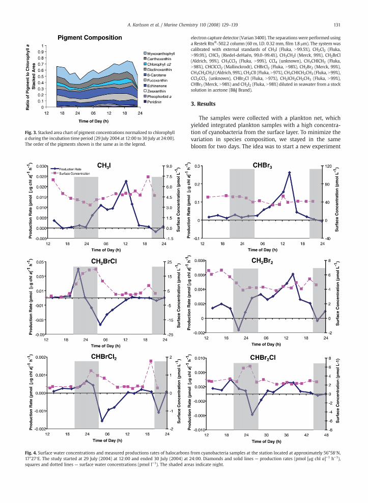
Fig. 3. Stacked area chart of pigment concentrations normalized to chlorophylla during the incubation time period (29 July 2004 at 12:00 to 30 July at 24:00).The order of the pigments shown is the same as in the legend.

Fig. 4. Surface water concentrations and measured productions rates of halocarbons17°27′E. The study started at 29 July (2004) at 12:00 and ended 30 July (2004) atsquares and dotted lines — surface water concentrations (pmol l−1). The shaded are

131A. Karlsson et al. / Marine Chemistry 110 (2008) 129–139

electron capture detector (Varian 3400). The separationswere performed usinga Restek Rtx®-502.2 column (60 m, I.D. 0.32 mm, film 1.8 μm). The systemwascalibrated with external standards of CH3I (Fluka, N99.5%), CH2Cl2 (Fluka,N99.9%), CHCl3 (Riedel-deHaën, 99.0–99.4%), CH3CH2I (Merck, 99%), CH2BrCl(Aldrich, 99%), CH3CCl3 (Fluka, N99%), CCl4 (unknown), CH3CHICH2 (Fluka,N98%), CHClCCl2 (Mallinckrodt), CHBrCl2 (Fluka, N98%), CH2Br2 (Merck, 99%),CH3CH2CH2I (Aldrich, 99%), CH2ClI (Fluka, N97%), CH3CHICH2CH3 (Fluka, N99%),CCl2CCl2 (unknown), CHBr2Cl (Fluka, N97%), CH2ICH2CH2CH3 (Fluka, N99%),CHBr3 (Merck, N98%) and CH2I2 (Fluka, N98%) diluted in seawater from a stocksolution in acetone (B&J Brand).

3. Results

The samples were collected with a plankton net, whichyielded integrated plankton samples with a high concentra-tion of cyanobacteria from the surface layer. To minimize thevariation in species composition, we stayed in the samebloom for two days. The idea was to start a new experiment

from cyanobacteria samples at the station located at approximately 56°58′N,24:00. Diamonds and solid lines — production rates (pmol [μg chl a]−1 h−1),as indicate night.

Table 1Average surface water concentrations from the entire cruise and at the cyanobacteria bloom station (pmol L−1), production/removal rates (pmol [μg chl a]−1 h−1)during day and night and total daily production rates (pmol [μg chl a]−1 day−1) for a 24 h period

Compound Entire cruise Bloom station Day Night Total daily

Mean surface water concentration andstandard deviation

Mean surface water concentration andstandard deviation

Productionrate

Productionrate

Productionrate

(pmol L−1) (pmol L−1) (pmol[μg chl a]−1 h−1)

(pmol[μg chl a]−1 h−1)

(pmol[μg chl a]−1 day−1)

CH3I 4.7±0.7 4.6±0.6 0.010 0.00088 0.17CHCl3 3.3±2.0 2.6±0.8 nd nd ndCH3CH2I 1.1±0.7 1.5±0.6 0.0026 0.0018 0.056CH2BrCl 0.87±0.80 6.2±6.5 −0.011 0.0047 −0.14CCl3CH3 6.4±0.6 5.6±0.5 nd nd ndCCl4 7.8±0.5 7.1±0.4 nd nd ndC2HCl3 5.3±2.8 2.9±0.8 nd nd ndCHBrCl2 0.44±0.11 0.46±0.27 −0.00043 0.000088 −0.0064CH2Br2 8.0±2.0 4.8±1.0 0.0036 0.0005 0.062CH2ClI 29±7.3 19±3.2 nd nd ndC2Cl4 1.0±0.2 0.90±0.21 nd nd ndCHBr2Cl 3.2±0.9 3.1±1.1 0.0019 −0.00078 0.025CHBr3 45±12 48±13 0.093 0.026 1.7

n=24 n=18

nd — not detected.


every two hours for this period in order to elucidate thediurnal cycle in the formation of halocarbons, and also to getreplicate measurements of two dark and two light periods.However, instrumental problems during the first 12 h ofstation occupation prevented sampling. Therefore, data wereavailable only from the last 36 h of the experiment.

Fig. 5. The concentration of CH3I, CHBr3, CH2BrCl and CH2Br2 in the productionexperiment.

3.1. Species composition

The investigated bloom was dominated by cyanobacteria,with the filamentous Pseudanabaena limnetica the mostabundant species. Aphanothece sp., Aphanothece parallellifor-mis, and the filamentous Aphanizomenon and Nodularia

study. Points connected with lines are measurements from one incubation


spumigena, were found to a lesser extent (Fig. 2). The twolatter are the most common bloom-forming cyanobacteria inthe Baltic Sea (HABES), but, in 2004 it was confirmed by theHelsinki Commission (HELCOM) that P. limnetica was adominating species. During our investigation the bloom wasin its latest stage, thus, the cyanobacteria might have been inan unfavorable physiological state. The other more frequentlyoccurring species were Cryptomonodales spp., Pyramimonassp., Nitzschia paleacea and dinoflagellates, but these were alltoo small to be concentrated with the plankton net.

In each incubation experiments the pigment compositionwas determined (Fig. 3). The cyanobacteria specific pigmentsmyxoxanthophyll and echinenone (Poutanen and Nikkilä,2001) were high in concentration over the incubation period.The ratio between pigments and chlorophyll a did not varysignificantly, which indicates that the species compositionduring the studied 36 h period was essentially unchanged.

The concentration of chl a in the bloomwas 5.1 μg chl a L−1,which is a representative value for blooms in the Baltic (Staland Walsby, 2000). After concentration with the plankton net,the concentration of chl a in the samples was 50 to 500 μgchl a L−1.

3.2. Determination of halocarbon production rates

Fromeach incubation series, halocarbonproduction/removalrates were calculated and normalized to chlorophyll a (Fig. 4).For some brominated (CHBr3, CH2Br2, CHBr2Cl, CH2BrCl andCH2BrCl2) and some iodinated (CH3I and CH3CH2I) halocarbons,production could be observed. The results in Fig. 4 reveal diurnalcycles for the measured halocarbons with periods of bothproduction and removal. The production rates during daylight,

Fig. 6. Depth profiles from the station at approximately 56°58′N, 17°27

night and for a whole day are summarized in Table 1 togetherwith average surface water concentrations in the investigatedarea and during the entire cruise.

CHBr3, CH2Br2, CH3I and CH3CH2I were produced mainlyduring daylight. The other brominated compounds had ratherhigh removal rates at sunrise. For CHBrCl2 and CH2BrCl thisremoval even exceeded the production, which had its max-imum late in the day or even at night. CHBr2Cl was producedduring midday which resulted in a net increase over day.

To better visualize the diurnal cycles, the concentrations ofsome halocarbons in the different incubations are shown (Fig. 5).Theproduction rates inFig. 4arebasedon6hmeasurements, andthe increase in concentrations during an experiment was notalways linear, e.g. at the transition between day and night. Al-though the different incubation series vary in chlorophyll a con-centration, the overall trend is clearer in these graphs then for theaveraged data in Fig. 4.

The surface water concentrations at the bloom stationwere similar to surfacewater concentrations during the entirecruise. The production rates for most compounds were in amagnitude of fmol [μg chl a]−1 h−1), which would have beenhard to measure without the plankton net concentration. Forsuch a low production, no enrichment of halocarbons in theupper mixed layer is expected since the loss due to air–seaexchange and turbulent eddy diffusion would dominate.

3.3. Correlation of production rates to observed surface waterconcentration

To elucidate if the compounds studied were formed bylarge sized organisms that contain chlorophyll a, such as thecyanobacteria, or small sized organisms, alternatively abiotic

′E. The rosette sampler was submerged at 21:00 30 July (UTC).

Table 2Average calculated transfer velocities (±1 standard deviation) and sea–airflux during the production study

k660 Sea→air flux

(cm h−1) (nmol m−2 day−1)

CH3I 4.1±2.2 4.3CH3CH2I 3.8±2.0 1.3CH2BrCl 3.9±2.1 8.1CHBrCl2 3.6+2.0 0.49CH2Br2 3.9+2.1 4.2CH2ClI 3.8+2.0 16CHBr2Cl 3.6+1.9 2.9CHBr3 3.6+1.9 37

U10 (m s−1).3.8±1.2.


processes, a comparison of the observed surface waterconcentration change and the surface water concentrationchange calculated from production rates was made.

The change in surface water concentration, ΔCsurface, isexpressed as

DCsurface ¼ DCprod þ DCfluxes ð1Þ

where ΔCfluxes is the change in concentration due to air–seaexchange and vertical eddy diffusion in the mixed layer (seeAppendix A). ΔCfluxes can be calculated from

DCfluxes ¼Fturbulence

h� FseaYair

h

� �� Dt ð2Þ

where F denotes the fluxes and h is the lower limit of thesampled water column. Therefore, h equals the height of theplankton net.

The depth profiles of the halocarbons in Fig. 6 showmaximaat the bottom of the mixed layer, except for CH2BrCl, whichindicate that the direction of the flux is to the atmosphere. Theconcentration in air was set to zero, since no air sampling wasperformed. This will to some extent overestimate the sea to airflux,whichwill bediscussed later. Transfer velocities during thestudy, from the sea–air exchange calculation, are summarizedin Table 2 together with the calculated daily flux.

The turbulent flux is dependent on the concentrationgradient in the mixed layer, which is determined from thedepth profiles (Fig. 6). It is assumed, that during the study thechange in concentration at depthsN10 m was negligiblecompared to the change in surface concentration.

Table 3The value of q, as defined in Eq. (7), to best describe the observed surface water co

Compound q P1day

DCsurface;observed

C0

0@

1A

CH3I 0.91 −9%CH2BrCl 0 113%CHBrCl2 0.64 −17%CH2Br2 1 −18%CHBr2Cl 0.80 −3%CHBr3 1 −14%

A high value of q indicates that the ΔCsurface,observed correlates with a chl a relaconcentration, C0, after one day, is compared to two hypothetical situations. The firstwith the plankton net (q=0) and the second case where the production is only from

The impact of production and removal on the surfacewater concentration can be expressed as

DCprod ¼ PPS þ PSWð Þ � Dt ð3Þ

where PPS is the production/removal by large sizes photosyn-thetic organisms. PSW is the production/removal by chemicalprocesses, such as photochemical reactions and hydrolysis, andalso from smaller organisms not caught in the plankton net,such as non-colony forming bacteria or small micro-algae.Production rates in the concentrated samples equals

Psample ¼PPS � chl a½ �sample

chl a½ �SWþ PSW ð4Þ

where [chl a]sample is the measured concentration of chlor-ophyll a in the sample and [chl a]SW is the concentration in thebloom (5.1 μg L−1). It is assumed that PSW is independent of theup-concentration of cyanobacteria due to the samplingprocedure. If all production originates from either PPS or PSW,ΔCprod becomes

PPS ¼ 0 ZDCprod ¼ Psample � Dt ð5Þ

PSW ¼ 0 ZDCprod ¼ Psample � chl a½ �SWchl a½ �sample

� Dt: ð6Þ

To determine the relative contribution of Eqs. (5) and (6) tothe observed surface water concentration change, ΔCsurface,
observed, the data is fitted to
DCsurface;observed ¼ DCprod þ DCfluxes

¼ q� Psample � chl a½ �SWchl a½ �sample

þ 1� qð Þ � Psample

!

�Dt þ DCfluxes:

ð7Þ

The data points derived for the calculation is the sum ofthe ΔCs from the start of the incubations to each of the
measured points. The coefficient q (0≤q≤1) is determined byleast squares regression, and describes which of the pro-cesses, PPS and PSW, best explains the observed variation insurface water concentration (Table 3). For q=0, the variationis best explained by PSW, and for q=1, the variation is bestexplained by PPS. The observed surface water concentrationsare plotted together with the calculated surface concentration
ncentration, ΔCsurface,observed

P1day

DCsurface;calc;q¼1

C0

0@

1A

P1day

DCsurface;calc;q¼0

C0

0@

1A

−38% 197%−1178% −458%−104% 215%

53% 214%−76% 271%−15% 361%

ted production, PPS. The observed change in concentration, from the startcase is if the productionwas independent of the concentration of the samplesPPS (q=1).


for a case with only PSW (q=0), only PPS (q=1) and for theoptimized fit of q in Fig. 7.

For CHBr3 and CH2Br2 the observed surface waterconcentrations are best fitted with a production related onlyto the large size fraction. To explain the observed concentra-tions of CH3I, CHBr2Cl and CHBrCl2 a production related to thesmall size fraction is required as well. For CH2BrCl, the best fitis achieved for a casewhere all production originates from thesmall size fraction. The change in concentration (in percen-tage of the start concentration) after one day is also noted inTable 3. As can be seen, all halocarbons considered, except

Fig. 7. Observed surface concentration, Csurface,observed (___), compared to concentratdiffusion), Cfluxes ( ), a hypothetical situation where all production is abiotsituation where all production is related to organisms caught in the plankton net, Cobserved surface water concentrated is presented, Cfluxes+Cprod (optimized q) ().

CH2BrCl, would be highly overestimated if the productionwould be caused by only PSW. If the assumption, from thedepth profiles, that the flux at all times is from the ocean tothe atmosphere, then, setting the air concentration to zero inthe air–sea flux calculation would lead to an even higheroverestimation. For CH2BrCl, the predicted surface waterconcentration after one day is much lower than the observed,which may indicate that the concentration in the atmosphereis significant.

A second approach to estimate the large size, cyanobacteria,related production is to consider a case where the PPS/PSW ratio

ion calculated from fluxes (air–sea exchange and mixed layer turbulent eddyic or caused by small size organisms, Cfluxes+Cprod (q=0) ( ), and, afluxes+Cprod (q=1) ( ). Also, a best fit of both of these process to the


is not constant throughout the experiment Eqs. (1), (3) and (4)can be combined to

PPS ¼DCsurface;observed�DCfluxes

Dt � Psample

� �1� chl a½ �sample

chl a½ �SW

� � ð8Þ

and

PSW ¼Psample � DCsurface;observed�DCfluxes

Dt � chl a½ �samplechl a½ �SW

� �1� chl a½ �sample

chl a½ �SW

� � : ð9Þ

The results from the calculation are shown in Fig. 8 togetherwith production rates for a hypothetical situation where the
measured production is explained only by PPS (PSW=0).
Fig. 8. PPS ( ) and PSW ( ) calculated to explain all of the vari

For CHBr3 and CH3I, the calculated PPS follows the PPS for asituation where PSW=0, which confirms that these com-pounds are produced by large size organisms in the sample.PSW fluctuates around zero production/removal and isthought to be negligible for these compounds. For CH2Br2,the calculated PPS is even higher than for a situation with noPSW. To satisfy Eq. (9), this higher PPS is balanced with anegative PSW, that is, removal related to the small size fractionmay be occurring. For CH2BrCl and CHBrCl2, PPS is negativeduring almost the entire experiment, and all production isdue to PSW. However, as noted earlier, this may be aconsequence of uncertainties in air–sea flux estimations. ForCHBr2Cl the fit of the calculated PPS to PPS (PSW=0) is slightlybetter, except in two measured points around midnightwhere a transition from positive to negative PPS (PSW=0)

ation in surface water concentrations, and PPS if PSW=0 ( ).


instead has become a transition from negative to positive PPS.This is again balanced by an opposite PSW. To summarize, theproduction of CHBr3, CH2Br2, CH3I, and to a lesser degreeCHBr2Cl, seams to originate from the large sized, cyanobac-teria, fraction, while CH2BrCl and CHBrCl2 has a bettercorrelation to the small sized fraction.

The potential error in this prediction is of coursesignificant, due to the uncertainties in the flux predictions,and a potential non-uniform production in the mixed layer.The uncertainties in the parameterization of the air–seaexchange and the turbulent mixing are large, especially whenthe atmospheric concentrations are not considered, anddepth profiles are assumed to be constant. Ideally, theseparameters would be measured throughout the study. If aproduction could be measured in non-concentrated, as wellas concentrated samples the situation would be even simpleras PPS and PSW then could be determined from

Psample;concentrated ¼ PPS � chl a½ �sample;concentrated

chl a½ �SWþ PSW

Psample;SW ¼ PPS þ PSW:

4. Discussion

The surface water concentrations are in an order ofmagnitude that could be expected for open waters intemperate areas (Quack and Wallace, 2003). The measuredproduction rates, however, are fairly low compared to otherinvestigations of natural populations. For instance, in thesouthern ocean, production rates for CHBr3 have been foundto vary between 6 and 6000 pmol [μg chl a]−1 day−1

(Abrahamsson et al., 2004). Studies of production rates ofhalocarbons by individual species are not that common andoften dealing with diatoms (e.g. Moore et al., 1996). When thecyanobacteria Synechococcus sp. was tested for the capabilityof CH3I production against other phytoplankton species, noproduction could be detected (Manley and de la Cuesta,1997).Some experiments have been performed with the red micro-alga Porphyridium purpureum, where production rates of CH3Iand CHCl3 was found to be between 0.20 and 1.2 pmol [μg chla]−1 day−1, and between 0.13 and 0.78 pmol [μg chl a]−1 day−1

respectively (Scarratt and Moore, 1999), which is in the sameorder of magnitude as for this study. One could suspect thatorganisms living in brackish waters would produce halocar-bons to a lesser extent. However, investigations of macro-algae species found both in the Baltic and on the Swedishwest coast (approximate salinity of 25) revealed that therewere no significant differences in production rates (Ekdahl,1997; Abrahamsson et al., 2003).

In order to elucidate if the production mechanism incyanobacteria is similar to that of other macro- and micro-algae, a complementary experiment was performed with a N.spumigena culture (unpublished data). Incubation experi-ments were performed with the addition of hydrogenperoxide. A dramatic increase in halocarbon production wasobserved, which indicates haloperoxidase activity, which is inagreement with the theory behind halocarbon formation inboth macro- and micro-algae (Collén et al., 1994). The findingthat cyanobacteria produce halocarbons has not to our

knowledge been shown earlier. However, an indication ofsuch a production was given by Schall et al. (1996), whoinvestigated meltponds in the Antarctica where severalhalocarbons were formed, and the dominating organismswere cyanobacteria.

The formation of halocarbons (CHBr3, CH2Br2 and CH3I)showed a diurnal variation, with highest production ataround midday (Fig. 4). This is in line with earlier studies byus where similar variations have been seen both in rock poolsand in the open ocean (Ekdahl et al., 1998; Abrahamsson et al.,2004). This also supports the possible role of enzymespossessing halperoxidase activity, since hydrogen peroxideis formed during photosynthesis. CH2BrCl, CHBrCl2 andCHBr2Cl, with production maxima later in the day and evenat night, seem not to have a direct correlation to photosynth-esis. One possibility is that they can be degradation productsof e.g. CHBr3 or CH2Br2. Also, CHBr2Cl could possibly beconverted to CHBrCl2 since it starts to degrade just prior to theproduction maxima of CHBrCl2 (Fig. 4). Additional support forthis theory is the calculated values of q, for this study(Table 3), which is a measure of the importance of a chl arelated production to the total production. The value of q, forthese brominated halocarbons, decreases in the order CHBr3,CHBr2Cl, CHBrCl2, CH2BrCl, which implies that the productionrelated to e.g. chemical processes, PSW, becomes increasinglyimportant. The rate of transformation should correlate with qfor a situation of high, chl a related, CHBr3 production as inthis study. It has been observed in the open ocean that theremoval of biogenic halocarbons is rapid, and that neither air–sea flux nor the chemical and microbial degradation ratesfound in the literature can account for the measured losses(Abrahamsson et al., 2004). In the incubation experiments,a large consumption was seen for CHBrCl2, CHBr2Cl andCH2BrCl during late night or early morning (Figs. 4 and 8). Atransformation or degradationmechanismmust be present. Ifthis is due to uptake, dehalogenation or bacterial degradationcould only be speculated, but it clearly indicates the need forfurther studies of removal pathways of halocarbons in naturalwaters.

The high concentration of cyanobacteria in the incuba-tions, indicated by chlorophyll a concentrations as high as500 μg L−1, could have had an effect on the rate of productiondue to shading, possible nutrient depletion and increased pH.Also, the incubations were performed in Pyrex® borosilicateflasks, which absorb light in the UVB region. This may havecaused lower production but it also decreased the possibilityof photochemical reactions.

5. Conclusions

CHBr3, CH3I, CH2Br2 and CHBr2Cl were found to be formed,mainly during daylight, from a cyanobacterial bloom in theBaltic proper. From correlation of production rates tovariations in surface water concentrations, it is evident thatthe production originates from the large size, cyanobacteriafraction of the seawater. Also, the othermajor species found inthe bloom are all smaller than the plankton net mesh size. Wetherefore suggest that the cyanobacteria are the main sourceof the reported production. The yearly cyanobacterial load ofhalocarbons from the Baltic can then be estimated from amaximum bloom coverage of 130000 km2 (Hansson, SMHI,


2006) with propagation calculated by a second degreepolynomial function over a bloom period of 1 month,production down to 20 m below the sea surface, an averagechlorophyll a concentration of 5 μg L−1 and using the q valuesfrom Table 3. For CHBr3, this would give a total production of0.11 Gg y−1. The production of CH3I, CH2Br2 and CHBr2Clwould be 5.6, 2.9, and 1.2 Mg y−1 respectively.

Acknowledgements

This work was supported by The Swedish ResearchCouncil for Environment, Agricultural Sciences and SpatialPlanning, FORMAS and The Marcus and MarianneWallenbergFoundation. We also thank Assoc. Prof. Angela Wulff at theDepartment of Marine Ecology, University of Gothenburg forkindly providing us with cultures of Nodularia spumigena forcomplementary studies.

Appendix A. Flux calculations

The vertical fluxes (mass area−1 time−1), that influence theconcentration in the surface water are the air–sea exchangeflux, Fsea→air, and the flux from the turbulent eddy diffusion inthe water column, Fturbulence. The change in concentration,ΔCfluxes, down to awater depth of h for a time period of Δt canbe expressed as

DCfluxes ¼Fturbulence

h� FseaYair

h

� �� Dt:

In this study, samples were takenwith a plankton net. Thedepth, h, was therefore the same as the length of this net. The
air–sea flux is calculated from
FseaYair ¼ k660 � Csurface �Cair

H

� �

where Cair is the concentration in air and H is the Henry's Lawconstant. k660 is the transfer velocity (cm h−1), which is highlydependent on the wind stress. Attempts have been made toapproximate the transfer velocity by a polynomial, up tocubic, function of thewind speed. For this study, the quadraticparameterization of Wanninkhof (1992) is used.

k660 ¼ 0:31� U210 �

ffiffiffiffiffiffiffiffiffi660Sc

r

where U10 is the wind speed at 10 m which can be estimatedfrom the logarithmic wind law for neutral conditions, bytaking the ratio to a measured value, Ud, at height d above sealevel

U10 ¼ Udln 10=z0ð Þln d=z0ð Þ

which, for measurements of Ud at low heights, predicts U10

rather well regardless of the atmospheric stability conditions(Ro and Hunt, 2007). z0 is the roughness length, which in thiscontext does not have to be accurate determined. Theinsensitivity to the parameterization of the value of z0 isnoted by Högström et. al (2006) who chose z0=2.5⁎10−4 m fortheir calculations.

The Schmidt number, Sc, is defined as

Sc ¼ ASWqSW � D

where μSW is the dynamic viscosity of seawater (ESDU, 1977)and ρSW, its density (Millero and Poisson, 1981). D (cm2 s−1) isthe diffusion coefficient which, for diffusion in water, can beapproximated from (Hayduk and Minhas, 1982)

D ¼ 1:25V0:19b

� 0:365

!� 10�8 � A

9:58Vb

�1:12

SW � T1:52k

where Tk (K) is the temperature, Vb is the molar volume (cm3

mol−1) of the solute at the normal boiling point (hereapproximated by the Le Bas method).

The turbulent flux can be calculated from the vertical eddydiffusivity, Kz, if a Fickian behaviour is assumed

Fturbulence ¼ Kz � dCdz

where z is the depth. The vertical eddy diffusivity in themixed layer can be calculated from (Denman and Gargett,1983)

Kz ¼ 0:25� ε� N�2

where ε is the rate of dissipation of turbulent kinetic energy(TKE) and N is the Brunt–Väisälä frequency

Nu

ffiffiffiffiffiffiffiffiffiffiffiffiffiffiffiffiffiffiffiffig � AqSWqSW � Az

s

where g is the acceleration of gravity. ε can be approximated(by combination of Eqs. (2) and (5) in Denman and Gargett,1983) as

εcqa � C10 � U2

10=qw� �3=2

j� h

where ρa is the density of air, κ is the Von Karman constant(=0.40), C10 is the drag coefficient (≈1.3⁎10−3).

References

Abrahamsson, K., Choo, K.S., Pedersén, M., Johansson, G., Snoeijs, P., 2003.Effects of temperature on the production of hydrogen peroxide andvolatile halocarbons by brackish-water algae. Phytochemistry 64,725–734.

Abrahamsson, K., Lorén, A., Wulff, A., Wängberg, S.-Å., 2004. Air–seaexchange of halocarbons: the influence of diurnal and regional variationsand distribution of pigments. Deep-Sea Research Part II: Topical Studiesin Oceanography 51, 2789–2805.

Asada, K., 1999. The water–water cycle in chloroplasts: scavenging of activeoxygens and dissipation of excess photons. Annual Review of PlantPhysiology and Plant Molecular Biology 50, 601–639.

Barlow, R.G., Mantoura, R.F.C., Cummings, D.G., Fileman, T.W., 1997. Pigmentchemotaxonomic distributions of phytoplankton during summer in thewestern Mediterranean. Deep-Sea Research Part II: Topical Studies inOceanography 44 (3), 833–850.

Bianchi, T.S., Engelhaupt, E., Westman, P., Andren, T., Rolff, C., Elmgren, R.,2000. Cyanobacterial blooms in the Baltic Sea: natural or human-induced? Limnology and Oceanography 45 (3), 716–726.

Collén, J., Ekdahl, A., Abrahamsson, K., Pedersén, M., 1994. The involvement ofhydrogen peroxide in the production of volatile halogenated compoundsby Meristiella gelidium. Phytochemistry 36 (5), 1197–1202.


Denman, K.L., Gargett, A.E., 1983. Time and space scales of vertical mixing andadvection of phytoplankton in the upper ocean. Limnology andOceanography 28 (5), 801–815.

Ekdahl, A., 1997. On the origin and assessment of biogenic halocarbons. Ph.D.Thesis, Göteborg University.

Ekdahl, A., Abrahamsson, K., 1997. A simple and sensitive method forthe determination of volatile halogenated organic compounds in seawater in the amol l−1 to pmol l−1 range. Analytica Chimica Acta 357 (3),197–209.

Ekdahl, A., Pedersén, M., Abrahamsson, K., 1998. A study of the diurnalvariation of biogenic volatile halocarbons. Marine Chemistry 63, 1–8.

Engineering Sciences Data Unit (ESDU), London (England), 1977. ThermalConductivity, Viscosity, Heat Capacity, Density and Prandtl Number ofSea Water and Its Concentrates. ESDU Data Items, vol. 77024. 16 pp.

Finni, T., Kononen, K., Olsonen, R., Wallström, K., 2001. The history ofcyanobacterial blooms in the Baltic Sea. Ambio 30 (4–5).

Gribble, G.W., 2004. Natural Organohalogens, Euro Chlor Science Dossier.Hansson, M., 2006. Cyanobakterieblomningar i Östersjön, resultat från

satellitövervakning 1997–2005. SMHI Oceanografi. 82.Hayduk, W., Minhas, B.S., 1982. Correlations for predictions of molecular

diffusivities in liquids. Canadian Journal of Chemical Engineering 60,295–299.

Högström, U., Smedman, A.-S., Bergström, H., 2006. Calculation of windspeed variation with height over the sea. Wind Engineering 30 (4),269–286.

Jakopitsch, C., Regelsberger, G., Furtmüller, P.G., Rüker, F., Peschek, G.A.,Obinger, C., 2001. Catalase-peroxidase from Synechocystis is capable ofchlorination and bromination reactions. Biochemical and BiophysicalResearch Communications 287, 682–687.

Kaneko, T., Sato, S., Kotani, H., Tanaka, A., Asamizu, E., Nakamura, Y., Miyajima,N., Hirosawa, M., Sugiura, M., Sasamoto, S., Kimura, T., Hosouchi, T.,Matsuno, A., Muraki, A., Nakazaki, N., Naruo, K., Okumura, S., Shimpo, S.,Takeuchi, C., Wada, T., Watanabe, A., Yamada, M., Yasuda, M., Tabata, S.,1996. Sequence analysis of the genome of the unicellular Cyanobacter-ium Synechocystis sp. Strain PCC6803. II. Sequence determination of theentire genome and assignment of potential protein-coding regions. DNAResearch 3, 109–136.

Klebanoff, S.J., 1968. Myeloperoxidase–halide–hydrogen peroxide antibacter-ial system. Journal of Bacteriology 95 (6), 2131–2138.

Manley, S.L., de la Cuesta, J.L., 1997. Methyl iodide production from marinephytoplankton cultures. Limnology and Oceanography 42 (1), 142–147.

Millero, F.J., Poisson, Alain, 1981. International one-atmosphere equation ofstate of seawater. Deep-Sea Research, Part A: Oceanographic ResearchPapers 28 (6A), 625–629.

Moore, R.M., Webb, M., Tokarczyk, R., Wever, R., 1996. Bromoperoxidase andiodoperoxidase enzymes and production of halogenatedmethanes inmarinediatom cultures. Journal of Geophysical Research 101 (C9), 20899–20908.

O'Dowd, C.D., Jimenez, J.L., Bahreini, R., Flagan, R.C., Seinfeld, J.H., Hämeri, K.,Pirjola, L., Kulmala, M., Jennings, S.G., Hoffmann, T., 2002. Marine aerosolformation from biogenic iodine emissions. Nature 417, 632–636.

Poutanen, E.L., Nikkilä, K., 2001. Carotenoid pigments as tracers ofcyanobacterial blooms in recent and post-glacial sediments of the BalticSea. AMBIO: A Journal of the Human Environment 30 (4), 179–183.

Quack, B., Wallace, D.W.R., 2003. Air–sea flux of bromoform: controls, rates,and implications. Global Biogeochemical cycles 17 (1), 1023.

Ro, K.S., Hunt, P.G., 2007. Characteristic wind speed distributions andreliability of the logarithmic win profile. Journal of EnvironmentalEngineering 133 (3), 313–318.

Rouhiainen, L., Paulin, L., Suomalainen, S., Hyytiäinen, H., Buikema, W.,Haselkorn, R., Sivonen, K., 2000. Genes encoding synthetases of cyclicdepsipeptides, anabaenopeptilides, in Anabaena strain 90. MolecularMicrobiology 37, 156–167.

Scarratt, M.G., Moore, R.M., 1999. Production of chlorinated hydrocarbonsand methyl iodide by the red microalga Porphyridium purpureum.Limnology and Oceanography 44 (3), 703–707.

Schall, C., Heumann, K.G., De Mora, S., Lee, P.A., 1996. Biogenic brominatedand iodinated organic compounds in ponds on the McMurdo Ice Shelf,Antarctica. Antarctic Science 8 (1), 45–48.

Solomon, S., Mills, M., Heidt, L.E., Pollock, W.H., Tuck, A.F., 1992. On theevaluation of ozone depletion potentials. Journal of Geophysical Research97, 825–842.

Stal, L.J., Walsby, A.E., 2000. Photosynthesis and nitrogen fixation in acyanobacterial bloom in the Baltic Sea. European Journal of Phycology 35,97–108.

van Pée, K.-H., Unversucht, S., 2003. Review— biological dehalogenation andhalogenation reactions. Chemosphere 52, 299–312.

Wagenknecht, H.-A.,Woggon,W.-D.,1997. Identification of intermediates in thecatalytic cycle of chloroperoxidase. Chemistry & Biology 4 (5), 367–372.

Wanninkhof, R., 1992. Relationship between wind speed and gas exchangeover the ocean. Journal of Geophysical Research 97 (C5), 7373–7382.

Wuosmaa, A.M., Hager, L.P., 1990. Methyl chloride transferase: a carbocationroute for biosynthesis of halometabolites. Science 249 (4965), 160–162.

Documents

Cyanobacterial blooms in the Baltic — A source of halocarbons