Cycloidal Rotor Aerodynamic and Aeroelastic Analysis

Author's pre-print copy

Cite as: Gagnon, L., Morandini, M., Quaranta, G., Muscarello, V., and Masarati, P.,

« Aerodynamic models for cycloidal rotor analysis », Aircraft Engineering and Aerospace

Technology, 2016, doi:10.1108/AEAT-02-2015-0047.

Contact Information

Dr Louis Gagnon

Postdoctoral Fellow

Dipartimento di Scienze e Tecnologie Aerospaziali, Politecnico di Milano, via La Masa 34, Milano 20156, Italy

louis.gagnon@polimi.it

+39 02 2399 8642

Prof. Marco Morandini

Assistant Professor

Dipartimento di Scienze e Tecnologie Aerospaziali, Politecnico di Milano, via La Masa 34, Milano 20156, Italy

marco.morandini@polimi.it

+39 02 2399 8362

Prof. Giuseppe Quaranta

Assistant Professor

Dipartimento di Scienze e Tecnologie Aerospaziali, Politecnico di Milano, via La Masa 34, Milano 20156, Italy

giuseppe.quaranta@polimi.it

+39 02 2399 8405

Dr Vincenzo Muscarello

Postdoctoral Fellow

Dipartimento di Scienze e Tecnologie Aerospaziali, Politecnico di Milano, via La Masa 34, Milano 20156, Italy

vincenzo.muscarello@polimi.it

+39 02 2399 8641

Prof. Pierangelo Masarati

Associate Professor

Dipartimento di Scienze e Tecnologie Aerospaziali, Politecnico di Milano, via La Masa 34, Milano 20156, Italy

pierangelo.masarati@polimi.it

+39 02 2399 8309

Cycloidal Rotor Aerodynamic and Aeroelastic Analysis

Abstract

Purpose – few modeling approaches exist for cycloidal rotors because they are a prototypal technology. Thus, new

models for their analysis were developed and validated. These models were used to analyze cycloidal rotors and a

helicopter that uses them instead of a tail rotor.

Design/methodology/approach – three different models were developed to study the aerodynamic response of cycloidal

rotors. They are a simplified analytical model resolved algebraically; a multibody model resolved numerically; and an

unsteady computational fluid dynamics (CFD) model. The models were validated using data coming from three different

experimental sources, each with rotor spans and radii of roughly 1 m. The CFD model was used to investigate the

influence of rotor arms. The efficiency and the stability of the rotor in different configurations were studied. An aeroelastic

multibody simulation was used to verify the influence of flexibility on rotor response.

Findings – the analyses suggested that cycloidal rotors can increase the efficiency of a helicopter at high velocities while

flexibility reduces it and may lead to instabilities.

Research limitations/implications – these models do not consider the effect of boundary layer friction on the trailing

vortices generated by rotor blades.

Practical implications – these models allow a four step aerodynamic optimization procedure. First, a range of optimized

configurations is obtained by the analytical model. Second, the multibody model refines that range. Third, the CFD model

detects eventual problematic blade interactions.

Originality/value – the models presented should serve researchers and industrials looking for a means to measure the

performance of cycloidal rotors concepts. The results presented also guide an initial cycloidal rotor design.

Keywords: Cycloidal rotors; Innovative cyclogyro aircrafts; Helicopter tail rotors; Computational fluid dynamics (CFD);

Multibody dynamics; Aeroelasticity

Paper type Research paper

Introduction

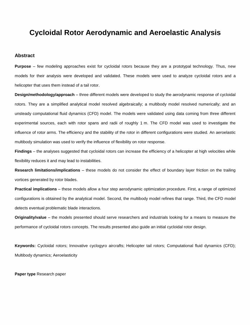
A cycloidal rotor is a device which interacts with the surrounding fluid to produce forces whose direction can be rapidly

varied. A sketch illustrates the dynamics of such a rotor in Fig. 1(a); a graphical representation is shown in Fig. 1(b). The

forces produced can take any direction in a plane normal to the axis of rotation. They have a very small latency in

response time and to some extent become increasingly efficient with airflow velocity.

Figure 1 Schematic representations of cycloidal rotors.

(a) Working principle (Benedict et al., 2013). (b) Viewed from the side.

In a cycloidal rotor, a drum carries a set of wings, or blades, whose axes are aligned with the rotation axis of the drum.

Each blade can pitch about a feathering axis which is also aligned with the rotation axis of the drum. By pitching the

blades with a period equal to that of the drum rotation, a net aerodynamic force normal to the axis of rotation is generated.

The direction of the force is controlled by changing the phase of the periodic pitch. Thus, the thrust can be vectored in a

plane without moving large mechanical parts. Cycloidal rotors have been studied for their application in vertical axis wind

and water turbines (Hwang et al., 2009; Maître et al., 2013; El-Samanoudy et al., 2010; Islam et al., 2008). Recent studies

also investigated their application in unmanned micro aerial vehicles (Jarugumilli et al., 2014; Benedict et al., 2014;

Benedict et al., 2013; Benedict et al., 2011; Benedict, 2010; Yun et al., 2007; Iosilevskii and Levy, 2006; Shrestha et al.,

2014). Nowadays, their commercial use is limited to wind turbines and marine propellers. This paper focuses on a

manned aircraft application of such rotors. A hover-capable vehicle is proposed. It makes use of a conventional helicopter

rotor for lift both in hover and forward flight, and uses one or more cycloidal rotors for anti-torque, additional propulsion,

and some control. In the explored design configuration, power demanding tasks like lift in hover and in forward flight are

delegated to a very efficient device, the main rotor.

Several researchers have experimentally explored the concept, e.g. Yun et al. (2007), IAT21 (Xisto et al., 2014), and

Bosch Aerospace as reported by McNabb (2001). They assessed the potential of cycloidal rotors to be used in large size

unmanned or small size manned vehicle propellers. Previous work by the current authors led to the development of

various models for the study of the cycloidal rotor under different configurations (Gagnon et al., 2014a, 2014b, 2014c).

The scope of this paper is to study the implementation of a cycloidal rotor as the replacement of the tail rotor on

otherwise conventional helicopters. It has been previously shown that the configuration is aerodynamically efficient

(Gagnon et al., 2014a, 2014b). This paper further studies the implementation feasibility by studying the efficiency of the

cycloidal rotor airfoils under various operating conditions. The influence of the main helicopter rotor on the rotor

aerodynamics is also discussed. A computational fluid dynamics model is used to evaluate the importance of the three-

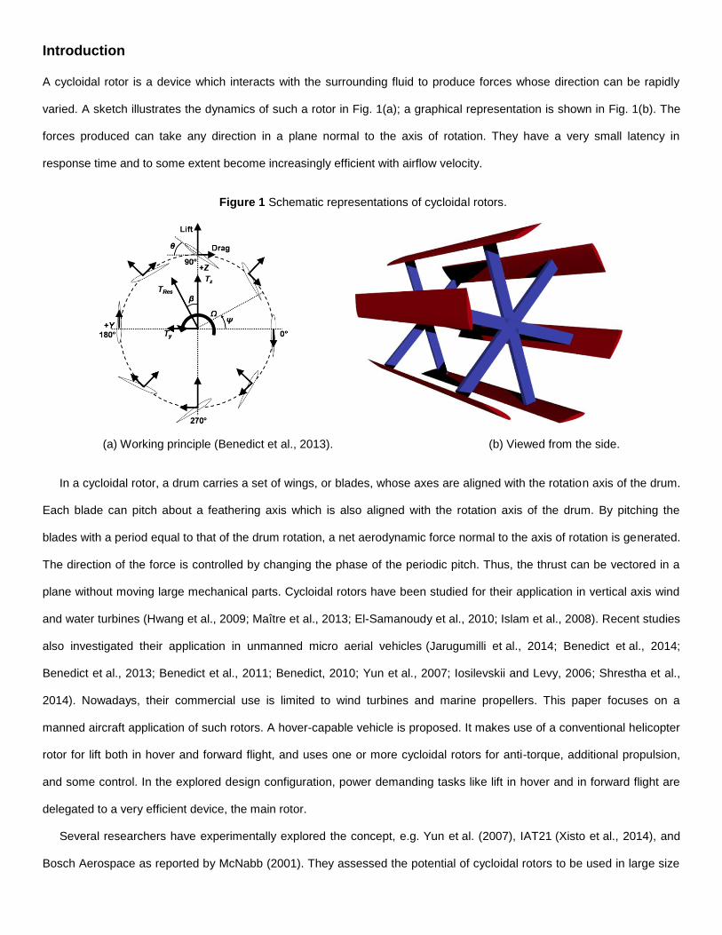
dimensionality of the rotor flow. The proposed concept is shown in Fig. 2. It was chosen after inspecting the aerodynamics

of three configurations which were reported in previous works (Gagnon et al., 2014a, 2014b).

Figure 2 Proposed helicopter concept.

This research project is part of a European effort to find an optimal use of cycloidal rotors. The objective is to study

their use in passenger carrying missions. One of the main ideas is to develop a long distance rescue vehicle which can

hover and travel at higher velocities than a traditional helicopter. Four universities and two companies constitute the

Cycloidal Rotor Optimized for Propulsion (CROP) consortium; additional information can be found on the website1.

Analytical Aerodynamic Model

Definitions

The algebraic mathematical model is used to obtain the pitching schedule required to produce the wanted thrust

magnitude and direction. It can also be used to compute the resulting thrust magnitude and direction for a given pitching

schedule. The model is also used to estimate the required power. It assumes constant slope lift coefficient and

1 http://crop-project.eu/

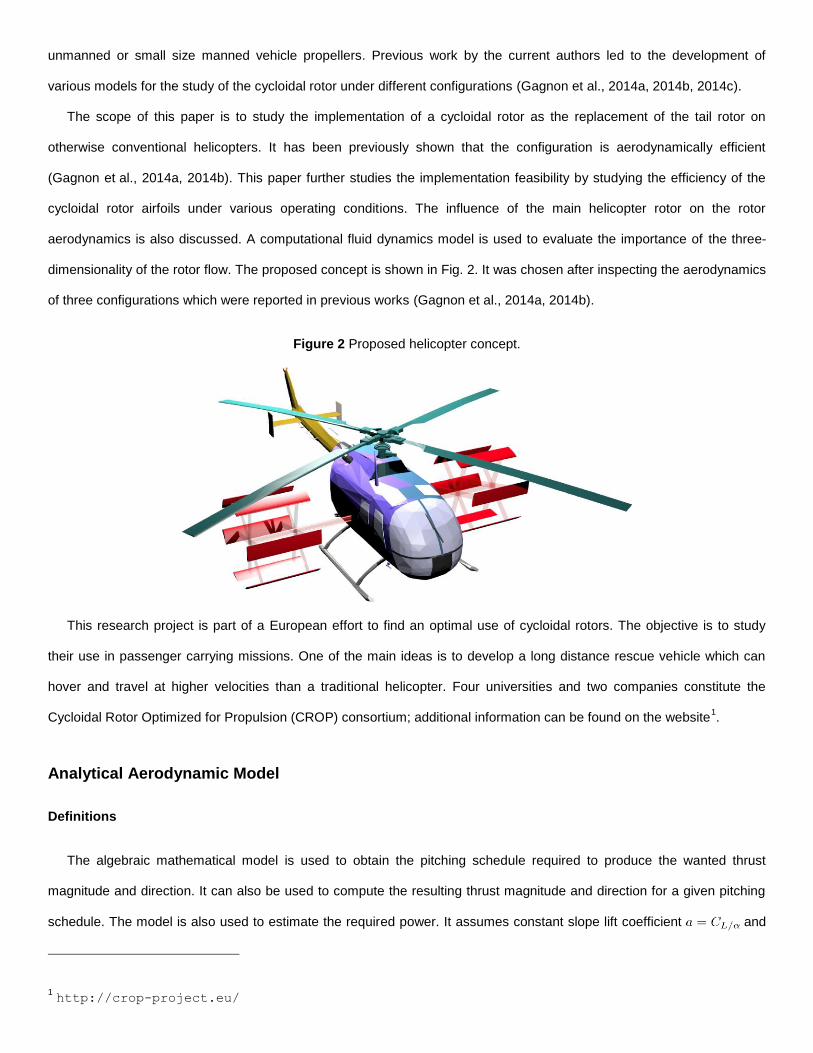
constant drag coefficient , so its use is limited to small angles of attack. It neglects blade-wake interaction. It is

convenient to specialize its solution for different flight regimes. The schematic of the model is shown in Fig. 3, which

represents the side view of the cycloidal rotor, and is in the plane of the supporting arms previously shown in Fig. 1(b).

Three different reference systems are used and are explained in Table 1.

Figure 3 Definition of reference systems.

Table 1 Description of the coordinate systems.

The thrust produced by the cycloidal rotor is shown in Fig. 3. Its direction is defined as having an angle with

respect to the axis.

Thus,

(1)

According to momentum theory, thrust produces an inflow velocity , which moves opposite to the thrust. Thus,

(2)

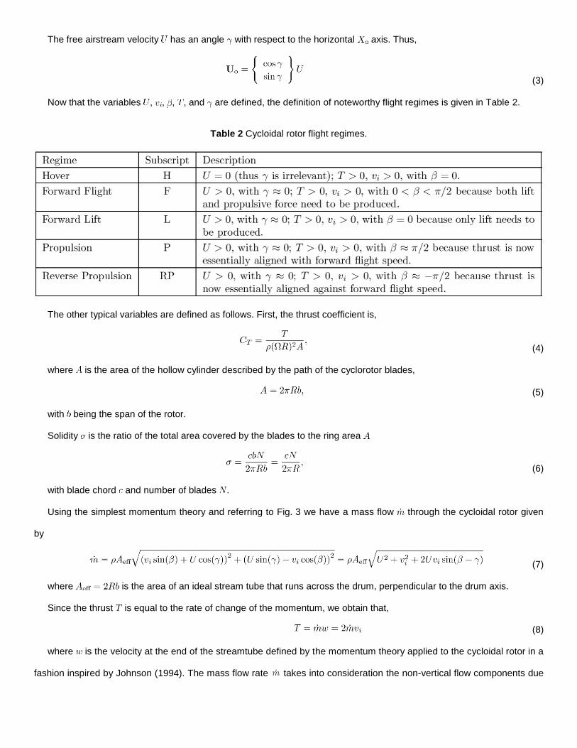
The free airstream velocity has an angle with respect to the horizontal axis. Thus,

(3)

Now that the variables , , , , and are defined, the definition of noteworthy flight regimes is given in Table 2.

Table 2 Cycloidal rotor flight regimes.

The other typical variables are defined as follows. First, the thrust coefficient is,

(4)

where is the area of the hollow cylinder described by the path of the cyclorotor blades,

(5)

with being the span of the rotor.

Solidity is the ratio of the total area covered by the blades to the ring area

(6)

with blade chord and number of blades .

Using the simplest momentum theory and referring to Fig. 3 we have a mass flow through the cycloidal rotor given

by

(7)

where is the area of an ideal stream tube that runs across the drum, perpendicular to the drum axis.

Since the thrust is equal to the rate of change of the momentum, we obtain that,

(8)

where is the velocity at the end of the streamtube defined by the momentum theory applied to the cycloidal rotor in a

fashion inspired by Johnson (1994). The mass flow rate takes into consideration the non-vertical flow components due

to the movement of the aircraft. The climb and descent velocity components do not appear in Eq. (8) because their inflow

and outflow contributions cancel each other out.

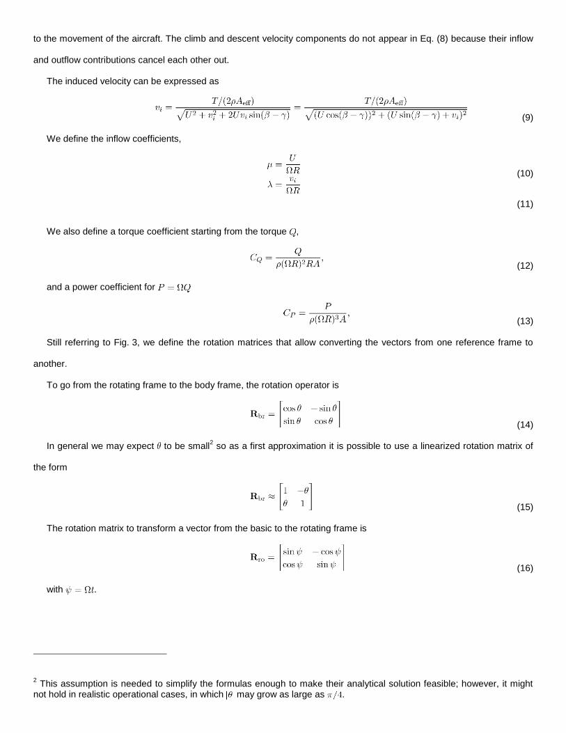
The induced velocity can be expressed as

(9)

We define the inflow coefficients,

We also define a torque coefficient starting from the torque ,

(12)

and a power coefficient for

(13)

Still referring to Fig. 3, we define the rotation matrices that allow converting the vectors from one reference frame to

another.

To go from the rotating frame to the body frame, the rotation operator is

(14)

In general we may expect to be small2 so as a first approximation it is possible to use a linearized rotation matrix of

the form

(15)

The rotation matrix to transform a vector from the basic to the rotating frame is

(16)

with .

2 This assumption is needed to simplify the formulas enough to make their analytical solution feasible; however, it might

not hold in realistic operational cases, in which may grow as large as .

(10)

(11)

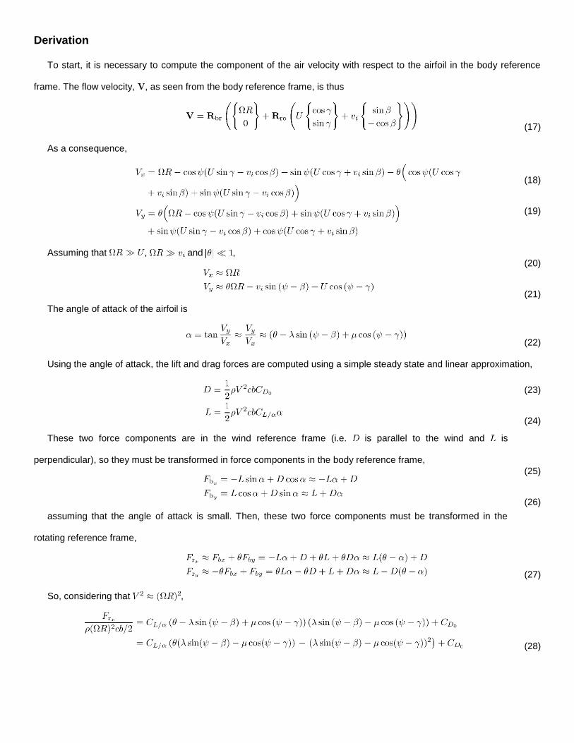
Derivation

To start, it is necessary to compute the component of the air velocity with respect to the airfoil in the body reference

frame. The flow velocity, , as seen from the body reference frame, is thus

(17)

As a consequence,

Assuming that , and ,

The angle of attack of the airfoil is

(22)

Using the angle of attack, the lift and drag forces are computed using a simple steady state and linear approximation,

These two force components are in the wind reference frame (i.e. is parallel to the wind and is

perpendicular), so they must be transformed in force components in the body reference frame,

assuming that the angle of attack is small. Then, these two force components must be transformed in the

rotating reference frame,

(27)

So, considering that ,

(28)

(18)

(19)

(20)

(21)

(23)

(24)

(25)

(26)

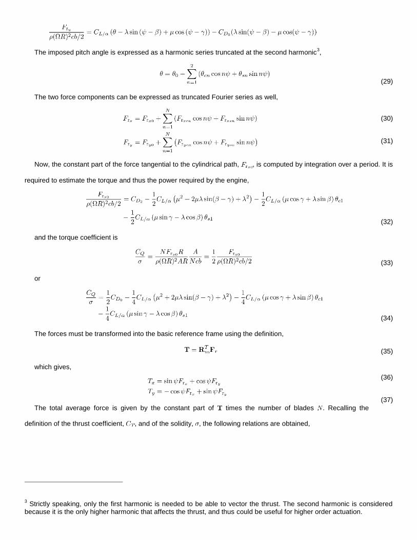
The imposed pitch angle is expressed as a harmonic series truncated at the second harmonic3,

(29)

The two force components can be expressed as truncated Fourier series as well,

Now, the constant part of the force tangential to the cylindrical path, , is computed by integration over a period. It is

required to estimate the torque and thus the power required by the engine,

(32)

and the torque coefficient is

(33)

or

(34)

The forces must be transformed into the basic reference frame using the definition,

(35)

which gives,

The total average force is given by the constant part of times the number of blades . Recalling the

definition of the thrust coefficient, , and of the solidity, , the following relations are obtained,

3 Strictly speaking, only the first harmonic is needed to be able to vector the thrust. The second harmonic is considered

because it is the only higher harmonic that affects the thrust, and thus could be useful for higher order actuation.

(30)

(31)

(36)

(37)

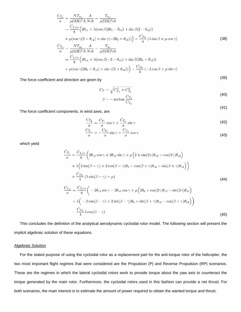
The force coefficient and direction are given by

The force coefficient components, in wind axes, are

which yield

(44)

(45)

This concludes the definition of the analytical aerodynamic cycloidal rotor model. The following section will present the

implicit algebraic solution of these equations.

Algebraic Solution

For the stated purpose of using the cycloidal rotor as a replacement part for the anti-torque rotor of the helicopter, the

two most important flight regimes that were considered are the Propulsion (P) and Reverse Propulsion (RP) scenarios.

These are the regimes in which the lateral cycloidal rotors work to provide torque about the yaw axis to counteract the

torque generated by the main rotor. Furthermore, the cycloidal rotors used in this fashion can provide a net thrust. For

both scenarios, the main interest is to estimate the amount of power required to obtain the wanted torque and thrust.

(38)

(39)

(40)

(41)

(42)

(43)

It is expected that a vertical flow component originating from the main rotor will impinge the cycloidal rotors located

below it. This component is not considered by the current model; owing to the characteristics of cycloidal rotors it is

assumed that such inflow will require a pitch angle adjustment but will not impair the efficiency of the main rotor. Another

flight condition which has not yet been considered is the use of the cycloidal rotor to contribute to the lift provided by the

main rotor when flying at low advance ratios.

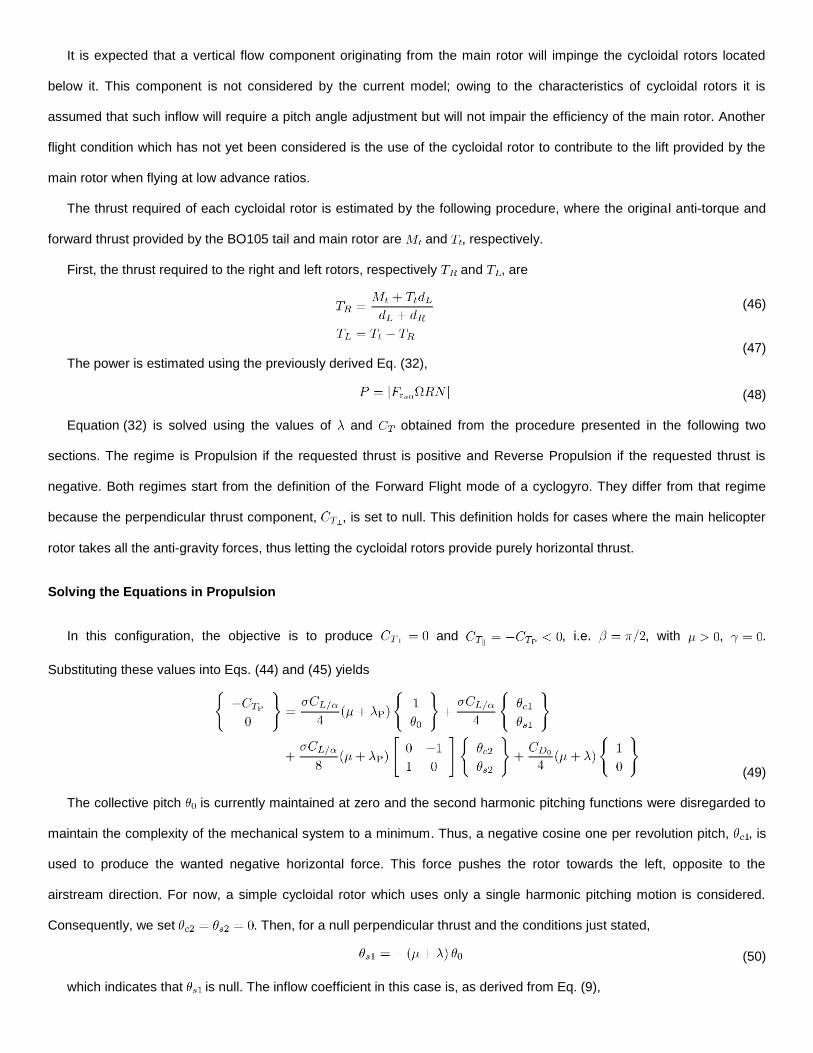
The thrust required of each cycloidal rotor is estimated by the following procedure, where the original anti-torque and

forward thrust provided by the BO105 tail and main rotor are and , respectively.

First, the thrust required to the right and left rotors, respectively and , are

The power is estimated using the previously derived Eq. (32),

(48)

Equation (32) is solved using the values of and obtained from the procedure presented in the following two

sections. The regime is Propulsion if the requested thrust is positive and Reverse Propulsion if the requested thrust is

negative. Both regimes start from the definition of the Forward Flight mode of a cyclogyro. They differ from that regime

because the perpendicular thrust component, , is set to null. This definition holds for cases where the main helicopter

rotor takes all the anti-gravity forces, thus letting the cycloidal rotors provide purely horizontal thrust.

Solving the Equations in Propulsion

In this configuration, the objective is to produce and , i.e. , with , .

Substituting these values into Eqs. (44) and (45) yields

(49)

The collective pitch is currently maintained at zero and the second harmonic pitching functions were disregarded to

maintain the complexity of the mechanical system to a minimum. Thus, a negative cosine one per revolution pitch, , is

used to produce the wanted negative horizontal force. This force pushes the rotor towards the left, opposite to the

airstream direction. For now, a simple cycloidal rotor which uses only a single harmonic pitching motion is considered.

Consequently, we set . Then, for a null perpendicular thrust and the conditions just stated,

(50)

which indicates that is null. The inflow coefficient in this case is, as derived from Eq. (9),

(46)

(47)

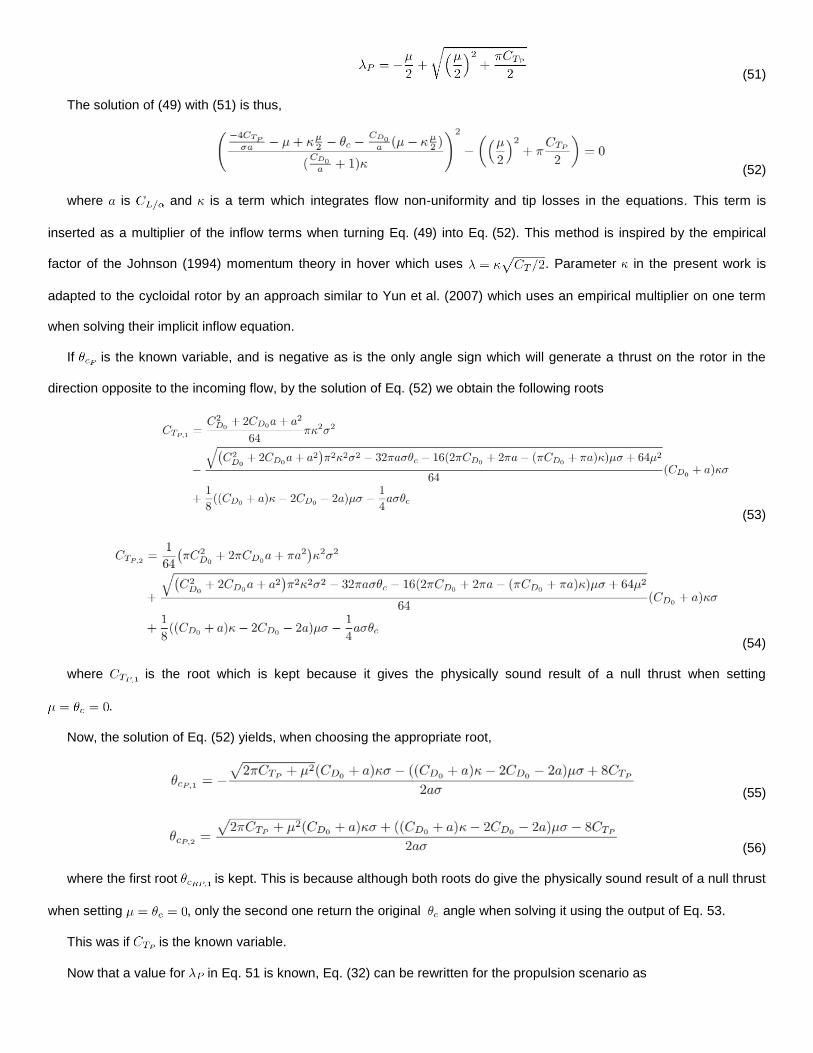
(51)

The solution of (49) with (51) is thus,

(52)

where is and is a term which integrates flow non-uniformity and tip losses in the equations. This term is

inserted as a multiplier of the inflow terms when turning Eq. (49) into Eq. (52). This method is inspired by the empirical

factor of the Johnson (1994) momentum theory in hover which uses . Parameter in the present work is

adapted to the cycloidal rotor by an approach similar to Yun et al. (2007) which uses an empirical multiplier on one term

when solving their implicit inflow equation.

If is the known variable, and is negative as is the only angle sign which will generate a thrust on the rotor in the

direction opposite to the incoming flow, by the solution of Eq. (52) we obtain the following roots

(53)

(54)

where is the root which is kept because it gives the physically sound result of a null thrust when setting

.

Now, the solution of Eq. (52) yields, when choosing the appropriate root,

(55)

(56)

where the first root is kept. This is because although both roots do give the physically sound result of a null thrust

when setting , only the second one return the original angle when solving it using the output of Eq. 53.

This was if is the known variable.

Now that a value for in Eq. 51 is known, Eq. (32) can be rewritten for the propulsion scenario as

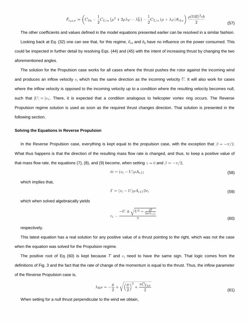
(57)

The other coefficients and values defined in the model equations presented earlier can be resolved in a similar fashion.

Looking back at Eq. (32) one can see that, for this regime, and have no influence on the power consumed. This

could be inspected in further detail by resolving Eqs. (44) and (45) with the intent of increasing thrust by changing the two

aforementioned angles.

The solution for the Propulsion case works for all cases where the thrust pushes the rotor against the incoming wind

and produces an inflow velocity which has the same direction as the incoming velocity . It will also work for cases

where the inflow velocity is opposed to the incoming velocity up to a condition where the resulting velocity becomes null,

such that . There, it is expected that a condition analogous to helicopter vortex ring occurs. The Reverse

Propulsion regime solution is used as soon as the required thrust changes direction. That solution is presented in the

following section.

Solving the Equations in Reverse Propulsion

In the Reverse Propulsion case, everything is kept equal to the propulsion case, with the exception that .

What thus happens is that the direction of the resulting mass flow rate is changed, and thus, to keep a positive value of

that mass flow rate, the equations (7), (8), and (9) become, when setting and ,

(58)

which implies that,

(59)

which when solved algebraically yields

(60)

respectively.

This latest equation has a real solution for any positive value of a thrust pointing to the right, which was not the case

when the equation was solved for the Propulsion regime.

The positive root of Eq. (60) is kept because and need to have the same sign. That logic comes from the

definitions of Fig. 3 and the fact that the rate of change of the momentum is equal to the thrust. Thus, the inflow parameter

of the Reverse Propulsion case is,

(61)

When setting for a null thrust perpendicular to the wind we obtain,

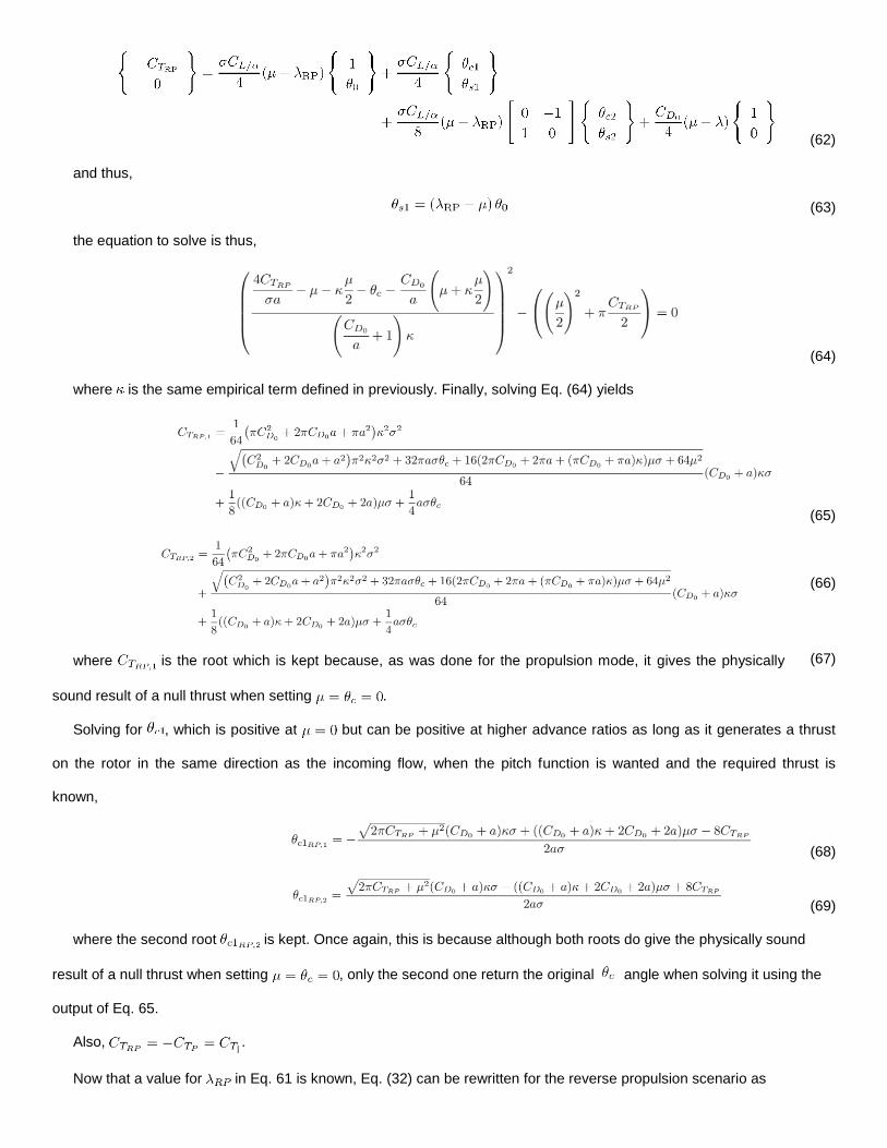
(62)

and thus,

(63)

the equation to solve is thus,

(64)

where is the same empirical term defined in previously. Finally, solving Eq. (64) yields

(65)

where is the root which is kept because, as was done for the propulsion mode, it gives the physically

sound result of a null thrust when setting .

Solving for , which is positive at but can be positive at higher advance ratios as long as it generates a thrust

on the rotor in the same direction as the incoming flow, when the pitch function is wanted and the required thrust is

known,

(68)

(69)

where the second root is kept. Once again, this is because although both roots do give the physically sound

result of a null thrust when setting , only the second one return the original angle when solving it using the

output of Eq. 65.

Also, .

Now that a value for in Eq. 61 is known, Eq. (32) can be rewritten for the reverse propulsion scenario as

(66)

(67)

(70)

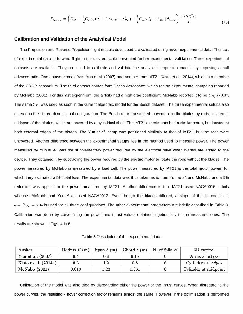
Calibration and Validation of the Analytical Model

The Propulsion and Reverse Propulsion flight models developed are validated using hover experimental data. The lack

of experimental data in forward flight in the desired scale prevented further experimental validation. Three experimental

datasets are available. They are used to calibrate and validate the analytical propulsion models by imposing a null

advance ratio. One dataset comes from Yun et al. (2007) and another from IAT21 (Xisto et al., 2014), which is a member

of the CROP consortium. The third dataset comes from Bosch Aerospace, which ran an experimental campaign reported

by McNabb (2001). For this last experiment, the airfoils had a high drag coefficient. McNabb reported it to be .

The same was used as such in the current algebraic model for the Bosch dataset. The three experimental setups also

differed in their three-dimensional configuration. The Bosch rotor transmitted movement to the blades by rods, located at

midspan of the blades, which are covered by a cylindrical shell. The IAT21 experiments had a similar setup, but located at

both external edges of the blades. The Yun et al. setup was positioned similarly to that of IAT21, but the rods were

uncovered. Another difference between the experimental setups lies in the method used to measure power. The power

measured by Yun et al. was the supplementary power required by the electrical drive when blades are added to the

device. They obtained it by subtracting the power required by the electric motor to rotate the rods without the blades. The

power measured by McNabb is measured by a load cell. The power measured by IAT21 is the total motor power, for

which they estimated a 5% total loss. The experimental data was thus taken as is from Yun et al. and McNabb and a 5%

reduction was applied to the power measured by IAT21. Another difference is that IAT21 used NACA0016 airfoils

whereas McNabb and Yun et al. used NACA0012. Even though the blades differed, a slope of the lift coefficient

is used for all three configurations. The other experimental parameters are briefly described in Table 3.

Calibration was done by curve fitting the power and thrust values obtained algebraically to the measured ones. The

results are shown in Figs. 4 to 6.

Table 3 Description of the experimental data.

Calibration of the model was also tried by disregarding either the power or the thrust curves. When disregarding the

power curves, the resulting hover correction factor remains almost the same. However, if the optimization is performed

considering only power, the value changes significantly, yielding an excellent match for the power at the cost of

mispredicting the thrust. The calibration of used for plotting Figs. 4 to 6 was conducted by giving an equally important

weight to thrust and power.

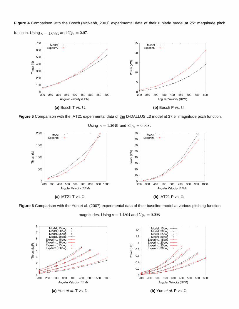
Figure 4 Comparison with the Bosch (McNabb, 2001) experimental data of their 6 blade model at 25° magnitude pitch

function. Using and .

(a) Bosch T vs. . (b) Bosch P vs. .

Figure 5 Comparison with the IAT21 experimental data of the D-DALLUS L3 model at 37.5° magnitude pitch function.

Using and .

(a) IAT21 T vs. . (b) IAT21 P vs. .

Figure 6 Comparison with the Yun et al. (2007) experimental data of their baseline model at various pitching function

magnitudes. Using and .

(a) Yun et al. T vs. . (b) Yun et al. P vs. .

Although various weightings between power and thrust were tested, it was decided to give them equal importance.

Optimizing with a strong weight on power gave an excellent match for power, but yielded a very high , which is the only

variable that is calibrated by the optimization. The smaller correctors required for the IAT21 and McNabb experimental

data may be due to the fact that their experimental model had full cylinders which are known to reduce the three-

dimensionality of the flow. To verify this hypothesis, a previously developed three-dimensional fluid dynamics

model (Gagnon et al., 2014c) is used to confirm the influence of the use of endplates on the rotor. A short description of

the model along with the computed effect of the endplates is presented in the following paragraph.

The OpenFOAM CFD toolkit has been relied upon to perform the fluid dynamic calculations. A laminar non-viscous

solver is relied on since the main contributors to the thrust are the pressure induced forces. A double mesh interface

which allows one to model a fixed angular velocity rotor zone and six embedded periodically oscillating zones has been

developed. A moving no-slip boundary condition was also developed to constrain the normal component of the fluid

velocity at the foil to match the airfoil velocity while letting the parallel velocity uninfluenced. The timestep used for the

simulations is variable and set to follow a Courant number of about 10. An inflow velocity of roughly 1 cm/s was imposed

to the whole top boundary of the domain while the bottom boundary allowed only for exiting flow. Changes of the inflow

velocity were shown to have no influence on the results when testing with a 2D grid of similar dimensions. The domain

size was 20~rotor diameters in each axis. The mesh used without endplates has 366k cells while the one with endplates

has 926k cells. The reason for such a big discrepancy is the difficulty of the snappyHexMesh meshing software to mesh

surfaces close to interfaces and the thus related need to have a highly refined mesh in these zones. The spacing between

endplates and foils is one tenth of the chord length, which is reported by Calderon et al. (2013) to have the same effect as

if it were attached to the foil.

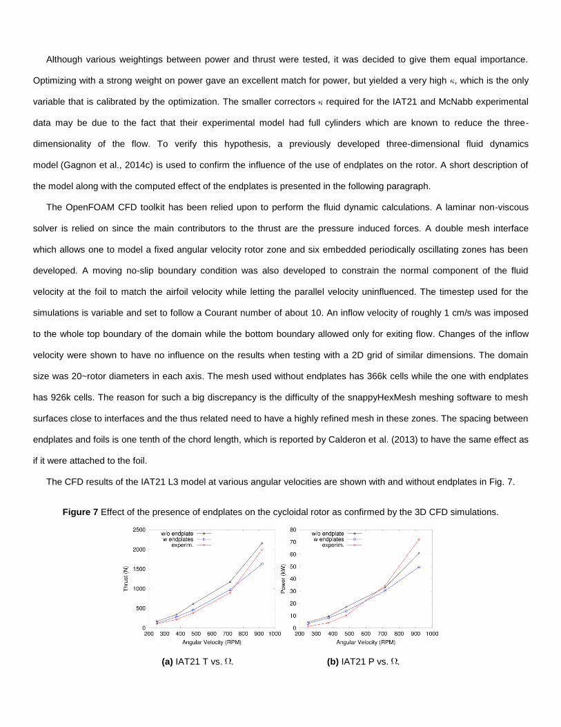
The CFD results of the IAT21 L3 model at various angular velocities are shown with and without endplates in Fig. 7.

Figure 7 Effect of the presence of endplates on the cycloidal rotor as confirmed by the 3D CFD simulations.

(a) IAT21 T vs. . (b) IAT21 P vs. .

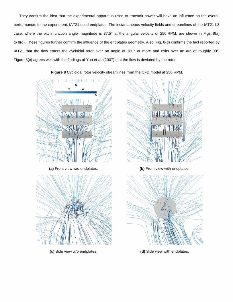
They confirm the idea that the experimental apparatus used to transmit power will have an influence on the overall

performance. In the experiment, IAT21 used endplates. The instantaneous velocity fields and streamlines of the IAT21 L3

case, where the pitch function angle magnitude is 37.5° at the angular velocity of 250 RPM, are shown in Figs. 8(a)

to 8(d). These figures further confirm the influence of the endplates geometry. Also, Fig. 8(d) confirms the fact reported by

IAT21 that the flow enters the cycloidal rotor over an angle of 180° or more and exits over an arc of roughly 90°.

Figure 8(c) agrees well with the findings of Yun et al. (2007) that the flow is deviated by the rotor.

Figure 8 Cycloidal rotor velocity streamlines from the CFD model at 250 RPM.

(a) Front view w/o endplates. (b) Front view with endplates.

(c) Side view w/o endplates. (d) Side view with endplates.

Modified Analytical and Multibody Models

Two other quickly solvable models were developed for the purpose of studying the behavior of a potential manned

vehicle which uses cycloidal rotors. One consists of a slight modification of the previous analytical model which can still be

solved algebraically. The second model is a rigid multibody dynamics system consisting of a main rotating drum and a set

of blades having a common pitching schedule comprised of a collective pitch and a first harmonic pitch. These two models

are validated against a set of three different experimental results.

Modified Analytical Model

In the previously presented analytical model, the equations were solved using only one parameter, , which allowed

calibrating the results to the experimental data quite well. The mathematics used made it so that the power and thrust

were each influenced differently by the adjustment factor. However, in this revised solution, an additional factor is used

and deemed necessary in order to compare the multibody and analytical solutions using the same mathematical basis. It

consists of the drag coefficient of the airfoil. This theory is used following the findings of McNabb (2001). He reported that

the actual viscous drag of the airfoil used for the experimental validation of his cycloidal rotor model was more than

10 times greater than the theoretical one. This new approach is also confirmed by the multibody model. Thus, the

modified analytical model uses an implementation of the inflow correction factor closer to the one of Johnson (1994). We

thus have and where is a multiplication factor for the drag coefficient.

Multibody Model

The multibody model consists of a parametric implementation of a N blade cycloidal rotor. The analysis is performed

using the MBDyn open-source multibody tool4. Inflow is calculated using momentum theory and the blade lift and drag

forces are calculated using tables for drag and lift coefficients. Here, the factor is applied to coefficients coming from

data tables and is optimized to fit the multibody model to the experimental data. The model is run until a periodic solution

is obtained; the resulting performance is obtained by averaging over the last complete rotation of the drum.

Comparison with Experimental Data

These two models are calibrated for optimal and ; the results are plotted in Figs. 9 to 11. The calibration of with

each experimental data set was done by curve fitting the thrust and power values obtained from the algebraic model. The

multibody parameter was then calibrated similarly while maintaining the algebraically obtained . In all cases, an equal

4 http://www.mbdyn.org/, last accessed September 2014.

calibration importance was given to both thrust and power. The difference noted in the power plots is explained by the fact

that at higher angles of attack the analytical model is less influenced by the drag coefficient due to its fixed value.

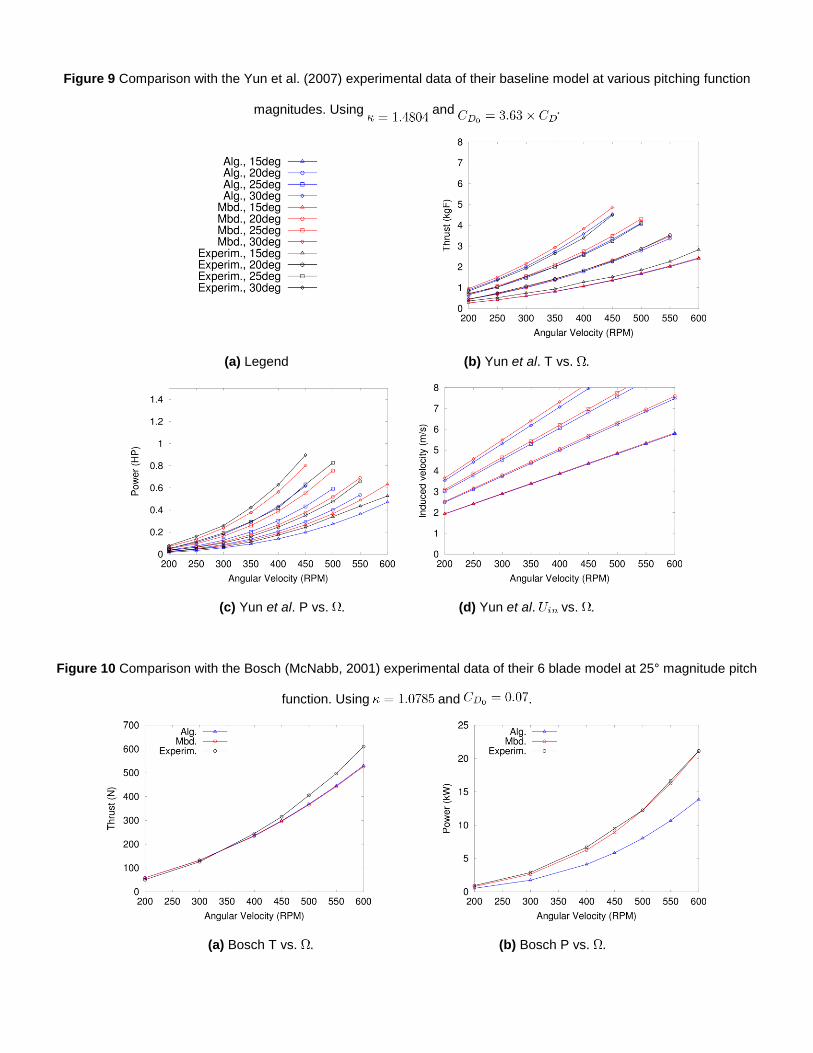
Figure 9 Comparison with the Yun et al. (2007) experimental data of their baseline model at various pitching function

magnitudes. Using and .

(a) Legend (b) Yun et al. T vs. .

(c) Yun et al. P vs. . (d) Yun et al. vs. .

Figure 10 Comparison with the Bosch (McNabb, 2001) experimental data of their 6 blade model at 25° magnitude pitch

function. Using and .

(a) Bosch T vs. . (b) Bosch P vs. .

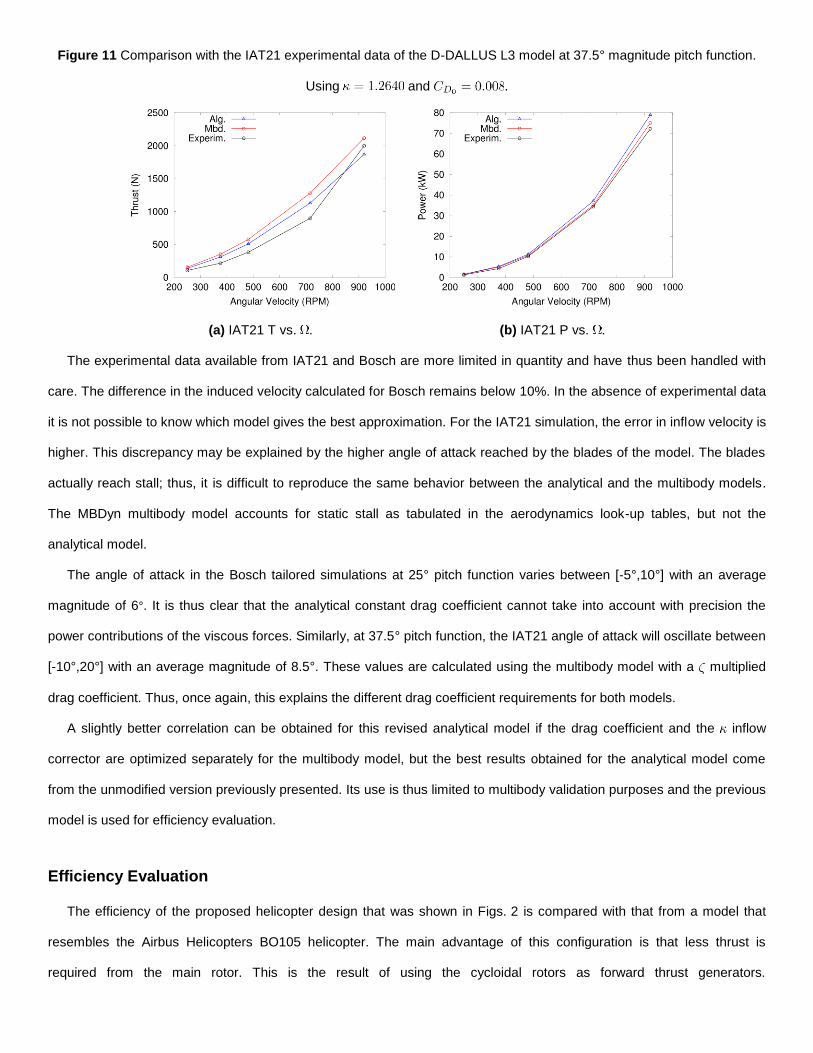
Figure 11 Comparison with the IAT21 experimental data of the D-DALLUS L3 model at 37.5° magnitude pitch function.

Using and .

(a) IAT21 T vs. . (b) IAT21 P vs. .

The experimental data available from IAT21 and Bosch are more limited in quantity and have thus been handled with

care. The difference in the induced velocity calculated for Bosch remains below 10%. In the absence of experimental data

it is not possible to know which model gives the best approximation. For the IAT21 simulation, the error in inflow velocity is

higher. This discrepancy may be explained by the higher angle of attack reached by the blades of the model. The blades

actually reach stall; thus, it is difficult to reproduce the same behavior between the analytical and the multibody models.

The MBDyn multibody model accounts for static stall as tabulated in the aerodynamics look-up tables, but not the

analytical model.

The angle of attack in the Bosch tailored simulations at 25° pitch function varies between [-5°,10°] with an average

magnitude of 6°. It is thus clear that the analytical constant drag coefficient cannot take into account with precision the

power contributions of the viscous forces. Similarly, at 37.5° pitch function, the IAT21 angle of attack will oscillate between

[-10°,20°] with an average magnitude of 8.5°. These values are calculated using the multibody model with a multiplied

drag coefficient. Thus, once again, this explains the different drag coefficient requirements for both models.

A slightly better correlation can be obtained for this revised analytical model if the drag coefficient and the inflow

corrector are optimized separately for the multibody model, but the best results obtained for the analytical model come

from the unmodified version previously presented. Its use is thus limited to multibody validation purposes and the previous

model is used for efficiency evaluation.

Efficiency Evaluation

The efficiency of the proposed helicopter design that was shown in Figs. 2 is compared with that from a model that

resembles the Airbus Helicopters BO105 helicopter. The main advantage of this configuration is that less thrust is

required from the main rotor. This is the result of using the cycloidal rotors as forward thrust generators.

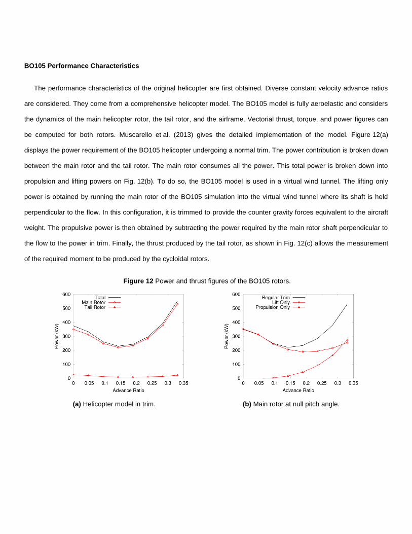
BO105 Performance Characteristics

The performance characteristics of the original helicopter are first obtained. Diverse constant velocity advance ratios

are considered. They come from a comprehensive helicopter model. The BO105 model is fully aeroelastic and considers

the dynamics of the main helicopter rotor, the tail rotor, and the airframe. Vectorial thrust, torque, and power figures can

be computed for both rotors. Muscarello et al. (2013) gives the detailed implementation of the model. Figure 12(a)

displays the power requirement of the BO105 helicopter undergoing a normal trim. The power contribution is broken down

between the main rotor and the tail rotor. The main rotor consumes all the power. This total power is broken down into

propulsion and lifting powers on Fig. 12(b). To do so, the BO105 model is used in a virtual wind tunnel. The lifting only

power is obtained by running the main rotor of the BO105 simulation into the virtual wind tunnel where its shaft is held

perpendicular to the flow. In this configuration, it is trimmed to provide the counter gravity forces equivalent to the aircraft

weight. The propulsive power is then obtained by subtracting the power required by the main rotor shaft perpendicular to

the flow to the power in trim. Finally, the thrust produced by the tail rotor, as shown in Fig. 12(c) allows the measurement

of the required moment to be produced by the cycloidal rotors.

Figure 12 Power and thrust figures of the BO105 rotors.

(a) Helicopter model in trim. (b) Main rotor at null pitch angle.

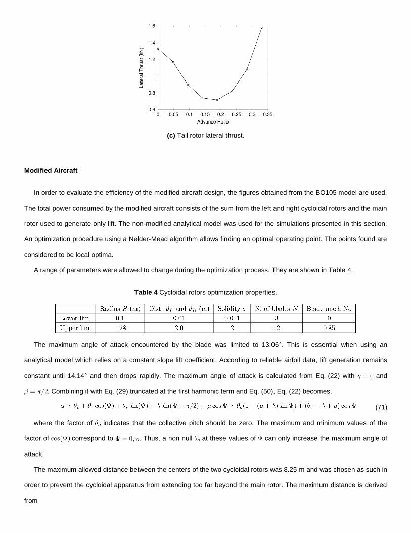
(c) Tail rotor lateral thrust.

Modified Aircraft

In order to evaluate the efficiency of the modified aircraft design, the figures obtained from the BO105 model are used.

The total power consumed by the modified aircraft consists of the sum from the left and right cycloidal rotors and the main

rotor used to generate only lift. The non-modified analytical model was used for the simulations presented in this section.

An optimization procedure using a Nelder-Mead algorithm allows finding an optimal operating point. The points found are

considered to be local optima.

A range of parameters were allowed to change during the optimization process. They are shown in Table 4.

Table 4 Cycloidal rotors optimization properties.

The maximum angle of attack encountered by the blade was limited to 13.06°. This is essential when using an

analytical model which relies on a constant slope lift coefficient. According to reliable airfoil data, lift generation remains

constant until 14.14° and then drops rapidly. The maximum angle of attack is calculated from Eq. (22) with and

. Combining it with Eq. (29) truncated at the first harmonic term and Eq. (50), Eq. (22) becomes,

(71)

where the factor of indicates that the collective pitch should be zero. The maximum and minimum values of the

factor of correspond to . Thus, a non null at these values of can only increase the maximum angle of

attack.

The maximum allowed distance between the centers of the two cycloidal rotors was 8.25 m and was chosen as such in

order to prevent the cycloidal apparatus from extending too far beyond the main rotor. The maximum distance is derived

from

(72)

where m is the main rotor diameter, is the width of the skids, and and are the lateral distances

between the edge of the helicopter lateral leg and the center of the left and right cycloidal rotors, respectively. Each rotor

uses NACA0012 airfoils; the rotor radii were limited to avoid contact with the ground or the main rotor. The maximum tip

velocity at maximum forward velocity was limited to Mach 0.85.

No longer having to provide forward thrust, the main rotor, does not require its shaft to be tilted forward. In this design,

the main rotor only pitches in order to balance the center of mass offset. The angular velocity of the cycloidal rotors was

allowed to vary when changing advance ratio or flight regime. This would make sense if they were powered, for example,

by electric motors. It is reasonable to assume that the angular velocity of the rotors could be controlled independently and

vary with the advance ratio. The pitch was restrained to single harmonic variation. The two cycloidal rotors had identical

geometry in one case and different geometries in the other. The optimization process also led to the realization that, in

order to keep a larger chord, the blade number has to be minimized. Thus, it could be set to for the further

optimization steps. The resulting vehicle is not larger than the original helicopter since it was chosen to constrain the

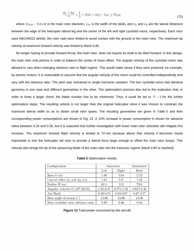
maximum lateral width so as to obtain small rotor spans. The resulting geometries are given in Table 5 and their

corresponding power consumptions are shown in Fig. 13. A 10% increase in power consumption is shown for advance

ratios between 0.25 and 0.35, but it is expected that further investigation with lower main rotor velocities will mitigate this

increase. The maximum forward flight velocity is limited to 72 m/s because above that velocity it becomes nearly

impossible to trim the helicopter tail rotor to provide a lateral force large enough to offset the main rotor torque. This

velocity also brings the tip of the advancing blade of the main rotor into the transonic regime (Mach 0.85 is reached).

Table 5 Optimization results.

Figure 13 Total power consumed by the aircraft.

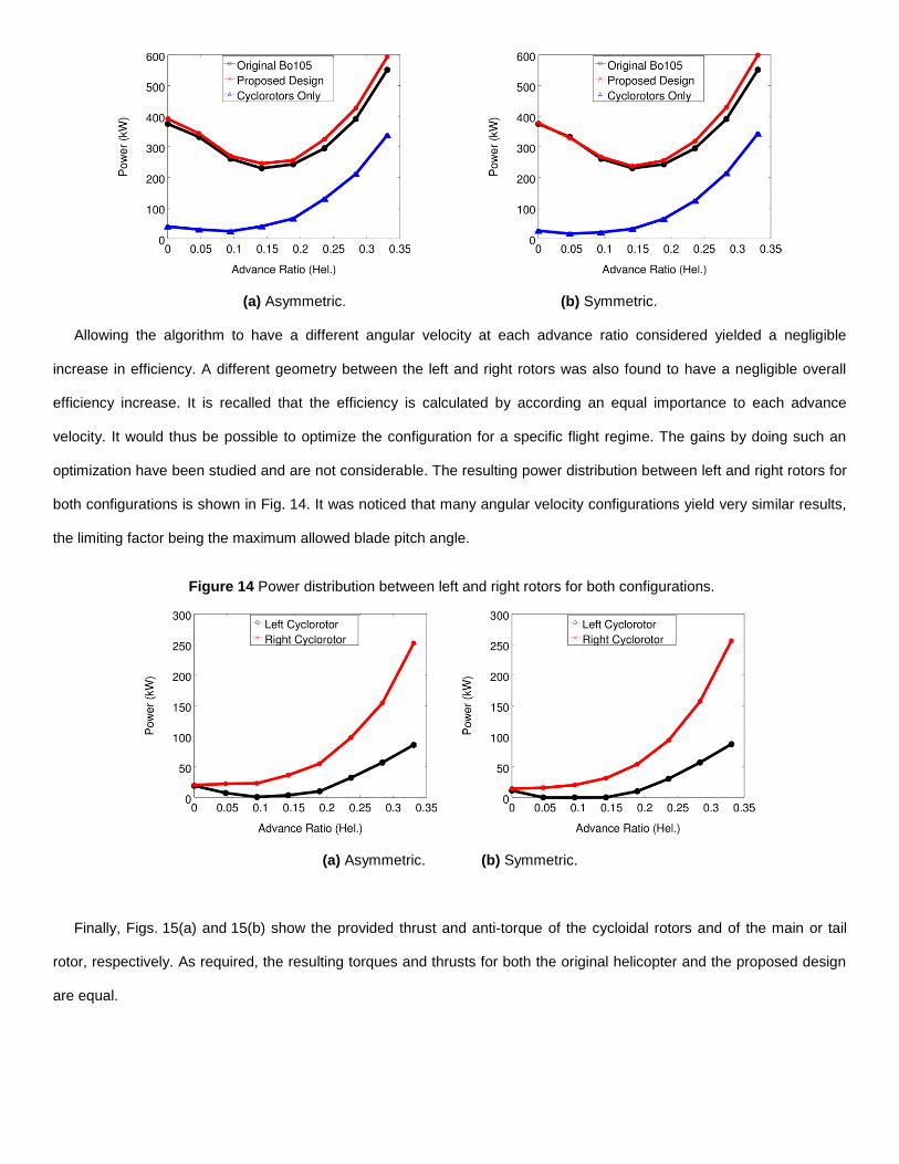
(a) Asymmetric. (b) Symmetric.

Allowing the algorithm to have a different angular velocity at each advance ratio considered yielded a negligible

increase in efficiency. A different geometry between the left and right rotors was also found to have a negligible overall

efficiency increase. It is recalled that the efficiency is calculated by according an equal importance to each advance

velocity. It would thus be possible to optimize the configuration for a specific flight regime. The gains by doing such an

optimization have been studied and are not considerable. The resulting power distribution between left and right rotors for

both configurations is shown in Fig. 14. It was noticed that many angular velocity configurations yield very similar results,

the limiting factor being the maximum allowed blade pitch angle.

Figure 14 Power distribution between left and right rotors for both configurations.

(a) Asymmetric. (b) Symmetric.

Finally, Figs. 15(a) and 15(b) show the provided thrust and anti-torque of the cycloidal rotors and of the main or tail

rotor, respectively. As required, the resulting torques and thrusts for both the original helicopter and the proposed design

are equal.

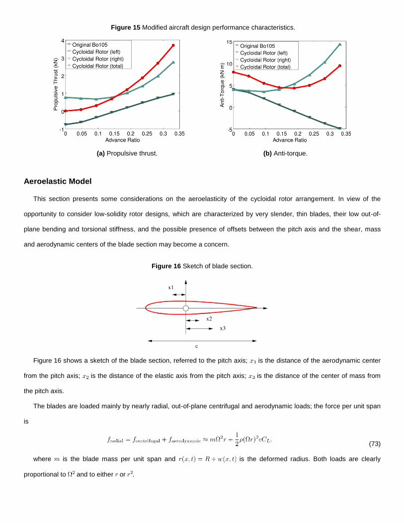
Figure 15 Modified aircraft design performance characteristics.

(a) Propulsive thrust. (b) Anti-torque.

Aeroelastic Model

This section presents some considerations on the aeroelasticity of the cycloidal rotor arrangement. In view of the

opportunity to consider low-solidity rotor designs, which are characterized by very slender, thin blades, their low out-of-

plane bending and torsional stiffness, and the possible presence of offsets between the pitch axis and the shear, mass

and aerodynamic centers of the blade section may become a concern.

Figure 16 Sketch of blade section.

Figure 16 shows a sketch of the blade section, referred to the pitch axis; is the distance of the aerodynamic center

from the pitch axis; is the distance of the elastic axis from the pitch axis; is the distance of the center of mass from

the pitch axis.

The blades are loaded mainly by nearly radial, out-of-plane centrifugal and aerodynamic loads; the force per unit span

is

(73)

where is the blade mass per unit span and is the deformed radius. Both loads are clearly

proportional to and to either or .

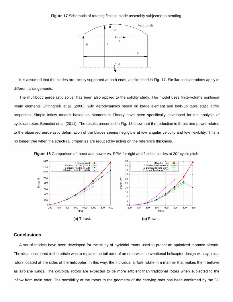
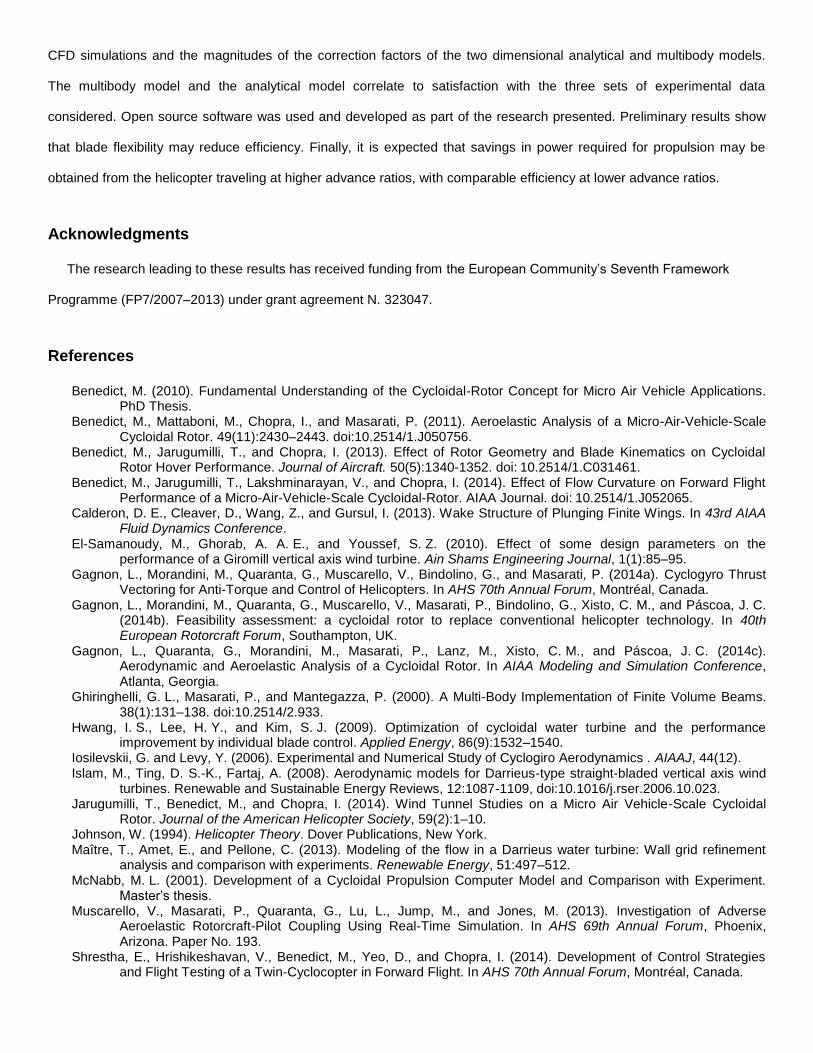
Figure 17 Schematic of rotating flexible blade assembly subjected to bending.

It is assumed that the blades are simply supported at both ends, as sketched in Fig. 17. Similar considerations apply to

different arrangements.

The multibody aeroelastic solver has been also applied to the solidity study. The model uses finite-volume nonlinear

beam elements Ghiringhelli et al. (2000), with aerodynamics based on blade element and look-up table static airfoil

properties. Simple inflow models based on Momentum Theory have been specifically developed for the analysis of

cycloidal rotors Benedict et al. (2011). The results presented in Fig. 18 show that the reduction in thrust and power related

to the observed aeroelastic deformation of the blades seems negligible at low angular velocity and low flexibility. This is

no longer true when the structural properties are reduced by acting on the reference thickness.

Figure 18 Comparison of thrust and power vs. RPM for rigid and flexible blades at 20° cyclic pitch.

(a) Thrust. (b) Power.

Conclusions

A set of models have been developed for the study of cycloidal rotors used to propel an optimized manned aircraft.

The idea considered in the article was to replace the tail rotor of an otherwise conventional helicopter design with cycloidal

rotors located at the sides of the helicopter. In this way, the individual airfoils rotate in a manner that makes them behave

as airplane wings. The cycloidal rotors are expected to be more efficient than traditional rotors when subjected to the

inflow from main rotor. The sensibility of the rotors to the geometry of the carrying rods has been confirmed by the 3D

CFD simulations and the magnitudes of the correction factors of the two dimensional analytical and multibody models.

The multibody model and the analytical model correlate to satisfaction with the three sets of experimental data

considered. Open source software was used and developed as part of the research presented. Preliminary results show

that blade flexibility may reduce efficiency. Finally, it is expected that savings in power required for propulsion may be

obtained from the helicopter traveling at higher advance ratios, with comparable efficiency at lower advance ratios.

Acknowledgments

The research leading to these results has received funding from the European Community’s Seventh Framework

Programme (FP7/2007–2013) under grant agreement N. 323047.

References

Benedict, M. (2010). Fundamental Understanding of the Cycloidal-Rotor Concept for Micro Air Vehicle Applications. PhD Thesis.

Benedict, M., Mattaboni, M., Chopra, I., and Masarati, P. (2011). Aeroelastic Analysis of a Micro-Air-Vehicle-Scale Cycloidal Rotor. 49(11):2430–2443. doi:10.2514/1.J050756.

Benedict, M., Jarugumilli, T., and Chopra, I. (2013). Effect of Rotor Geometry and Blade Kinematics on Cycloidal Rotor Hover Performance. Journal of Aircraft. 50(5):1340-1352. doi: 10.2514/1.C031461.

Benedict, M., Jarugumilli, T., Lakshminarayan, V., and Chopra, I. (2014). Effect of Flow Curvature on Forward Flight Performance of a Micro-Air-Vehicle-Scale Cycloidal-Rotor. AIAA Journal. doi: 10.2514/1.J052065.

Calderon, D. E., Cleaver, D., Wang, Z., and Gursul, I. (2013). Wake Structure of Plunging Finite Wings. In 43rd AIAA Fluid Dynamics Conference.

El-Samanoudy, M., Ghorab, A. A. E., and Youssef, S. Z. (2010). Effect of some design parameters on the performance of a Giromill vertical axis wind turbine. Ain Shams Engineering Journal, 1(1):85–95.

Gagnon, L., Morandini, M., Quaranta, G., Muscarello, V., Bindolino, G., and Masarati, P. (2014a). Cyclogyro Thrust Vectoring for Anti-Torque and Control of Helicopters. In AHS 70th Annual Forum, Montréal, Canada.

Gagnon, L., Morandini, M., Quaranta, G., Muscarello, V., Masarati, P., Bindolino, G., Xisto, C. M., and Páscoa, J. C. (2014b). Feasibility assessment: a cycloidal rotor to replace conventional helicopter technology. In 40th European Rotorcraft Forum, Southampton, UK.

Gagnon, L., Quaranta, G., Morandini, M., Masarati, P., Lanz, M., Xisto, C. M., and Páscoa, J. C. (2014c). Aerodynamic and Aeroelastic Analysis of a Cycloidal Rotor. In AIAA Modeling and Simulation Conference, Atlanta, Georgia.

Ghiringhelli, G. L., Masarati, P., and Mantegazza, P. (2000). A Multi-Body Implementation of Finite Volume Beams. 38(1):131–138. doi:10.2514/2.933.

Hwang, I. S., Lee, H. Y., and Kim, S. J. (2009). Optimization of cycloidal water turbine and the performance improvement by individual blade control. Applied Energy, 86(9):1532–1540.

Iosilevskii, G. and Levy, Y. (2006). Experimental and Numerical Study of Cyclogiro Aerodynamics . AIAAJ, 44(12). Islam, M., Ting, D. S.-K., Fartaj, A. (2008). Aerodynamic models for Darrieus-type straight-bladed vertical axis wind

turbines. Renewable and Sustainable Energy Reviews, 12:1087-1109, doi:10.1016/j.rser.2006.10.023. Jarugumilli, T., Benedict, M., and Chopra, I. (2014). Wind Tunnel Studies on a Micro Air Vehicle-Scale Cycloidal

Rotor. Journal of the American Helicopter Society, 59(2):1–10. Johnson, W. (1994). Helicopter Theory. Dover Publications, New York. Maître, T., Amet, E., and Pellone, C. (2013). Modeling of the flow in a Darrieus water turbine: Wall grid refinement

analysis and comparison with experiments. Renewable Energy, 51:497–512. McNabb, M. L. (2001). Development of a Cycloidal Propulsion Computer Model and Comparison with Experiment.

Master’s thesis. Muscarello, V., Masarati, P., Quaranta, G., Lu, L., Jump, M., and Jones, M. (2013). Investigation of Adverse

Aeroelastic Rotorcraft-Pilot Coupling Using Real-Time Simulation. In AHS 69th Annual Forum, Phoenix, Arizona. Paper No. 193.

Shrestha, E., Hrishikeshavan, V., Benedict, M., Yeo, D., and Chopra, I. (2014). Development of Control Strategies and Flight Testing of a Twin-Cyclocopter in Forward Flight. In AHS 70th Annual Forum, Montréal, Canada.

Xisto, C. M., Páscoa, J. C., Leger, J. A., Masarati, P., Quaranta, G., Morandini, M., Gagnon, L., Wills, D., and Schwaiger, M. (2014). Numerical modelling of geometrical effects in the performance of a cycloidal rotor. In 6th European Conference on Computational Fluid Dynamics, Barcelona, Spain.

Yun, C. Y., Park, I. K., Lee, H. Y., Jung, J. S., and H., I. S. (2007). Design of a New Unmanned Aerial Vehicle Cyclocopter. Journal of the American Helicopter Society, 52(1).