D-76128 Karlsruhe, Germany - KITna.math.kit.edu/alefeld/download/1993_The_Cholesky_method_for... · , D-76128 Karlsruhe, Germany ... analysis and matrix theory (Section 2), ... LINEAR

The Cholesky Method for Interval Data

G. Alefeld and G. Mayer

Institutfür Angewandte MathematikUniversität KarZsruhe

Postfach 6980, D-76128 Karlsruhe, Germany

Dedicated to U. Kulisch on the occasion oi his 60th birthday

Submitted by Richard A. Brualdi

ABSTRACT

We apply the well-known Cholesky method to bound the solutions of linearsystems with symmetrie matriees and right-hand sides both of whieh are varyingwithin given intervals. We derive eriteria to-guarantee the feasibility and the optimal-ity of the method. Furthermore, we diseuss some general properties.

1. INTRODUCTION

It is weIl known that the fonnulae of the Gaussian algorithm can be usedto bound the solutions of the linear systems for which the coefficient matricesand the right-hand sides are varying within given intervals; see [11], or [3] and[13], where also criteria for the feasibility of this method can be found. Amethod which can be used systematically for linear systems with arealsymmetrie and positive definite point matrix is the Cholesky method. Com-pared with Gaussian elimination, it has among others certain advantages withrespect to the amount of work which has to be perfonned.

The purpose of the present paper is to investigate the Cholesky methodsystematicaIly when applied to systems with interval data. To OUfknowledgethis has not been done before. After repeating some basic facts from intervalanalysis and matrix theory (Section 2), we introduce the interval Choleskymethod in Section 3. Aseries of properties which may hold is illustrated byexamples. In Section 4 we derive several sufficient criteria for the method tobe feasible, and we prove some additional properties.

LINEAR ALGEBRA AND ITS APPLICATIONS 194:161-182 (1993) 161

@ Elsevier Seienee Publishing Co., Ine., 1993655 Avenue of the Amerieas, New York, NY 10010 0024-3795/93/$6.00

162 G. ALEFELD AND G. MAYER

2. PRELIMINARIES

By Rn, Rn x n, IR, IR n, IR nxn we denote the set of real vectors with ncomponents, the set of real n X n matrices, the set of intervals, the set ofinterval vectors with n components, and the set of n X n interval matrices;respectively. By "interval" we always mean areal compact interval. We writeinterval quantities in brackets with the exception of point quantities Ci.e.,degenerate interval quantities), which we identify with the element whichthey contain. Examples are the- null matrix 0 and the identity matrix 1. Weuse the notation [A] = [.:1, A] = ([aij]) = ([Qij' aij]) E IRnXn simultane-ously without further reference, and we proceed similarly for the elements ofRn, Rnxn, IR, and mn. We write 0 S for the tightest interval enclosure of agiven bounded sub set S ~ Rn and call it the interval hull of S.

By A > 0 we denote a nonnegative n X n matrix, i.e., aij > 0 fori,j = 1,..., n. We call x E Rn positive, writing x > 0, if Xi > 0, i =1,..., n.

We also mention the standard notation from interval analysis [3, 13]:

l[a]1 := max{lällä E [a]} = max{IQI,laI}

(absolute value), and

< [a]) ,~ min{lällä E [a]} ~ {;in{IQI, lai}if 0 $. La],otherwise

(minimal absolute value) for intervals [al For [A] E IRnXn we obtain

I[A]/ ERn x n by applying I. Ientrywise, and we deHne the comparison matrix([AJ) = (Ci) E RnXn by setting

:=

(

-I [aij ] I

Cij <[a;;])

if i =1=j,

if i = j.

Since real numbers can be viewed as degenerate intervals, I. land ( . > canalso be used for them.

By znXn we denote the set of real n X n matrices with nonpositiveoff-diagonal entries, by det A we mean the determinant of a matrix A ERnxn, and by p(A) we denote its spectral radius.

In Seetion 4 we will consider several classes of matrices A ERn x n for

CHüLESKY METHüD FüR INTERVAL DATA 163

whieh we reeall the definitions (cf. [5, 8, 17]):

A is an M-matrix if A is nonsingular, A -1 ~ 0, and A E znXn.

A is a Stieltjes matrix if A is asymmetrie M-matrix.A is an H-matrix if ( A> is an M-matrix.

A is diagonally dominant if

n

la..1 ~ ~ la..!,.. '-' ')

j=lj i=i

i = 1,..., n. (2.1)

A is strictly diagonally dominant if (2.1) holds with strict inequality.A is irreducibly diagonally dominant if A is irredueible and if (2.1) holds

with strict inequality for at least one index i.A is totally positive (totaIly nonnegative) if eaeh minor of A is positive

(nonnegative).A is an oscillatory matrix if it is totaIly nonnegative and if at least one of

its powers A k is totally positive.An interval matrix [A] E IR n x n is termed an M-matrix if each element

A E [A] is an M-matrix. In the same way the term "H-matrix" ean beextended to IRn xn. It is easy to verify that

[A] is an M-matrix if and only if ~ is an M-matrix and aij < 0 for i =1=j, andthat

[A] is an H-matrix if and only if ([ A]) is an M-matrix.

To prove these two statements one ean refer to a very useful eriterion forM-matriees due to Fan [6]:

LEMMA2.1. Let A E zn Xn. Then A is an M-matrix if and only if thereexists a positive vector x ERn sueh that Ax > O.

We reeall now some well-known results for symmetrie positive definitematriees.

LEMMA2.2. 1f A ERn xn is a symmetrie matrix, then the followingproperties are equivalent:

Ci) The matrix A is positive definite.(ii) Eaeh principal submatrix of A has a positive determinant.(iü) Eaeh eigenvalue of A is positive.

LEMMA2.3 (Cf. [5, p. 141]). A E Rnxn is a Stieltjes matrix if and onlyifA is asymmetrie and positive definite element of zn X n.

LEMMA2.4 (Cf. [7, p. 127]). 1fA E RnXn is asymmetrie and positivedefinite tridiagonal matrix, then Ais an H-matrix. .


We equip m, IRn, IRnxn with the usual real intelVal arithmetic asdescribed e.g. in [3, 11, 13]. We also assume that the reader is familiar withthe properties of this arithmetic. We only mention the formulae (cf. [3], [13])

I [:] [b]1= ([:D l[b]1

I[a]:t [b]1 ~1[a]1 +1[b]1

if 0 (/= [a],(2.2)

for intelVals [a], [b], and we recall the definitions

M:= {~Ia E [a]} for 0 ~ Q (2.3)

and

[at := {a2la E [an. (2.4)

Instead of M we also write [a]1/2.

3. THE INTERVAL CHOLESKY METHOD

Westart this seetion by specifYing the problem which we want to attack.

Let [A] E mnxn be an intelVal matrix satisfYing [A] = [A]T. Furthermore,let [b] E IRn be given. We want to bound the solution set

Ssym:= {xIAx = b, A E [A], A = AT, b E [b n (3.1)

by an intelVal vector [x].

Such a vector can be obtained by using an iterative method as describedin [3] or by applying the intelVal Gaussian algorithm, which also can be foundin [3]. Since we are only interested in bounds for the solutions of linearsystems with symmetrie coefficient matrices A, we can hope to succeed alsowith an intelVal analogue of the Cholesky method which needs approximatelyhalf the operations of the intelVal Gaussian algorithm. By this analogue, wemean the construction of an intelVal vector [x]C = ICh([A], [b]) byapplyingthe following algorithm, which we divide into three steps. To formulate themwe require [A] = [A]T, and we assume that all the steps are feasible. This

CHOLESKY METHOD FOR INTERVAL DATA 165

means that no division by an interval which contains zero appears, and that allsquare roots can be taken. Conditions which guarantee this feasibility will bederived in Seetion 4.

INTERVALCHOLESKYMETHOD.

Step 1. "LLT decomposition":

for j := 1 to n do[ljj] := ([ajj] - Ei:i [ljk]2)1/2;for i := j + 1 to n do

[lij] := ([aij] - Ei:i [lik][ljk])/[ljj];

Step 2. Forward substitution:for i := 1 to n do

[yJ:= ([bi] - L~:Ulij][Yj])/[lJ;

Step 3. Backward substitution:for i := n downto 1 do

[xJc := ([yJ - Ld~i+l [lji][xjf)/[lii];ICh([A],[b]) := [x] .

(3.2)

As usual, sums with an upper bound smaller than the lower one are;Jet';~ e ;J I-~ h.o ~o r ~ 'rho S,.,n ar o s ;n Sl-o", 1 a..a a,,,,ln al-ar1 h y a",,,,l,,;nr< th°U 1111 U ~v IJ~ Lv V. .LUv 'iu. v u' ""'Y.L 'v v..uu. ~v"'" LI YY'JU'& 'v

interval square function (2.4), which yields for arbitrary [a] E IR the inclu-sion

[ a]2 ~ [a] . [a] with equality if and only if 0 $. int([ a]) . (3.3)

We recall that we only intend to enclose -the solutions for the symmetrie

matrices contained in [A]. This justifies the use of the squares [ljd2 asdefined in (2.4) in step 1 above.

As can be seen from the formulae in the interval Cholesky method, thefeasibility of this method is independent of the right-hand side [b]. There-fore, the existence of ICh([A], [b]) is also independent of [b]. Subsequently,we will simply write ,,[x f exists" if we mean that ICh([ A], [b]) exists for anyvector [b] E IRn.

The three steps in the interval Cholesky method correspond to the threesteps of the ordinary Cholesky method for a given symmetrie matrix A E


Rn X n (provided that the feasibility is guaranteed):

Ci) Decompose A into A = LLT with a lower triangular matrix L satisfy-ing lii > 0, i = 1,. . . , n.

(ü) Solve Ly = b.(üi) Solve LTx = y.

As is weIl known, the decomposition in Ci)is unique.

Denne [L] as the lower triangular matrix with [lij] from step 1 of theinterval Cholesky method. By the inclusion monotonieity of interval arith-metie it is clear that L from Ci)exists and is eontained in [L] for eaeh matrix

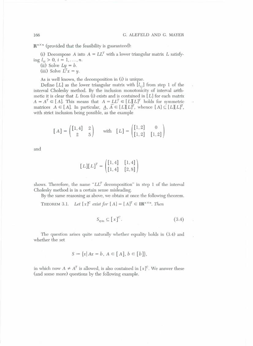
A = AT E [A]. This means that A = LLT E [L][L]T holds for symmetriematrices A E [A]. In partieular, =.1,A E [L][L]T, whenee [A] ~ [L][L]T,with strict inclusion being possible, as the example

[A] = ([1;4] :) with [L] =(

[1, 2]

[1,2] [l~ 2] )

and

[L][L]T =(

[1,4]

[1,4]

[1,4]

)[2,8]

shows. Therefore, the name" LLT deeomposition" in step 1 of the intervalCholesky method is in a certain sense misleading.

By the same reasoning as above, we obtain at onee the foIlowing theorem.

THEOREM 3.1. Let [x]C exist for [A] = [A]T E IRnXn. Then

Ssym~ [x]c. (3.4)

The question arises quite naturally whether equality holds in (3.4) andwhether the set

S := {x IAx = b, A E [A], b E [b]},

in which now A =I=- AT is allowed, is also eontained in [xf. We answer these

(and some more) questions by the foIlowing example.

CHOLESKY METHOD FüR INTERVAL DATA 167

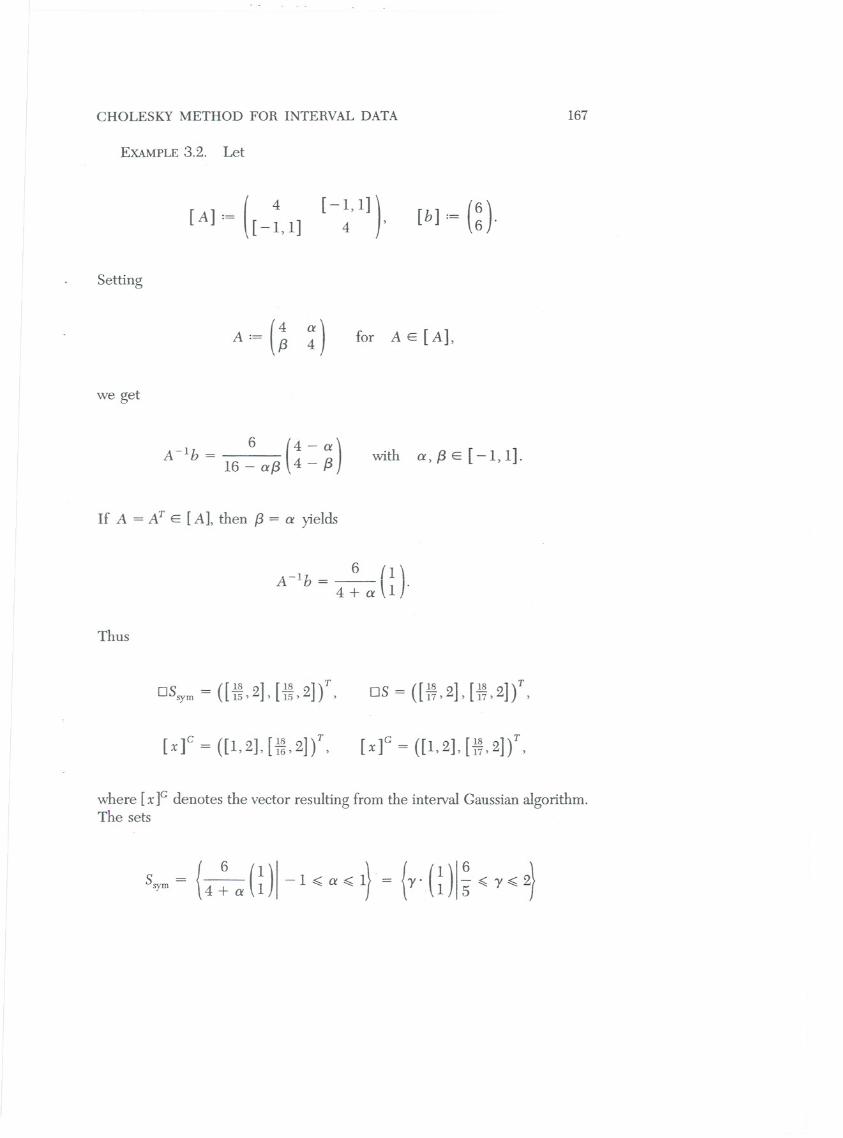
EXAMPLE3.2. Let

[A]'~ ([-~.l]

[-1,1]

)4 ' [b] := (~).

Setting

A:=(~ ~) for A E [A],

we get

A -lb - 6(

4 - a

)16 - aß 4 - ßwith a, ß E [ - 1, 1].

If A = AT E [A], then ß = a yields

A-lb = 4: a (i ).

Thus

OS - ([18 2] [18 ])T

sym - 15' , 15,2 , OS = ([i~,2], [i~, 2]f,

[ x ] c = ([ 1, 2], [ i~ ' 2] ) T , [x f = ([1,2], [ i~' 2]f,

where [x JGdenotes the vector resulting from the interval Gaussian algorithm.The sets

Ssym={4:aU)I-1<a<1} = {y'U)I~<Y<2}


y

2

S"ym

1

x1 2

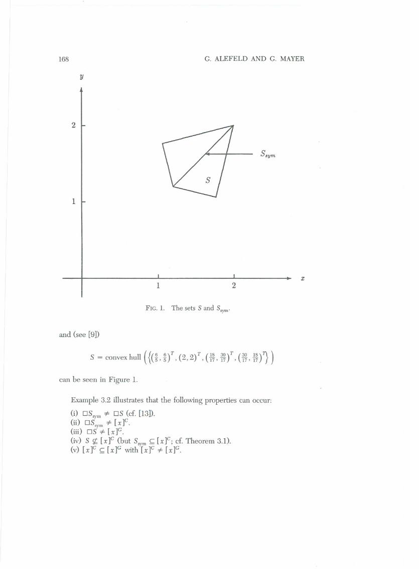
FIG. 1. The sets S and Ssym.

and (see [9])

S = convex hull ({( ~ ' ~) T , (2, 2) T , ( ~~, i~) T , ( ~, ~~)J)can be seen in Figure 1.

Example 3.2 illustrates that the following properties can occur:

Ci) OSsym"* os (cE.[13]).(ii) OSsym"* [x]C.(iii) OS"* [x]G.

(iv) S rJ,[x]C (but Ssym~ [x]C; cf. Theorem 3.1).(v) [x]C ~ [x]G with [x]C "* [x]G.


We enlarge this list by another property which is also possible:

(vi) [x]G ~ [x]G with [x]G * [x]C.

Our next example illustrates this property.

EXAMPLE3.3. Let

(

[1,4]

[ A]:= [0, 1]

[0,1]

)3 ' [ b] := ([ 0~2d .

Then [x]G = ([0.25,3], [-1, 1])T c [xf = ([0,3], [-1, I])T.

The reason why these two examples above work is best seen by expressing[ x f and [x]G in terms of the input data. One obtains

c 1

(

[a ]

)[X2] = 2 [b2] - ~[bl] ,

[a22] - [aI2] /[au] [au]

, I rb 1 r 1 \

[ ]c = .1 ! L IJ - Lal2J [ f~Xl ~ \~ ~ X2 J'

[X2]G = 1([b2] - [aI2] [bI]

),

[a22] - [aI2][aI2]/[aU] [au]

G 1{

G

}[Xl] = -[ ]

[bI] - [aI2][x2] .au

Hence, by (3.3), we always get [x2f ~ [x2]G. If, however, 0 ft. int([aI2]),then [x 2f = [x 2]G,and the subdistributivity of the interval arithmetic causes[x I]G ~ [x 1f. Similar phenomena can appear in higher dimensions, too.

We now turn to an alternative representation of [ x f. As with the result ofthe interval Gaussian algorithm (cf. e.g. [2] or [15]), the vector Ieh([ A], [b])can be expressed as a product of certain diagonal matrices [Ds], s = 1,...,n,


and lower triangular matrices [U], s = 1,.. ., n - 1, which are defined by

[d:j] .~ U/[l,,]

(l:j] .~ C [I;,]

if i=j=Fs,

if i=j=s,otherwise,

(3.5)

if i = j,

if i > j = s,otherwise.

By executing the steps 2 and 3 of the interval Cholesky algorithm, one getsthe proof of the following theorem.

THEOREM3.4. Let the elements of [Ds], [U] E mnXn be defined as in(3.5). Then for the vectors [y] and [x JCof (3.2) we get

[y] = [Dn]([Ln-I]([Dn-I](-.. ([L2]([D]\[LI]([DIHb]))))... ))),

(3.6)

[ x]c =

[D1] ([ LIt ([ D2] (... ([U-2t (rDn-I]([U-I t ([ DnHy]))))... ))).

(3.7)

Note that the parentheses cannot be omitled in general, since themultiplication of interval matrices is not associative. For point matrices[A] == A, the matrices [DS] ==DS and [U] ==U are point matrices, too.Hence, for a point vector [b] == b we get

y = DnDn-I{D-(n-I)U-1Dn-I}Dn-2

x {D-(n-2)u-2Dn-2} ... DI{ D-1 L1D1}b

= DnDn-l ... Dlfn-lin-2 ... Db

= I5ib (3.8)


with D-s:= ( Ds ) -l 15:= DnDn-l ... D2D1 fs:= D-sUDs and i:=, "in-I... i2[1. In (3.8) we used the fact that DS commutes with U for r > s

because of the particular shape of DS and U. By the same reasoning, we get

x = Dl(Ll/ D2(L2)T ... Dn-l(Ln-l)T Dny

= {Dl(Ll)TDl} {D2(L2/D2} ... {Dn-l(U-l)TDn-l} (Dn)2ib

= Üib, (3.9)

where Ü := {D1(L1)TD1}{D2(L2)TD2}... {Dn-l(Ln-l)TDn-l}(Dn)2.

Since i is a low~r triangula~ ma~rix with ones in its diagonal, the sameholds for its inverse L -1. Thus L -1 U-1 = A is the LU decomposition of Aresulting from the Gaussian algorithm without permuting rows or columns.This well-known relation between the Cholesky decomposition and the LUdecomposition of A cannot be generalized to nondegenerate interval matri-ces [A], again because the multiplication of interval matrices is not associa-tive. In addition, inverses of such matrices do not exist in the usual algebraicsense.

We end trus section with a different description of step 1 in the intervalCholesky method.

DEFINITION 3.5. Let either [A] = ([au]) E IR1X 1 or

I

[ A] =(

[au]

[e]

[eY

)

'

[ A']

= [AY E mnxn, n> 1, [e] E IRn-l, [A'] E IR(n-l)X(n-l).

(a) I[A]:= [A'] - (1/[au])[c][e]T E m(n-l)X(n-l) is termed the Schurcomplement (of the (1,1) entry [au]) provided n > 1 and 0 $. [au]. In the

product [c][c]T we assume that [cJ[cJ is evaluated as [CJ2 [see (2.4)]. I[A] isnot defined if n = 1 or if 0 E [au].

(b) We call the pair ([L],[L]T) the Cholesky decomposition of [A] if

0< Qu and if either n = 1 and [L] = (~) or

[L] =

~[c]

~

0

[L'] "(3.10)

where ([L'], [L']T) is the Cholesky decomposition oE ~[A]'


Definition 3.5(a) is a modification of the Schur complement defined in[13, p. 155], where the square of an interval [a] is computed as [a] . [a].

THEOREM3.6. The matrix [L] in (3.2) exists if and onZyif [L] from(3.10) exists. In this case, the two matrices are identicaZ.

Proof. We prove the assertion by induction with respect to the numbern of rows or columns of [ A].

If n = 1, the assertion follows from ~ ~ = [au] for 0 ~ Qu.Let the assertion be true for some n, and choose [A] from IR(n+l)X(n+l).

For ease of argumentation we replace [L], [I.:] in Definition 3.5 by [M],[M'].

Assurne first that [L] exists, where [L] is computed by the intervalCholesky method (3.2). We show that [A] has the Cholesky decomposition([M], [MY) satisfYing [M] = [L]. Since [L] exists, we obtain Qll > O.Hence [Zn] = [mn] for i = 1,. . . , n + l.

For j > 2, the formulae in the interval Cholesky method can be reformu-lated as

(

j-l

)

1/2

[Zjj] = ([ajj] - [zjd2) - k~) Zjk]2

(

' r ..]2 \ j-l \1/2

~ \[aJj] - ~~ J - '~2[lj,]2J

((

[]2

)

'-1

)

1/2

= [ajj] - [;:1] - :~2[ljk]2 ,

(3.11)

1

(

j-l

)Pij] = -[Z.. ] ([aij] - [ln][ZjlD - E [Zid[ljd

)} k = 2

1

( (

[an][ ajl]

)

j - 1

)

= -[Z.. ] [aij] - [] - E [Zid[ljk] .}} au k=2

These formulae can be interpreted as the interval Cholesky method appliedto LrA]E IRnxn,which results in a lower triangular matrix [L']. By thehypotheses made for this induction, the matrix [M'] of Definition 3.5(b)exists and equals [L']. Thus [M] exists and satisfies [M] = [L].


Assume now eonverselythat [M] exists. Then, again, gn > 0, [Zn] = [mn]for i = 1,. . ., n + 1, and [L'] = [M'] by the hypotheses and by (3.11). Thisfinishestheproof. .

We remark that Definition 3.5(b) is a formulation whieh is an analogue ofthe triangular deeomposition of [A] made in [13, p. 155].

4. FEASIBILITY

In this seetion, we first eonsider the feasibility of the interval Choleskymethod. Westart with an example whieh shows that the method need not befeasible for interval matriees [A] = [A]T even if it is for any symmetrie matrixA E [A].

EXAMPLE4.1. Let

[ A] :=

(

[~ ][a]

[a]1

[a]

[a]

)

[a]1

with [a] := [0, ~] .

This matrix and a slightly modified one have already been used to illustratethat the interval Gaussian algorithm is not feasible although it is for anymatrix A E [A] (cf. [10, 12, 14]).

Let A E [A] be symmetrie. Then

A~ U

a1

;)with a, b, c E [0, ~] .

c

The determinants DI, D2, D3 of the leading prineipal matriees have thevalues DI = 1 > 0, D2 = 1 - a2 > 0, and D3 = 1 - C2 - a(a - bc) +b(ac - b) = 1 - a2 - b2 - C2 + 2abc. The eontinuous funetion D3 =Dia, b, c) has a minimum at some point (ao, bo, co) of the Cartesianproduct [a]3 := [a] X [a] X [a], sinee [a]3 is eompact. If at least one of thethree coordinates ao, bo, Cois zero, we get Diao, bo, co) ~ 1 - (~)2 - (~)2

> O. If ao = bo = Co = ~, then D3(ao, bo, co) = ;7> O. If at least one ofthe three coordinates ao, bo, Co is eontained in the interior of [0, ~], we ean


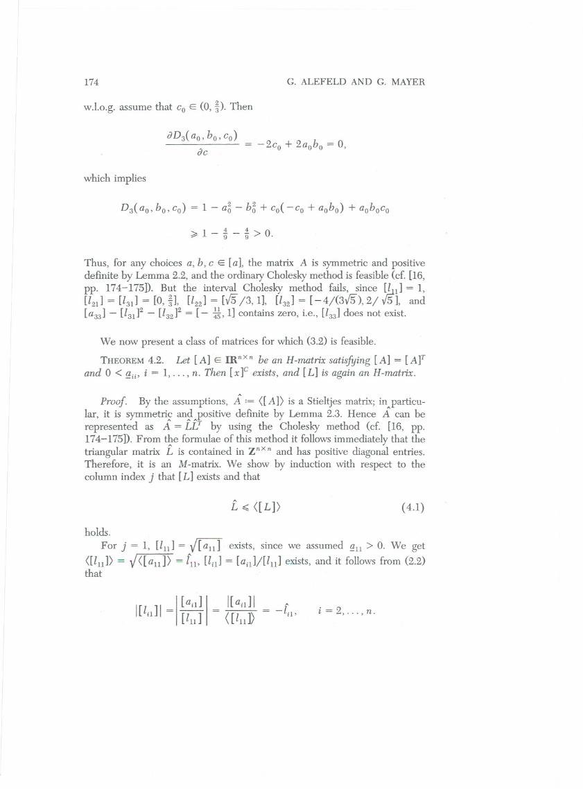
w.1.o.g. assume that Co E (0, ~). Then

JD3(ao,bo,co) = -2co+2aobo=0,Jc

which implies

D3(aO' bo, co) = 1 - a~ - b~ + co( -co + aobo) + aoboco

>-: 1 _1_1 >0:r 9 9 .

Thus, for any ehoices a, b, c E [a], the matrix A is symmetrie and positivedefinite by Lemma 2.2, and the ordinary Cholesky method is feasible (cf. [16,

pp. ~4-175E' B~t the in~erval Cholesky m~hod fails, sinee [ln] = 1,[121] - [131] - [0, 3], [122]- [VS/3,1], [132]- [-4/(3VS), 2/ '1/5], and[a33] - [131]2- [132]2= [- ~L 1] contains zero, i.e., [133]does not exist.

We now present a dass of matriees for whieh (3.2) is feasible.

THEOREM4.2. Let [A] E IRnXn be an H-rrw.trixsatisfying [A] = [A]Tand 0 < ~ii' i = 1,. . ., n. Then [xf exists, and [L] is again an H-rrw.trix.

Proof. Ey t.~e assumptions, A ;= ([ A]) isa Stieltjes matrix; in"particu-lar, it is symmetrie and positive definite by Lemma 2.3. Henee A ean berepresented as A = ii! by using the Cholesky method (cf. [16, pp.174-175]). From the formulae of this method it follows immediately that thetriangular matrix i is eontained in zn X n and has positive diagonal entries.Therefore, it is an M-matrix. We show by induetion with respect to thecolumn index j that [L] exists and that

i ~ ([L]) (4.1)

holds.

For j = 1, [Zu] = ~ exists, since we assumed ~u > O. We get

([lu]) = v'([au]) = Zu, [Zn] = [an]j[Zu] exists, and it follows from (2.2)that

I

[an]I

If an] 1 A

l[ln] I = [Zu] = /r1 1\ = -ln,i= 2,...,n.


Let all columns of [L] exist which have an index less than j > 1. Assurnethat (4.1) holds for all these columns, and deHne

j-I

[s] = [§, s] :=L (ljk]2k=I

and

[t] := [ajj] - [s].

Then using (2.2), {!:jj> 0, and the induction hypothesis we obtain

j-l j-l

0 < l] = < [ajj]) - L ~k < < [ajj]) - L I (ljd 12k=I k=l

(

j-I

)= {!:jj - s = t = <[t]) = [ajj] - L (ljk]2 .

k=I

Hence 0 $ [ajj] - Lt:1 [ljk]2. Therefore, [ljj] exists and satisfies ([ljj]) ~ l~j"For i > j we get

1 ( j-I \I [lij] I < Ir1 1\ \1[a;j]1 + L 1[l;dll[ljdIJ

Ik=I

1

(

j-I

)< f.. l[aij]1 + L ~k~k = -l~j')) k = I

This implies ~j < -I[lij]l.Thus, [xf exists, and the H-matrix property of[L] followsfrom Corollary

3.7.4in[13]. .

Note that an analogue ofTheorem 4.2 holds also for the interval Gaussianalgorithm, as was shown in [1].

COROLLARY4.3. Let [A] = [A]TE mnXn with 0 < {!:ii,i = 1,..., n.Then in .each of the following cases, [A] is an H -matrix and [x f exists.

(i) ([ A D is strictly diagonally dominant.(ii) < [ AD is irreducibly diagonally dominant.(iii) ([ A]) is regular and diagonally dominant.(iv) ([ A]) is positive definite.


Proof. By Theorem 2 in [10], [A] is an H-matrix in each of the fourcases; hence [x f existsbyTheorem4.2. .

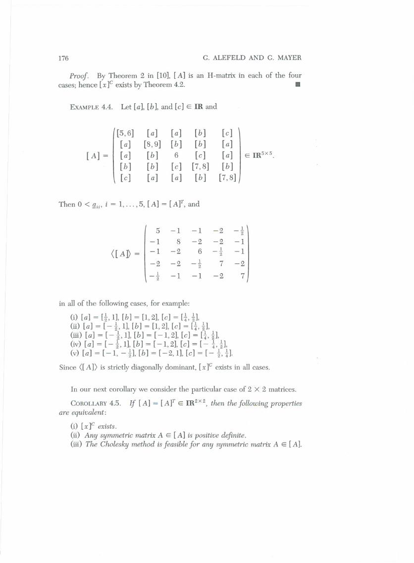
in all of the followingcases, for example:

(i) [a] = [t, 1], [b] = [1,2], [e] = [t i],(ü) [a] = [- i, 1], [b] = [1,2], [e] = [i, i],(iü) [a] = [-i,1], [b] = [-1,2], [e] = [ti],(iv) [a] = [- i, 1], [b] = [-1,2], [e] = [- t i],(v) [a] = [-1, -~], [b] = [-2,1], [e] = [- t,{c].

Since ([ A]) is strictly diagonally dominant, [x f exists in all cases.

In our next corollary we consider the particular case of 2 X 2 matrices.

COROLLARY4.5. 1f [A] = [A]TE m2X2, then thefollowing propertiesare equivalent:

(i) [x]C exists.

(ii) Any symmetrie matrix A E [A] is positive definite.(üi) The Cholesky method is feasible for any symmetrie matrix A E [A].

EXAMPLE4.4. Let [a], [b], and [e] E IR and

[5,6] [a] [a] [b] [e][a] [8,9] [b] [b] [a]

[A] = I [a] [b] 6 [e] [a] I E IRsxs.

[b] [b] [e] [7,8] [b]

[e] [a] [a] [b] [7,8]

Then 0 < {!ii' i = 1,...,5, [A] = [A]T, and

5 -1 -1 -2 1-2"

-1 8 -2 -2 -1

([ AD = I -1-2 6 1

-12

-2 -2 1 7 -221 -1 -1 -2 72


Proof. Ci) => (ii) follows from Lemma 2.2, sinee an = lfl > 0 and

det A = a22aU - a;2 =(

a22 - a;2)

. au = l~2lfl > O.au

(ii) => (iii) follows from Theorem 4.3.3 in [16].(iii) => Ci):Choose A E LA] sueh that A = AT and (A) = ([ A]) holds.

By the hypothesis, ln, l22 > 0; henee

au = lfl > 0,

2- 2 a12

a22 - l22 + - > O.an

This implies

([au]) = (au) = au > 0,

det([A]) = lanlla221-I[a12]12 = aUa22 - a;2 = l~2lfl > O.

Therefore, ([ A]) is symmetrie and positive definite, and f!n = an > 0,Q22 = a22 > O. The assertion follows from Corollary 4.3. a

COROLLARY4.6. If [A] E mnxn is an M-11UltriXsatisfying [A] = [A]T,then [x f exists.

As the example

A = (i ~)

illustrates, not every symmetrie H-matrix is an M-matrix. But symmetrieH-matriees are closely related to positive definite matriees, as the followingtheorem shows.

THEOREM 4.7. Let [A] E IRnXn be an H-11Ultrix satisfying [A] = [A]Tand 0 < Qii' i = 1, . . ., n. Then eaeh symmetrie 11UltriXA E [A] is positivedefinite.

Proof. Since ([ A]) is an M-matrix, (A) ~ ([ A]) is an M-matrix, too.Because Qii > 0, the matrix A has a nonnegative diagonal part D. Split A


into A = D - B. Then (A) = D -I BI = sI - (sI - D + IBI), s ER. Byaproperty whieh is equivalent to the definition of an M-matrix (ef. e.g. [5, (1.2)and (N38)], s ean be ehosen such that

s > p( sI - D + IBI) and sI - D + IBI ~ 0; (4.2)

henee sI ~ D, and

IsI - AI = IsI - D + BI ~ \sI - DI + IBI = sI - D + IBI

implies

p( sI - A) ~ p( sI - D + IBI) < s

by results in [17, §2.l], following from the Perron-Frobenius theorem.Therefore, all eigenvalues A of A satisfy Is - AI< s, whenee A > O. Thisprovesthe assertionbyLemma2.2. .

Note that the eonverse of Theorem 4.7 is not true. This is shown by thematrix of Example 4.1. Every symmetrie matrix A E [A] = [A]T is positivedefinite, and [A] satisfies f!:jj> 0, i = 1, . . . , n. But [A] is not an H-matrix,sinee othe:rwise, [x f would exist by Theorem 4.2.

The faet that the interval Cholesky faetorization need not exist for fuJinterval matrix whose symmetrie element matriees all are positive definite eanmake preeonditioning neeessary. An algorithm will be investigated in a futurepaper.

For tridiagonal matriees we have the following result.

THEOREM4.8. Let [A] = [A]T E IRnXn be a tridiagonal matrix, andlet i E [A] be any symmetrie matrix whieh satisfies (i) = ([ A]) andwhieh is positive definite. Then [A] is an H-matrix; in particular, allsymmetrie matriees A E [A] are positive definite, and [xf exists.

Proof. Sinee i is assumed to be positive definite, all diagonal entries ajjare positive. Therefore, (i) = ([ A]) and i E [A] implYf!:jj > 0, i =1, . .., n. By Lemma 2.4, i is an H-matrix; henee [A] is an H-matrix; too..Here we have used the equality (i) = ([ A]) onee more. The assertionfollows now from Theorems 4.2 and 4.7. .

COROLLARY4.9. Let [A] = [A]TE mnxn be a tridiagonalmatrix, andlet i E [A] be any symmetrie matrix whieh satisfies (i) = ([ A]). Ifi ean

CHüLESKY METHüD FüR INTERVAL DATA 179

be chosen such that it fulfills one of the three properties

Ci) Ä is totally positive,(ii) Ä is regular and totally nonnegative,(iii) Ä is oscillatory,

then [A] is an H-matrix; in particular, all symmetrie matriees A E [A] arepositive definite, and [x]C exists.

Praof. In the ease of (i), the leading prineipal minors are positive; heneeÄ is symmetrie positive definite, and Theorem 4.8 proves the assertion.

In the ease of (ii), the assumptions yield det A > O. Thus Lemma 2.2eombined with the inequality (116) in [8, p. 443] shows that the assumptionsof Theorem 4.8 hold. Therefore, the eorollary is proved in ease (ii).

Sinee det Äk > 0 for some integer k implies det Ä =1=0, (iii) is a partieu-lareaseof(ii). .

Example 4.1 and Theorems 4.2 and 4.7 show that [x]C does not neeessar-ily exist for interval matriees [A] = [A]T of whieh all symmetrie elementmatriees A are positive definite, but that for an important subclass of suehmatriees the existenee of [x]C is guaranteed.

We will now show that for an M-matrix [A] = [A]T the bounds of the

matrix [L] in step 1 of (3.2) ean be obtained independently of eaeh otherfrom the Cholesky deeomposition of the bounds ~, X

THEOREM 4.10. Let [A] = [A]T E mnxn be an M-matrix, and let

~ = L(l)(L(l))T, A = L(u)(L(u))T be the Cholesky decompositions of ~ and J\,respectively. Then L(l), L(u) are M-matriees. The matrix [L] fram the Choleskydecomposition of [A] can be represented as

[L] = [L(l), L(u)]; (4.3)

in particular, [L] is an M-matrix~

Proof. Sinee~, A are Stieltjes matriees, the formulae in (3.2) show atonee that L(l), L(u) E znxn. Theorem 4.2, applied to ~ and to J\, respee-tively, implies that they are M-matriees.

We now prove (4.3) by induetion with respect to the eolumn index j.For j = 1 we get at onee

[Zu] = ~ = [y'Qu,y'au] = [zW,ll~)]


and

[a' l]

[

a' l a' l

]

- ~ - =- ~ - (I) (u) .[Zn] -[I ] - 1(1)' l(u) - [ln ,ln], Z> 1,11 11 11

with l(u) ~ 0tl "" ,

where we have taken into account an < 0 for i > l.Assume now that (4.3) holds for all columns with an index less than j > l.

Then

pjj] ~ ([ ajj] - :$. [( lj,»)', (ljP)']r= [1(1) l('!)

])) , ))

and

(

}-1

) [

1 1

]

- - (u) (u) (I) (I) . - -[lij] - [aij] E [lik ljk ' lik ljk ] l('!)' 1(1)

k=l )) ))

= [1(1) I(U)]t) , t) for i > j,

since aij < 0 and l}';) < 0 for i > j. This proves the assertion. 11

We now consider the quality of the enclosure of [x f with respect to Ssymfrom (3.1).

THEOREM 4.11. Let [A] = [A]T E IRnXn be an M-matrix, and let

[b] E IRn satisfy Q ~ 0 or 0 E [b] or b < O. Then [xf = DSsym'

. Proof. Denote by (D(l)Y, (L(l»)S and (D(u»)S, (L(u»)S the matrices in the

r~resentation (3.7) when the interval Cholesky method is applied to .:1 andA, respectively. By Theorem 4.10 and by (3.5), these matrices are nonnega-tive, and

[D]" = [(D(U»)s,(D(I»)S], [L]" = [(L(U»)s,(L(l»)S].


Hence Theorem 3.4 proves

[ x]c =

[=1-ll?, X-q;]

[=1-ll?, =1-1b]

[X-ll?, =1-1b]

if b < 0,

if 0 E [b], .if l?> o.

COROLLARY4.12. Let [A] = [A]T E IRnXn be an M-matrix, and let

[b] E IRn satisfy l? > 0 or 0 E [b] or b < O. Then [x]C = OSsym = oS =[ X]G, where [x]G denotes the vector resulting from the interval Gaussianalgorithm applied to [A] and [b].

Proof. The proof follows at onee from Theorem 4.11 and from results in[4]. .

The authors thank an anonymous referee for his valuable comments whichimproved the paper.

REFERENCES

1 G. Alefeld, Über die Durchführbarkeit des Gaußschen Algorithmus bei Glei-chungen mit Intervallen als Koeffizienten, Comput. Suppl. 1:15-19 (1977).

2 G. A1efeld, On the c-onvergence of some interv'al-a..'it.~metic modifications ofNewton's method, SIAM J. Numer. Anal. 21:363-372 (1984).

3 G. Alefeld and J. Herzberger, Introduction to Interval Computations, Academic,New York, 1983.

4 W. Barth and E. Nuding, Optimale Lösung von Intervallgleichungssystemen,Computing 12:117-125 (1974).

5 A. Berman and R. J. Plemmons, Nonnegative Matrices in the MathematicalSciences, Academic, New York, 1979.

6 K. Fan, Topological proof for certain theorems on matrices with non-negativeelements, Monatsh. Math. 62:219-237 (1958).

7 A. Frommer, Lösung linearer Gleichungssysteme auf Parallelrechnern, Vieweg,Braunschweig, 1990.

8 F. S. Gantmacher, Matrizentheorie, Springer-Verlag, Berlin, 1986.9 D. J. Hartfiel, Conceming the solution set ofAx = b where P ,,;;;A ,,;;;Q and

p ,,;;;b ,,;;;q. Numer. Math. 35:355-359 (1980).10 G. Mayer, Old and new aspects for the interval Gaussian algorithm, in Computer

Arithmetic, Scientific Computation and Mathematical Modelling (E. Kaueher,S. M. Markov, and G. Mayer, Eds.), IMACS Ann. Comput. Appl. Math., Baltzer,Basel, 1991, pp. 329-349.

11 R. E. Moore, Interval Analysis, Prentiee-Hall, Englewood Cliffs, N.J., 1966.


12 A. Neumaier, New techniques for the analysis oflinear interval equations, LinearAlgebra Appl. 58:273-325 (1984).

13 A. Neumaier, Interval Methods for Systems of Equations, Cambridge V.P.,Cambridge, 1990.

14 K. Reichmann, Abbruch beim Intervall-Gauss-Algorithmus, Computing22:355-361 (1979).

15 H. Schwandt, Schnelle fast global konvergente Verfahren [ur die Fünf-Punkt-Diskretisierung der Poissongleichung mit Dirichletschen Randbedingungen aufRechteckgebieten, Dissertation, Techn. Vniv. Berlin, 1981.

16 J. Stoer and R. Bulirsch, Introduction to Numerical Analysis, Springer-Verlag,New York, 1980.

17 R. S. Varga, Matrix Iterative Analysis, Prentice-Hall, Englewood Cliffs, N.}.,1963.

Received 12 October 1992; final manuscript accepted 25 November 1992

Documents

D-76128 Karlsruhe, Germany - KITna.math.kit.edu/alefeld/download/1993_The_Cholesky_method_for... · , D-76128 Karlsruhe, Germany ... analysis and matrix theory (Section 2), ... LINEAR