Data Analysis and Statistical Methods Statistics 651

Data Analysis and Statistical MethodsStatistics 651

http://www.stat.tamu.edu/~suhasini/teaching.html

Lecture 20 (MWF) The Wilcoxon Sum Rank test (Mann-Whitney test)

Suhasini Subba Rao

Lecture 20(MWF) Review of independent sample t-test and the Wilcoxon sum rank test (in the case of small samples and outliers)

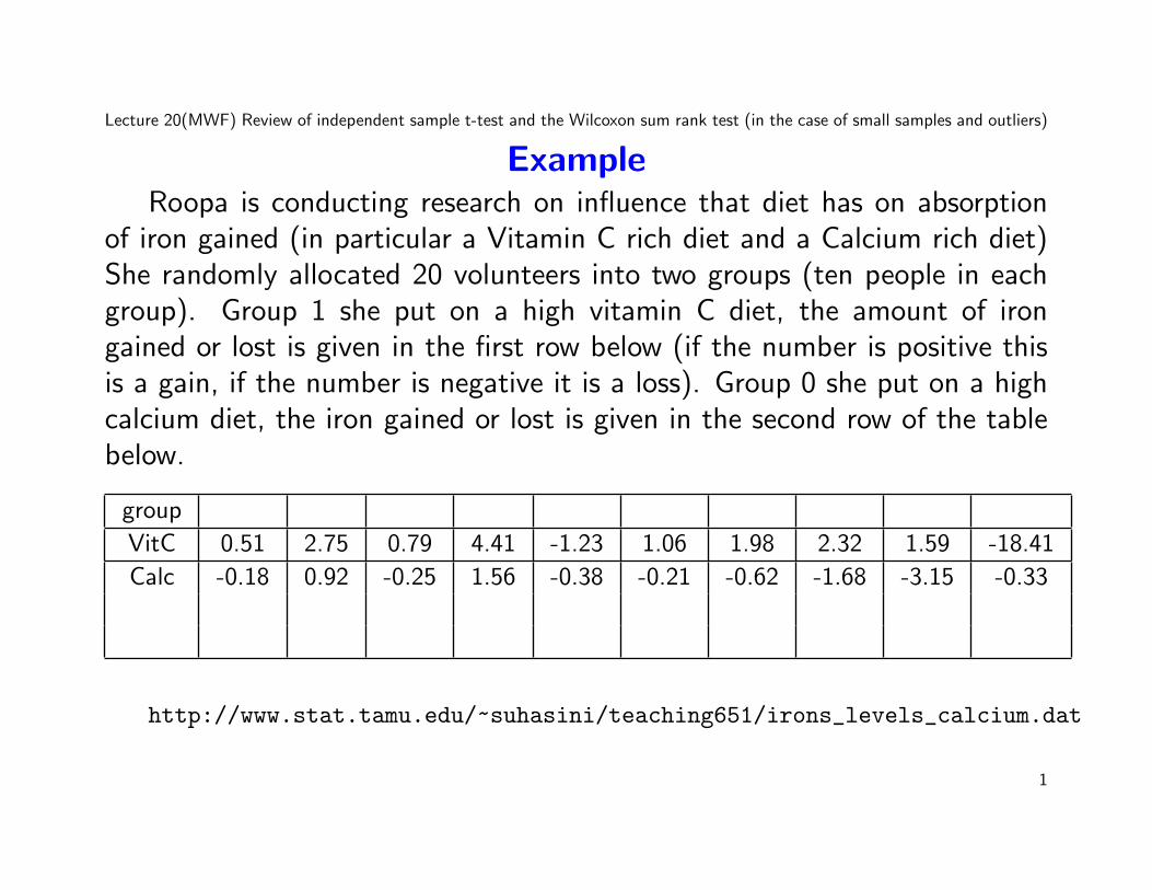
ExampleRoopa is conducting research on influence that diet has on absorption

of iron gained (in particular a Vitamin C rich diet and a Calcium rich diet)She randomly allocated 20 volunteers into two groups (ten people in eachgroup). Group 1 she put on a high vitamin C diet, the amount of irongained or lost is given in the first row below (if the number is positive thisis a gain, if the number is negative it is a loss). Group 0 she put on a highcalcium diet, the iron gained or lost is given in the second row of the tablebelow.

group

VitC 0.51 2.75 0.79 4.41 -1.23 1.06 1.98 2.32 1.59 -18.41

Calc -0.18 0.92 -0.25 1.56 -0.38 -0.21 -0.62 -1.68 -3.15 -0.33

http://www.stat.tamu.edu/~suhasini/teaching651/irons_levels_calcium.dat

1


She wants to investigate whether the mean absorption of iron of peopleon a high Vitamin C is more than the absorption of those on high calcium.

2


SolutionRoopa’s research hypothesis is that the average amount of iron absorbed

is higher for vitamin rich diets. Let µV itC denote the mean amount of irongained on the vitamin C diet and µCalc denote the mean amount of irongained on the high calcium diet. Roopa’s null and alternative hypothesesare H0 : µV itC − µCalc ≤ 0 against HA : µV itC − µCalc > 0.

3


Result of Roopa’s t-test

• From the output using the one-sided test we see that the p-value is48.65%, this p-value is a lot larger than the 5% significance level. hencewe cannot reject the null. Why the negative result?

– May be a small sample size to detect a difference even if there is one?– There is no difference between absorption of iron when a person takes

either calcium of vitamin C.

• Aside Negative results can also be of academic interest see the interestingarticle

w.economist.com/news/leaders/21588069-scientific-research-has-changed-world-now-it-needs-change-itself-how-science-goes-wrong, one aspect ofthis argument is that negative results need to be published.

4


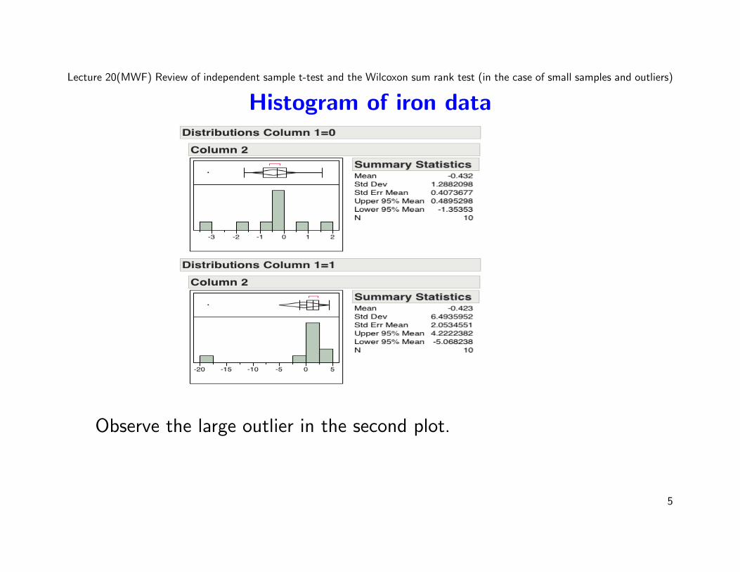
Histogram of iron data

Observe the large outlier in the second plot.

5


• Besides the sample size, there can be two reasons that we may not beunable to reject the null, even if the alternative is true. Both thesereasons are related to the outlier −18.41 we see in the plot.

– This outlier makes a difference. It pulls down the sample mean for theiron level in Diet 0.

– The large outlier also makes the sample standard deviation very large.

• Both these factors contribute to our being less likely to reject the null (bymaking the difference in the sample means smaller and the non-rejectionregions wider).

• The above data set illustrates why we may, in certain cases, want to usea test which is more robust to outliers. The outlier carries too muchweight, and is too influential.

6


• In this example, the outlier was was making the sample means closer.

• In other examples, one outlier can make the difference appear greaterand give the appearance of a difference.

• When outliers exist do not remove them!

• Instead we use tests that gives less weight to individual outliers.

One solution is to use ranks rather than raw observations.

7


When it is best not to use the independent t-test

• In the case that n or m is small and has several outliers or appearsskewed (non-symmetric) the t-test may give unreliable results:

– Outliers can wrongly shift the sample mean to high or low, makinga comparison difficult, they can also make the standard errors largerthan what they should be.

– If the observations come from a distribution which is skewed, and thesample size is not sufficiently large. Then the central limit theoremmay not hold, in which case the t-test is inappropropiate.

– In a nutshell, the assumption that the difference in the sample meansis normally distributed may not hold (the original data set is toonon-normal for the central limit theorem to have kicked in).

8


A second look at the iron data

There appears to be a ‘separation’ in the two data, that could be difficultto explain by random chance (ie, if both data sets came from the samedistribution how likely can be get a sample that looks this separated?). Howto quantify this separation?

9


The Wilcoxon Rank sum test/ Mann-Whitney U statistic

In the hypothesis test we do notassume normality, but we do requirethe two distributions are the sameexcept for a possible shift. In otherwords both distributions have thesame “shape”.

• We do not characterise the hypothesis test in terms of the mean. Insteadwe do the characterisation in terms of the ’location’ of the distribution.

– H0: The populations have identical distributions.– HA: One population is a shift of the other (as in the plot above).

• The independence assumption still holds.

10


• The test is often called ‘distribution free’ (or nonparametric) meaningthat it does not require any assumptions on the distribution of theobservations.

11


Ranking Data

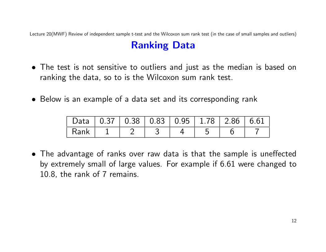
• The test is not sensitive to outliers and just as the median is based onranking the data, so to is the Wilcoxon sum rank test.

• Below is an example of a data set and its corresponding rank

Data 0.37 0.38 0.83 0.95 1.78 2.86 6.61Rank 1 2 3 4 5 6 7

• The advantage of ranks over raw data is that the sample is uneffectedby extremely small of large values. For example if 6.61 were changed to10.8, the rank of 7 remains.

12


Back to the Iron vs Vitamin C data set

The Wilcoxon test is based on collectively ranking the data.

13


• We count the total ranks in each group. And we use the “rank sums” asthe basis of the test.

• Effectively, if both groups are drawn from the same population and thesample sizes in both groups are the same we would expect the rank sumsto be about the same too.

• As it is difficult to clearly rank the above data set. We start with asimpler example. And return to this data set later.

14


The Wilcoxon Rank sum test: exampleIn a study, 19 mold sensitive volunteers were exposed to mold. The

objective of the study was to understand the influence antihistamines hadon the allergic reaction to the mold. The 19 volunteers were placed intotwo treament groups, one of size 10 the other of size 9. Group 1 (size 10)was given the antihistamine, Group 2 (size 9) was given the placebo. Thesize of the allergic reaction is given below.

Antihistimine 0.90 0.37 1.63 0.15 0.95 0.78 0.05 0.61 0.51 0.20

Placebo 1.60 1.50 1.76 1.44 1.11 3.07 1.05 1.27 2.56

• Data:

http://www.stat.tamu.edu/~suhasini/teaching651/antihistamine_placebo.

dat.

• Our aim is to see whether in general people with dust allergies have

15


smaller reaction when taking an antihistamine than those on a control(placebo). Our hypotheses are:

H0: distribution of both the antihistamine and placebo populations arethe same or antihistamine is a right shift of the placebo (view this asH0 : µA ≥ µP ).

HA: distribution of the antihistamine is a left shift of the placebo (viewthis as HA : µA < µP ).

16


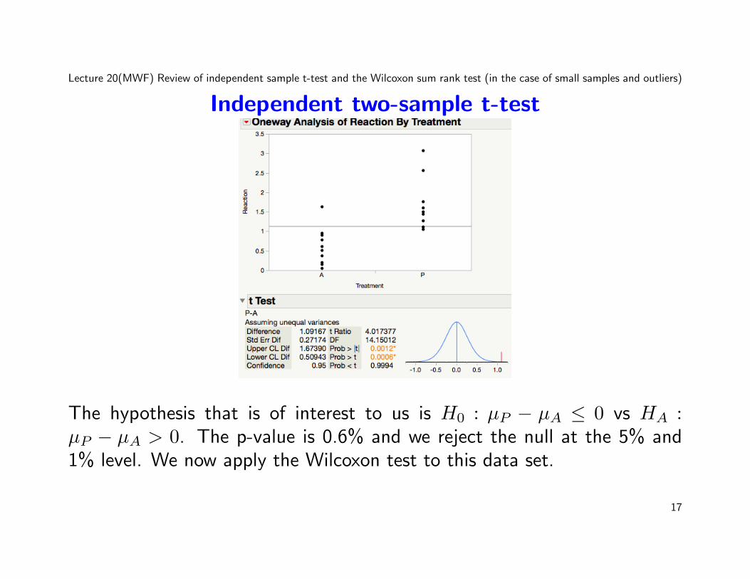
Independent two-sample t-test

The hypothesis that is of interest to us is H0 : µP − µA ≤ 0 vs HA :µP − µA > 0. The p-value is 0.6% and we reject the null at the 5% and1% level. We now apply the Wilcoxon test to this data set.

17


Distribution under null and alternative

18


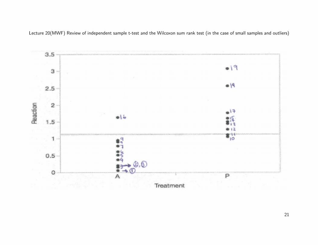
Dotplot of the data

Data plotted side by side. Visually there appears to be a right shift ofthe placebo group. Is this for real (something systematic in the population)?How likely is such a shift in data when really both the placebo and theantihistamine data came from the same distribution?

19


Basic idea of a Wilcoxon Rank sum test

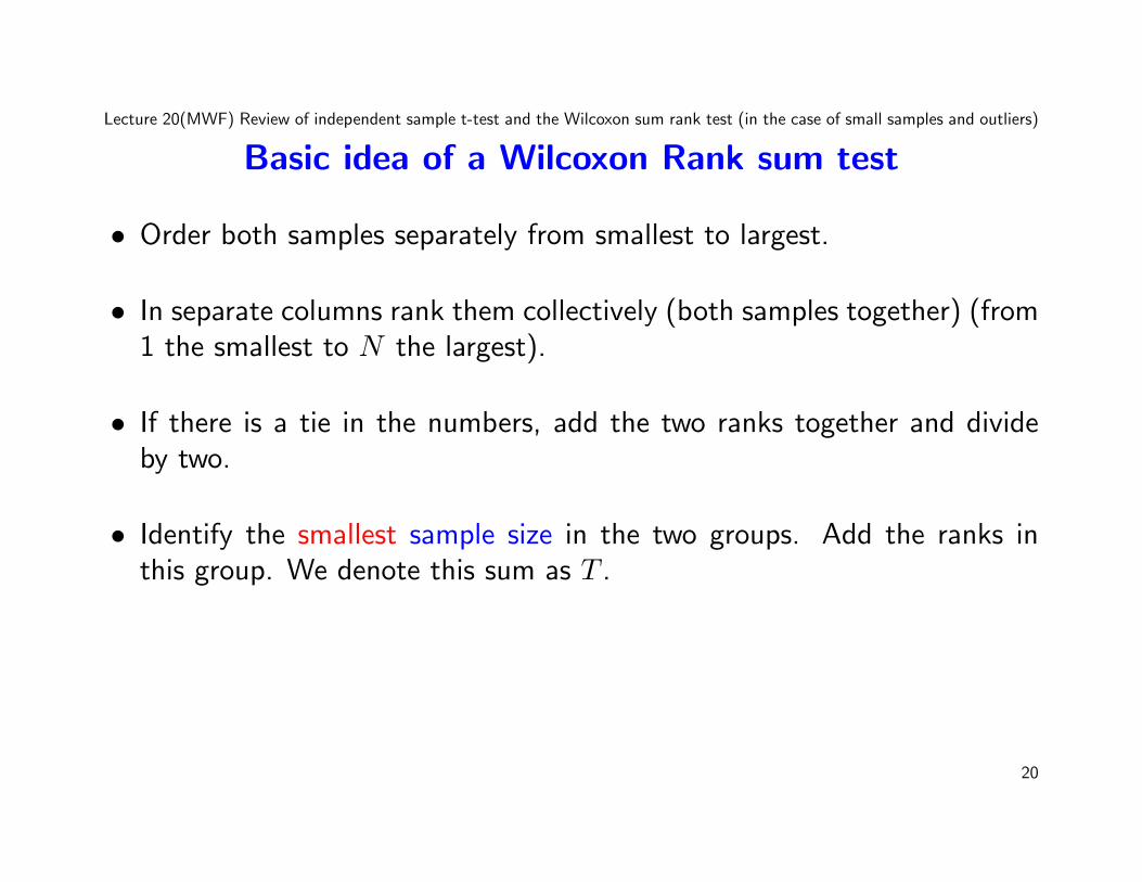
• Order both samples separately from smallest to largest.

• In separate columns rank them collectively (both samples together) (from1 the smallest to N the largest).

• If there is a tie in the numbers, add the two ranks together and divideby two.

• Identify the smallest sample size in the two groups. Add the ranks inthis group. We denote this sum as T .

20


21


Example

Antihistamine Rank Control/Placebo Rank

0.05 1 1.05 10

0.15 2 1.11 11

0.20 3 1.27 12

0.37 4 1.44 13

0.51 5 1.50 14

0.61 6 1.60 15

0.78 7 1.76 17

0.90 8 2.56 18

0.95 9 3.07 19

1.63 16

T 61 129

22


Interpreting T

• The total sum of all the ranks is 19× 20/2 = 190. This is a non-randomquantity that only depends on the sample size.

• These following quantities are important.

The ranks corresponding to the smallest sample size is T = 129.Convention means we always focus on the rank corresponding to thesmallest sample size.

The ranks corresponding to the larger sample size is T = 61.

• The sum of ranks from the smallest sample size is T = 129 is randomand depends on the the outcomes from the two groups.

Compare T = 129 with the sum of the larger sample size 61. 129 issubstantially larger than 61.

23


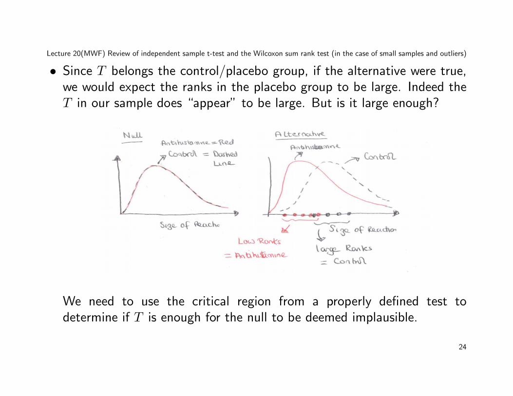
• Since T belongs the control/placebo group, if the alternative were true,we would expect the ranks in the placebo group to be large. Indeed theT in our sample does “appear” to be large. But is it large enough?

We need to use the critical region from a properly defined test todetermine if T is enough for the null to be deemed implausible.

24


25


Critical region: One-sided test 5% pointing RIGHT

• Use α = 0.05 and one-sided. Too prove the alternative at the 5% levelwe have to determine if T (which corresponds to the placebo group) istoo large for the null to be plausible.

• Choose n1 = 9 and n2 = 10 (it does not matter which way round youchoose 9 and 10) and find where they cross. Since we are conductinga one-sided test to determine if T is too large, use the largest value in[69, 111] as the critical point.

• The critical region for the one-sided test is any value greater than 111.

• T = 129 > 111, therefore we reject the null and determine that using aantihistamine reduces the area of reaction (at the 5% level).

26


Critical region: One-sided test 5% pointing LEFT

• If there is reason to believe that Antihistamines may increase the size ofthe reaction. Then we should use the following one-sided test:

H0 : Placebo and Antihistamines have the same distribution or theplacebo distribution is to left of the antihistamine distribution.

HA : The distribution of antihistamine population is to the right ofplacebo population. Or equivalently the distribution of the placebo is toleft of the antihistamine group. Draw the plot:

27


• We use the same T = 129, but reject the null if it is too small.

• The critical region is any number less than 69 (using n1 = 10 andn2 = 9). Since T = 129 > 69 we cannot reject then null.

28


Critical region: Two-sided test 5% level

• If we want to test

H0 : Placebo and Antihistamines have the same distribution.

HA : The distribution of antihistamine population is a shift of the placebopopulation.

• Look up the Table 5, using the 5% level, two-sided test. The intersectionof n1 = 10 and n2 = 9 gives the non-rejection region [66, 114].

If T lies outside this region we reject the null.

• Since T = 129 is not inside [66, 114] we reject the null in the two-sidedtest and determine there is a difference. Which makes sense, if we rejectthe null in a one-sided test than we have to reject the null for a two-sidedtest.

29


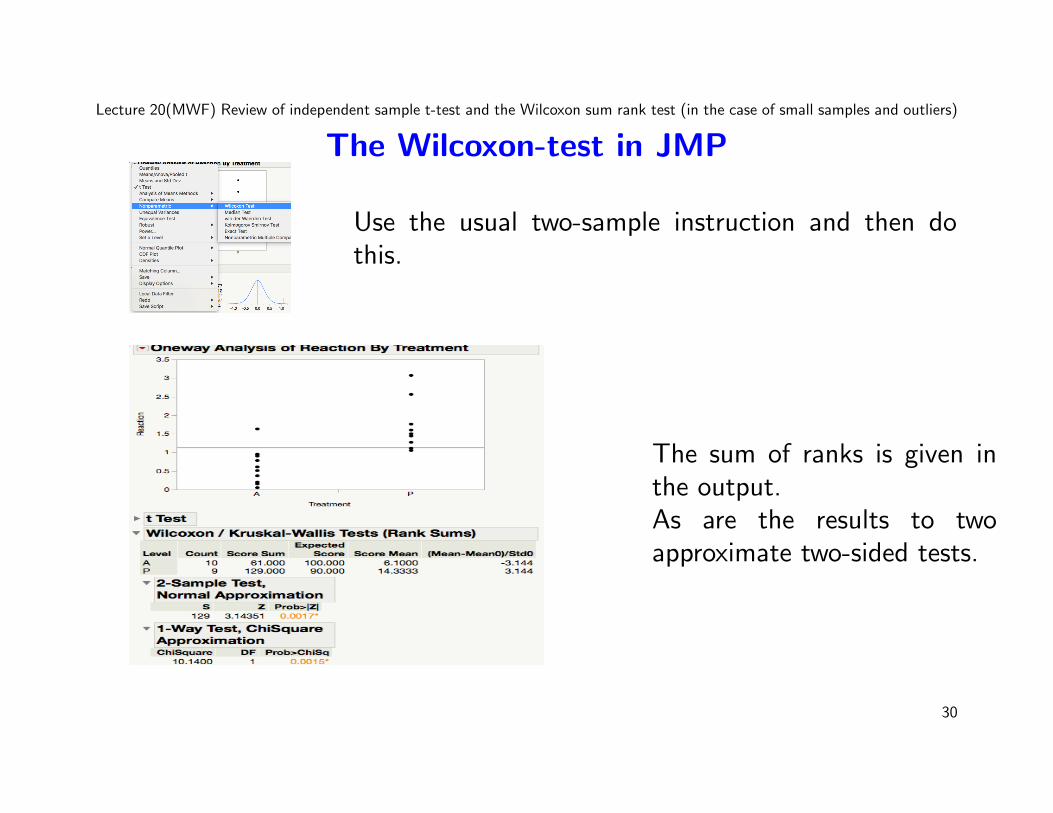
The Wilcoxon-test in JMP

Use the usual two-sample instruction and then dothis.

The sum of ranks is given inthe output.As are the results to twoapproximate two-sided tests.

30


Discussion of JMP output

• The JMP output gives the sum of the ranks; 129 for the small samplesize and 61 for the large sample size.

• It also gives p-values, however, these are calculated using certaindistributional approximations.

Whereas the Wilcoxon tables give the exact critical regions.

• If the sample sizes are less than 10, use the Wilcoxon tables.

31


Example 2: Iron data using the Wilcoxon Rank testgroup

VitC 0.51 2.75 0.79 4.41 -1.23 1.06 1.98 2.32 1.59 -18.41

Calc -0.18 0.92 -0.25 1.56 -0.38 -0.21 -0.62 -1.68 -3.15 -0.33

• H0 : Vit C and Calcium have the same distribution or the Vit distributionis to left of the Calcium distribution. HA : The distribution of VitaminC population is to the right of Calcium population. Draw plot:

32


• The sample sizes for both groups is n1 = 10 and n2 = 10. This meanswe can pick any sample size for analysis.

• We pick the the ranks corresponding to the vitamin C group.

The choice is arbitrary. However, under the alternative we are seeking todetermine if the vitamin C ranks are “too large” for the null to hold.

33


Example 2: Iron data using the Wilcoxon Rank test

34


Example 2: cont• From the JMP output the rank corresponding to the Vitamin C group is

132.

• Looking at the alternative we reject the null if T = 132 is larger thanwhat we expect under the null.

• We do the one-sided test at the 5% level n1 = 10 and n2 = 10 gives83, 127. Since we want to determine if T is too large. The critical regionis any number larger than 127.

• Since T = 132 > 127 we reject the null at the 5% level.

• There is some evidence in the data to suggest that those who consumevitamin C with tend to increase iron absorption over those who consumeCalcium with Iron.

35


Example 3: Diet example using Wilcoxon Sum Rank test

Recall the sample in the diet data is rather small.

Diet I 2.9 2.7 3.9 2.7 2.1 2.6 2.2 4.2 5.0 0.7Diet II 3.5 2.5 3.8 8.1 3.6 2.5 5.0 2.9 2.3 3

• Test the hypothesis that the two diets are the same against the alternativethat the two diets are different.

• Test the hypothesis that the two diets are the same against the alternativethat diet II is better than diet I.

36


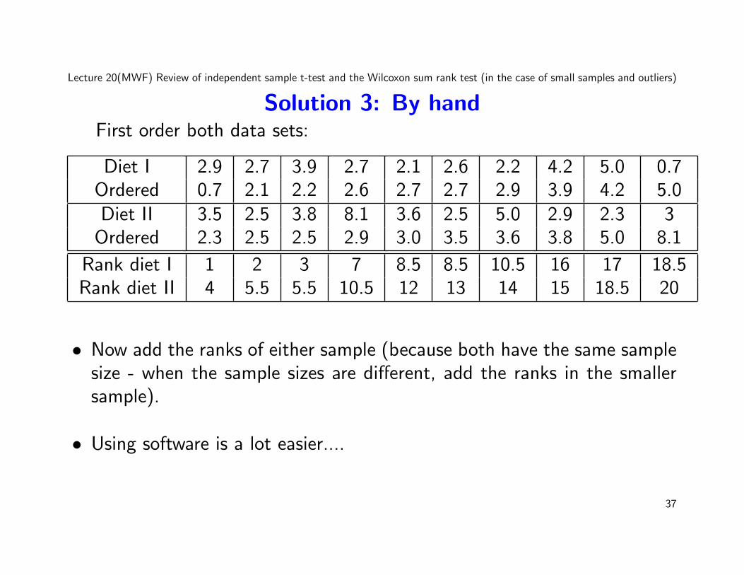
Solution 3: By handFirst order both data sets:

Diet I 2.9 2.7 3.9 2.7 2.1 2.6 2.2 4.2 5.0 0.7Ordered 0.7 2.1 2.2 2.6 2.7 2.7 2.9 3.9 4.2 5.0Diet II 3.5 2.5 3.8 8.1 3.6 2.5 5.0 2.9 2.3 3

Ordered 2.3 2.5 2.5 2.9 3.0 3.5 3.6 3.8 5.0 8.1

Rank diet I 1 2 3 7 8.5 8.5 10.5 16 17 18.5Rank diet II 4 5.5 5.5 10.5 12 13 14 15 18.5 20

• Now add the ranks of either sample (because both have the same samplesize - when the sample sizes are different, add the ranks in the smallersample).

• Using software is a lot easier....

37


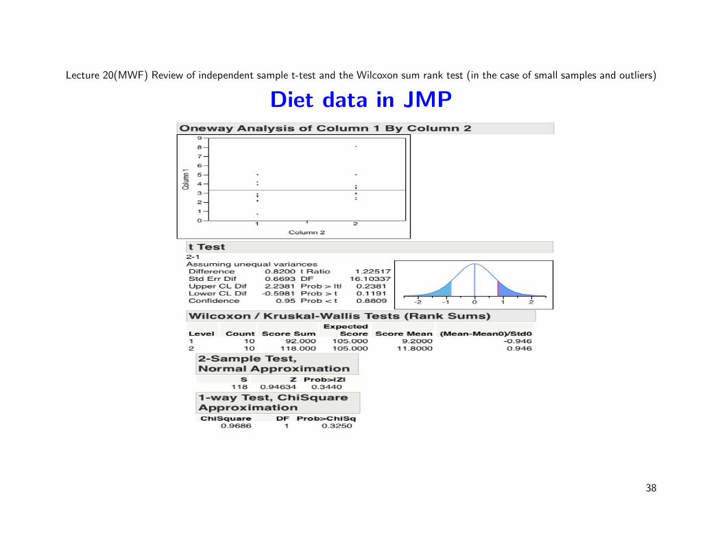
Diet data in JMP

38


Determining the rejection region

• The sum of the ranks in Diet I is T = 92. The sum of ranks of Diet II isT = 118 (we can use either sums since the sample sizes of both samplesare the same).

• We use these numbers to do the formal test.

Testing: H0 : The distributions of both populations are both the same.HA : One distribution is a shift of another (two sided test).

• Kook up Table 5, the first table (the column n2 = 10 and n1 = 10).

• Reading the table we see that the non-rejection region is

[79, 131].

39


• Since T = 118 lies in [79, 131] there is not enough evidence to reject H0

(noting if T were to lie outside this region there is enough evidence toreject H0). T = 118 is neither too small or too big to suggest the nullis implausible.

40


Warnings

• Nonparametric tests are conservative, meaning that even if the alternativeis true, the test errs on the cautious side and tends not to reject the null(see the example on the next slide).

• We cannot test more complex hypothesis such as H0 : µY − µX ≤ 0.3vs HA : µY − µX > 0.3 using a nonparametric test.

• We cannot make confidence intervals with nonparametric.

• One underlying assumption is that the shape of the distributions forpopulations is the same, we are only testing shifts of the distributions.

• If the shapes of the two populations are different, such as one distributionbeing narrower than another the test can yield incorrect results. This is

41


not an issue for the independent two sample t-test. The main assumptionthere is that the sample means are close to normal.

42


Why the Wilcoxon sum rank test is called conservative

• Observe that there are three observations in each of the two groups.

• There appears to be a clear difference between the two groups.

43


• There is a large separating between the two groups and the separationbetween the groups is greater than the variation/spread within thegroups.

• Result of Independent sample t-test Despite the sample sizes beingextremely small, the t-test test detects a difference and the p-value isextremely small (less than 0.02%). Hence there is evidence to suggestthat this data has been take from two populations with two differentmeans.

• Results of the Wilcoxon sum rank test The sum of the ranks is 6 or 15(as the sample size in both groups is the same it does not matter whichrank is chosen). The non-rejection region (for the two sided test) is[5, 16]. Since 6 (or 15) is within this region, we cannot reject the nullusing the Wilcoxon test at the 5% level. The p-value for this test is 5%of greater.

44


• The reason for the large discrepency between the p-values of theindependent sample t-test and the Wilcoxon test is that Wilcoxon testdoes not take into account the magntitude difference between groupA and B.

• One the other hand the independent sample t-test does account for thedifference in magnitudes and spread.

• To illustrate this, consider the new data set on the next slide. Thedifference between the groups is less (and the spread greater).

• This leads to a larger p-value for the independent sample t-test.

• But for the Wilcoxon sum-rank test the ranks are identical.

45


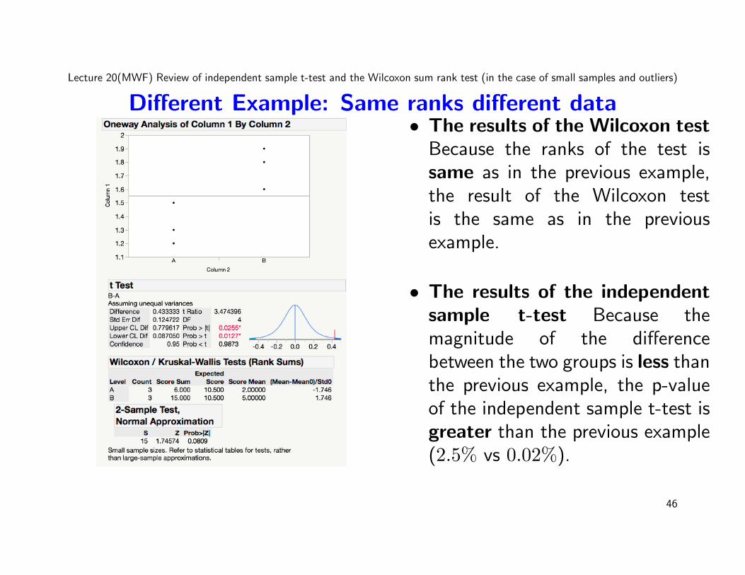
Different Example: Same ranks different data• The results of the Wilcoxon test

Because the ranks of the test issame as in the previous example,the result of the Wilcoxon testis the same as in the previousexample.

• The results of the independentsample t-test Because themagnitude of the differencebetween the two groups is less thanthe previous example, the p-valueof the independent sample t-test isgreater than the previous example(2.5% vs 0.02%).

46

Documents

Data Analysis and Statistical Methods Statistics 651