Data Analysis for Effluent Limitations using Monte Carlo · use of the Monte Carlo method must be justified through prior assessment of limit requirements using simpler methods. Implementing

i

Association of Idaho Cities

3100 South Vista, Suite 201, Boise, Idaho 83705 Telephone (208) 344-8594 Fax (208) 344-8677 www.idahocities.org

10/8/2019

Data Analysis for Effluent Limitations using Monte Carlo

http://www.idahocities.org/

i

Special Thanks & Acknowledgements The Association of Idaho Cities would like to thank HDR staff Michael Kasch, Allison Tyner

Hornak, Tom Dupuis, and Dave Clark; Boise City staff Kate Harris; Idaho Department of

Environmental Quality staff Mary Anne Nelson, Troy Smith, A.J. Maupin, and Matt Stutzman.

ii

Table of Contents Special Thanks & Acknowledgements ............................................................................................. i

Table of Contents .............................................................................................................................ii

List of Tables ................................................................................................................................... iv

List of Figures ................................................................................................................................... v

Abbreviations and Acronyms .......................................................................................................... vi

Introduction .................................................................................................................................... 1

The Idaho Reasonable Potential Analysis Workbook ................................................................. 1

SECTION 1: Monte Carlo – Getting Started .................................................................................... 3

Monte Carlo – RPTE and Effluent Limits ..................................................................................... 3

Monte Carlo – Data Requirements ............................................................................................. 4

Monte Carlo – Software Options ................................................................................................ 6

SECTION 2: Monte Carlo - General Process .................................................................................... 7

Step 1: Data Compilation ............................................................................................................ 8

Step 2: Representative Data and Distributions ......................................................................... 10

Step 3: RPTE – Using RPA Workbook ........................................................................................ 11

Step 4: RPTE – Using Monte Carlo: The Mixing Equation ......................................................... 12

Step 5: RPTE – Using Monte Carlo: The Result Variable ........................................................... 14

Step 6: RPTE – Using Monte Carlo ............................................................................................ 16

Step 7: Effluent Limits – Using RPA Workbook ......................................................................... 17

Step 8: Effluent Limits – Using Monte Carlo ............................................................................. 17

Step 9: Effluent Limits – RPA Workbook versus Monte Carlo .................................................. 18

SECTION 3: Monte Carlo – Illustrative Examples .......................................................................... 19

Monte Carlo Example – Facility P .............................................................................................. 19

Facility P - Data Compilation .................................................................................................. 19

Facility P – RPTE Using RPA Workbook .................................................................................. 21

Facility P – RPTE Using Monte Carlo ...................................................................................... 22

Facility P – Effluent Limits Using RPA Workbook .................................................................. 23

Facility P - Effluent Limits Using Monte Carlo ....................................................................... 24

Facility P - Effluent Limits RPA Workbook versus Monte Carlo ............................................. 26

Monte Carlo Example – Facility C .............................................................................................. 28

iii

Facility C - Data Compilation ................................................................................................. 28

Facility C – RPTE Using RPA Workbook.................................................................................. 30

Facility C - RPTE Using Monte Carlo ...................................................................................... 32

Facility C - Effluent Limits Using RPA Workbook ................................................................... 33

Facility C - Effluent Limits Using Monte Carlo ....................................................................... 33

Facility C - Effluent Limits RPA Workbook versus Monte Carlo ............................................ 35

Monte Carlo Example – Facility M ............................................................................................ 37

Facility M - Data Compilation ................................................................................................ 37

Facility M – RPTE Using RPA Workbook ................................................................................ 39

Facility M - RPTE Using Monte Carlo ..................................................................................... 41

Facility M - Effluent Limits Using RPA Workbook .................................................................. 42

Facility M - Effluent Limits Using Monte Carlo ...................................................................... 43

Facility M - Effluent Limits RPA Workbook versus Monte Carlo ........................................... 44

Monte Carlo Example – Facility B .............................................................................................. 46

Facility B - Data Compilation ................................................................................................. 46

Facility B – RPTE Using RPA Workbook ................................................................................. 48

Facility B - RPTE Using Monte Carlo ...................................................................................... 49

Facility B - Effluent Limits Using RPA Workbook ................................................................... 51

Facility B - Effluent Limits Using Monte Carlo ....................................................................... 52

Facility B - Effluent Limits RPA Workbook versus Monte Carlo ............................................ 53

References and Resources ............................................................................................................ 55

iv

List of Tables Table 1: Examples of Software Options for Monte Carlo ................................................................ 6

Table 2: Receiving Body River Flow Statistics .................................................................................. 9

Table 3. Receiving Body River Characteristics ................................................................................. 9

Table 4. Facility Effluent Characteristics ........................................................................................ 10

Table 5. River Q USGS Flow Gage Statistics ................................................................................... 19

Table 6. River Q Characteristics ..................................................................................................... 20

Table 7. Facility P Characteristics .................................................................................................. 21

Table 8. Facility P RPTE results using Monte Carlo ........................................................................ 23

Table 9. Comparison of Potential Effluent Limitations .................................................................. 27

Table 10. River S USGS Flow Gage Statistics .................................................................................. 28

Table 11. River S Characteristics .................................................................................................... 29

Table 12. Facility C Characteristics ................................................................................................ 30

Table 13. Facility C RPTE results using Monte Carlo ...................................................................... 32

Table 14. Comparison of Potential Effluent Limitations ................................................................ 36

Table 15. River F USGS Flow Gage Statistics .................................................................................. 37

Table 16. River F Characteristics.................................................................................................... 38

Table 17. Facility M Characteristics ............................................................................................... 39

Table 18. Facility M RPTE results using Monte Carlo..................................................................... 41


Table 20. River B USGS Flow Gage Statistics ................................................................................. 46

Table 21. River B Characteristics ................................................................................................... 47

Table 22. Facility B Characteristics ................................................................................................ 48

Table 23. Facility B RPTE results using Monte Carlo ...................................................................... 50


v

List of Figures Figure 1. P-P Plot for a lognormal distribution .............................................................................. 11

Figure 2. Example of RPA Workbook with an Example Facility RPTE for a Pollutant of Concern .. 12

Figure 3. Defining a distribution for Monte Carlo in XLSTAT ......................................................... 14

Figure 4. Defining a result variable for Monte Carlo in XLSTAT ..................................................... 14

Figure 5. Running a Monte Carlo in XLSTAT .................................................................................. 15

Figure 6. Monte Carlo simulation results ...................................................................................... 16

Figure 7. Example of RPA Workbook with an Example Facility Effluent Limits for a Pollutant of

Concern ......................................................................................................................................... 17

Figure 8. Facility P RPTE Results from RPA Workbook ................................................................... 22

Figure 9. Facility P Effluent Limits from RPA Workbook ................................................................ 24

Figure 10. Results of a Range of Effluent Concentrations from Monte Carlo, Ammonia .............. 25

Figure 11. Results of a Range of Effluent Concentrations from Monte Carlo, Zinc ....................... 26

Figure 12. Facility C RPTE Results from RPA Workbook ................................................................ 31

Figure 13. Facility C Effluent Limits from RPA Workbook .............................................................. 33



Figure 16. Facility M RPTE Results from RPA Workbook ............................................................... 40

Figure 17. Facility M Effluent Limits from RPA Workbook ............................................................. 42



Figure 20. Facility B RPTE Results from RPA Workbook ................................................................ 49

Figure 21. Facility B Effluent Limits from RPA Workbook .............................................................. 51



vi

Abbreviations and Acronyms μ microgram

AIC Association of Idaho Cities

AML average monthly limit

CCC criterion continuous concentration

cfs cubic feet per second

CMC criterion maximum concentration

CV coefficient of variation

DEQ Idaho Department of Environmental Quality

ELDG IPDES Effluent Limit Development Guidance

EPA United States Environmental Protection Agency

IPDES Idaho Pollutant Discharge Elimination System

LTA long-term average

MDL maximum daily limit

POTW publicly owned treatment works

RPA reasonable potential analysis

RPTE reasonable potential to exceed

WQBEL water quality-based effluent limit

1

Introduction The Association of Idaho Cities (AIC) is providing this guidance on the application of Monte

Carlo to develop water quality-based effluent limits (WQBELs) for the benefit of our members

with publicly owned treatment works (POTWs). An analysis of potential WQBELs may include

Monte Carlo when data are available and when limits needing to reflect the receiving water’s

load carrying capacity are preferred. However, Monte Carlo does not guarantee different

effluent limits, and may provide either less or more stringent treatment requirements to meet

water quality criteria within the receiving water body.

The Idaho Department of Environmental Quality (DEQ) lists the use of Monte Carlo as an

example of a probabilistic approach in the development of a Reasonable Potential Analysis

(RPA, DEQ 2017). AIC encourages those wishing to apply Monte Carlo work closely with their

DEQ permit writer for a common understanding and to ensure the regulatory support

necessary for a successful outcome.

The historical use of Monte Carlo for assessing effluent limits (i.e., permissible discharges) is not

well documented. The use may only be documented in individual permit fact sheets. Not only

are these information sources difficult to locate, but they are also not permanent and may be

lost during the renewal of the permit. Implementing the Monte Carlo method to develop

receiving water appropriate limits should only occur after other methods have indicated that

site conditions warrant this detailed analysis.

It is highly recommended to discuss a possible Monte Carlo analysis with DEQ prior to initiating

this analysis. There are data quality objectives, quality assurance and control concerns, and

general “appropriateness” issues to discuss and agree upon prior to a POTW expending their

limited resources on an effort the DEQ cannot support. For example, many receiving water

bodies in Idaho have established TMDLs with waste load allocations for POTWs. In these cases,

and for these parameters, there is no assimilative capacity to allow adjustments to the

WQBELs.

The Idaho Reasonable Potential Analysis Workbook DEQ’s Idaho Pollutant Discharge Elimination System (IPDES) Program has developed Effluent

Limit Development Guidance (ELDG) and an associated Reasonable Potential Analysis (RPA)

workbook1 to help DEQ personnel, the regulated community, and public users understand and

evaluate whether there is a reasonable potential to exceed (RPTE) water quality standards

within a receiving water body due to effluent discharges.

The RPA Workbook is a method to develop WQBELs and associated effluent limits when limited

data are available. EPA Region 10 developed the RPA Workbook to evaluate the need for

WQBELs and to calculate effluent limits based on EPA’s Technical Support Document for Water

1 https://www.deq.idaho.gov/media/60181412/ipdes-tsd-rpa-workbook.xlsx

https://www.deq.idaho.gov/media/60181412/ipdes-tsd-rpa-workbook.xlsx

2

Quality-based Toxics Control. DEQ has customized the RPA workbook to implement Idaho

specific water quality requirements.

It is recommended that Monte Carlo be used in a tiered approach to assess permit limits. The

use of the Monte Carlo method must be justified through prior assessment of limit

requirements using simpler methods. Implementing the Monte Carlo method when it is not

justified may prove to be expensive and not yield results that are any more appropriate than

simpler methods of analysis.

3

SECTION 1: Monte Carlo – Getting Started The process for evaluating and setting effluent limitations (if needed) for pollutants commonly

uses a conservative approach. A statistical low flow of the stream (i.e., receiving water body) is

combined with the greatest flow and maximum pollutant concentration in the effluent to

evaluate RPTE and if needed calculate WQBEL effluent limitations. However, the probability of

these events occurring at the same time may be low. Additionally, the discharge and receiving

water flows and concentrations are not single values, but rather distributions of values. One

possible method to analyze the combination of various distributions that represent spatial and

temporal variability is Monte Carlo.

Monte Carlo generally involves defining probability distributions for each input parameter. A

computer program then selects a random value from each of the parameters’ appropriate

probability distributions, performing a deterministic computation using an appropriate

mathematical representation of the facility/receiving water system, and then summarizing the

results; this process is repeated multiple times (thousands) to develop the response probability

distribution. The EPA has recognized Monte Carlo as an approach for calculating allowable

pollutant loads,2 and identified Monte Carlo as “a stochastic technique that involves the

random selection of sets of input data for use in repetitive calculations in order to predict the

probability distributions of receiving water quality concentrations.”

Monte Carlo – RPTE and Effluent Limits The permit writer typically begins by calculating an RPTE with a conservative one-value mass

balance tool (i.e., RPA workbook) and may progress to using advanced techniques like Monte

Carlo. AIC suggests that POTWs proceed in a similar manner. If the RPA workbook produces

results that the analyst expects not to change with the use of more advanced techniques,

Monte Carlo might not be necessary. If the Monte Carlo result demonstrates that there is no

RPTE, when the RPA workbook suggests otherwise, the analyst should examine the potential

causes for difference in results. Check with your DEQ permit writer to find out whether results

from the Monte Carlo are acceptable, and whether there is a need for effluent limitations for

this parameter. This should be done prior to spending time collecting data and assessing the

data.

If there is an RPTE and the RPA workbook produces annual limits that are technically or

financially infeasible, then Monte Carlo may produce a permit limit appropriate for the

receiving water, especially if the receiving water exhibits seasonal variability that can

accommodate seasonal variation in POTW limits – a WQBEL that may also be more practicable,

while also meeting the water quality criteria of the receiving water body (EPA 1997). The Monte

Carlo calculated effluent limits should have a greater associated confidence than a one-value

2 https://www3.epa.gov/npdes/pubs/owm0264.pdf

https://www3.epa.gov/npdes/pubs/owm0264.pdf

4

mass balance result. If DEQ supports the analysis, document the calculations and supply the

data and model to DEQ for assessment and possible use as the WQBELs.

Monte Carlo – Data Requirements The use of Monte Carlo often requires more data than is mandated by IPDES permit

applications, renewals, or permit monitoring. A statistical distribution that is representative of a

range of conditions corresponding to the period of the water quality criteria is necessary. This

data collection can require significant effort and planning, which is why the EPA recommends a

tiered method in evaluating the value of applying a Monte Carlo approach.

First, determine whether there is sufficient monitoring data available for Monte Carlo. Not only

sufficient, but of acceptable quality. This data should provide appropriate density of readings,

or analysis, so that a probability distribution function can be developed from it with high level

of confidence in the results (+90%). If not, consider expanding the monitoring program to

collect additional data so that an analyst can perform Monte Carlo to evaluate the RPTE. The

POTW should create a sampling and monitoring program that appropriately represents both

spatial and temporal conditions.3

The analyst should pay special attention to data that represent the tails of the probability

distributions, as this data is often not as good as central values, and may be unreliable or

unrepresentative. In actuality, this data may be missing, resulting in very low confidence in the

limits that are calculated whenever the model selects values from these tails. Selecting and

evaluating the available data, including the application of appropriate methods to identify data

that should be removed from analysis, is critical for improving the validity of the Monte Carlo

results.. This is why systematic planning should be used to develop a sampling methodology

that provides quality data that is representative of the various, but actual, effluent and

receiving water conditions. Removal of any data should be of concern, however there are

situations in which it may be appropriate. For example, the analyst should flag data collected

during facility stress tests4 or other unusual operations and discuss with DEQ removing these

data from consideration prior to an RPTE. The analyst should also confirm the data do not

contain anomalies that can skew distributions.. Sufficient documentation must exist to prove

to the DEQ that the data is an outlier due to exigent circumstances and not a true extreme

value.

After representative data have been collected, preliminary sensitivity analyses or numerical

experiments should be conducted. Assumptions in the analysis should also be evaluated to

determine their contribution to the outputs and variability to the results. The sensitivity of the

results should also be examined to determine its reliance on the distributions developed for the

3 “Sampling of appropriate spatial or temporal scales using an appropriate stratified random sampling methodology; using two-stage sampling to determine and evaluate the degree of error, statistical power, and subsequent sampling needs; and establishing data quality objectives” (EPA 1997). 4 A discussion with DEQ should occur prior to the stress test so that those data can be better qualified or not used in the development of the facility’s effluent limits.

5

input parameters. Dependencies or correlations between parameters that could affect the

outcome should be identified and any assumptions made as a result should be examined and

well documented for review.

Because Monte Carlo uses the input distributions to generate the random selection of data

used in repetitive analysis, determining the distribution of these parameters is very important.

When choosing the distribution for the input parameters, the EPA (1997) suggests asking the

following series of questions:

• Is there any mechanistic basis for choosing a distributional family?

• Is the shape of the distribution likely to be dictated by physical or biological properties

or other mechanisms?

• Is the variable discrete or continuous?

• What are the bounds of the variable?

• Is the distribution skewed or symmetric?

• If the distribution is thought to be skewed, in which direction?

• What other aspects of the shape of the distribution are known?

Goodness-of-fit tests check the hypothesis that an independent sample is from an assumed

distribution. While a good tool, they should never be the sole basis for selection of a

distribution. With limited data, the tests do not have the sensitivity to distinguish between

different distributions (i.e. a data analysis inconclusively indicates multiple, different

distributions). For large data sets, small differences between the observed and predicted data

could lead to a rejection of the null hypothesis. Goodness-of-fit tests should be used to

determine large differences between observed and predicted data, but should not necessarily

be used as the confirmation of a distribution hypothesis. Graphical examination of the observed

data using probability-probability or quartile-quartile plots, compared to the hypothesized

distribution is often a better indication than the goodness-of-fit test.

The best way to select a distribution is through consideration of the underlying physical

processes or mechanisms determining the variable (i.e., effluent or receiving water body

parameter concentrations). For example, if a variable is the result of the product of a large

number of other random variables, a lognormal distribution might be a good assumption (EPA

1997).

Information for each input and output distribution should be documented. This includes tabular

and graphical representations of the distributions that indicate the location of any point

estimates of interest. The selection of distributions must be explained and justified. For both

the input and output distributions, variability and uncertainty are to be differentiated wherever

possible. It is impossible for a permit writer or applicant to account for all known sources of

uncertainty. This is why a clear description of the uncertainties the analysis represents and

does not represent should be developed.

6

Once the distributions have been identified, two random generation sampling schemes are

typically employed for Monte Carlo: simple random sampling and Latin Hypercube sampling.5,6

Latin Hypercube sampling is a stratified sampling scheme to check that the upper or lower ends

of the distributions used in the analysis are well represented; this is considered more efficient

than simple random sampling, as it requires fewer simulations.

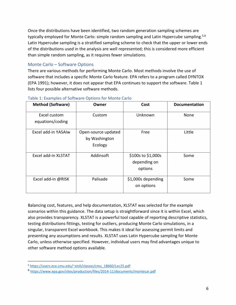
Monte Carlo – Software Options There are various methods for performing Monte Carlo. Most methods involve the use of

software that includes a specific Monte Carlo feature. EPA refers to a program called DYNTOX

(EPA 1991); however, it does not appear that EPA continues to support the software. Table 1

lists four possible alternative software methods.

Table 1: Examples of Software Options for Monte Carlo

Method (Software) Owner Cost Documentation

Excel custom

equations/coding

Custom Unknown None

Excel add-in YASAIw Open-source updated

by Washington

Ecology

Free Little

Excel add-in XLSTAT Addinsoft $100s to $1,000s

depending on

options

Some

Excel add-in @RISK Palisade $1,000s depending

on options

Some

Balancing cost, features, and help documentation, XLSTAT was selected for the example

scenarios within this guidance. The data setup is straightforward since it is within Excel, which

also provides transparency. XLSTAT is a powerful tool capable of reporting descriptive statistics,

testing distributions fittings, testing for outliers, producing Monte Carlo simulations, in a

singular, transparent Excel workbook. This makes it ideal for assessing permit limits and

presenting any assumptions and results. XLSTAT uses Latin Hypercube sampling for Monte

Carlo, unless otherwise specified. However, individual users may find advantages unique to

other software method options available.

5 https://users.ece.cmu.edu/~xinli/classes/cmu_18660/Lec25.pdf 6 https://www.epa.gov/sites/production/files/2014-11/documents/montecar.pdf

https://users.ece.cmu.edu/~xinli/classes/cmu_18660/Lec25.pdf

https://www.epa.gov/sites/production/files/2014-11/documents/montecar.pdf

7

SECTION 2: Monte Carlo - General Process Monte Carlo requires additional data and time compared to the RPA Workbook; but it also can

provide a more accurate assessment of conditions. This section describes a general process for

using Monte Carlo for RPTE and setting effluent limitations (if needed) for a parameter. To

begin, a POTW should determine and clearly state the purpose and scope of the analysis. AIC

suggests keeping the analysis as simple as possible and only adding sophistication, if required,

to avoid unnecessary variability and uncertainty.

The first step is to discuss the applicability of Monte Carlo analysis with DEQ’s IPDES Bureau.

The second step of the general process includes compiling the necessary data. There may also

be a need to review the data to remove outliers, periods of non-typical performance, and/or

other unrepresentative data. Any consideration of removing outliers or non-representative

data should be discussed with the DEQ ahead of conducting the Monte Carlo analysis. Statistics

of the data must also be calculated to summarize the data and for use in the analyses. An

analyst’s review of whether there is sufficient monitoring data available for Monte Carlo

involves an assessment of the number of samples available, coupled with the degree of

variability.7 If the analyst needs more samples, consider expanding the monitoring program to

collect additional data.

The general process described involves using the RPA Workbook and extending the analysis

with the use of Monte Carlo. Thus, the descriptions alternate between the RPA Workbook and

the additional Monte Carlo. The results of each step are important for subsequent steps.

The RPTE should be calculated using the RPA Workbook first (i.e., calculating an RPTE with a

conservative one-value mass balance). If the RPA Workbook reveals no RPTE (i.e., a WQBEL is

not needed), then the process may be stopped. If the result demonstrates that there is an RPTE

(i.e., a WQBEL is needed), the analyst should perform Monte Carlo and use the results to

evaluate the RPTE. However, there may be intermediate steps or statistical evaluations that

could be done to ascertain whether the facility’s effluent needs to be evaluated on a seasonal

basis or other statistics support the use of Monte Carlo. Jumping from the RPA workbook

evaluation directly to Monte Carlo may not be prudent.

If either or both the RPA Workbook and Monte Carlo indicate RPTE, the analyst calculates

effluent limits. Multiple Monte Carlo simulations must be performed to develop the long-term

average of the effluent parameter concentration that would meet water quality criteria (i.e.,

through an iterative process). The analyst then uses the final long-term average value to

calculate appropriate effluent limits.

7 A Statistical Power Analysis (https://www.statisticssolutions.com/statistical-power-analysis/) is one method that can be used in certain circumstances. However, this method should not be used in all cases. For additional resources, AIC suggests looking at the reports listed in the References and Resources section, and possibly obtaining additional guidance from a trained statistician.

https://www.statisticssolutions.com/statistical-power-analysis/

8

The subsections below describe the steps a general process for RPTE and effluent limits using

the RPA Workbook and Monte Carlo.

Step 1: Data Compilation Compile the necessary data for the analysis. Start with a data compilation as necessary for using

the RPA Workbook. If needed, the analyst should perform additional preparation of time series

data for Monte Carlo. Necessary time series data include the following.

• Receiving Body

o Flow

o Pollutant concentration

o Additional parameters, as needed such as hardness, pH, temperature

• Facility Effluent

o Flow

o Pollutant concentration

An analyst compiled data from a POTW to create the example shown. These data represent a

final population where the analyst has reviewed the data and determined it to be valid (i.e.,

outliers removed and data are representative), as described in Step 2. Thorough

documentation and consultation with DEQ is recommended prior to the removal of any data.

Table 2 shows the summary statistics of the time series data for the receiving body flow. Table

3 shows the flow and parameter characteristics of the time series data for the receiving body.

Table 4 shows the facility effluent characteristics. The time series and summaries shown in the

tables provide sufficient data to perform the calculations in the RPA Workbook and Monte

Carlo.

9

Table 2: Receiving Body River Flow Statistics

Statistics October – April

Count 1,061

Minimum 177

Median 282

Average 912

90th Percentile 1,810



99.70% 6,495.81

Maximum 8,540

Standard Deviation 1,861

CV 2

Table 3. Receiving Body River Characteristics

Parameter October - April

Flow 1Q10 (cfs) 60

Flow 7Q10 (cfs) 78

Flow 30Q10 (cfs) 90

Flow 30Q5 (cfs) 109

Harmonic Mean Flow (cfs) 332

Temperature, °C (95th percentile) 15.8

pH, S.U. (95th percentile) 8.81

Ammonia (ug/L) (90th percentile) 11.86

Ammonia (ug/L) (average) 7.03

Ammonia (ug/L) (standard deviation) 3.65

10

Table 4. Facility Effluent Characteristics

Parameter October - April

Flow (cfs) (average) 26.1

Flow (cfs) (standard deviation) 2.9

Ammonia (ug/L) (95th percentile) 1,132

Ammonia (ug/L) (average) 670

Ammonia (ug/L) (standard deviation) 361

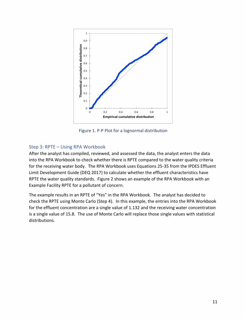
Step 2: Representative Data and Distributions The analyst should review the data for issues, such as outliers, etc. (DEQ 2017) prior to using

the RPA Workbook or performing Monte Carlo. Some additional review may be necessary for

the data time series. Excel and XLSTAT provide tools for calculating statistics on the time series.

The lognormal distribution is generally a good assumption for environmental data although the

analyst may examine alternative distributions. Considerations may include the underlying

physical processes or mechanisms determining the variable. The probability-probability (P-P)

and quantile-quantile plots may be used for comparison. These plots are found in XLSTAT

under Visualizing data -> Univariate plots -> Charts (1). For example, a test resulted in the

“best” distribution identified by XLSTAT as Weibull (2), but there is no physical mechanism to

support this and examination of the P-P plot (Figure 1) shows that the example data fits a

lognormal distribution well. The analyst should not use the goodness-of-fit test as the final

determination of distribution. The analyst should use due diligence in selecting the

distribution, even if the assessment results in the default selection of a lognormal distribution.

11

Figure 1. P-P Plot for a lognormal distribution

Step 3: RPTE – Using RPA Workbook After the analyst has compiled, reviewed, and assessed the data, the analyst enters the data

into the RPA Workbook to check whether there is RPTE compared to the water quality criteria

for the receiving water body. The RPA Workbook uses Equations 25-35 from the IPDES Effluent

Limit Development Guide (DEQ 2017) to calculate whether the effluent characteristics have

RPTE the water quality standards. Figure 2 shows an example of the RPA Workbook with an

Example Facility RPTE for a pollutant of concern.

The example results in an RPTE of “Yes” in the RPA Workbook. The analyst has decided to

check the RPTE using Monte Carlo (Step 4). In this example, the entries into the RPA Workbook

for the effluent concentration are a single value of 1.132 and the receiving water concentration

is a single value of 15.8. The use of Monte Carlo will replace those single values with statistical

distributions.

0

0.1

0.2

0.3

0.4

0.5

0.6

0.7

0.8

0.9

1

0 0.2 0.4 0.6 0.8 1

Th

eo

reti

cal cu

mu

lati

ve d

istr

ibu

tio

n

Empirical cumulative distribution

12

Figure 2. Example of RPA Workbook with an Example Facility RPTE for a Pollutant of Concern

Step 4: RPTE – Using Monte Carlo: The Mixing Equation Calculating the RPTE using Monte Carlo requires some initial steps. The analyst has compiled,

reviewed, and assessed the data (Step 1), calculated summary statistics (Step 1) and checked

the data representativeness (Step 2) and the data distributions (Step 2). The analyst has the

data prepared with the distributions for the input parameters determined and the statistical

properties of those distributions identified.

The analyst must prepare the equation for Monte Carlo. The example and description here

used XLSTAT (as described in Section 1). The simple mass balance mixing equation using the

Pollutant

of Concern

13

input distributions was set-up in the Monte Carlo format to evaluate the pollutant

concentration in the receiving water.

The mixing equation is as follows:

𝑀𝑋 =(𝑀𝑍 ∗ 𝑄𝑅 ∗ 𝐶𝑅) + (𝑄𝐸 ∗ 𝐶𝐸)

(𝑀𝑍 ∗ 𝑄𝑅) + 𝑄𝐸

MX = Result variable, final pollutant concentration

MZ = 0.25; mixing zone8

QR = Receiving water flow

CR = Receiving water pollutant concentration

QE = Facility effluent flow

CE = Facility effluent pollutant concentration

Each of the input parameters (QR, CR, QE, and CE) has a distribution. These distributions are the

variables used to define the mixing equation in XLSTAT using the average and standard

deviation. Therefore, the mixing equation for Monte Carlo is the following:

25% X QR X CR + QE X CE ___________________________________________________________ = MX

QR + QE

A single cell in XLSTAT is used to define the distribution for each input parameter. For example,

the analyst defined QR as a lognormal distribution, a mean of 2.62 and a standard deviation of

0.41 (the quantitative statistics from the log of the data). The analyst entered the data into a

distribution pop-up window as seen in Figure 3. Defining a distribution for Monte Carlo in

XLSTAT. This is found under Advanced features -> Monte Carlo Simulations -> Define a

distribution. The analyst repeated this process for each input variable.

8 The use of a 25% mixing zone is an illustrative example. DEQ is not automatically authorizing 25% mixing as EPA has done in the past. DEQ plans allocate an appropriate dilution ratio / percentage appropriate for the receiving water and discharger.

14

Figure 3. Defining a distribution for Monte Carlo in XLSTAT

Step 5: RPTE – Using Monte Carlo: The Result Variable After the analyst has defined the input variables and mixing equation (Step 4), the analyst must

define the result variable. The mixing equation is entered into the result cell, then Advanced

features -> Monte Carlo Simulations -> Define a result variable is selected, as seen in Figure 4.

The analyst provides an appropriate variable name. The corresponding function call to XLSTAT

will be inserted into the active cell.

Figure 4. Defining a result variable for Monte Carlo in XLSTAT

15

After parameters have been defined, the simulation can be run through Advanced features ->

Monte Carlo Simulations -> Run. This is when the number of simulations is defined, as seen in

Figure 5.

Figure 5. Running a Monte Carlo in XLSTAT

The Latin Hypercube method divides the distribution function of the variable into groups of

data of the same size and then generates equally sized samples within each section. This leads

to a faster convergence of the simulation. The choice of sampling method may be an option

within the software being used and may be selected based on user preference and simulation

time.

For this example, the simulation computed 26,280 results (365 days x 3 years x 24 hrs/day)

calculated from randomly selected input parameters based on the determined distributions.

Figure 6 (top half) shows a portion of the simulation results in tabular form, showing the

randomly generated input variables and the associated result variable. Note that these results

are the log of the actual predicted concentration, and this data was transformed to reflect

pollutant concentrations. Figure 6 (bottom half) shows the simulation results in graphical form

as the black line denoted at CM or mixed (receiving water and facility effluent) pollutant

concentration distribution.

16

CM

Figure 6. Monte Carlo simulation results

Step 6: RPTE – Using Monte Carlo

Monte Carlo provides a mixed (receiving water and facility effluent) pollutant concentration

distribution (CM) (Step 5). For the analyst to determine RPTE, the analyst must compare CM to

the water quality criteria for the pollutant. The critical criteria value is the lowest applicable

water quality criteria. Figure 6 (bottom half) shows three potential water quality criteria as

vertical lines (solid red, long dashed yellow, and short dashed green).

The following demonstrates how to compare the CM to the water quality criteria for

determining RPTE:

a) If the red solid line represents the critical criteria value, then much of the data

distribution is greater and the RPA Workbook result is “yes, a WQBEL is needed.”

b) If the yellow dashed line represents the critical criteria, either acute or chronic, then

95% of the data distribution is less and the RPA Workbook result is close, but “no, a

WQBEL is not needed.”

17

c) If the green dotted line represents the critical criteria, then the data distribution is less

and the RPA Workbook result demonstrates that “no, a WQBEL is not needed.”

Step 7: Effluent Limits – Using RPA Workbook If RPTE in RPA Workbook results in “Yes” (Step 3, Figure 2), then the RPA Workbook will

calculate effluent limits (Figure 7). Note the RPA Workbook calculates an average monthly limit

(AML) and a maximum daily limit (MDL). If different averaging periods are appropriate, then

the permit writer must perform additional calculations.

Figure 7. Example of RPA Workbook with an Example Facility Effluent Limits for a Pollutant of

Concern

Step 8: Effluent Limits – Using Monte Carlo Calculating effluent limits using Monte Carlo requires iterations of simulations. The analyst

creates these iterations by altering the probability distribution of the effluent concentrations.

This is done by altering the average effluent concentration used in the mixing analysis, since

this is one of the parameters that defines the probability distribution (see Step 4). The Monte

Carlo results are different mixed distributions.

The analyst uses Monte Carlo to calculate the best-fit effluent long-term average, given the

distribution that results in a mixed 95th percentile corresponding to the criteria. The analyst

finds this value by testing various effluent concentrations, simulated using the Monte Carlo

distributions, and then checking to see whether the resulting mixed 95th percentile is above or

below the water quality criteria. The analyst repeats the process until achieving the best-fit

effluent long-term average.

The analyst uses the long-term average resulting from the iterations to calculate the effluent

limits. For example, if average monthly and maximum daily effluent limits are necessary and

18

appropriate, then the permit writer uses the standard average monthly and maximum daily

equations (as shown below) with the data CV and Monte Carlo found long-term average to

calculate effluent limits. A non-toxic parameter may be more appropriately limited by using

seasonal or average monthly limits and may not include a maximum daily limit.

𝐴𝑣𝑒𝑟𝑎𝑔𝑒 𝑀𝑜𝑛𝑡ℎ𝑙𝑦 𝐿𝑖𝑚𝑖𝑡 = 𝐿𝑇𝐴 ∗ 𝑒1.645√ln(𝐶𝑉2

𝑛+1⁄ )−0.5 ln(𝐶𝑉2

𝑛+1⁄ )

𝑀𝑎𝑥𝑖𝑚𝑢𝑚 𝐷𝑎𝑖𝑙𝑦 𝐿𝑖𝑚𝑖𝑡 = 𝐿𝑇𝐴 ∗ 𝑒2.326√ln(𝐶𝑉2+1)−0.5 ln(𝐶𝑉2+1)

LTA = Long-term average

CV = coefficient of variation

Step 9: Effluent Limits – RPA Workbook versus Monte Carlo The POTW should compare the potential effluent limits based on the outcomes of the RPA

Workbook and Monte Carlo. As stated in the Introduction, Monte Carlo does not guarantee

different effluent limits, and may provide either less or more stringent treatment requirements

to meet water quality criteria within the receiving water body. If the Monte Carlo result is less

stringent effluent limits, defensible based on the data and distributions, then AIC recommends

the POTW pursue this methodology with DEQ. Note this requires the POTW understand the

data collected and perform the calculations in the steps above to understand the appropriate

strategy to pursue during the POTW permit renewal period.

19

SECTION 3: Monte Carlo – Illustrative Examples The general process for the analysis was used with data examples to demonstrate some of the

various applications of Monte Carlo. Data for the examples provided below are based upon

information shared by Idaho municipalities. Data were reviewed for outliers and non-typical

performance periods were removed. These examples are meant only for demonstrative

purposes. Anomalies could still exist in the data. The POTWs have not reviewed the compiled

data or the analysis. These data and examples have not been included in part or in whole for

any DEQ IPDES permit applications, permits, and/or other submittals.

Monte Carlo Example – Facility P

Facility P - Data Compilation

Facility P discharges to River Q. The flow for River Q based on the records from the nearest

USGS gage is shown in Table 5. Information about River Q is shown in Table 6. Information

about Facility P is shown in Table 7. Facility P Characteristics

Table 5. River Q USGS Flow Gage Statistics

Statistics Annual July - October November - June

Count 38,820 13,100 25,720

Minimum 0.2 0.2 2

Median 230 98 280

Average 269 123 343

90th Percentile 509 253 626


99th Percentile 1,160 422 1,220

99.70% 946 394 1,056

Maximum 2,850 721 2,850

Standard Deviation 226 90 237

CV 0.84 0.73 0.69

20

Table 6. River Q Characteristics

Parameter July - October November - June

Flow 1Q10 (cfs) 53 87

Flow 7Q10 (cfs) 69 109

Flow 30Q10 (cfs) 80 132

Flow 30Q5 (cfs) 95 159

Harmonic Mean Flow (cfs) 193 196

Hardness, as mg/L CaCO3 (5th

percentile)

185 185

Temperature, °C (95th percentile) 21 16

pH, S.U. (95th percentile) 7.6 7.8

Ammonia (ug/L) (90th percentile) 60 60

Ammonia (ug/L) (average) 23.6 23.6

Ammonia (ug/L) (standard deviation) 20 20

Ammonia (ug/L) (CV) 0.85 0.85

Zinc (ug/L) (90th percentile) 16.4 16.4

Zinc (ug/L) (average) 11.0 11.0

Zinc (ug/L) (standard deviation) 6.4 6.4

Zinc (ug/L) (CV) 0.58 0.58

21

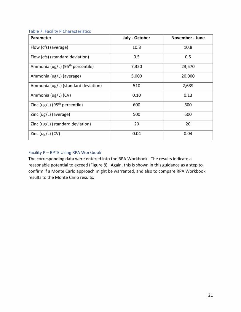
Table 7. Facility P Characteristics

Parameter July - October November - June

Flow (cfs) (average) 10.8 10.8

Flow (cfs) (standard deviation) 0.5 0.5

Ammonia (ug/L) (95th percentile) 7,320 23,570

Ammonia (ug/L) (average) 5,000 20,000

Ammonia (ug/L) (standard deviation) 510 2,639


Zinc (ug/L) (95th percentile) 600 600

Zinc (ug/L) (average) 500 500

Zinc (ug/L) (standard deviation) 20 20

Zinc (ug/L) (CV) 0.04 0.04

Facility P – RPTE Using RPA Workbook

The corresponding data were entered into the RPA Workbook. The results indicate a

reasonable potential to exceed (Figure 8). Again, this is shown in this guidance as a step to

confirm if a Monte Carlo approach might be warranted, and also to compare RPA Workbook

results to the Monte Carlo results.

22

Figure 8. Facility P RPTE Results from RPA Workbook

Facility P – RPTE Using Monte Carlo

Using the average and standard deviation values with a 25% mixing zone,9 the mixing equation

was used with Monte Carlo. The simulation computed 26,280 results. The results indicate that

there could be a reasonable potential to exceed (Table 8).

9 A 25% MZ is used here as an illustrative example. DEQ’s MZ policy is to evaluate MZ on an incremental, iterative basis; potentially starting from a 0% MZ rather than applying a default 25% MZ.

Examples show default CV

for simplicity. For actual

calculations, follow ELDG

that states for n<12 use

0.6 otherwise use

calculated value.

23

Table 8. Facility P RPTE results using Monte Carlo

Parameter Effluent Concentration (CE)

Tested in Monte Carlo (ug/L)

July - October November - June

Ammonia (ug/L) 82 No No

100 No No

300 No No

706 No No

1,000 No No

3,000 No No

5,000 Yes No

30,000 Yes Yes

Zinc (ug/L) 5 No No

35 No No

75 No No

100 No No

125 No No

250 No No

350 Yes No

500 Yes Yes

Facility P – Effluent Limits Using RPA Workbook

Given the results indicate a reasonable potential to exceed, the effluent limitations are

calculated in the RPA Workbook (Figure 9).

24

Figure 9. Facility P Effluent Limits from RPA Workbook

Facility P - Effluent Limits Using Monte Carlo

A range of effluent limitations are tested with the Monte Carlo simulations to develop a curve

and find the intersection point with the water quality criteria (Figure 10 and Figure 11). The

intersection point represents the long-term average of a distribution that meets the water

quality criteria (Step 8).



calculations, consult with

DEQ on CV selection.

25

Figure 10. Results of a Range of Effluent Concentrations from Monte Carlo, Ammonia

y = 0.605x + 264.27R² = 0.9999

0

2,000

4,000

6,000

8,000

10,000

12,000

0 5,000 10,000 15,000 20,000 25,000 30,000

Mix

ed C

on

dit

ion

(u

g/L)

Effluent (ug/L)

July - October Ammonia

Monte Carlo Result

WQ Criteria Acute

WQ Criteria Chronic

Linear (Monte Carlo Result)

y = 0.2343x + 965.14R² = 0.9998

0

2,000

4,000

6,000

8,000

10,000

12,000

0 5,000 10,000 15,000 20,000 25,000 30,000

Mix

ed C

on

dit

ion

(u

g/L)

Effluent (ug/L)

November - June Ammonia

Monte Carlo Result

WQ Criteria Acute

WQ Criteria Chronic


26

Figure 11. Results of a Range of Effluent Concentrations from Monte Carlo, Zinc

Facility P - Effluent Limits RPA Workbook versus Monte Carlo

A comparison of WQBELs using the steady state approach in the RPA Workbook and Monte

Carlo are shown in (Table 9).

y = 0.6378x + 11.513R² = 0.9983

0

20

40

60

80

100

120

140

160

180

200

0 100 200 300 400 500 600 700 800 900 1,000

Mix

ed C

on

dit

ion

(u

g/L)

Effluent (ug/L)

July - October Zinc

Monte Carlo Result

WQ Criteria Acute

WQ Criteria Chronic


y = 0.3812x + 13.048R² = 0.9972

0

20

40

60

80

100

120

140

160

180

200

0 100 200 300 400 500 600 700 800 900 1,000

Mix

ed C

on

dit

ion

(u

g/L)

Effluent (ug/L)

November - June Zinc

Monte Carlo Result

WQ Criteria Acute

WQ Criteria Chronic


27

Table 9. Comparison of Potential Effluent Limitations

Method Limit Ammonia Zinc

July -

October

November

- June

July -

October

November -

June

RPA Average Monthly Limit (AML),

mg/L

6.8 9.0 0.22 0.28

Maximum Daily Limit (MDL),

mg/L

17.8 23.6 0.37 0.48

Monte

Carlo

Average Monthly Limit (AML),

mg/L

4.6 9.8 0.53 0.88


mg/L

14.1 29.9 1.07 1.77

For Facility P, the RPTE using both the steady state RPA Workbook and Monte Carlo reveals

effluent limitations are necessary for ammonia and zinc. The Monte Carlo calculated effluent

limitations are higher for both seasons for zinc and for the November through June period for

ammonia. The differences are small and likely would not change facility planning or process

implementation, but could provide an additional margin for meeting compliance for Facility P.

28

Monte Carlo Example – Facility C

Facility C - Data Compilation

Facility C discharges to River S. The flow for River S based on the records from the nearest

USGS gage is shown in Table 10. Information about River S is shown in Table 11. Information

about Facility C is shown in Table 12.

Table 10. River S USGS Flow Gage Statistics

Statistics Annual July - September October - June

Count 38,491 9,660 28,831

Minimum 67 64 4,750

Median 3,100 1,160 24,041

Average 6,251 1,397 24,004

90th Percentile 17,200 2,280 39,437

95th Percentile 21,100 3,200 41,339

99th Percentile 29,500 6,962 42,860

99.70% 27,112 5,480 57,379

Maximum 49,800 17,900 43,241

Standard Deviation 6,954 1,361 11,125

CV 1.11 0.97 0.46

29

Table 11. River S Characteristics

Parameter July - September October - June

Flow 1Q10 (cfs) 248 890

Flow 7Q10 (cfs) 292 1,030

Flow 30Q10 (cfs) 363 1,270

Hardness, as mg/L CaCO3 (5th

percentile)

19.2 19.2

Temperature, °C (95th percentile) 25 18.4

pH, S.U. (95th percentile) 6.6 6.6

Ammonia (ug/L) (90th percentile) 250 250

Ammonia (ug/L) (average) 100 100






Zinc (ug/L) (CV) 1 1

30

Table 12. Facility C Characteristics

Parameter July - September October - June





Ammonia (ug/L) (standard deviation) 2,968 6,514





Zinc (ug/L) (CV) 0.75 0.75

Facility C – RPTE Using RPA Workbook

The corresponding data were entered into the RPA Workbook. The results indicate a reasonable

potential to exceed (Figure 12).

31

Figure 12. Facility C RPTE Results from RPA Workbook





0.6 otherwise use

calculated value.

32

Facility C - RPTE Using Monte Carlo

Using the average and standard deviation values with a 25% mixing zone, the mixing equation

was used in Monte Carlo. The simulation computed 26,280 results. The results indicate that


Table 13. Facility C RPTE results using Monte Carlo


Tested in Monte Carlo

(ug/L)

July - September October - June

Ammonia (ug/L) 3,000 No No

7,500 No No

10,000 No No

17,441 No No

30,000 No No

50,000 Yes No

100,000 Yes No

500,000 Yes Yes

Zinc (ug/L) 5 No No

10 No No

75 Yes No

201 Yes No

500 Yes No

1,000 Yes No

2,500 Yes Yes

5,000 Yes Yes

33

Facility C - Effluent Limits Using RPA Workbook



Figure 13. Facility C Effluent Limits from RPA Workbook

Facility C - Effluent Limits Using Monte Carlo









34


y = 0.0839x + 120.13R² = 0.9999

0

5,000

10,000

15,000

20,000

25,000

30,000

35,000

0 500,000 1,000,000 1,500,000 2,000,000 2,500,000

Mix

ed C

on

dit

ion

(u

g/L)

Effluent (ug/L)

July - September Ammonia

Monte Carlo Result

WQ Criteria Acute

WQ Criteria Chronic


y = 0.015x + 64.8R² = 1

0

5,000

10,000

15,000

20,000

25,000

30,000

35,000

0 500,000 1,000,000 1,500,000 2,000,000 2,500,000

Mix

ed C

on

dit

ion

(u

g/L)

Effluent (ug/L)

October - June Ammonia

Monte Carlo Result

WQ Criteria Acute

WQ Criteria Chronic


35


Facility C - Effluent Limits RPA Workbook versus Monte Carlo

A comparison of long-term average (LTA) effluent limitations from the RPA Workbook and

Monte Carlo are shown in (Table 14). The long-term average (LTA) is used to calculate the

limits.

y = 0.1747x + 12.285R² = 0.9993

0

5

10

15

20

25

30

0 500 1,000 1,500 2,000 2,500

Mix

ed C

on

dit

ion

(u

g/L)

Effluent (ug/L)

July - September Zinc

Monte Carlo Result

WQ Criteria Acute

WQ Criteria Chronic


y = 0.0155x + 2.6792R² = 0.999

0

5

10

15

20

25

30

0 500 1,000 1,500 2,000 2,500

Mix

ed C

on

dit

ion

(u

g/L)

Effluent (ug/L)

October - June Zinc

Monte Carlo Result

WQ Criteria Acute

WQ Criteria Chronic


36



July -

September

October -

June

July -

September

October -

June


mg/L

13.0 13.0 0.07 0.22


mg/L

34.0 34.0 0.18 0.57

Monte

Carlo


mg/L

46 n/a 0.17 3.05


mg/L

139 n/a 0.35 6.16

For Facility C, the RPTE using both the RPA Workbook and Monte Carlo reveals effluent

limitations are necessary for zinc, but may only be necessary for July through September for

ammonia given current treatment levels. The Monte Carlo calculated effluent limitations are

higher for ammonia and zinc. Facility C is exceeding the necessary treatment levels with the

current effluent limitations so no tightening of limits is needed.

37

Monte Carlo Example – Facility M

Facility M - Data Compilation

Facility M discharges to River F. The flow for River F based on the records from the nearest

USGS gage is shown in Table 15. Information about River F is shown in Table 16. Information

about Facility M is shown in Table 17.

Table 15. River F USGS Flow Gage Statistics

Statistics Annual October - April May - September

Count 539 364 175

Minimum 15.7 15.7 85.9

Median 42 31 144

Average 85 54 149




99.70% 277 207 252

Maximum 279 223 279

Standard Deviation 64 51 35

CV 0.76 0.94 0.23

38

Table 16. River F Characteristics

Parameter October - April May - September

Flow 1Q10 (cfs) 1.4 28

Flow 7Q10 (cfs) 1.8 36.5

Flow 30Q10 (cfs) 2.0 40.1

Hardness, as mg/L CaCO3 10 10

Temperature, °C 16.1 22

pH, S.U. 8.8 8.8

Ammonia (ug/L) (90th percentile) 1.2 1.2



Ammonia (ug/L) (CV) n/a n/a




Zinc (ug/L) (CV) n/a n/a

39

Table 17. Facility M Characteristics

Parameter October - April May - September





Ammonia (ug/L) (standard deviation) 10,401 15,007





Zinc (ug/L) (CV) 0.17 0.17

Facility M – RPTE Using RPA Workbook

The corresponding data were entered into the RPA Workbook. The results indicate a reasonable

potential to exceed (Figure 16).

40

Figure 16. Facility M RPTE Results from RPA Workbook





0.6 otherwise use

calculated value.

41

Facility M - RPTE Using Monte Carlo




Table 18. Facility M RPTE results using Monte Carlo



October - April May - September

Ammonia (ug/L) 0.01 No No

0.1 No No

1.0 No No

10 No No

100 No No

1,000 Yes Yes

7,825 Yes Yes

10,000 Yes Yes

Zinc (ug/L) 0.0001 No No

0.001 No No

0.01 No No

0.1 No Yes

1 No Yes

10 Yes Yes

150 Yes Yes

1,000 Yes Yes

42

Facility M - Effluent Limits Using RPA Workbook



Figure 17. Facility M Effluent Limits from RPA Workbook





43

Facility M - Effluent Limits Using Monte Carlo






y = 2.1226x + 0.9089R² = 1

0

200

400

600

800

1,000

1,200

1,400

1,600

1,800

2,000

0 200 400 600 800 1,000 1,200 1,400

Mix

ed C

on

dit

ion

(u

g/L)

Effluent (ug/L)

May - September Ammonia

Monte Carlo Result

WQ Criteria Acute

WQ Criteria Chronic


y = 0.9396x + 3.0351R² = 1

0

200

400

600

800

1,000

1,200

1,400

1,600

1,800

2,000

0 200 400 600 800 1,000 1,200 1,400

Mix

ed C

on

dit

ion

(u

g/L)

Effluent (ug/L)

October - April Ammonia

Monte Carlo Result

WQ Criteria Acute

WQ Criteria Chronic


44


Facility M - Effluent Limits RPA Workbook versus Monte Carlo


Monte Carlo are shown in (Table 19). The long-term average (LTA) is used to calculate the

limits.

0

2

4

6

8

10

12

14

16

18

20

0.0 0.5 1.0 1.5 2.0 2.5 3.0 3.5 4.0 4.5 5.0

Mix

ed C

on

dit

ion

(u

g/L)

Effluent (ug/L)

May - September Zinc

Monte Carlo Result

WQ Criteria Acute

WQ Criteria Chronic

0

2

4

6

8

10

12

14

16

18

20

0.0 0.5 1.0 1.5 2.0 2.5 3.0 3.5 4.0 4.5 5.0

Mix

ed C

on

dit

ion

(u

g/L)

Effluent (ug/L)

October - April Zinc

Monte Carlo Result

WQ Criteria Acute

WQ Criteria Chronic

45



October -

April

May -

September

October

- April

May -

September


mg/L

0.5 0.7 0.019 0.019


mg/L

1.3 1.9 0.049 0.049

Monte

Carlo


mg/L

n/a 0.5 0.002 0.004


mg/L

n/a 1.6 0.004 0.007

For Facility M, the RPTE using both the RPA Workbook and Monte Carlo reveals effluent

limitations are necessary for zinc, but may only be necessary for May through September for

ammonia given current treatment levels. The Monte Carlo calculated effluent limitations are

lower than the RPA Workbook limits. Facility M has some high variability in these effluent

parameters leading to the lower Monte Carlo results. The compiled data for Facility M may

need to be further screened to examine if less variability can be achieved long-term.

46

Monte Carlo Example – Facility B

Facility B - Data Compilation

Facility B discharges to River B. The flow for River B based on the records from the nearest

USGS gage is shown in Table 20. Information about River B is shown in Table 21. Information

about Facility B is shown in Table 22.

Table 20. River B USGS Flow Gage Statistics

Statistics Annual May - September October - April

Count 28,303 12,254 16,049

Minimum 2 50 2

Median 2,360 4,170 774

Average 2,865 4,461 1,647

90th Percentile 6,650 8,100 5,170

95th Percentile 8,440 9,734 7,090

99th Percentile 11,200 12,300 9,300

99.70% 11,062 11,776 8,486

Maximum 19,700 18,700 19,700

Standard Deviation 2,732 2,438 2,280

CV 0.95 0.55 1.38

47

Table 21. River B Characteristics

Parameter May - September October - April

Flow 1Q10 (cfs) 265 111

Flow 7Q10 (cfs) 285 127

Flow 30Q10 (cfs) 384 140

Flow 30Q5 (cfs) 457 163

Harmonic Mean Flow (cfs) 398 391

Hardness, as mg/L CaCO3 36 40

Temperature, °C 18.7 14.1

pH, S.U. 8.9 8.6








Zinc (ug/L) (CV) 0.33 0.33

48

Table 22. Facility B Characteristics

Parameter May - September October - April

Flow (cfs) (average) 31 31

Flow (cfs) (standard deviation) 2 2








Zinc (ug/L) (CV) 0.33 0.33

Facility B – RPTE Using RPA Workbook

The corresponding data were entered into the RPA Workbook. The results indicate a

reasonable potential to exceed (Figure 20).

49

Figure 20. Facility B RPTE Results from RPA Workbook

Facility B - RPTE Using Monte Carlo








0.6 otherwise use

calculated value.

50

Table 23. Facility B RPTE results using Monte Carlo



May - September October - April

Ammonia (ug/L) 0.1 No No

1 No No

5 No No

10 No No

100 No No

670 No No

1,000 No No

10,000 Yes Yes

Zinc (ug/L) 0.01 No No

0.1 No No

1 No No

10 No No

25 No No

75 No No

100 Yes No

2,000 Yes Yes

51

Facility B - Effluent Limits Using RPA Workbook


calculated in the RPA worksheet (Figure 21).

Figure 21. Facility B Effluent Limits from RPA Workbook





52

Facility B - Effluent Limits Using Monte Carlo






y = 0.1012x + 28.011R² = 0.9989

0

200

400

600

800

1,000

1,200

1,400

1,600

1,800

2,000

0 1,000 2,000 3,000 4,000 5,000 6,000 7,000 8,000 9,000 10,000

Mix

ed C

on

dit

ion

(u

g/L)

Effluent (ug/L)

May - September Ammonia

Monte Carlo Result

WQ Criteria Acute

WQ Criteria Chronic


y = 0.2799x + 86.103R² = 0.9983

0

200

400

600

800

1,000

1,200

1,400

1,600

1,800

2,000

0 1,000 2,000 3,000 4,000 5,000 6,000 7,000 8,000 9,000 10,000

Mix

ed C

on

dit

ion

(u

g/L)

Effluent (ug/L)

October - April Ammonia

Monte Carlo Result

WQ Criteria Acute

WQ Criteria Chronic


53


Facility B - Effluent Limits RPA Workbook versus Monte Carlo


Monte Carlo are shown in (Table 24Error! Reference source not found.). The long-term

average (LTA) is used to calculate the limits.

0

5

10

15

20

25

30

35

40

45

50

0 20 40 60 80 100 120 140 160 180 200

Mix

ed C

on

dit

ion

(u

g/L)

Effluent (ug/L)

May - September Zinc

Monte Carlo Result

WQ Criteria Acute

WQ Criteria Chronic

0

5

10

15

20

25

30

35

40

45

50

0 20 40 60 80 100 120 140 160 180 200

Mix

ed C

on

dit

ion

(u

g/L)

Effluent (ug/L)

October - April Zinc

Monte Carlo Result

WQ Criteria Acute

WQ Criteria Chronic

54



May -

September

October -

April

May -

September

October -

April


mg/L

1.1 1.1 0.05 0.03


mg/L

2.8 2.8 0.14 0.09

Monte

Carlo


mg/L

4.7 3.5 0.17 0.28


mg/L

14.5 10.8 0.34 0.56

For Facility B, the RPTE using both the RPA Workbook and Monte Carlo reveals effluent

limitations are necessary for ammonia and zinc. The Monte Carlo calculated effluent limitations

are higher than the RPA Workbook limits. The differences are significant enough to potentially

even reconsider facility planning or process implementation. These higher limits should be

requested in the permit to provide an additional margin for meeting compliance for Facility B.

55

References and Resources 33 U.S.C. 1251. Federal Water Pollution Control Act [As Amended Through P.L. 107–303,

November 27, 2002]

Brouwer and DeBlois 2008. Integrated modelling of risk and uncertainty underlying the cost and effectiveness of water quality measures. Environmental Modelling & Software. Volume 23, Issues 7, July 2008, Pages 922-937.

DEQ 2002. Decision Analysis Report 2. National Pollutant Discharge Elimination System Program Review. Department of Environmental Quality November 19, 2002. Boise, ID.

DEQ 2017. Idaho Pollutant Discharge Elimination System, User’s Guide to Permitting and Compliance, Volume 1—General Information. Boise, ID.

EPA 1991. Technical Support Document for Water Quality-based Toxics Control. EPA/505/2-90-001.

EPA 1997. Guiding Principles for Monte Carlo Analysis. EPA/630/R-97/001.

EPA 2003. Elements of a State Water Monitoring and Assessment Program. EPA/841-B-03-003.

EPA 2010. U.S. EPA (2010b) NPDES Permit Writers’ Manual. U.S. Environmental Protection Agency, Office of Wastewater Management, Water Permits Division, State and Regional Branch, EPA-833-K-10-001.

King, K.W. and R.D. Harmel 2003. Considerations in Selecting a Water Quality Sampling Strategy. Vol. 46(1): 63–73 2003 American Society of Agricultural Engineers ISSN 0001–2351.

LII 2018. Cornell Law School. Legal Information Institute (LII). CFR › Title 40 › Chapter I › Subchapter H › Part 230 › Subpart A › Section 230.3. https://www.law.cornell.edu/cfr/text/40/230.3

McLaughlin, DB and CA Flinders 2016. Quantifying Variability in Four US Streams Using a Long-Term Data Set: Patterns in Water Quality Endpoints. Environ Manage.2016 Feb;57(2):368-88. doi: 10.1007/s00267-015-0609-7. Epub 2015 Sep 24.

RPT 2011. Evaluating the Water Quality Dataset. The Sustainable Future Institute, as part of Project 2058. Report 10: The State of New Zealand’s Resources.

WERF 2016. Nutrient Management Volume III: Development of Nutrient Permitting Frameworks. By David L. Clark, Tom Dupuis, Haley Falconer, Lorin Hatch, Michael S. Kasch, Paula J. Lemonds, and JB Neethling.

https://www.law.cornell.edu/cfr/text

https://www.law.cornell.edu/cfr/text/

https://www.law.cornell.edu/cfr/text/40/chapter-I

https://www.law.cornell.edu/cfr/text/40/chapter-I

https://www.law.cornell.edu/cfr/text/40/chapter-I/subchapter-H

https://www.law.cornell.edu/cfr/text/40/part-230

https://www.law.cornell.edu/cfr/text/40/part-230/subpart-A

https://www.law.cornell.edu/cfr/text/40/230.3

https://www.ncbi.nlm.nih.gov/pubmed/26404431

Documents

Data Analysis for Effluent Limitations using Monte Carlo · use of the Monte Carlo method must be justified through prior assessment of limit requirements using simpler methods. Implementing