Data Analysis Guide - TATAA Biocenter · This data analysis guide will provide an instruction on how to export data from the most common ... For ABI Viia 7, 7900, ... PCR Instruction

Data Analysis Guide

For the miRCURY LNA™ Universal RT

microRNA Ready-to-Use PCR panels

using Exiqon GenEx software Version 2.5 (January 2013)

Contents

Considerations on Normalization ................................................................................................... 4

Why normalize? ................................................................................................................................ 4

Controls and normalization assays................................................................................................ 4

Introduction to GenEx ...................................................................................................................... 6

Flow of data analysis ....................................................................................................................... 8

Export the run data from your cycler ............................................................................................. 9

Importing and merging your instrument export files using the Exiqon import wizard .............. 14

Inter-plate calibration ..................................................................................................................... 23

Quality control ................................................................................................................................. 24

Cut off ............................................................................................................................................... 28

Frequency of missing data ............................................................................................................ 29

Call rate plot .................................................................................................................................... 29

Missing data .................................................................................................................................... 30

microRNAs detected only in a subset of samples ..................................................................... 32

Normalization to global mean ....................................................................................................... 32

Normalization to reference gene(s) ............................................................................................. 33

Average RT replicates ................................................................................................................... 37

Converting to relative quantities ................................................................................................... 38

Further data analysis using GenEx ................................................................................................. 40

Using the Data manager ............................................................................................................... 41

Statistical analysis in GenEx ........................................................................................................ 42

Creating a subset of regulated assays........................................................................................ 44

Gene info ......................................................................................................................................... 51

Data analysis guide version 2.4

3

Quick steps for experienced users .................................................................................................. 52

Online help .......................................................................................................................................... 53

References .......................................................................................................................................... 53


4

The data analysis guide version 2 This data analysis guide will provide an instruction on how to export data from the most common

real-time PCR cyclers, import and annotation of data in GenEx using the Exiqon data import wizard,

and how to perform the data pre-processing. The data pre-processing described here involves steps

such as interplate calibration, setting cut-off, handling missing data points, removing outliers,

checking for sample and assay quality, averaging technical replica, normalizing to global mean or

stable reference genes (including selection), scaling and log transforming the data. The guide will

also provide a brief introduction to basic statistical analysis using either T-test or ANOVA to show

whether any of the samples are significantly different from one another, including a list of the most

regulated microRNAs across the samples. Finally, it will be mentioned how to easily create advanced

publication-ready figures such as heatmap and principal component analysis, and retrieve further

information on analyzed microRNAs from online databases.

The Exiqon data import wizard applies to data generated on miRCURY LNA™ Universal RT microRNA

Ready-to-Use PCR panels whereas GenEx data analysis module can be used for data generated on

both Ready-to-Use PCR panels as well as miRCURY LNA™ Universal RT microRNA individual assays.

Considerations on Normalization

Why normalize? The purpose of a qPCR experiment is usually the detection or verification of differential, biologically

relevant expression levels in a set of samples.

In setting up an experiment, small differences in replicate performance cannot be avoided, even

when protocols are standardized: sampling may not be identical, storage may have different effects

on each sample, RNA extraction may not be 100% reproducible, PCR inhibitors may be present in

some but not all samples, pipetting may not be accurate, and real-time cyclers may show run-to-run

variation. In order to get biologically relevant data, it is important to filter out technical variation. For

this purpose, different approaches to normalization may be employed.

Controls and normalization assays In the design of the plate-layout for the miRCURY LNA™ Universal RT microRNA PCR, Ready-to-Use

PCR panels, we have incorporated several options for data normalization.

Inter-plate calibrator

Since each assay is present only once on each plate, replicates must be performed using separate

plates. This raises the issue of run-to-run differences. To allow for simple inter-plate calibration, we

have designed a calibration assay with a companion template (annotated as UniSp3 IPC in the plate

layout files).

Three wells have been assigned for inter-plate calibration to provide triplicate values with the

possibility for outlier removal. In each of these wells, both the primers and the DNA template are


5

present, giving high reproducibility. The inter-plate calibrator is independent of cDNA quality in

order to give a signal (but may be affected by PCR inhibitors in the sample) and can therefore be

used to quality control each plate run.

Sample spike-in

Some sample types may contain PCR inhibitors, which sometimes survive RNA purification. This may

result in different reverse transcription or PCR efficiencies between compared samples. One way to

control for differences in efficiencies is by adding a known RNA spike-in to the sample during cDNA

synthesis. We have designed an RNA spike-in, UniSp6, for this purpose. The UniSp6 RNA template is

provided with the cDNA synthesis kit. One well in the Ready-to-Use PCR plates contains the

matching primer set. A UniSp6 PCR primer set is also provided with the SYBR® green master mix kit,

which is to be used with our non-plate based PCR primer set products. We do not recommend

normalizing to the synthetic spike-in – it should be used for sample quality control.

Global Mean Normalization

Variation due to sample differences and handling prior to cDNA synthesis can be normalized using

endogenously expressed miRs. In large screening studies, it is often recommendable to normalize

data against the global mean; i.e., the average of all microRNAs expressed in all samples [1]. This can

be the best option when screening samples with a high call-rate (number of expressed microRNAs)

and a high proportion of essentially unregulated microRNAs, but should be used with caution in

validation studies where most of the genes are chosen precisely for being differentially expressed.

Global normalization is also not a good option between samples in which the overall microRNA

expression level is changed.

Reference gene Normalization

The use of endogenous reference genes can be another approach to normalize against variation due

to sample differences and handling prior to cDNA synthesis. Though this is a good and

recommended approach, great caution should be taken in the selection of reference genes. The

danger of using endogenous reference genes lies in the assumption that a specific gene is expressed

at the exact same level in all sample types. This is rarely true. The selection of reference genes

should therefore be made with care, and should be specific to the sample set you are working with.

This selection can be performed using NormFinder and/or geNorm, both incorporated into GenEx.

For validation studies based on panel screening, the reference genes may be selected during the

screening process, based on expression behavior most resembling the global mean.

In our panels, we have pre-assigned 6 wells for 6 different genes which have stable expression levels

over a wide range of sample types. Three of these are microRNAs which are often stably expressed,

and the other three are small RNA reference genes. Once qPCR data has been obtained, the

appropriateness of these references can be analyzed for your specific samples and the optimal

number of references can be selected. When applicable, we recommend choosing stably expressed

microRNAs over other small RNA reference genes, since microRNA best resemble the behavior of

microRNA both biologically and during experimental handling (extraction, RT etc.)


6

How to get started with GenEx

Introduction to GenEx Exiqon has partnered with MultiD to provide a software for qPCR data analysis specifically adapted

to our miRCURY LNA™ Universal RT microRNA PCR products. GenEx offers advanced methods to

analyze real-time qPCR data with simple clicks of the mouse. The methods are suitable to select and

validate reference genes, classify samples, group genes, monitor time dependent processes and

much more.

Possibly the most important part of qPCR experiments is the pre-processing of raw data for

subsequent statistical analysis. Pre-processing steps need to be performed with consistence, in the

correct order and with confidence. GenEx has a streamlined and user-friendly interface which aids

data handling. Powerful presentation tools present professional illustrations of even the most

complex experimental designs.

GenEx is intuitive and easy to use, and with the Exiqon qPCR plate import wizard, data import and

merge becomes simple. Furthermore, GenEx has the advantage of incorporating both NormFinder

and geNorm in the software. Thus, you get both of these algorithms on which to base your choice of

reference genes in one software installation. GenEx also offers advanced statistical solutions for

post-normalization data analysis. Current features include parametric and non-parametric statistical

tests, clustering methods, principal component analysis, artificial neural networks, and much more.

Download and install GenEx

To install the Exiqon version of GenEx, go to http://www.exiqon.com/qpcr-software and the

“software download” tab.

In the dialogue box choose run, and follow the installation guide. If you have purchased a GenEx

license, use the license key provided by email. Otherwise you may use a free demo license for 30

days.

Once installed, remember to check for updates. MultiD continuously works to improve the software,

and updates are periodically released, so check for updates routinely.

The GenEx manual is available within the software under the Help menu.

http://www.exiqon.com/qpcr-software


7

Practice data set

Data for testing the Exiqon import wizard and data analysis flow can be found here: c:\program

files\Multid\Genex5\Exiqon\Examples

The folder contains a full data set of .txt files exported from panel I and II, analyzed on an LC480,

along with matching layout files. You will also find an excel file with examples of serum/plasma

values for hemolysis testing.


8

Flow of data analysis Before you get started with setting up your experiments, it may be useful to consider the shown

data analysis flow:


9

How to get the raw data from your cycler into

GenEx

Export the run data from your cycler Run your experiment according to the protocol.

Important: For ABI Viia 7, 7900, 7500, 7500 FAST and StepOnePlus users. Prior to performing the

experiment, it is possible to download run template files (.sdt files) from the Exiqon website

(http://www.exiqon.com/sds). These files specify proper cycling and critical analysis settings, and

can be used when setting up the experiment. In the SDS software, simply open the appropriate

template file and start the run.

For your own convenience, it may be useful to annotate the run with assay and sample names – but

this is not necessary for data analysis when using Exiqon Ready-to-use plates. Annotation will take

place during the data import using the wizard.

Below, we have given examples of how to export your data from some of the major cycler types.

ABI Viia 7

If you have used an ABI Viia 7 cycler for you experiment, please note that it is necessary to verify

that the data analysis settings have been correct.

First, it is important that the experiment has been run as Type: Standard Curve.

Second, it is important that you have indicated whether or not you have used ROX passive reference

dye in the experiment, and that baseline and threshold settings are set manually and correctly. For

directions on how to analyze the data, please refer to our miRCURY LNA™ Universal RT microRNA

PCR Instruction manual, tip 10. If you have used one of our run templates, the settings should be

correct – but it is always a good idea to verify that the threshold is adequately set.

Once all settings are correct and the experiment analyzed, you are ready to export the data. In the

left-hand pane (Experiment Menu), click . In the window now appearing,

choose and

. to the location you wish to export the file

to, and assign an Export File Name (if different from the automatically assigned name). Choose

. In the various tabs, make sure that only Results is selected, and that


10

empty and omitted wells are not skipped

Select All Fiels in Content . Click either at the bottom of the

window, or in the top right-hand corner of the window.

ABI 7900

If you have used an ABI 7900 cycler for you experiment, please note that it is necessary to verify that

the data analysis settings have been correct.

First, it is important that the experiment has been run as an AQ experiment, not RQ (the SDS 2.4

version of the software allows you to convert between the two formats post-run).



directions on how to analyze the data, please refer to our miRCURY LNA™ Universal RT microRNA

PCR Instruction manual, tip 10. If you have used one of our run templates, the settings should be

correct – but it is always a good idea to verify that the threshold is adequately set.

Once all settings are correct, you are ready to export the data. In the menu, choose . In

the dialog box, choose , and

. Then to the folder of your choice.

Tip: with SDS 2.4 it is possible to perform batch export without opening the files to export. In the

menu, choose . In the dialog box, choose and

the files you wish to export. Select the destination folder with , then

. Please note that this method is only valid if you are sure that all the files have been

analyzed correctly first.

ABI 7500 and StepOnePlus

If you have used an ABI 7500, 7500 FAST or StepOne cycler for you experiment, please note that it is

necessary to verify that the data analysis settings have been correct.

First, the experiment must have been run as Type: Quantitation – Standard Curve experiment. It is

possible to change the experiment type after the run.


11



directions on how to analyze the data, please refer to the miRCURY LNA™ Universal RT microRNA PCR

Instruction manual, tip 10.

Once all settings are correct, you are ready to export the data. In the menu, choose .

In the dialog box, tick only , and select

. Assign file name and location, and select

. Then .

Roche LC480

If you have used a Roche LC480 for your experiment, go to , choose the 2nd derivative

analysis method, and make sure that the Cq values have been calculated (if this has not been done

yet, press ). To export the data, right-click on the data table and choose Export table,

browse to the location where you wish the file, and save.

Tip: For high throughput, it may be worthwhile to create a macro for running the experiment and

automatically export the data at the end of the run. How to program such a macro goes beyond the

scope of this guide, and should be learned from the LC480 manual.


12

Roche LC96

If you have used a Roche LC96 for your experiment, when you add analysis choose

.

To export one file at a time, in the tab, sub tab , one of the 4 data windows

should show with the tab active. Export by right-clicking

anywhere in the table, and choose .

Alternatively, in the menu choose . Tick

and click . Select the run files for which to export data, then click and

export the data to the location of choice.

BioRad CFX

If you have a BioRad CFX cycler, you can choose to analyse either as regression or single threshold.

Once the Cq calculations have been performed, data can be exported either from the Quantification

or Quantification Data window . Simply place the cursor over

the data table in the window, right-click and in the menu popping up choose .

Browse to the folder of choice, name the file and .

BioRad iQ5

If you have used a BioRad iQ5 cycler for your experiment, we recommend verifying that the data

analysis settings (baseline and threshold) have been correct. For directions on how to analyze the

data, please refer to our miRCURY LNA™ Universal RT microRNA PCR Instruction manual, tip 10.

Once all settings are correct, you are ready to export the data. In the tab,

click . Right-click anywhere in the Results table, and choose . Browse

to your folder of choice, name the file and .


13

Stratagene Mx3000P/3005P

If you have used a Stratagene cycler for your experiment, we recommend verifying that the data

analysis settings (baseline and threshold) have been correct. For directions on how to analyze the

data, please refer to our miRCURY LNA™ Universal RT microRNA PCR Instruction manual, tip 10.

Once all settings are correct, you are ready to export the data. In the menu choose

then . Browse to your

folder of choice, name the file and .


14

Importing and merging your instrument

export files using the Exiqon import wizard

Starting the wizard:

Open GenEx.

If you have the start-up window active, close this.

Click the Exiqon qPCR plate import wizard button .

In the pop-up window, click start.


15

Step 1: Select panel type, format and instrument

The first choice to make is whether you have been running panels in 96- or 384-well format, which

cycler you have been using, and whether your panel set contains just one plate layout (Panel I), or

two plates with different layouts (Panel I and II).

You now need to import the layout file(s). This is the Excel file(s) specifying the position (well) and

type (gene of interest, reference gene etc) of assays in the plate(s). For all standard plate formats,

these Excel files can be downloaded from Exiqon’s homepage. For Pick&Mix custom panels, the

layout files are created during the plate configuration process on Exiqon’s homepage.

If you have ticked Panel I (your panel set contains only one plate layout), then only one import

window will be available. If you have ticked Panel I and II (a plateset with two different layouts), then

two import windows will be available, one for each layout.

For each layout, browse to the location of your plate layout file, and open the file.

Click

Step 2: Select instrument export files

You now need to select your instrument export files (.txt or .xml, depending on cycler type).

If you have run only one plate type (e.g.only Serum/plasma panel in 384-well layout), then a single

panel will appear for file selection.


16

Click and browse to the location where you have your files. While using

shift or ctrl for multiple file selection, select and open your files. If the file naming has not

automatically resulted in the desired file order, you can move a file up or down in the list using the

arrow buttons .

If you have run a set of plates (e.g. Human Panel I and II V2) two panes will open.

Each pane has a button. In the left pane open the files for panel I and in

the right pane open the files of panel II.


17

Important: The files for panel I and II must have the same sample order, so that the two files for the

same sample are aligned. If the file naming has not automatically resulted in the correct order, you

can move a file up or down in the list using the arrow buttons .

Click

Please note that once you click next at this step a table is created based on the imported files. It is

not possible to go back without re-starting the wizard.

Step 3: Edit sample names and add classification columns

The table generated after file import contains 4 predefined, automatically generated columns called

classification columns.

Classifier is a term used in GenEx to group samples that belong to the same category (i.e. on same

PCR plate, technical replicates, biological groups or negative controls). Sample classifiers are found in

classification columns. Classifiers are also used to identify assays used for specific purposes (i.e

reference genes and spike-in controls). In that case, the classifiers are found in classification rows,

but that function is not relevant until step 4 – step 3 deals only with sample annotation which is done

in columns.

The way a sample classifier works, is that samples belonging to the same category or group get the

same number in the classification column. For example, negative control samples should be assigned

1 in a negative control classifier, treated samples could be assigned 1 and non-treated 2 in a

treatment classifier, and RT replicates of the same RNA sample should be assigned the same number

in an RT classifier. A classification column is recognized as having a # as the first symbol in the header


18

name. If you want GenEx to consider groups in the further data analysis you need to let GenEx know

which ones these are by adding a column for each classifier.

As mentioned above, Step 3 automatically adds 4 pre-defined classification columns. The first three

automatically assigned columns should not be edited:

#FileName serves to help identify which plates/samples came from which instrument export file,

making it easier to assign correct sample names.

#Plate is a classifier identifying which samples were run on the same plate.

SampleID identifies a sample according to its position in the Exiqon plate layout file. Again, this

should make it easier to assign proper sample names.

The only pre-defined column to edit is the #SampleName. If correct sample names have not been

assigned already in the cycler, the sample name assigned by your cycler will appear (this may vary

between cycler types). Using the file name and sample ID to identify each sample, assign each

sample name to be used during further downstream analysis. This can be done by selecting and

filling each cell individually or by copy-paste from an Excel spread-sheet containing a sample

overview. The latter method requires that the plates/samples appear in the same order in the

spread-sheet as in the wizard.

It is now possible to add additional classification columns. To the extent it is relevant in your

experiment, we recommend adding classifiers to identify at least technical replicates and biological

groups. You may also choose to identify negative control samples at this point, although these may

easily be classified during the subsequent pre-processing (explained in a later section). Additional

classifications may in some cases be relevant, i.e. to identify sub-groups.

For each classifier you wish to add, just click , name the new column (starting with

#), and assign the classifications starting from 1 and onwards for each group or category. Multiple

cells can be selected using shift or ctrl, and assigned the same classifier by right-clicking and select

insert value (this function does not work for #SampleName). If you define negative control samples

at this time, they should be given the classification value 1 while unknowns are left empty or

assigned 0 in the negative control classifier. Again, copy-paste can be used if a spread-sheet has

been created with sample overview.

For the sake of keeping the overview, it is now possible to re-size the wizard window.


19

If you accidentally added too many classification columns, they can easily be removed again. Simply

select the column you wish to delete, and click . Note that the original 4 columns

are necessary, and cannot be deleted.

Once all sample names and classifiers have been assigned, click .

Step 4: Save data or Load to data editor

You are now ready to load your data into GenEx and initiate pre-processing or alternatively save the

data for later loading. During pre-processing, GenEx will need classification columns for some of the

steps. In step 4, you get a chance to verify that all sample names and necessary classification

columns have been assigned correctly before loading to GenEx and commencing the pre-processing.


20

If you scroll all the way to the right, you will see the classification columns.


21

Note that the #FileName and SampleID columns have disappeared since they have served their

purpose. Instead, two new columns have appeared automatically: #IPC and #IPC-PlateID .These are

needed for later use in interplate calibration, and since the wizard knows the position of the

interplate calibrators from the plate layout they were automatically assigned. The difference

between #Plate and #IPC-PlateID is mainly found in experiments where two plates make a pair (as in

human panel I+II). In this case #Plate identifies the plate pair after merge. #IPC-PlateID instead

identifies the individual plates, to allow for correct interplate calibration of each individual plate.

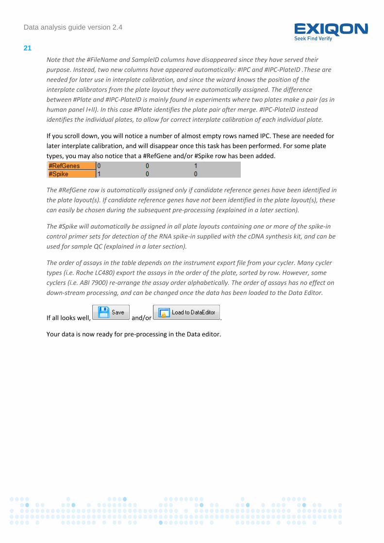
If you scroll down, you will notice a number of almost empty rows named IPC. These are needed for

later interplate calibration, and will disappear once this task has been performed. For some plate

types, you may also notice that a #RefGene and/or #Spike row has been added.

The #RefGene row is automatically assigned only if candidate reference genes have been identified in

the plate layout(s). If candidate reference genes have not been identified in the plate layout(s), these

can easily be chosen during the subsequent pre-processing (explained in a later section).

The #Spike will automatically be assigned in all plate layouts containing one or more of the spike-in

control primer sets for detection of the RNA spike-in supplied with the cDNA synthesis kit, and can be

used for sample QC (explained in a later section).

The order of assays in the table depends on the instrument export file from your cycler. Many cycler

types (i.e. Roche LC480) export the assays in the order of the plate, sorted by row. However, some

cyclers (i.e. ABI 7900) re-arrange the assay order alphabetically. The order of assays has no effect on

down-stream processing, and can be changed once the data has been loaded to the Data Editor.

If all looks well, and/or .

Your data is now ready for pre-processing in the Data editor.


22

How to pre-process and normalize your data

in GenEx

In this section we go through all the steps necessary to get your data ready, including normalization

and generation of relative values (e.g. “delta delta Cq” calculation), for subsequent statistical

analysis.

If at some point during the pre-processing you wish to break from the work and continue later, save

the file using the data editor menu and . When you wish to continue the work

later, be sure to import the file using edit file - otherwise data will loaded to the control panel

rather than a data editor, and pre-processing will not be an option.

At any time during the pre-processing, you will be able to view which steps have been performed so

far. In the menu, choose and a window will appear showing a full log

of steps performed thus far.

The order of the assays will at this point appear in the order specified by the cycler. If you wish to

sort the assays alphabetically, you can do so at any time during the pre-processing. Simply right-click

anywhere in the Data Editor table, and in the menu choose Sort by Gene names.

Throughout the pre-processing and subsequent data analysis, you have the option of locating a

specific gene or sample within the grid. In the menu choose .

In the dialog box, select whether you want to search in genes (column header) or samples (row

header), and fill in your search term.


23

Futhermore, it may be easier to read the table if you fix the labels. Click in the Data editor tool

bar.

If at some point during pre-processing you realize that you did not create sufficient classifiers, you

can easily creat new classification columns. In the menu, choose

and specify the column(s) you wish to create.

Inter-plate calibration When comparing multiple plates, as for full panels, the first thing you want to do is calibrate your

data between the plates. Keep in mind that some cyclers are so robust that run-to-run variation is

negligible – in this case inter-plate calibration may not be necessary. However, skipping inter-plate

calibration requires knowledge of negligible run-to-run variation.

During the plate import using the Exiqon plate wizard, interplate calibrators have automatically been

identified.

In the pre-processing menu , choose .

Fill in the dialog box as shown here:

Then .

You should notice that the rows and columns containing IPC and Plate classifiers disappear, since

they have now fulfilled their purpose. This is a general theme: once you no longer need a row or

column, it will disappear from the table.

Note that if you have run a plate set of two plates per sample (panel I+II), these appeared on

separate lines before the interplate calibration. This is because they have technically been run

separately, and thus need to be interplate calibrated independently. During the interplate

calibration, they are automatically merged – therefore the two plates of a set will now appear on the

same line.

Interplate calibration, as well as several subsequent pre-processing steps, involves calculations

generating additional decimals. These will be difficult to look at and have no real meaning (the

precision of measure is certainly not to the third or fourth decimal). At any point during pre-


24

processing, it is possible to specify the number of decimals displayed. In the Data editor

menu, choose and then the number of decimals you wish.

Quality control Internal amplification control

With the cDNA synthesis kit, an RNA spike-in control is included. This spike-in is intended to be added

during the cDNA synthesis, and then used as an internal amplification serving as a quality check on

the cDNA synthesis and PCR. Furthermore, a spike-in kit providing four additional spike-in RNAs can

be purchased: cel-miR-39-3p intended for addition during cDNA synthesis, and a mix of UniSp2,

UniSp4 and UniSp5 intended for addition during sample preparation by spiking it into the cDNA

synthesis reaction, serving as a control of extraction efficiency.

If there is great divergence across the different samples for one or more spike-ins, it may be

worthwhile to inspect the dataset for the outlier samples to estimate whether there might be

inhibitors in the sample.

We do not recommend normalizing to the spike-in controls.

During plate import using the Exiqon qPCR plate import wizard, a spike-in classification row was

automatically added if any of the spike-in control assays were present in the plate-layout (always the

case for standard panels, optional for custom panels).

In the pre-processing menu, choose , then

.

Click .

Spike-in outlier values are calculated using Grubbs outlier test.

If the spike-in value of any sample(s) deviate beyound the assigned confidence interval, the Cq

values will be highlighted in red inside the grid.


25

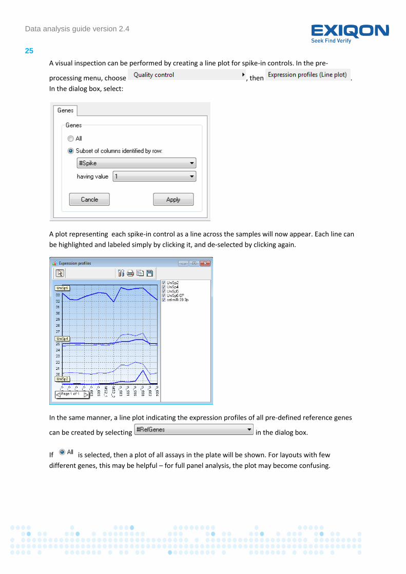
A visual inspection can be performed by creating a line plot for spike-in controls. In the pre-

processing menu, choose , then .

In the dialog box, select:

A plot representing each spike-in control as a line across the samples will now appear. Each line can

be highlighted and labeled simply by clicking it, and de-selected by clicking again.

In the same manner, a line plot indicating the expression profiles of all pre-defined reference genes

can be created by selecting in the dialog box.

If is selected, then a plot of all assays in the plate will be shown. For layouts with few

different genes, this may be helpful – for full panel analysis, the plot may become confusing.


26

Inhibited samples should be easily identified as samples deviating not only in the spike-in, but with

several other assays (e.g. reference genes), amplifying with later Cq’s (resulting from lower

amplification efficiency) than in un-inhibited samples.

The spike-in kit manual provides tables aiding in interpreting deviations in spike-in and reference

gene values, depending on sample type.

Note that not all assays will be equally affected, and thus inhibited samples cannot be rescued by

normalization. Inhibited samples should be disregarded.

Before discarding samples, please keep in mind that the spike-in is a small RNA, and thus susceptible

to RNA degrading factors such as repeated freeze-thaw cycles or presence of RNases. It is therefore

important to evaluate whether any discrepancies in Cq are due to spike-in degradation in which case

only the spike-in will deviate from other samples, or sample inhibition resulting in several assays

deviating. Apart from the line plot described above, the outlier detection described below may assist

in this task since inhibition should result in an unusually large amount of outliers, all from the

affected samples.

Hemolysis test

In serum/plasma samples, there is always a risk that hemolysis has occurred while handling the blood

samples, giving rise to cellular derived microRNA contamination. A simple way of testing for

hemolysis is by monitoring the Cq between hsa-miR-23a-3p and hsa-miR-451a. We recommend that

this Cq is used to exclude highly hemolyzed samples and to evaluate different sample sources or

sample cohorts for monitoring purposes with regards to sampling protocols and procedures.

In the pre-processing menu, choose , then .

A plot of the hsa-miR-23a-3p – hsa-miR-450a Cq is generated:


27

Any samples missing data for one of these genes will be ignored.

Samples with a Cq of less than 7 are fine, without serious indications of hemolysis. Samples with a

Cq of greater than 7 have an indication of hemolysis, and exclusion from the study could be

considered. Note that some miRs may not be affected by hemolysis, so exclusion or not should be

considered carefully.

Outlier detection

Sometimes a single well has technical problems and produces an erroneous Cq value or even a

missing value. This is the reason why we recommend running replicates. Replicates allow you to

detect and deselect a value that is an outlier. GenEx uses the Grubb’s test for this detection.

In the pre-processing menu, choose then .

In the classification column pull-down, choose your replicate classifier (either technical or biological).

Usually the default Confidence level (0.95) and cutoff SD (0.25) will be applicable, but you do have

the freedom to change these if you so desire. You can now either choose the prudent way and have

the outliers highlighted for manual inspection and deletion, or tick and have the

software automatically delete all outliers. .

Inhibited samples should light up as having many assays with outlier values (in red) compared to the

biological group. Such samples should now be removed from further analysis.

Outlier values should now be removed and not affect the averages, but should be filled in with

reasonable values for later calculations. This should be done using the Missing data handling

described below.

Negative control

A few assays may have a tendency to form primer-dimers at a lower Cq than the chosen overall cut-

off. For these assays it will be useful to set an individual cut-off based on the negative control Cq

values. GenEx is able to set such an individual cut-off in a simple operation if you have performed one

or more negative control(s), and uploaded and annotated these together with the rest of the data.

The negative controls used for this purpose may be either no template control (no RNA template

added), noRT control (no RT enzyme added in the RT reaction), or mock RT (RT reaction on carrier

RNA not containing microRNA). If your study consist of ready-to-use panels, you should run at least

one entire panel with the negative control.

NOTE: The preferred experimental design is to include at least three biological replicates or, where this

is not possible, three cDNA synthesis replicates followed by individual PCR. For more information

please go to www.exiqon.com/mirna-pcr-analysis. You may also contact Exiqon Technical Support for

help.


28

If the samples used as negative have not been defined by adding classifiers during the wizard import

(a classification column where negative control samples are identified by 1, they can easily be

identified after loading to the plate editor. Simply select the sample(s), right-click, and from the dialog

box choose and . A classification column

identifying the negative samples will appear.

To set the cut-off for affected assays, from the pre-processing menu choose

, then . In the dialog box, select the classifier

desribing your negative control samples in the pull-down menu, and the desired delta-Cq for cut-off.

In the example below, the individual cut-off will be set as the average of the negative controls for

the affected assay minus 5 Cq. Values too close to the individual cut-off will be deleted. The Negative

ctrl index indicates the value of the classifier specifying negative control samples – the default value

is 1.

If you tick , a new table will give you an overview of affected assays.

Click .

Cut off You may wish to define a cut off value indicating that data with a Cq higher than this value should be

considered background.

In the pre-processing menu, choose . In the dialog box, indicate your chosen cut-off (e.g.

37), and for now replace with a blank (just leave that cell empty).


29

Tick to remove all empty rows and undetected miRs

will be automatically removed. Partially empty rows and columns can be removed at a later step,

using the validate sheet option. Click .

Frequency of missing data Before moving on, it can be nice to get an overview of missing data. In the pre-processing menu,

choose . A new row will be added to the grid, giving the frequency

of missing data for each gene (in %).

This can be helpful in choosing parameters later, when choosing parameters for validating the sheet

(removing assays with low call rate).

Call rate plot It is often nice to get an overview of the call-rate for each assay. If you wish this to include un-

detected assays,

The plot can be generated quite simply by plotting this information. In the pre-processing menu,

choose then . Specify the cut-off

below which the expression is considered valid, whether you want only assays with less than a given %

valid values, then press .


30

The resulting plot shows call rates for each gene. The percentage of samples with Cq values below

the cut-off (valid) are depicted in green, the percentage of samples with Cq larger than cut-off are

shown in yellow, and the percentage of samples with missing values is shown in red.

Note, if you want the call-rate plot to include un-detected genes, it should be performed before

setting the cut-off and negative control.

Missing data Non-numerical values

Your real-time cycler software may have left cells empty or given values of 0 or a text (e.g.

Undetermined) in wells with no signal. These usually appear as “NAN” in GenEx and will be color

coded red. The subsequent pre-processing steps may not allow NAN values, so you need to replace

these with empty cells. The missing signal can either be due to a technical “fall-out” (no detection in

that replicate) or due to lack of expression. Fall-outs will be dealt with as outliers, so for now just

treat all as follows

In the pre-processing menu choose .

Check , leave the cell empty, and .

This will remove NaN values.


31

Assays with low call-rate

In order to make data analysis and interpretation easier, you can now remove all assays not

detected in a certain proportion of samples.

In the pre-processing menu, choose . In the dialog box, specify the percentage of

samples that should have missing values in order to render the assay undetected.

and . Be careful to set the % empty such that

assays detected in one group but not another are not removed – such assays may indeed be

important. After the message specifying which assays were removed, the window.

Note: less than x% valid data means that more than 100-x% data is invalid. I.e. if you want to

eliminate samples with more than 40% missing data, you should indicate less than 60% valid data.

Values missing due to technical issues

In the Missing Data dialog box, select and

choose the classifier identifying the type of replicas you want to use for calculating the fill-in value. If

RT replicates have been performed, this should be your first choice. If there are still missing values,

the next choice should be the biological groups.

Biological groups can be used for filling missing data by using the mean of biological groups in the

same way as mentioned above for RT replicates. An alternative method for using the biological

groups is through interpolation. When using interpolation, expression of other genes in a sample is

taken into account when calculating the value to fill in. For this method, in the Missing Data dialog

box, select .

If a subset of candidate reference genes has been created for analysis with NormFinder or geNorm

(see section on normalization), interpolation without consideration of groups can be used as a

method for filling in missing data. In this case, choose


32

microRNAs detected only in a subset of samples

In case a given miR is detected in some groups but not in others, we recommend setting the non-

detected groups to the value of the cut-off + 1. This can be done either by using the missing data

function, or manually.

In the Missing Data dialog box,, either tick

, choose the column with empty data, and

the value to fill in

or tick .

For manual fill-in, select the cells to fill in (multiple cells can be selected by holding down shift or ctrl)

and right-click. From the menu, select , fill in the dialog box

and click .

Normalization to global mean As described in the introduction of this guide, variability arising from differences in RNA samples and

handling of these samples prior to cDNA synthesis is minimized through normalization. The global

mean of all expressed genes should be the preferred method of normalization in screening studies,

where a large number of assays (>100) are analyzed without presumptions on which or how many

are regulated. It requires that the majority of tested genes have little or no regulation.

From the pre-processing menu, choose .

If you wish to normalize to global mean, simply tick .

Some genes may be expressed only in a subset of samples and filled in with above-cutoff values

during the missing data handling, while genes expressed close to the limit of detection (i.e. cut-off)

are known to have greater technical variation than genes expressed at lower Cq values. It is not

desirable to include such values in a global mean normalization. In order to avoid using such genes

for the global mean, tick , fill in the normalization cut-off of

your choice.

Before getting to normalization, you should already have considered handling of missing data – this

mainly because some downstream statistical tests require that missing data has been handled.


33

However, if you have chosen not to fill in all missing values (which in some cases may be valid), you

should click and choose the

classifier defining your groups of interest.

Click .

Normalization to reference gene(s) If the study is on a limited set of microRNAs chosen on the expectation that they should be regulated,

then global mean normalization is not an option. In this case, normalization should be to a small set

of stably expressed genes. In microRNA analysis, the preferred reference gene type would be stably

expressed microRNA, but in many cases small non-coding RNA can also be used.

Step 1: Selecting candidate reference genes

From an Exiqon miRCURY LNA™ microRNA PCR panel screening study

If a screening study using the Exiqon miRCURY LNA™ microRNA PCR panels has been performed

prior to a validation experiment, using the same sample types, then the choice of reference genes

for use in the validation study may be based upon the screening results. In this case, from the

screening study select the microRNAs most resembling the behavior of the global. These are

recognized as the microRNAs having least variation after global mean normalization.

If this method of selection is used, then 2-3 reference genes can be chosen, and it is not necessary to

further validate them since selection was based on global mean behavior during screening of the

same sample type. In that case, you can skip step 2, and continue with step 3: Normalizing to

reference genes.

From other sources

Candidate reference genes can also be chosen based on results from a different experimental

platform (e.g. microarray), from previous studies which are similar but not identical, or from

literature showing stable expression. In each of these cases, it is necessary to pick and test several

candidate reference genes (typically 5-6) and use NormFinder and/or geNorm to pick the best

reference gene(s) among the candidates.

NormFinder and geNorm both look at gene expression variance to choose the most stably expressed

genes, but they use different algorithms to do so and may come up with slightly different results. It

may be useful to perform both analyses, and then select reference genes they agree on.

Step 2: Choosing reference genes from candidates using NormFinder and/or geNorm

Before performing the NormFinder and/or geNorm analysis, you need to identify the candidate

reference genes in your experiment in a manner that GenEx understands. For the full panels, Exiqon

has already made a suggestion for candidate reference genes, and these were automatically

classified as such. It may be desirable to add further candidates before proceeding with choosing the


34

optimal genes. For Pick&Mix, candidate reference genes may have been identified during the plate

configuration. If they were not, you can specify the candidate reference genes to GenEx now.

To specify candidate reference genes, simply select the columns containing candidate reference

genes, (multi-gene selection is possible using shift or ctrl). Right-click and from the menu, choose

, then .

Once reference genes have been classified, a classification row will appear at the bottom of the Data

editor table identifying candidate reference genes by a 1.

Now create a data subset containing only the candidate reference genes. In the menu,

choose then . The subset will open in a new data editor.

the subset to the Control panel to perform NormFinder and/or geNorm analysis.

The following example illustrates how to select reference genes after creating a subset of the data

from the panel.

In the main window, there is a ref gene tab. Make sure that this is the active tab.


35

You can perform both NormFinder and geNorm analysis on the reference gene data. For NormFinder,

you have the added option of looking at intergroup variation – i.e. whether assay variation is stable

across groups and not just across samples.

NormFinder:

Click , verify that Plot SD and View Acc. SD are ticked to get graphs of standard deviation and

accumulated standard deviation, respectively.

then .

You should get an output consisting of 3 windows, similar to this:

geNorm:


36

Click . is ticked by default and should not be

changed. Click .

You should get an output consisting of 2 windows, similar to this:

Selecting the reference genes

Both algorithms provide you with a table of values indicating the variability of each gene (M-value in

geNorm, SD in NormFinder) and the best gene and/or best gene combination.

Both algorithms provide bar-charts showing which genes are most stably expressed (most stable

gene to the left). Keep in mind that these are two different algorithms, so they may not always come

up with the same answer. However, combined they should give a good indication of which genes are

most stably expressed and which are less so. In this example, we would not choose U6 as a reference

gene.

Normfinder provides an additional graph of the accumulated SD, indicating in red the optimal

number of reference genes, which may be from 1 to more than 5 (in this case 2, i.e. SNORD38B and

SNORD49A).

Choosing the best reference genes now becomes an educated estimate – there is no final solution.

geNorm selects the top pair of the most stably expressed reference genes, in this example hsa-miR-

423-5p and hsa-miR-103, and tells us that all candidates except U6 could be good choices.


37

NormFinder indicates that 2 reference genes might be optimal, and that all candidates except U6

could be good choices. The option therefore could be to choose all but U6 as a set of 5 reference

genes – or, to just choose the 3 stable microRNAs. But do keep in mind: more is not always better.

Step 3: Normalizing to reference genes

Once the final choice of reference genes has been made from the candidate reference gene subset,

the candidate reference genes not used for normalization should be changed back to 0 in the

original data editor containing the full data set. To do so, activate the edit button and simply

edit the classifier value(s).

Now you are ready to perform the normalization.

In the pre-processing menu, choose . In the dialog box,

activate , select and set . Now click

. The pane should now be filled in to indicate the chosen

reference genes

Click

Average RT replicates As recommended earlier, the reason for including replicate RT reactions is to get more robust data

with the option of omitting potential outliers due to technical issues. But, in the end, we are

NOTE: In the “delta delta Cq” calculation, this step is the first delta Cq


38

interested in comparing just one value for each sample. This value is obtained by averaging the

accepted technical replicates.

In the pre-processing menu, select .

In the Normalize by column pull-down select your replicate classifier and .

You will notice that the replicate rows have disappeared, leaving one row for each sample. These

now contain the average of the replicates, after removal of the outliers.

Converting to relative quantities The numbers in the data table by now will not resemble the original Cq values. However, they will

still be on the logarithmic scale of Cq values. It is therefore helpful to convert these values to relative

quantities on the linear scale.

Step 1: Relative quantities

In the pre-processing menu select .

You now have several options for how you want values to be related:

What you want your data relative to depends on the study design and the output wished for. It may

make sense to do relative to a control group – or in some cases relative to nothing (this gives nicer

scatter plots).

NOTE: The data have now been converted to linear scale according to the following formula:

N =2(Cqrel-Cq)

where Cqrel is the Cq value you are relating to (i.e. normal, untreated, or average).


39

Step 2: Log conversion

Many statistical tests, such as T-test and ANOVA, assume normal distribution. This is not always a

true assumption when working with expression data at the linear scale, but by converting to log

scale normal distribution is often obtained. Furthermore, some graphical representations are easier

to view in the log scale.

In the pre-processing menu you choose . Of you prefer a different log base, more options

are available by choosing .

Click , and in the dialog box click yes for saving your data. Choose a path and file-name,

and .

Your data has now been pre-processed and is ready for analysis by the multiple statistical features

provided by GenEx.


40

Further data analysis using GenEx After pre-processing is completed, you can either continue directly with analysis of the loaded data,

or get back to this later. If you continue at a later time, you should import the pre-processed data set

(saved at the end of pre-processing) using the load file function . You should now have a

project in the data manager, containing your pre-processed data set and log of pre-processing steps

performed

At any time during data analysis, you can save your project with all analyses performed using the

export project function . You can then get back to the project at a later time by importing the

projet to the control panels .

If at some point you have too many windows open, you can close everything but the Control panel

by clicking . An already performed test can be re-performed by cliciking it in the tab of

the Control panel.


41

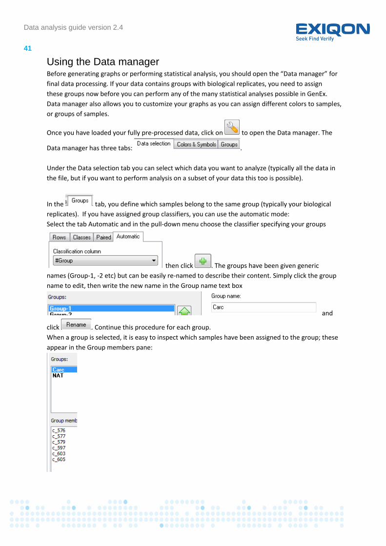
Using the Data manager Before generating graphs or performing statistical analysis, you should open the “Data manager” for

final data processing. If your data contains groups with biological replicates, you need to assign

these groups now before you can perform any of the many statistical analyses possible in GenEx.

Data manager also allows you to customize your graphs as you can assign different colors to samples,

or groups of samples.

Once you have loaded your fully pre-processed data, click on to open the Data manager. The

Data manager has three tabs: .

Under the Data selection tab you can select which data you want to analyze (typically all the data in

the file, but if you want to perform analysis on a subset of your data this too is possible).

In the tab, you define which samples belong to the same group (typically your biological

replicates). If you have assigned group classifiers, you can use the automatic mode:

Select the tab Automatic and in the pull-down menu choose the classifier specifying your groups

then click . The groups have been given generic

names (Group-1, -2 etc) but can be easily re-named to describe their content. Simply click the group

name to edit, then write the new name in the Group name text box

and

click . Continue this procedure for each group.

When a group is selected, it is easy to inspect which samples have been assigned to the group; these

appear in the Group members pane:


42

In the tab, you can choose the color of each sample or group for bar charts and the

symbol for each sample or group for graphs such as PCA plots.

Tick , select each group in turn and assign colour and/or symol

to the group.

When you are finished remember to click .

Statistical analysis in GenEx GenEx offers a wide range of statistical analyses (some of which require specific experimental

designs). In the Statistics tab you can choose from different analyses. We recommend as a minimum

performing either a T-test (in case of only two groups) or an ANOVA (if multiple groups are tested):

T-test compares two groups of data, where the group selected as B is considered the control,

and A the group with changes.

The will give a list of the tested assays, sorted by P value (statistical

significance). It will also specify whether a normality test was performed and passed, the linear fold-

change between groups, and the difference between the two groups on a log scale. If the P-value is

significant even with Bonferroni correction, the P value is green. If significance is obtained by

ignoring Bonferroni correction, the P value is yellow. If the difference is not statistically significant,

the P value will be in red. Below is shown an example in the P-Value compact view, without

advanced multiple testing.


43

In addition, you can choose advanced multiple testings, or a graphical representation in a volcano

plot by ticking these options in the t-test dialog box before pressing run.

A one-way ANOVA tests for differences between groups considering one parameter (e.g.

different treatments).

In a one-way ANOVA a P-value for significance of difference between groups as well as various

statistical test values will be given for each gene.


44

In addition, a list of P values of difference between groups will be created, similar to the result for a

t-test.

In a two-way ANOVA, testing for two different parameters (e.g. genotype and time) is possible.

A table showing the result for each tested microRNA will result.

The result of a two-way ANOVA indicates the significance of each factor, as well as the interaction of

the two (i.e. whether the two factors influence each other).

Creating a subset of regulated assays When working with full panels, the figures created by e.g. Descriptive Statistics or Heat-map may

become difficult to interpret due to the very large number of assays involved. In such a case, it can

be useful to create a subset of assays including only those assays of interest (e.g. only regulated

assays).

A subset of assays regulated between two groups can be created either from a t-test or a Scatter

plot.

Subset from t-test or one-way ANOVA

If a t-test or one-way ANOVA has been performed, select the assays of interest (based on P value

and/or difference) while holding down shift or ctrl.


45

Then click , and . Name your subset.

In the t-test, you can also create your subset from the volcano plot if that option was ticked when

running the test.

In the volcano plot window, tick , and a list of regulated genes is shown in the right-hand

pane. The list is based on the fold-change sliders (the vertical lines), which can be moved simply by

click-and-drag. By default, genes with statistical significance changes are pre-selected, with the

option of selecting further genes by ticking them. Once you have selected the genes you wish in the

subset, click Create group of Genes. Name your subset.


46

Subset from Scatter plot

A scatter plot can be made in the Correlation tab, by clicking . In the dialog box, choose Groups

of samples, and the two groups to plot. Check Show significance area, Distance from center (1

corresponds to a 2-fold regulation if the data is log2 transformed), and List genes outside area.

Check and

Click


47

Note that if you have chosen one group relative to the other when you set relative values during pre-

processing, then by the very nature all values in the group relative to have been set to 0 – and thus all

values will lie on a straight line. This is not an error, just a result of valid data manipulation.

In the table grid, select the genes you wish to include in the subset and create the subset in the

same way as for the t-test. Name the subset.

Activating only the subset genes

In the main window click to open the data manager. In the Data selection tab, Columns sub-

tab click then . All assays will now be de-activated. Now, in the

selection box choose the group you have created, click and . More than

one subset can be activated in the same round, by selecting the next group and activating that

selection. Activated genes can be recognized by having a next to them in the list, while de-

activated genes are recognized by having a next to them. Press and .

Note that you have now de-activated all genes currently not of interest. Nothing has been deleted –

these genes can always be activated again at a later time.


48

Furthermore, several very nice graphical representations of the data set can be selected. If a large

number of genes have been tested (e.g. full miRNome), it is recommended to create a subset of

microRNAs of interest before creating the various graphical presentation.

Descriptive Statistics gives a graphical representation of expression differences, with error

bars as Standard deviation (STDEV), Standard error of the mean (SEM) or Confidence Intervals (CI)

according to preference.

Principal component analysis shows how the samples group together. If colors have previously

been assigned by grouping, it becomes easy to see whether the samples group as expected.


49

Heat-map shows clustering, depicting grouping of microRNAs and samples


50

To find out more about these and other statistical analysis options, please see the GenEx Help

function.

Many other types of plots and analysis possibilities are available, such as non-parametric statistical

tests, Cohonen self-organizing maps, and nested ANOVA. The GenEx help function contains detailed

explanations for these types of analyses


51

Gene info GenEx can easily retrieve microRNA information on the assays used in and experiment from a

number of relevant databases such as miRBase, miRecords and miRTarget (among others). You can

also directly retrieve information on available probes from Exiqon’s webshop, to ease the way into

functional analysis.

Once the project has been loaded to the control panel, click in the software toolbar menu.

Then select your assay of interest in the dialog box appearing, choose the database of interest from

the pull-down menu and click search.

GenEx will now start your internet browser, and find the selected microRNA in the chosen database.


52

Quick steps for experienced users Import data using wizard

Remember classifiers – minimum #Group

Interplate calibration

Quality control

o Internal amplification control outliers

o Expresssion profiles

candidate reference genes

spike-ins

o Serum/plasma: Hemolysis test

o Outlier detection

o Negative control

Cut off

Frequency of missing data

Call rate plot

Missing data – non-numerical values

Validate sheet: Assays with low call-rate

Fill in missing data based on

o Technical replicates

o Groups

o Specified Cq for non-detected groups (Cut-off +1)

Normalization to global mean or ref genes

Average RT replicates

Convert to relative quantities + Log2

Load

Define groups from classifiers


53

Online help

For technical support please go to:

http://www.exiqon.com/contact

Join the GenEx online forum where you can ask other users and experts about qPCR data analysis

and GenEx, please go to:

http://www.multid.se/forum.php

References

1. A novel and universal method for microRNA RT-qPCR data normalization.

Mestdagh P, Van Vlierberghe P, De Weer A, Muth D, Westermann F, Speleman F, Vandesompele J.

Genome Biol. 2009;10(6): R64

2. Normalization of microRNA expression levels in quantitative RT-PCR assays:

identification of suitable reference RNA targets in normal and cancerous human solid tissues.

Peltier HJ, Latham GJ.RNA. 2008 14(5): 844-852

3. Identification of suitable endogenous control genes for microRNA gene expression

analysis in human breast cancer.

Davoren PA, McNeill RE, Lowery AJ, Kerin MJ, Miller N. BMC Mol Biol. 2008 9: 76.

http://www.exiqon.com/contact

http://www.multid.se/forum.php

Documents

Data Analysis Guide - TATAA Biocenter · This data analysis guide will provide an instruction on how to export data from the most common ... For ABI Viia 7, 7900, ... PCR Instruction