Overview of data collection, management and processing procedures

of underway acoustic data - IMOS BASOOP sub-facility.

Author: Tim Ryan

Version 1.0

2nd May 2011

Overview The IMOS Bio-Acoustic Ship Of Opportunity (BASOOP) sub-facility commenced on the 1st of July 2010

to collect underway acoustic data while vessels are transiting ocean basins (Figure 1). The primary

data-type recorded from the vessel-mounted echosounder systems is georeferenced calibrated

water column volume backscatter, Sv [dB re 1 m-1], (Maclennan et al. 2002) . Data acquisition

protocols that optimise the quality and utility of the acoustic data have been devised and

communicated to the participating vessels (Appendix A). The raw acoustic data is post processed to

(i) identify on-transit data and prioritise processing, (ii) apply calibration offsets, (iii) apply semi-

automated filters to identify and reject bad data and (iv) output and stored in netCDF format, mean

echointegrated volume backscatter sv (in linear units [m-1]) Sv for cells of 1000 m distance and 10 m

height. A full metadata record is also stored in each netCDF file. The document SOOP-BA NetCDF

manual v1.0.doc describes the netCDF format and metadata fields that have been defined.

Figure 1. Image of basin-scale acoustic backscatter Sv data for a transit from Australia to New Zealand by FV Rehua in August 2010. Screen gain set to -78 dB. Black regions are where data from the seafloor and below have been excluded. Vertical grid lines indicate 100 km distance, horizontal grid lines indicate 100 m depth intervals down to a maximum depth of 1200 m.

At present, nine vessels are participating in the BASOOP program. Six are commercial fishing vessels

that have agreed to record data during transits to and from fishing grounds. The remaining three

are scientific research vessels collecting underway acoustic data during transits and science

operations (Table 1). All vessels collect 38 kHz acoustic data from either Simrad EK60, ES60 or ES70

echosounders. In all cases the 38 kHz echosounders are connected to Simrad ES38B transducers.

This is a narrow-beam (7 °) ceramic transducer with good long term stability and manufacturer

supplied calibration parameters. Research vessel Southern Surveyor also collects concurrent acoustic

data at 12 and 120 kHz. The research vessel Aurora Australis collects concurrent acoustic data at 12,

120 and 200 kHz.

Table 1. Table of participating vessels

Vessel Name Simrad Acoustic transceiver(s)

Acoustic transducer(s)

Institute/Company Key transits

RV Aurora Australis 38 kHz EK60 120 kHz EK60 12 kHz EK60 200 kHz EK60

ES38B ES120-7 EDO323HP ES200-7

Australian Antarctic Division

Hobart-Antarctic transits.

RV Southern Surveyor

38 kHz EK60 120 kHz EK60 12 kHz EK60

ES38B ES120_7C 12-16/60

Marine National Facility

Australian EEZ, occasional trips to Pacific

RV L’Astrolabe 38 kHz ES60 ES38B IPEV (France) Hobart-Antarctic transits.

FV Rehua 38 kHz ES60 ES38B Sealord NZ Aust-NZ transits, NZ EEZ, Tas west coast

FV Janas 38 kHz ES60 ES38B Sealord NZ NZ – Ross sea

FV Antarctic Chiefton

38 kHz ES60 ES38B Sealord NZ Mauritius - Heard McDonald Islands

FV Southern Champion

38 kHz ES60 ES38B Austral Fisheries Pty Ltd

Mauritius - Heard McDonald Islands

FV Austral Leader II 38 kHz ES60 ES38B Austral Fisheries Pty Ltd

Mauritius - Heard McDonald Islands

FV Saxon Onward 38 kHz ES60 ES38B Onward fishing Pty Ltd South-east fishery

Data collection procedures Data collection procedures have been developed for each of the participating vessels. They have

been devised to optimise the quality and utility of the collected data while considering the

operational needs of the vessels (Table 2). Appendix A gives an example of a current working

document for collecting data from commercial vessels.

Table 2. Basic data collection settings

Parameter 38 kHz 12 kHz 120 kHz 200 kHz

Power (W) 2000 Check 500 120

Pulse length (ms) 2.048 1.024 1.024 1.024

Logging range (m) 0-2000 0-2000 0-500 0-500

Absorption (dB/m) 0.0097853

Sound speed (m/s) 1493.89

Vessel calibration

Vessels are calibrated according to the procedures recommended in the ICES CRR 144 document by

(Foote 1987). In the case of ES60 systems, the calibration data is pre-processed to eliminate the

possibility of bias of up to +/- 0.5 dB due to the systematic triangle wave error that is embedded in

the ES60 data (Ryan and Kloser 2004). This triangle wave error can be significant for calibration data,

but for field data it averages to zero over long periods and is not considered a significant source of

error. Hence processing to eliminate the triangle wave error from field data is not done.

At a minimum vessels will ideally be calibrated annually but logistics may dictate different time

intervals. Table 3 shows the current calibration status of each of the participating vessels along with

the expected date of the next calibration.

Table 3. Calibration status of participating vessels.

Vessel Company or Institute

Last Calibration

Expected date of next calibration

Expected location

Normally carried out by:

Comments

Aurora Australis

AAD approx 5 yrs ago

Oct-2011 Hobart CSIRO In discussion with AAD to obtain allocation of time from AAD logistics.

Southern Surveyor

National Facility

Oct-2009 Apr-11 Hobart CSIRO In voyage schedule for March 2011

L'Astrolabe IPEV Never Summer 2011

Hobart CSIRO In discussion with IPEV to find mutually suitable time.

Rehua Sealord Sep-2010 Jun-2011 Nelson NZ

NIWA Regular calibration as part of Tasmanian west coast blue grenadier survey work.

Janas Sealord Jul-2009 TBA NZ NIWA Janas has been calibrated previously by NIWA. Not known if this will continue. Discuss with Graham Patchell (Sealord) and/or NIWA - Richard O Driscoll

Will Watch Sealord Unsure TBA Mauritus FRS South Africa

Possibly calibrated in 2007 as part of SIODFA, high seas fisheries project

Antarctic Chiefton

Sealord Unsure TBA Mauritus FRS South Africa

Possibly calibrated in 2007 as part of SIODFA, high seas fisheries project

Austral Leader II

Austral Fisheries

Dec-2009 TBA Mauritus FRS South Africa

In discussion with Austral Fisheries to establish time/place of calibration

Southern Champion

Austral Fisheries

Dec-2009 TBA Mauritus FRS South Africa

In discussion with Austral Fisheries to establish time/place of calibration

Saxon Onward

Onwards fishing

Jun-2010 Jun-2011 Hobart CSIRO Calibrated in 2010 as part of CSIRO project and expect to be done in June 2011

Data management procedures In-house tools have been developed to assist with data management and help identify and prioritise

subsets of data for post-processing. The data management tool borrows from the open-source

multi-beam processing software MB-System (http://grass.osgeo.org/wiki/MB-System) approach by

generating from each of the acoustic raw files, a corresponding inf file. The inf file is in text format

and contains the temporal and geographic extent of the associated raw file. The inf files are created

during a data registration process using the tool ES60_register.jar. User defined metadata can be

included during the registration process (e.g voyage name, vessel name). During registration

metadata can be automatically extracted from the binary raw files and included in the inf file (e.g.

Echo sounder serial number).

The inf files can be visualised as geo-referenced rectangle blocks using our open-source software

Dataview.jar (Figure 2). Dataview.jar has the tools to select blocks of inf files by defining time-

windows, spatial extents, and keywords or a combination of these.

Figure 2. Visualisation of inf files generated during a registration process of a set of corresponding acoustic files

Structure of data storage area

1. Raw data

\\Rawdata\VesselName\\VesselName_StartDateOfVolume_EndDateOfVolume

2. Processed data

\\Processeddata\VesselName\\VesselName_StartDateOfVolume_EndDateOfVolume\\

3. Pending registration

\\Pending_registration\VesselName

Data processing procedures Data processing for the SOOP-BA data follows the flow chart shown in Figure 3. Terms and

definitions used in the text are given in Table 4.

Table 4 Terms and definitions

Term Description

Sv Acoustic volume backscatter in dB re 1m-1

(Maclennan et al. 2002)

Echogram pixel-level Sv values produced either by the echosounder at the time

of acquisition or by post-processing software.

Sv.ESdata Electronic file containing echogram-level data. Examples include Simrad

raw and HAC formats (ICES 2005).

Mean acoustic volume backscatter obtained through echointegration of

calibrated but non quality checked data.

Mean acoustic volume backscatter obtained through echointegration of

calibrated and quality checked data.

A “cell” of data will span an interval based on either distance travelled,

elapsed time or number of pings and will exist at a defined range from the

transducer. The associated coordinate variables are time, latitude and longitude

for the horizontal echointegration interval, and range to define the cell-

transducer distance. The standard output for the SOOP-BA data is a cell of 1000

m distance and 10 m height. This metadata standard will define the format of

and the corresponding coordinate variables as well as detailing required

ancillary variables.

Electronic file containing echointegration data that is generated by the post

processing software.

Electronic file containing echointegration data generated by the post

processing software and metadata as defined in this document. Units are linear,

m-1

.

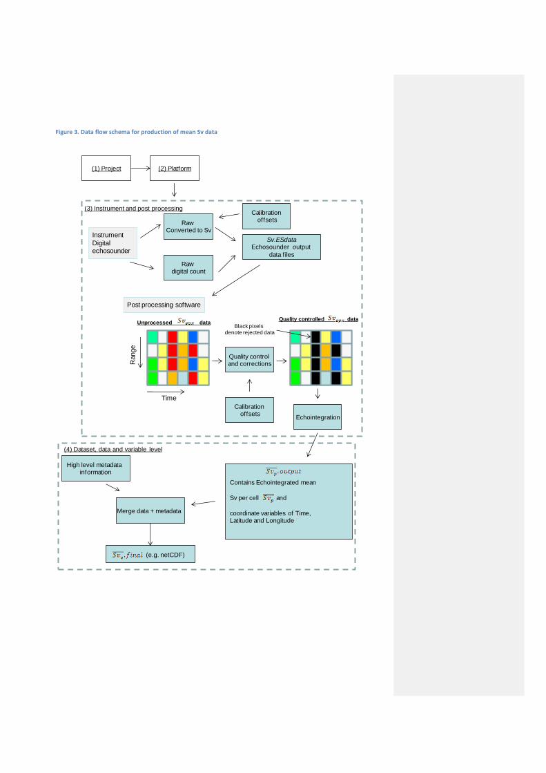
Figure 3. Data flow schema for production of mean Sv data

Raw digital count

Instrument

Digital echosounder

Raw Converted to Sv

Sv.ESdataEchosounder output

data files

(2) Platform(1) Project

Post processing software

Time

Range

Quality control and corrections

Echointegration

Calibrationoffsets

Calibrationoffsets

Black pixels denote rejected data

Unprocessed dataQuality controlled data

Contains Echointegrated mean

Sv per cell and

coordinate variables of Time, Latitude and Longitude

(e.g. netCDF)

High level metadata information

Merge data + metadata

(3) Instrument and post processing

(4) Dataset, data and variable level

Data processing is carried out via the following steps:

Generate a list of on-transit acoustic files to process using Dataview’s visualisation of inf

files.

Using Myriax’s Echoview software controlled by a Matlab script via COM objects:

o Create Echoview ev files using an ev template for manageable blocks for raw

acoustic data (nominally a new ev file is created for each 6 hours of raw acoustic

data). Note the ev template will have been set up to contain data quality filters and

to have the appropriate calibration parameters.

o Processing to identify and eliminate bad data. In order to calculate both a correct

mean Sv and area backscatter (NASC) for the echointegration cell, rejected sample

values need to be set to either ‘no data’ or -999 dB depending on which criteria led

to the value being rejected (Table 5).

Table 5. Rejected data values set according to filter criteria

Filter criteria Value Comment

Spike No data Elevated signal for a portion of a ping

Attenuated ping No data Set ‘whole excluded or no-data pings do not reduce the

thickness mean’ to yes

Below threshold

values

-999 dB Signal is below detection limit of echosounder, set values to

zero (i.e. -999 dB)

Below seafloor No data Set ‘exclude below line’ where line is the ‘acoustic bottom’

Echo integrate and output to csv format. Note, echo integration is executed on three

different data types. Firstly for the original unfiltered data, secondly for the quality

controlled filtered data and finally an output to quantify the number of retained (i.e.

unfiltered) samples. The quality controlled filtered Sv values are the ones that

should be used as the blessed data. The ratio of retained quality controlled data to

original data is used to give a metric of data quality. Similarly, comparisons can be

made between filtered and unfiltered Sv values as an indicator of data quality. Data

quality is likely to be high where there is little or no difference between filtered and

unfiltered Sv values. Conversely where there is a large difference, the data quality is

likely to be lower.

Note: Echoview processing uses nominal absorption and sound speed values as per

Table 2. Absorption and sound speed values were calculated using the equations of

(Francois and Garrison 1982) and (Mackenzie 1981) respectively. Secondary

corrections to account for changes in absorption and sound speed due to temporal

and geographic related changes in water temperature and salinity may be made to

the Sv values in the output netCDF file if required. Range-dependant changes to the

cumulative absorption and sound speed also may require a secondary correction to

be applied. Similarly, temperature related changes in calibration sensitivity (Demer

and Renfree 2008) may require secondary corrections to the Sv values in the output

netCDF file.

Convert echo integration csv format data to IMOS Netcdf format, merging in all necessary

metadata at the same time. The document SOOP-BA NetCDF manual v1.0.doc details the

metadata standard associated with the SOOP-BA data.

Processing to identify and eliminate bad data

We define two types of noise. Background noise is generally at a consistent value for many pings,

but as a minimum is constant throughout the duration of one ping. Intermittent noise consists of

signal from unwanted sources that is only present for a portion of a ping. Intermittent noise may

only exist for a moment (i.e. at a certain range) within one ping, but may persist across multiple

pings at a similar range.

Referring to Figure 3, the processing steps associated with the ‘Quality control and corrections’ stage

contain four sequential filter stages: i) simple intermittent ‘spike’, ii) attenuated signal, iii) persistent

intermittent noise and iv) background noise.

Simple intermittent noise spike filter

A typical intermittent noise ‘spike’ is interference from another echosounder. This type of

interference adds unwanted signal momentarily at a range and persists only for 1 ping. This filter is

based upon the one described in the paper by Anderson et al. (2005)

Procedure: Echograms are time shifted by n and n*2 pings (usually n = 1) then a comparison is made

to check for instances where Sv values rise and fall by an amount above a defined threshold.

Data is resampled into cells of 20 m height and 1 ping width to reduce the vertical resolution and

so reduce within ping pixel-pixel variability. The resampling algorithm outputs the median values

within the resampling cell.

The resampled data is then time shifted by -1 and -2 pings to create two new echogram

variables.

A formula operator is used to compare between echograms that have been shifted by 0, -1 and -

2 pings according to the following equation:

That pixels are rejcted if the centre pixels (V1) are greater than the proceeding (V2) and

subsequent (V3) pixels by 10 dB and is greater than -80 dB. The -80 dB threshold is set to avoid

the high degree of variability that often occurs in low signal region registering as a spike.

Referring to Figure 4, according to the formula the red line is classified as a spike. The green line

doesn’t qualify as it persists for more than one ping. The blue line doesn’t qualify as it doesn’t

exceed the 10 dB threshold.

Figure 4. Example of noise spike

Attenuated signal filter

This filter is used to identify and eliminate pings whose signal has been attenuated by an amount

exceeding a user defined threshold. In bad weather vessel-wave interactions can generate micro-

bubbles which may highly attenuate the acoustic signal. In such situations the acoustic signal will be

attenuated by the same amount throughout the duration of a ping. Further, successive pings may be

attenuated for extended periods until the water beneath the vessel becomes clear of micro-bubbles.

Procedure: This filter follows the Simple Intermittent Noise Spike. It assumes that there are

reasonable (but not necessarily perfect) levels of localised homogeneity in the deep scattering layer

(DSL, 300-600 metres depending on time of day). Pings whose signal is less than the median localised

value of the DSL by a user define amount can be identified as being attenuated. An attempt to

automatically detect the DSL is made but usually requires some editing the manually define a line

that takes in the high scatter region that constitutes the DSL. Precise effort here is not required, so

long as a region with reasonable homogeneity and signal-to-noise is defined. The processing steps

are:

Bitmap operators are used to mask an echogram region defined by the defined upper DSL line

and the lower DSL line (upper DSL line + 100 m).

The Sv data within the masked DSL region is resampled in two ways to produce two new virtual

variables.

o Firstly, for each ping, the data in the defined DSL region is resampled at a width of 1 ping

and a single value of the 25th percentile of the DSL data for each ping.

o Secondly, the DSL is resampled to give a single Median value within a resampling

window of n pings.

Using a match ping times operator virtual variable of the median resampled data is generated to

have the same ping geometry as the per-ping lower percentile resampled data. This allows a

comparison to be made between the per-ping lower 25th percentile value within the DSL region

and the median value over n pings. If the per-ping value is less than the localised median value

by a defined amount, then the data is considered to be attenuated. Unlike transient spike data,

this type of attenuated data affects the entire ping. Therefore the entire ping is marked bad. The

formula used is:

-75

-70

-65

-60

-55

-50

1 2 3 4 5 6 7 Not a spike

Spike

Not a spike (2)

Where V1 is the median value over N pings and V2 the per-ping lower 25th

percentile.

Comments: The value chosen for n pings for the median resample is a compromise. Too many pings

may mean that comparison between the resampled Median value and the per-ping resampled lower

percentile value is no longer a robust indicator of signal attenuation. If n is small, attenuated pings

that persist for multiple pings regions may not be identified. Our processing to date has used values

between n = 30 and n=300 following inspection the echograms and reviewing the effectiveness of

the attenuation filter.

Persistent intermittent noise

Procedure: This filter follows the Simple Intermittent Noise Spike Filter and the Attenuated signal

filter. The Simple Intermittent Noise Spike Filter is very effective for spikes that are only 1 ping wide.

However in bad weather intermittent noise may persist over multiple pings requiring a different

approach to be taken. This filter stage is a more robust solution that will eliminate elevated signal

when compared to median values within a localised resampled region. This filter works in a similar,

but not identical, way to the Attenuated signal filter.

Input data is converted to 40 Log R TVG. This has the effect of overemphasising the

signal as a function of range, so highlights the spike noise at deeper depths where they

tend to be more problematic.

40 Log R data are resampled to give the lower percentile (nominal value 15th percentile)

for cells of n pings wide (nominal value n=50) and height of 10 metres over the entire

echogram range. These samples will give a measure that can be used as a benchmark to

compare ping-by-ping deviations from the localised resampled values.

The lower percentile resampled values are subtracted from the 40 log R data.

Intermittent noise data will deviate from the lower percentile resampled values by a

greater amount than clean data.

A formula operator is used to identify original data samples that deviate from the lower

percentile resampled data by +/- a defined amount according to the formula:

Where V1 is equal to 40LogR Data – lower percentile resampled data and V2 is the

original data. Values below a defined threshold (-70dB) are ignored in order to avoid

rejection of highly variable low signal samples. V3 is a user-defined surface region

where data will always be good: This filter will ‘erode’ small high signal regions such

as small schools. Such regions are typically observed in the upper water column

regions and conversely, where noise spikes are generally less of a problem. To avoid

this, the upper region of the echogram (usually ranges less than 300m) is masked as

always true to avoid inadvertent rejection of valid signal.

Comments: the size of n for the median resample is a tradeoff. It needs to be large enough to

capture a persistent series of spikes over a number of pings but small enough to avoid identifying

small school regions (which also appear as elevated signal) . The default of N=50 seems to be a

reasonable tradeoff, but this can be adjusted empirically depending on the nature of the water

column signal. Masking off the surface layer from the effects of this filter goes long way towards

preserving legitimate school information while proving effective in taking out persistent spike noise

regions at deeper ranges.

Background noise

The final stage in our processing is to remove background noise using the method described by (De

Robertis and Higginbottom 2007). A key assumption with this method is that a noise-only region

exists in the data (in practice at the longest range of the echogram). That is, spreading losses have

reduced the return signal to insignificant levels compared to the constant background noise. For this

to be the case, the echogram range needs to extend well into this ‘noise only’ region. Some of the

SOOP-BA data has been collected to shorter ranges and will not provide a ‘noise only’ region. In

those instances the Background Noise filter cannot be used in the processing. Note, we now specify

a data acquisition range that will include a noise only region (a maximum range of 1800 metres will

achieve this for the vessels that currently are participating).

Metrics of data quality

Two metrics that can be used as indicators of data quality are provided as ancillary variables to

accompany the values. These are:

i) The percentage of data rejected (denoted as Sv_pcnt_good_<id> in the SOOP-BA netCDF

manual, where <id> indicates the frequency). This is derived from the ratio of the

number of pixels in the cell to the number of pixels in the cell.

ii) The mean echointegration value of non quality checked data, , denoted as

Sv_unfilt_<id> in the SOOP-BA netCDF manual, where <id> indicates the frequency.

Cells of where the percentage of rejected data is greater than 50% are automatically marked as

no-data (-999) values in the file. Further work is being done to develop guidelines to help

inform users regarding data quality and will be communicated in an updated version of this

document.

Appendix A. Open Ocean Data Logging

Simrad ES60 Open-ocean data logging

Version 1.3

May, 2010

Simrad ES60 Open-ocean data logging

This set of instructions describes how to set up the Simrad ES60 38 kHz echosounder to record data

when on the open-ocean.

System requirements

Simrad ES60 running software versions 1.4.xx or higher

USB external hard drive

Keyboard with Windows button (only very old keyboards would not have this key)

Mouse attached to ES60 PC

System settings

- Set data to log to a folder on the external USB hard drive - Set Power 2000W; Pulse length 2.048 ms - Set display range 0-2000 m - Set bottom detection range from 1999 to 2000 m - Set ES60 PC clock to UTC and reset against GPS time source - Log data from port to port

If you are unsure how on any of these settings, details on how to set them up are given below in

steps 1-6.

A word of thanks ….

The areas that fishing vessels work in, and the transits to get there, give a unique opportunity to

collect data from areas that cannot be accessed by research vessels on a regular basis. The

information collected is forming part of a valuable data set that is helping us to better understand

the ocean environment.

Thank you for taking the time to record this data.

1. Set logging directory

On the very top LHS of the ES60 screen click File/Store and then the Browse button to navigate to

the externally attached hard drive and select a suitable folder for the logged data. Set the file size to

25 MB and uncheck the box that says “Local time”

Tip. USB drive letter will not be C and is unlikely to be D, and is probably E on most installations.

Supplied drives will most likely have a folder \Data. If so log to this folder: That is: E:\Data.

Tip. If you need to set up a logging directory, hold down the Windows button on the keyboard (

) and press E. This will bring up Windows Explorer. You can then find your way to the

USB hard drive and create a folder to log to.

Tip. Hold down the alt-key and press the Tab button. This will take you back to the ES60

software.

D:\data E:\Data

25

1

D:\data E:\Data

25

1

2. Set Echosounder power and pulse length

On the top of the ES60 screen right click on the text “38 kHz” to bring up the transceiver settings

dialog. Set the power to 2000 W and the pulse length to 2.048 ms and click OK

2000

2.048

Right click here

2000

2.048

2000

2.048

Right click here

3. Set display range

Once the vessel has got to deep water (say > 500 m) set the display range from 0-2000 metres by

right clicking on the RHS of the ES60 screen.

Right click hereRight click hereRight click here

2000

4. Set logging range

We need to log down to 2000 metres. This can be compromised if the sounder locks onto false

bottoms in the water column which can happen when the vessel is in open ocean. To avoid this right

click on the depth value in the top-middle of the ES60 screen. Set the bottom detection start to 1999

meters and finish at 2000 metres. Note that in this mode the depth value will always be 0 metres

which is not a problem for open-ocean logging but if this reading is needed for navigational purposes

the depth setting should be reset.

5. Set the ES60 PC clock to UTC

Hold the windows button ( ) and press M to get to the ES60 PC’s desktop.

At the bottom RHS of the screen double click on the time readout to bring up the Date/Time dialog.

Right click hereRight click here

2000 1999

Comment [klo010 1]: Is this right – I thought it was 1500 m? are we getting good performance of the systems to 2000 m

Click on the TimeZone tab. Select GMT from the pick list and click OK.

Click on the Date&Time tab. Reset the time to match the UTC time from a GPS readout.

6. Commence logging Alt-tab back to the ES60 software. At the bottom RHS click on the text “L000..”. This should turn

from black to red to indicate logging has commenced.

Turn off other sounders when logging in open ocean to avoid unwanted interference

Tip Log from port to port. This avoids the risk of forgetting to turn logging on when reaching

deep water.

7. Reverting back to non-open ocean settings

When in waters less than 2000 meters and fishing is commencing you can set the bottom detection

back to 4 to 2000 meters so that meaningful depth is output. When fishing if depths are less than

700 meters you could choose to set the pulse length to 1.024 ms to give a higher resolution image.

Leave the Power at 2000 W at all times as this is optimal for both fishing and scientific work.

Contact details If you have any problems please don’t hesitate to contact me.

Tim Ryan

Mobile: +61 (0)408 591 048 (Australia)

tim.ryan@csiro.au

Work +61 (0)3 62325 291

References Anderson, C.I.H., Brierley, A.S., and Armstrong, F. 2005. Spatio-temporal variability in the distribution of epi-and meso-pelagic acoustic backscatter in the Irminger Sea, North Atlantic, with implications for predation on Calanus finmarchicus. Marine Biology 146(6): 1177-1188. De Robertis, A., and Higginbottom, I. 2007. A post-processing technique to estimate the signal-to-noise ratio and remove echosounder background noise. ICES J. Mar. Sci. 64(6): 1282-1291. Demer, D.A., and Renfree, J.S. 2008. Variations in echosounder–transducer performance with water temperature. ICES Journal of Marine Science: Journal du Conseil 65(6): 1021-1035. Foote, K.G. 1987. Calibration of acoustic instruments for fish density estimation: a practical guide. International Council for the Exploration of the Sea. CRR 144. Francois, R.E., and Garrison, G.R. 1982. Sound absorption based on ocean measurements. Part II: Boric acid contribution and equation for total absorption. The Journal of the Acoustical Society of America 72(6): 1879-1890. ICES. 2005. Description of the ICES HAC Standard Data Exhchange Fomat, Version 1.60. . ICES Cooperative Research Report 278: 86. Mackenzie, K.V. 1981. Nine-term equation for sound speed in the oceans. The Journal of the Acoustical Society of America 70(3): 807-812. Maclennan, D.N., Fernandes, P.G., and Dalen, J. 2002. A consistent approach to definitions and symbols in fisheries acoustics. ICES Journal of Marine Science: Journal du Conseil 59(2): 365. Ryan, T.E., and Kloser, R.J. 2004. Quantification and correction of a systematic error in Simrad ES60 Echosounders. ICES FAST, Gdansk. Copy available from CSIRO Marine and Atmospheric Research. GPO Box 1538, Hobart, Australia.