Data Mining and Knowledge Discovery Handbook || Support Vector Machines

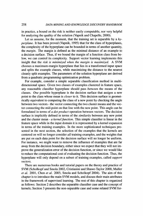
Chapter 12

SUPPORT VECTOR MACHINES

Armin Shmilovici Ben-Gurion Universiry

Abstract Support Vector Machines (SVMs) are a set of related methods for supervised learning, applicable to both classification and regression problems. A SVM classifiers creates a maximum-margin hyperplane that lies in a transformed input space and splits the example classes, while maximizing the distance to the nearest cleanly split examples. The parameters of the solution hyperplane are derived from a quadratic programming optimization problem. Here, we provide several formulations, and discuss some key concepts.

Keywords: Support Vector Machines, Margin Classifier, Hyperplane Classifiers, Support Vector Regression, Kernel Methods

1. Introduction Support Vector Machines (SVMs) are a set of related methods for super-

vised learning, applicable to both classification and regression problems. Since the introduction of the SVM classifier a decade ago (Vapnik, 1995), SVM gained popularity due to its solid theoretical foundation. The development of efficient implementations led to numerous applications (Isabelle, 2004).

The Support Vector learning machine was developed by Vapnik et al. (Scholkopf et al., 1995, Scholkopf 1997) to constructively implement princi- ples from statistical learning theory (Vapnik, 1998). In the statistical learning framework, learning means to estimate a function from a set of examples (the training sets). To do this, a learning machine must choose one function from a given set of functions, which minimizes a certain risk (the empirical risk) that the estimated function is different from the actual (yet unknown) function. The risk depends on the complexity of the set of functions chosen as well as on the training set. Thus, a learning machine must find the best set of functions - as determined by its complexity - and the best function in that set. Unfortunately,

25 8 DATA MINING AND KNOWLEDGE DISCOVERY HANDBOOK

in practice, a bound on the risk is neither easily computable, nor very helpful for analyzing the quality of the solution (Vapnik and Chapelle, 2000).

Let us assume, for the moment, that the training set is separable by a hyperplane. It has been proved (Vapnik, 1995) that for the class of hyperplanes, the complexity of the hyperplane can be bounded in terms of another quantity, the margin. The margin is defined as the minimal distance of an example to a decision surface. Thus, if we bound the margin of a function class from be- low, we can control its complexity. Support vector learning implements this insight that the risk is minimized when the margin is maximized, A SVM chooses a maximum-margin hyperplane that lies in a transformed input space and splits the example classes, while maximizing the distance to the nearest cleanly split examples. The parameters of the solution hyperplane are derived from a quadratic programming optimization problem.

For example, consider a simple separable classification method in multi- dimensional space. Given two classes of examples clustered in feature space, any reasonable classifier hyperplane should pass between the means of the classes. One possible hyperplane is the decision surface that assigns a new point to the class whose mean is closer to it. This decision surface is geomet- rically equivalent to computing the class of a new point by checking the angle between two vectors - the vector connecting the two cluster means and the vector connecting the mid-point on that line with the new point. This angle can be formulated in terms of a dot product operation between vectors. The decision surface is implicitly defined in terms of the similarity between any new point and the cluster mean - a kernelfunction. This simple classifier is linear in the feature space while in the input domain it is represented by a kernel expansion in terms of the training examples. In the more sophisticated techniques presented in the next section, the selection of the examples that the kernels are centered on will no longer consider all training examples, and the weights that are put on each data point for the decision surface will no longer be uniform. For instance, we might want to remove the influence of examples that are far away from the decision boundary, either since we expect that they will not improve the generalization error of the decision function, or since we would like to reduce the computational cost of evaluating the decision function. Thus, the hyperplane will only depend on a subset of training examples, called support vectors.

There are numerous books and tutorial papers on the theory and practice of SVM (Scholkopf and Smola 2002, Cristianini and Shawe-Taylor 2000, Muller et al. 2001, Chen et al. 2003, Smola and Scholkopf 2004). The aim of this chapter is to introduce the main SVM models, and discuss their main attributes in the framework of supervised learning. The rest of this chapter is organized as follows: Section 2 describes the separable classifier case and the concept of kernels; Section 3 presents the non-separable case and some related SVM for-

Support Vector Machines 259

mulations; Section 4 discusses some practical computational aspects; Section 5 discusses some related concepts and applications; and Section 6 concludes with a discussion.

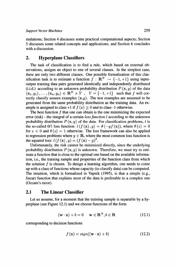
2. Hyperplane Classifiers The task of classification is to find a rule, which based on external ob-

servations, assigns an object to one of several classes. In the simplest case, there are only two different classes. One possible formalization of this classification task is to estimate a function f : RN + (-1, +1) using input- output training data pairs generated identically and independently distributed (i.i.d.) according to an unknown probability distribution P (x, y) of the data (xl, yl), . . . , (x,, y,) E RN x Y , Y = (-1, +1) such that f will cor- rectly classify unseen examples (x,y). The test examples are assumed to be generated from the same probability distribution as the training data. An example is assigned to class +1 if f (z) > 0 and to class -1 otherwise.

The best function f that one can obtain is the one minimizing the expected error (risk) - the integral of a certain lossfunction 1 according to the unknown probability distribution P (x, y) of the data. For classification problems, 1 is the so-called 011 loss function: 1 (f (x) , y) = 8 (-y f (x)), where 8 (z) = 0 for z < 0 and 8 (z) = 1 otherwise. The loss framework can also be applied to regression problems where y E R , where the most common loss function is

2 the squared loss: 1 (f (x) , y) = (f (x) - y) . Unfortunately, the risk cannot be minimized directly, since the underlying

probability distribution P (x, y) is unknown. Therefore, we must try to estimate a function that is close to the optimal one based on the available information, i.e., the training sample and properties of the function class from which the solution f is chosen. To design a learning algorithm, one needs to come up with a class of functions whose capacity (to classify data) can be computed. The intuition, which is formalized in Vapnik (1995), is that a simple (e.g., linear) function that explains most of the data is preferable to a complex one (Occam's razor).

2.1 The Linear Classifier Let us assume, for a moment that the training sample is separable by a hy-

perplane (see Figure 12.1) and we choose functions of the form

corresponding to decision functions

DATA MINING AND KNOWLEDGE DISCOVERY HANDBOOK

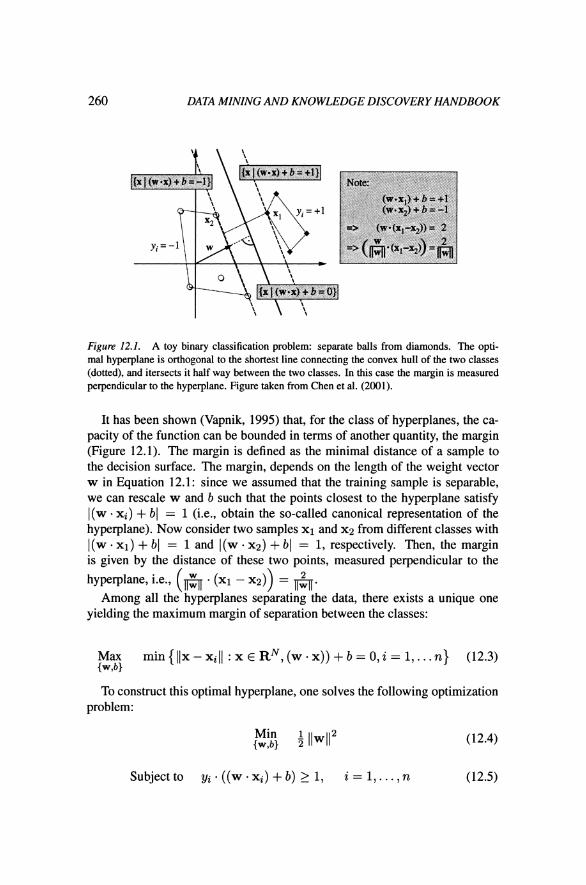
Figure 12.1. A toy binary classification problem: separate balls from diamonds. The optimal hyperplane is orthogonal to the shortest line connecting the convex hull of the two classes (dotted), and itersects it half way between the two classes. In this case the margin is measured perpendicular to the hyperplane. Figure taken from Chen et al. (2001).

It has been shown (Vapnik, 1995) that, for the class of hyperplanes, the capacity of the function can be bounded in terms of another quantity, the margin (Figure 12.1). The margin is defined as the minimal distance of a sample to the decision surface. The margin, depends on the length of the weight vector w in Equation 12.1: since we assumed that the training sample is separable, we can rescale w and b such that the points closest to the hyperplane satisfy I(w. xi) + bl = 1 (i.e., obtain the so-called canonical representation of the hyperplane). Now consider two samples xl and x2 from different classes with I(w . XI) + bl = 1 and I(w . x2) + bl = 1, respectively. Then, the margin is given by the distance of these two points, measured perpendicular to the

2 hyperplane, i.e., (a - (XI - x2)) = m. Among all the hyperplanes separating the data, there exists a unique one

yielding the maximum margin of separation between the classes:

Max m i n { ~ ~ ~ - ~ ~ ~ : x ~ ~ ~ , ( w - x ) ) + b = ~ , i = l , ... n ) (12.3) {wAJ)

To construct this optimal hyperplane, one solves the following optimization problem:

Subjectto yi - ((w .xi) + b) 1 1, i = 1, . . . , n (12.5)

Support Vector Machines 26 1

This constraint optimization problem can be solved by introducing Lagrange multipliers ai 1 0 and the Lagrangian function

The Langrangian L has to be minimized with respect to the primal variables {w, b ) and maximized with respect to the dual variables ai. The optimal point is a saddle point and we have the following equations for the primal variables:

which translate into

The solution vector thus has an expansion in terms of a subset of the training patterns. The Support Vectors are those patterns corresponding with the non- zero ai, and the non-zero ai are called Support Values. By the Karush-Kuhn- Tucker (KKT) complimentary conditions of optimization, the ai must be zero for all the constraints in Equation 12.5 which are not met as equality, thus

and all the Support Vectors lie on the margin (Figures 12.1,12.3) while the all remaining training examples are irrelevant to the solution. The hyperplane is completely captured by the patterns closest to it.

For a nonlinear problem like in the problem presented in Equations 12.4- 12.5, called a primal problem, under certain conditions, the primal and dual problems have the same objective values. Therefor, we can solve the dual problem which may be easier than the primal problem. In particular, when working in feature space (Section 2.3) solving the dual may be the only way to train the SVM. By substituting Equation 12.8 into Equation 12.6, one elim- inates the primal variables and arrives at the Wolfe dual (Wolfe, 1961) of the optimization problem for the multipliers ai:

n Subject to ai 2 0, i = 1 , . . . , n , aiyi = 0 (12.1 1)

i=l

262 DATA MINING AND KNOWLEDGE DISCOVERY HANDBOOK

The hyperplane decision function presented in Equation 12.2 can now be explicitly written as

where b is computed from Equation 12.9 and from the set of support vectors Xi,i E I = { i : a + #0).

2.2 The Kernel Trick The choice of linear classifier functions seems to be very limited (i.e., likely

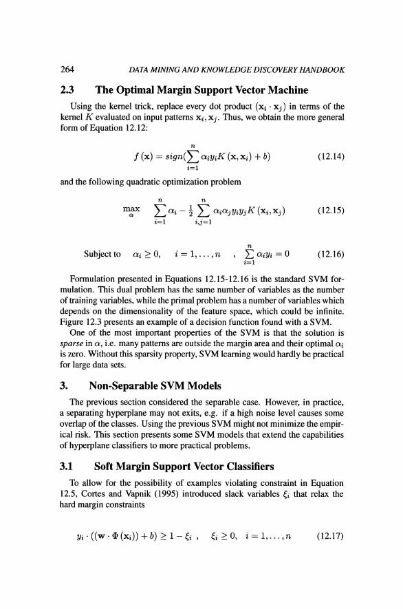
to underfit the data). Fortunately, it is possible to have both linear models and a very rich set of nonlinear decision functions by using the kernel trick (Cortes and Vapnik, 1995) with maximum-margin hyperplanes. Using the kernel trick for SVM makes the maximum margin hyperplane be fit in a feature space F. The feature space F is a non-linear map @ : R~ --+ F from the original input space, usually of much higher dimensionality than the original input space. With the kernel trick, the same linear algorithm is worked on the transformed data (@ ( x l ) , yl ) , . . . , (@ (x,) , yn). In this way, non-linear SVMs can makes the maximum margin hyperplane be fit in a feature space. Figure 12.2 demon- strates such a case. In the original (linear) training algorithm (see Equations 12.10-12.12) the data appears in the form of dot products xi - xj. Now, the training algorithm depends on the data through dot products in F, i.e., on functions of the form @ (x i ) @ ( x j ) . I f there exists a kernel function K such that K (x i , x j ) = @ (xi) @ ( x j ) , we would only need to use K in the training algorithm and would never need to explicitly even know what @ is.

Mercer's condition, (Vapnik, 1995) tells us the mathematical properties to check whether or not a prospective kernel is actually a dot product in some space, but it does not tell us how to construct @, or even what F is. Choosing the best kernel function is a subject of active research (Smola and Scholkopf 2002, Steinwart 2003). It was found that to a certain degree different choices of kernels give similar classification accuracy and similar sets of support vectors (Scholkopf et al. 1995), indicating that in some sense there exist "important" training points which characterize a given problem.

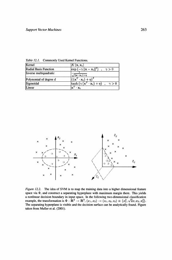
Some commonly used kernels are presented in Table 12.1. Note, however, that the Sigmoidal kernel only satisfies Mercer's condition for certain values of the parameters and the data. Hsu et al. (2003) advocate the use of the Radial Basis Function as a reasonable first choice.

Support Vector Machines

Table 12.1. Commonly Used Kernel Functions.

Figure 12.2. The idea of SVM is to map the training data into a higher dimensional feature space via a, and construct a separating hyperplane with maximum margin there. This yields a nonlinear decision boundary in input space. In the following two-dimensional classification example, the transformation is : R2 --, R3, (XI, 22) -+ (z1,z2, 23) EE (x:, 6 ~ 1 x 2 , ~ ; ) .

The separating hyperplane is visible and the decision surface can be analytically found. Figure taken from Muller et al. (2001).


2.3 The Optimal Margin Support Vector Machine Using the kernel trick, replace every dot product (xi - x j ) in terms of the

kernel K evaluated on input patterns xi, xj. Thus, we obtain the more general form of Equation 12.12:

and the following quadratic optimization problem

It

Subject to ai 2 0, i = 1, . . . , n , x aiyi = 0 (12.16) i=l

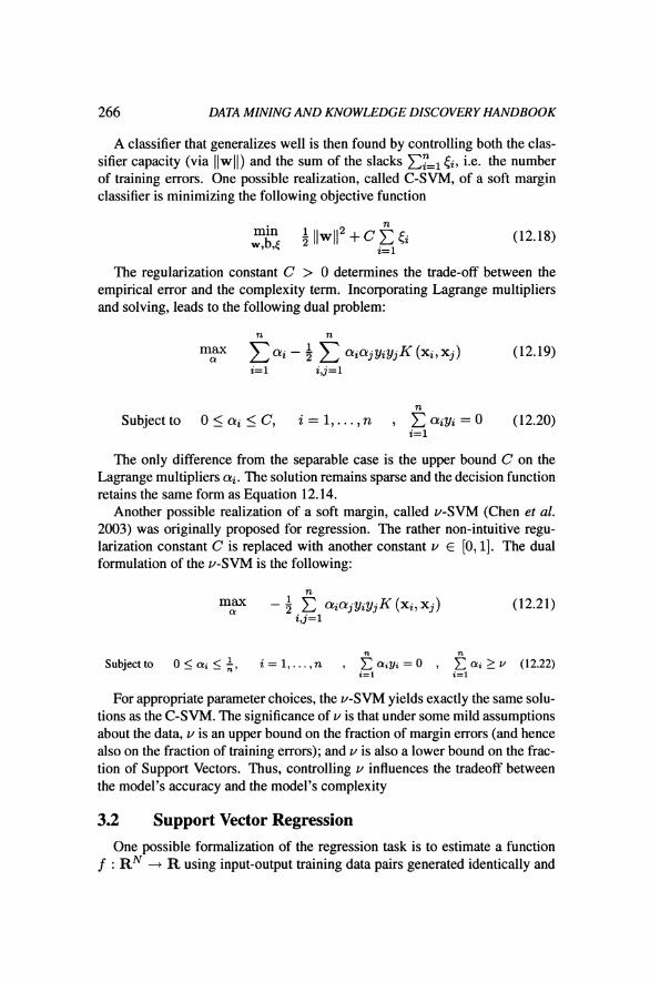
Formulation presented in Equations 12.15-12.16 is the standard SVM formulation. This dual problem has the same number of variables as the number of training variables, while the primal problem has a number of variables which depends on the dimensionality of the feature space, which could be infinite. Figure 12.3 presents an example of a decision function found with a SVM.

One of the most important properties of the SVM is that the solution is sparse in a, i.e. many patterns are outside the margin area and their optimal ai is zero. Without this sparsity property, SVM learning would hardly be practical for large data sets.

3. Non-Separable SVM Models The previous section considered the separable case. However, in practice,

a separating hyperplane may not exits, e.g. if a high noise level causes some overlap of the classes. Using the previous SVM might not minimize the empirical risk. This section presents some SVM models that extend the capabilities of hyperplane classifiers to more practical problems.

3.1 Soft Margin Support Vector Classifiers To allow for the possibility of examples violating constraint in Equation

12.5, Cortes and Vapnik (1995) introduced slack variables & that relax the hard margin constraints

Support Vector Machines

Figure 12.3. Example of a Support Vector classifier found by using a radial basis function kernel. Circles and disks are two classes of training examples. Ex- circles mark the S u p port Vectors found by the algorithm. The middle line is the decision surface. The outer lines precisely meet the constraint in Equation 12.16. The shades indicate the absolute value of the argument of the sign function in Equation 12.14. Figure taken from Chen et al. (2003).


A classifier that generalizes well is then found by controlling both the classifier capacity (via IIwII) and the sum of the slacks C:=, Q, i.e. the number of training errors. One possible realization, called C-SVM, of a soft margin classifier is minimizing the following objective function

min w , b ~ 4 llwl12 + c 5 t i

i=l

The regularization constant C > 0 determines the trade-off between the empirical error and the complexity term. Incorporating Lagrange multipliers and solving, leads to the following dual problem:

Subject to 0 < a i < C, i = 1,. . . , n , C a i y i = 0 (12.20) i=l

The only difference from the separable case is the upper bound C on the Lagrange multipliers a i . The solution remains sparse and the decision function retains the same form as Equation 12.14.

Another possible realization of a soft margin, called v-SVM (Chen et al. 2003) was originally proposed for regression. The rather non-intuitive regularization constant C is replaced with another constant v E [0, 11. The dual formulation of the v-SVM is the following:

max CY - 2 &ajy iy jK ( x i , x j )

i j = l

Subject to 0 5 a i 5 i, i = 1,. . . ,n , i=l 5 a i y i = 0 ,

For appropriate parameter choices, the v-SVM yields exactly the same solutions as the C-SVM. The significance of v is that under some mild assumptions about the data, v is an upper bound on the fraction of margin errors (and hence also on the fraction of training errors); and v is also a lower bound on the fraction of Support Vectors. Thus, controlling v influences the tradeoff between the model's accuracy and the model's complexity

3.2 Support Vector Regression One possible formalization of the regression task is to estimate a function

f : R~ -+ R using input-output training data pairs generated identically and


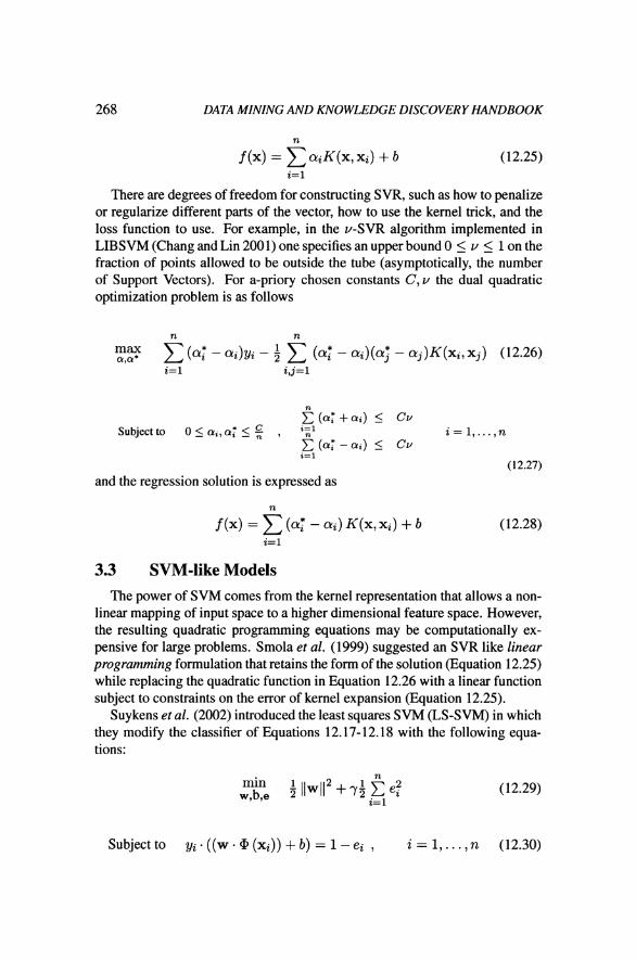
independently distributed (i.i.d.) according to an unknown probability distribution P (x, y ) of the data. The concept of margin is specific to classification. However, we would still like to avoid too complex regression functions. The idea of SVR (Smola and Scholkopf, 2004) is that we find a function that has at most E deviation from the actually obtained targets yi for all the training data, and at the same time is as flat as possible. In other words, errors are unirnpor- tant as long as they are less then E, but we do not tolerate deviations larger than this. An analogue of the margin is constructed in the space of the target values y E R. By using Vapnik's €-sensitive loss function (Figure 12.4).

A tube with radius E is fitted to the data, and a regression function that generalizes well is then found by controlling both the regression capacity (via 11~11) and the loss function. One possible realization, called C-SVR, of a is minimizing the following objective function

The regularization constant C > 0 determines the trade-off between the empirical error and the complexity term.

Figure 12.4. In SV regression, a tube with radius E is fitted to the data. The optimization determines a trade-off between model complexity and points lying outside of the tube. Figure taken From Smola and Scholkopf (2004).

Generalization to kernel-based regression estimation is carried out in com- plete analogy with the classification problem. Introducing Lagrange multipliers and choosing a-priory the regularization constants C, E one arrives at a dual quadratic optimization problem. The support vectors and the support values of the solution define the following regression function

DATA MINING AND KNOWLEDGE DISCOVERY HANDBOOK

n

f ( x ) = C a i K ( x , x i ) + b (12.25) i=l

There are degrees of freedom for constructing SVR, such as how to penalize or regularize different parts of the vector, how to use the kernel trick, and the loss function to use. For example, in the v-SVR algorithm implemented in LIBSVM (Chang and Lin 2001) one specifies an upper bound 0 I v 5 1 on the fraction of points allowed to be outside the tube (asymptotically, the number of Support Vectors). For a-priory chosen constants C, v the dual quadratic optimization problem is as follows

2 (at +a;) 5 cv %=I Subject to 0 5 ai, at 5 , C (at - a;) 5 CV i=l

and the regression solution is expressed as

n

f ( x ) = C (a; - ai) K ( x , xi) + b i=l

3.3 SVM-like Models The power of SVM comes from the kernel representation that allows a non-

linear mapping of input space to a higher dimensional feature space. However, the resulting quadratic programming equations may be computationally ex- pensive for large problems. Smola et al. (1999) suggested an SVR like linear programming formulation that retains the form of the solution (Equation 12.25) while replacing the quadratic function in Equation 12.26 with a linear function subject to constraints on the error of kernel expansion (Equation 12.25).

Suykens et al. (2002) introduced the least squares SVM (LS-SVM) in which they modify the classifier of Equations 12.17-12.18 with the following equations:

min wb,e

Subject to yi li ((w - ( x i ) ) + b) = 1 - ei , i = 1,. . . , n (12.30)


Important differences with standard SVM are the equality constraint (see Equation 12.30) and the sum squared error terms, which greatly simplify the problem. Incorporating Lagrange multipliers and solving leads to the following dual linear problem:

where the primal variables {w, b) define as before a decision surface like Equa- tion 12.14, Y = (yl, . . . , y,), (a)$ . = yiyjK (xi, xj), I, 0 are appropriate

d size all ones (all zeros) matrices, and y is a tuning parameter to be optimized. Equivalently, modifying the regression problem presented in Equations 12.26- 12.27 also results in a linear system like (Equation 12.31) with an additional tuning parameter.

The LS-SVM can realize strongly nonlinear decision boundaries, and efficient matrix inversion methods can handle very large datasets. However, a is not sparse anymore (Suykens et al. 2002).

4. Implementation Issues with SVM The purpose of this section is to overview some problems that face the ap-

plication of SVM in machine learning.

4.1 Optimization Techniques The solution of the SVM problem, is the solution of a constraint (convex)

quadratic programming (QP) problem such as Equations 12.15-12.16. Equa- tion 12.15 can be rewritten as maximizing -;aTKa + lTa, where l is a vector of all ones and k j = yiyjk (xi, xj). When the Hessian matrix K is positive definite, the objective function is convex and there is a unique global solution. If matrix K is positive semi-definite, every maximum is also a global maximum, however, there can be several optimal solutions (different in their a) which might lead to different performance on the testing dataset.

In general, the support vector optimization can be solved analytically only when the number of training data is very small. The worst case computational complexity for the general analytic case results from the inversion of the Hessian matrix, thus is of order N:, where Ns is the number of support vectors. There exists a vast literature on solving quadratic programs (Bert- sekas 1995, Bazaraa et al. 1993) and several software packages are available. However, most quadratic programming algorithms are either only suitable for small problems or assume that the Hessian matrix K is sparse, i.e., most elements of this matrix are zero. Unfortunately, this is not true for the SVM problem. Thus, using standard quadratic programming codes with more than a few hundred variables results in enormous training times and more demanding


memory needs. Nevertheless, the structure of the SVM optimization problem allows the derivation of specially tailored algorithms, which allow for fast convergence with small memory requirements, even on large problems.

A key observation in solving large-scale SVM problems is the sparsity of the solution (Steinwart, 2004). Depending on the problem, many of the optimal Qi will either be zero or on the upper bound. If one could know beforehand which ai were zero, the corresponding rows and columns could be removed from the matrix K without changing the value of the quadratic form. Furthermore, a point can only be optimal if it fulfills the KKT conditions (such as Equation 12.5). SVM solvers decompose the quadratic optimization problem into a sequence of smaller quadratic optimization problems that are solved in sequence. Decomposition methods are based on the observations of Osuna et al. (1997) that each QP in a sequence of QPs always contains at least one sample violating the KKT conditions. The classifier built from solving the QP for part of the training data is used to test the rest of the training data. The next partial training set is generated from combining the support vectors already found (the "working set") with the points that most violate the KKT conditions, such that the partial Hessian matrix will fit the memory. The algorithm will eventually converge to the optimal solution. Decomposition methods differ in the strategies for generating the smaller problems and use sophisticated heuristics to select several patterns to add and remove from the sub-problem plus efficient caching methods. They usually achieve fast convergence even on large data sets with up to several thousands of support vectors. A quadratic optimizer is still required as part of the solver. Elements of the SVM solver can take ad- vantage of parallel processing: such as simultaneous computing of the Hessian matrix, dot products, and the objective function. More details and tricks can be found in the literature (Platt, 1998, Joachims 1999, Smola et al. 2000, Lin 2001, Chang and Lin 2001, Chew et al. 2003, Chung et al. 2004).

A fairly large selection of optimization codes for SVM classification and regression may be found on the Web (Kernel 2004), together with the appropriate references. They range from simple MATLAB implementation to sophisticated C, C++, or FORTRAN programs (e-g., LIBSVM: Chang and Lin 2001, SVMlight: Joachim 2004). Some solvers include integrated model selection and data rescaling procedures for improved speed and numerical stability. Hsu et al. (2003) advises about working with a SVM software on practical problems.

4.2 Model Selection To obtain a high level of performance, some parameters of the SVM algo-

rithm have to be tuned. These include 1) the selection of the kernel function; 2) the kernel parameter(s); 3) the regularization parameters (C, v, E ) for the

Support Vector Machines 27 1

tradeoff between the model complexity and the model accuracy. Model selection techniques provide principled ways to select a proper kernel. Usually, a sequence of models is solved, and using some heuristic rules, next set of parameters is tested. The process is continued until a given criterion is obtained (e.g., 99% correct classification). For example, if we consider 3 alternative (single parameter) kernels, 5 partitions of the kernel parameters, and one regularization parameters with 5 partitions each, then we need to consider a total of 3x5x5=125 SVM evaluations.

The cross validation technique is widely used for a prediction of the generalization error, and is included in some SVM packages (such as LIBSVM: Chang and Lin 2001). Here, the training samples are divided into k subsets of equal size. Then, the classifier is trained k times: in the i-th iteration (i = 1, ..., k), the classifier is trained on all subsets except the i-th one. Then, the classification error is computed for the i-th subset. It is known that the average of these k errors is a rather good estimate of the generalization error. k is typ- ically 5 or 10. Thus, for the example above we need to consider at least 625 SVM evaluations to identify the model of the best SVM classifier.

In the Bayesian evidence framework the training of an SVM is interpreted as Bayesian inference, and the model selection is accomplished by maximizing the marginal likelihood (i.e., evidence). Law and Kwok (2000) and Chu (2003) provide iterative parameter updating formulas, and report a significantly smaller number of SVM evaluations.

4.3 Multi-Class SVM Though SVM was originally designed for two-class problems, several ap-

proaches have been developed to extend SVM for multi-class data sets. One approach to k-class pattern recognition is to consider the problem as

a collection of binary classification problems. The technique of one-against- the-rest requires k binary classifiers to be constructed (when the label +1 is assigned to each class in its turn and the label -1 is assigned to the other k - 1 classes). In the prediction stage, a voting scheme is applied to classify a new point. In the winner-takes-all voting scheme, one assigns the class with the largest real value. The one-against-one approach trains a binary SVM for any two classes of data and obtains a decision function. Thus, for a k-class problem, there are k(k - 1)/2 decision functions where the voting scheme is desig- nated to choose the class with the maximum number of votes. More elaborate voting schemes, such as error-correcting-codes consider the combined outputs from the n-parallel classifiers as a binary n-bit code word and selects the class with the closest (e.g. Hamming distance) code.

In Hsu and Lin (2002), it was experimentally shown that for general problems, using the C-SVM classifier, various multi-class approaches give similar


accuracy. Rifkin and Klautau (2004) have similar observation, however, this may not always be the case. Multi-class methods must be considered together with parameter-selection strategies. That is, we search for appropriate regularization parameters and kernel parameters for constructing a better model. Chen, Lin and Scholkopf (2003) experimentally demonstrate inconsistent and marginal improvement in the accuracy when the parameters are trained differ- ently for each classifier inside a multi-class C-SVM and V-SVM classifiers.

5. Extensions and Application Kernel algorithms have solid foundations in statistical learning theory and

functional analysis, thus, kernel methods combine statistics and geometry. Ker- nels provide an elegant framework for studying fundamental issues of machine learning, such as similarity measures that can incorporate prior knowledge about the problem, and data representations. SVM have been one of the major kernel methods for supervised learning. It is not surprising that recent methods integrate SVM with kernel methods (Scholkopf et al. 1999, Scholkopf and Smola, 2002, Shawe-Taylor and Cristianini 2004) for unsupervised learning problems such as density estimation (Weston and Herbrich, 2000).

SVM has a strong analogy in regularization theory (Williamson et al., 2001). Regularization is a method of solving problems by making some a- priori assumptions about the desired function. A penalty term that discourages over-fitting is added to the error function. A common choice of regularizer is given by the sum of the squares of the weight parameters and results in a functional similar to Equation 12.6. Like SVM, optimizing a functional of the learning function, such as its smoothness, leads to sparse solutions.

Boosting is a machine learning technique that attempts to improve a "weak" learning algorithm, by a convex combination of the original "weak" learning function, each one trained with a different distribution of the data in the training set. SVM can be translated to a corresponding boosting algorithm using the appropriate regularization norm (Ratsch et al., 2001).

Successful applications of SVM algorithms have been reported for various fields, such as pattern recognition (Martin et al. 2002), text categorization (Dumais 1998, Joachims 2002), time series prediction (Mukherjee, 1997), and bio-informatics (Zien et al. 2000). Historically, classification experiments with the U.S. Postal Service benchmark problem - the first real-world experiment of SVM (Cortes and Vapnik 1995, Scholkopf 1995) - demonstrated that plain SVMs give a performance very similar to other state-of-the-art methods. SVM has been achieving excellent results also on the Reuters-22173 text classification benchmark problem (Dumais, 1998). SVMs have been strongly improved by using prior knowledge about the problem to engineer the kernels and the support vectors with techniques such as virtual support vectors (Scholkopf


1997, Scholkopf et al. 1998). Isabelle (2004) and Kernel (2004) present many more applications.

6. Conclusion Since the introduction of the SVM classifier a decade ago, SVM gained

popularity due to its solid theoretical foundation in statistical learning theory. They differ radically from comparable approaches such as neural networks: they have a simple geometrical interpretation and SVM training always finds a global minimum. The development of efficient implementations led to numerous applications. Selected real-world applications served to exemplify that SVM learning algorithms are indeed highly competitive on a variety of problems.

SVM are a set of related methods for supervised learning, applicable to both classification and regression problems. This chapter provides an overview of the main SVM methods for the separable and non-separable case and for classification and regression problems. However, SVM methods are being extended to unsupervised learning problems.

A SVM is largely characterized by the choice of its kernel. The kernel can be viewed as a nonlinear similarity measure, and should ideally incorporate prior knowledge about the problem at hand. The best choice of kernel for a given problem is still an open research issue. A second limitation is the speed of training. Training for very large datasets (millions of support vectors) is still an unsolved problem.

References Bazaraa M. S., Sherali H. D., and Shetty C. M. Nonlinear programming: theory

and algorithms. Wiley, second edition, 1993. Bertsekas D.P. Nonlinear Programming. Athena Scientific, MA, 1995. Chang C.-C. and Lin C.-J. Training support vector classifiers: Theory and al-

gorithms. Neural Computation 2001 ; 13(9):2119-2147. Chang C.-C. and Lin C.-J. (2001). LIBSVM: a library for support vector ma-

chines. Software available at http://www.csie.ntu.edu.tw/~cjlin/libsvm. Chen P.-H., Lin C. -J., and Scholkopf B. A tutorial on nu-support vector ma-

chines. 2003. Chew H. G., Lim C. C., and Bogner R. E. An implementation of training dual-

nu support vector machines. In Qi, Teo, and Yang, editors, Optimization and Control with Applications. Kluwer, 2003.

Chu W. Bayesian approach to support vector machines. PhD thesis, National University of Singapore , 2003; Available online http://citeseer.ist.psu.edu/ chu03bayesian.html


Chung K.-M., Kao W.-C., Sun C.-L., and Lin C.-J. Decomposition methods for linear support vector machines. Neural Computation 2004; 16(8):1689- 1704).

Cortes C. and Vapnik V. Support vector networks. Machine Learning 1995; 20~273-297.

Cristianini N. and Shawe-Taylor J. An Introduction to Support Vector Ma- chines and other kernel-based learning methods. Cambridge Univ. Press, 2000.

Dumais S. Using SVMs for text categorization. IEEE Intelligent Systems 1998; 13(4).

Hsu C.-W. and Lin C.-J. A comparison of methods for multi-class support vector machines IEEE Transactions on Neural Networks 2002; 13(2); 415- 425.

Hsu C.-W. Chang C.-C and Lin C.-J. A practical guide to support vector classification. 2003. Available Online: www.csie.ntu.edu.tw/~cjlin/papers/guide /guide.pdf

Isabelle 2004, (a collection of SVM applications) Available Online: http:/l www.clopinet.com/isabelleProjects/SVWM/applist.html

Joachims T. Making large-scale SVM learning practical. In Scholkopf B., Burges C. J. C., and Smola A. J., editors, Advances in Kernel Methods - Support Vector Learning, pages 169-184, Cambridge, MA, MIT Press, 1999.

Joachims T. Learning to Classify Text using Support Vector Machines Meth- ods, Theory, and Algorithms. Kluwer Academic Publishers, 2002.

Joachims T. 2004, SVMlight, available online http://www.cs.cornell.edu /People/tj/svmlight/

Kernel 2004, (a collection of literature, software and Web pointers dealing with SVM and Gaussian processes) Available Online http://www.kernel- machines.org.

Law M. H. and Kwok J. T. Bayesian support vector regression. Proceedings of the 8th International Workshop on Artificial Intelligence and Statistics (AISTATS) pages 239-244, Key-West, Florida, USA, January 2000.

Lin C.-J. Formulations of support vector machines: a note from an optimization point of view. Neural Computation 2001 ; l3(2):307-3 17.

Lin C.-J. On the convergence of the decomposition method for support vector machines. IEEE Transactions on Neural Networks 2001; 12(6): 1288-1298.

Martin D. R., Fowlkes C. C., and Malik J. Learning to detect natural image boundaries using brightness and texture. In Advances in Neural Information Processing Systems, volume 14,2002.

Mukherjee S., Osuna E., and Girosi F. Nonlinear prediction of chaotic time series using a support vector machine. In Principe J., Gile L., Morgan N. and


Wilson E. editors, Neural Networks for Signal Processing VII - proceedings of the 1997 IEEE Workshop, pages 51 1-520, New-York, IEEE Press, 1997.

Muller K.-R., Mika S., Ratsch G., Tsuda K., and Scholkopf B., An introduction to kernel-based learning algorithms. IEEE Neural Networks 2001; 12(2):181-201.

Osuna E., Freund R., and Girosi F. An improved training algorithm for support vector machines. In Principe J., Gile L., Morgan N. and Wilson E. editors, Neural Networks for Signal Processing VII - proceedings of the 1997 IEEE Workshop, pages 276-285, New-York, IEEE Press, 1997.

Platt J. C. Fast training of support vector machines using sequential minimal optimization. In Scholkopf B., Burges C. J. C., and Smola A. J., editors, Advances in Kernel Methods - Support Vector Learning, Cambridge, MA, MIT Press, 1998.

Ratsch G., Onoda T., and Muller K.R. Soft margins for AdaBoost. Machine Learning 2001; 42(3):287-320.

Rifkin R. and Klautau A.. In Defense of One-vs-All Classification, Journal of Machine Learning Research 2004; 5: 101-141.

Scholkopf B., Support Vector Learning. Oldenbourg Verlag, Munich, 1997. Scholkopf B., Statistical learning and kernel methods, Technical Report MSR-

TR-2000-23, Available Online http://research.microsoft.com/research/pubs /view.aspx?msr-kid= MSR-TR-2000-23

Scholkopf B., Burges C.J.C., and Vapnik V.N. Extracting support data for a given task. In Fayyad U.M. and Uthurusamy R., Editors, Proceedings, First International Conference on Knowledge Discovery and Data Mining. AAAI Press, Menlo Park, CA, 1995.

Scholkopf B., Simard P.Y., Smola A.J., and Vapnik V.N.. Prior knowledge in support vector kernels. In Jordan M., Kearns M., and Solla S., Editors, Ad- vances in Neural Information Processing Systems 10, pages 640446. MIT Press, Cambridge, MA, 1998.

Scholkopf B., Burges C. J. C., and Smola A. J., editors, Advances in Kernel Methods - Support Vector Learning, Cambridge, MA, MIT Press, 1999.

Scholkopf B. and Smola A. J. Learning with Kernels. MIT Press, Cambridge, MA, 2002.

Scholkopf B., Smola A. J., Williamson R. C., and Bartlett P. L. New support vector algorithms. Neural Computation 2000; 12: 1207-1 245.

Shawe-Taylor J. and Cristianini N. Kernel Methods for Pattern Analysis. Cam- bridge University Press, 2004.

Smola A. J., Bartlett P. L., Scholkopf B. and Schuurmans D. Advances in Large Margin Classifiers. MIT Press, Cambridge, MA, 2000.

Smola A.J. and Scholkopf B.. A tutorial on support vector regression. Statistics and Computing 2004; 14(13):199-222.


Smola A.J., Scholkopf B. and Ratsch G. Linear programs for automatic accuracy control in regression. Proceedings of International Conference on Artificial Neural Networks ICANN'99, Berlin, Springer 1999.

Steinwart I. On the optimal parameter choice for nu-support vector machines. IEEE Transactions on Pattern Analysis and Machine Intelligence 2003; 25: 1274-1284.

Steinwart I. Sparseness of support vector machines. Journal of Machine Learn- ing Research 2004; 4(6): 107 1- 1 105.

Suykens J.A.K., Van Gestel T., De Brabanter J., De Moor B., and Vandewalle J. Least Squares Support Vector Machines. World Scientific Publishing, Sin- gapore, 2002.

Vapnik V. The Nature of Statistical Learning Theory . Springer Verlag, New York, 1995.

Vapnik V. Statistical Learning Theory. Wiley, NY, 1998. Vapnik V. and Chapelle 0. Bounds on error expectation for support vector

machines. Neural Computation 2000; 12(9):2013-2036. Weston J. and Herbrich R., Adaptive margin support vector machines. In Smola

A.J., Bartlett P.L., Scholkopf B., and Schuurmans D., Editors, Advances in Large Margin Classifiers, pages 281-296, MIT Press, Cambridge, MA, 2000,.

Williamson R. C., Smola A. J., and Scholkopf B., Generalization performance of regularization networks and support vector machines via entropy num- bers of compact operators. IEEE Transactions on Information Theory 2001; 47(6):25 16-2532.

Wolfe P. A duality theorem for non-linear programming. Quartely of Applied Mathematics 196 1; 19:239-244.

Zien A., Ratsch G., Mika S., Scholkopf B., Lengauer T. and Muller K.R. Engi- neering support vector machine kernels that recognize translation initiation sites. Bio-Informatics 2000; 16(9):799-807.

Documents

Data Mining and Knowledge Discovery Handbook || Support Vector Machines