Embed Size (px)
Citation preview
Data MiningAssociation Rules: Advanced Concepts
and Algorithms
Lecture Notes for Chapter 7
Introduction to Data Miningby
Tan, Steinbach, Kumar
(modified by Predrag Radivojac, 2018)
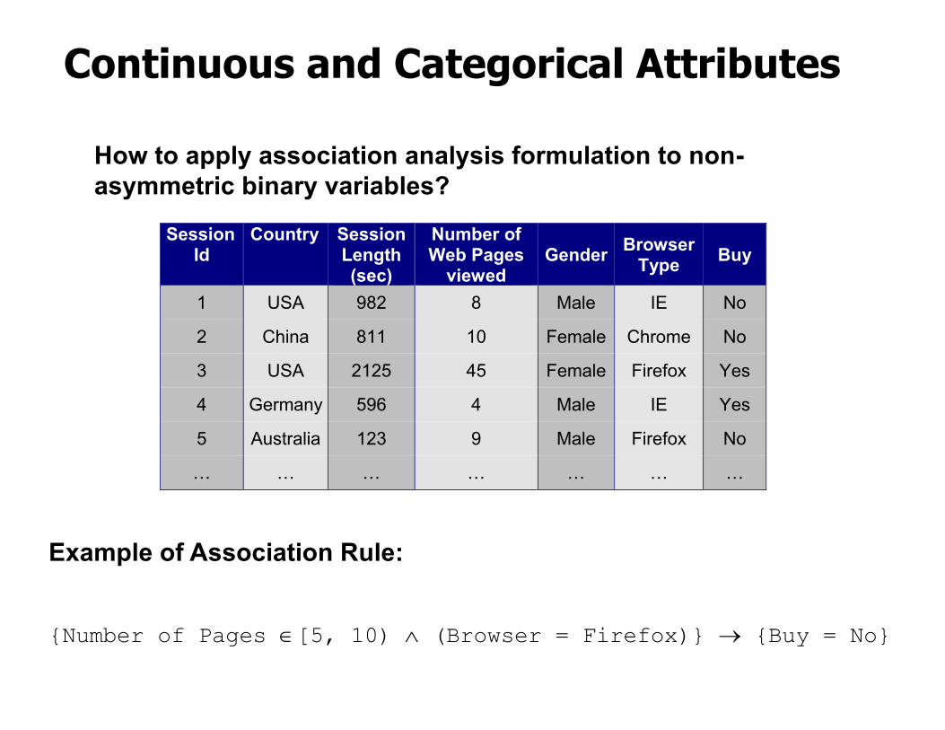
Continuous and Categorical Attributes
Session Id
Country Session Length (sec)
Number of Web Pages
viewed Gender Browser
Type Buy
1 USA 982 8 Male IE No
2 China 811 10 Female Chrome No
3 USA 2125 45 Female Firefox Yes
4 Germany 596 4 Male IE Yes
5 Australia 123 9 Male Firefox No
… … … … … … … 10
Example of Association Rule:
{Number of Pages Î[5, 10) Ù (Browser = Firefox)} ® {Buy = No}
How to apply association analysis formulation to non-asymmetric binary variables?
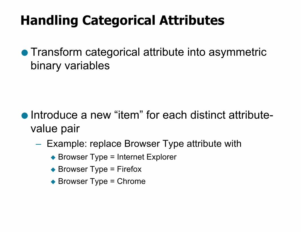
Handling Categorical Attributes
● Transform categorical attribute into asymmetric binary variables
● Introduce a new “item” for each distinct attribute-value pair– Example: replace Browser Type attribute with
u Browser Type = Internet Exploreru Browser Type = Firefoxu Browser Type = Chrome
Handling Categorical Attributes
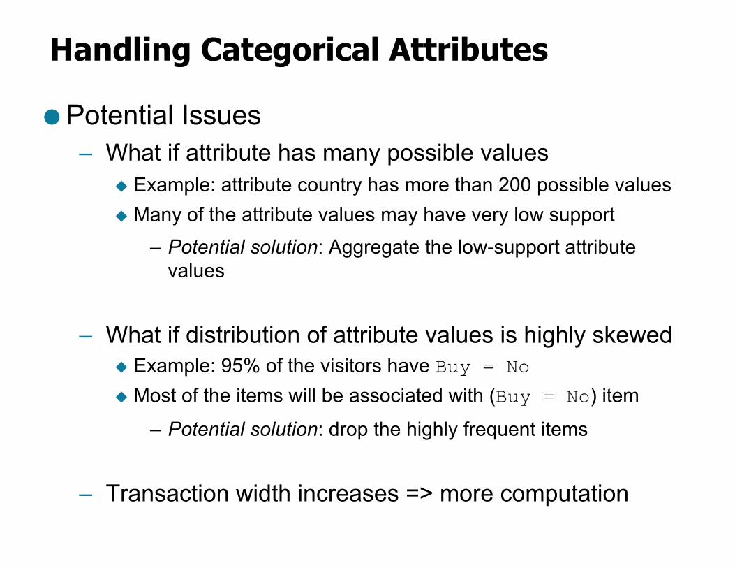
● Potential Issues– What if attribute has many possible values
u Example: attribute country has more than 200 possible valuesu Many of the attribute values may have very low support
– Potential solution: Aggregate the low-support attribute values
– What if distribution of attribute values is highly skewedu Example: 95% of the visitors have Buy = Nou Most of the items will be associated with (Buy = No) item
– Potential solution: drop the highly frequent items
– Transaction width increases => more computation
Handling Continuous Attributes
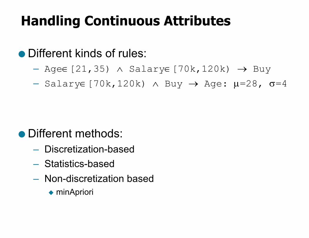
● Different kinds of rules:– AgeÎ[21,35) Ù SalaryÎ[70k,120k) ® Buy– SalaryÎ[70k,120k) Ù Buy ® Age: µ=28, s=4
● Different methods:– Discretization-based– Statistics-based– Non-discretization based
u minApriori
Handling Continuous Attributes
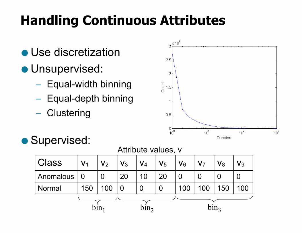
● Use discretization● Unsupervised:
– Equal-width binning– Equal-depth binning– Clustering
● Supervised:
Class v1 v2 v3 v4 v5 v6 v7 v8 v9
Anomalous 0 0 20 10 20 0 0 0 0Normal 150 100 0 0 0 100 100 150 100
bin1 bin3bin2
Attribute values, v
Discretization Issues
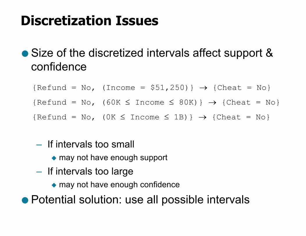
● Size of the discretized intervals affect support & confidence
– If intervals too smallu may not have enough support
– If intervals too largeu may not have enough confidence
● Potential solution: use all possible intervals
{Refund = No, (Income = $51,250)} ® {Cheat = No}
{Refund = No, (60K £ Income £ 80K)} ® {Cheat = No}
{Refund = No, (0K £ Income £ 1B)} ® {Cheat = No}
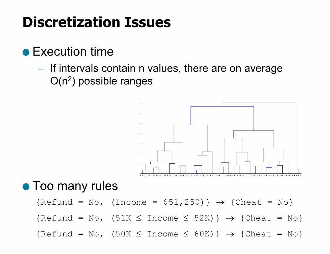
Discretization Issues
● Execution time– If intervals contain n values, there are on average
O(n2) possible ranges
● Too many rules{Refund = No, (Income = $51,250)} ® {Cheat = No}
{Refund = No, (51K £ Income £ 52K)} ® {Cheat = No}
{Refund = No, (50K £ Income £ 60K)} ® {Cheat = No}
Approach by Srikant & Agrawal
● Preprocess the data– Discretize attribute using equi-depth partitioning
u Use partial completeness measure to determine number of partitionsu Merge adjacent intervals as long as support is less than max-support
● Apply existing association rule mining algorithms
● Determine interesting rules in the output
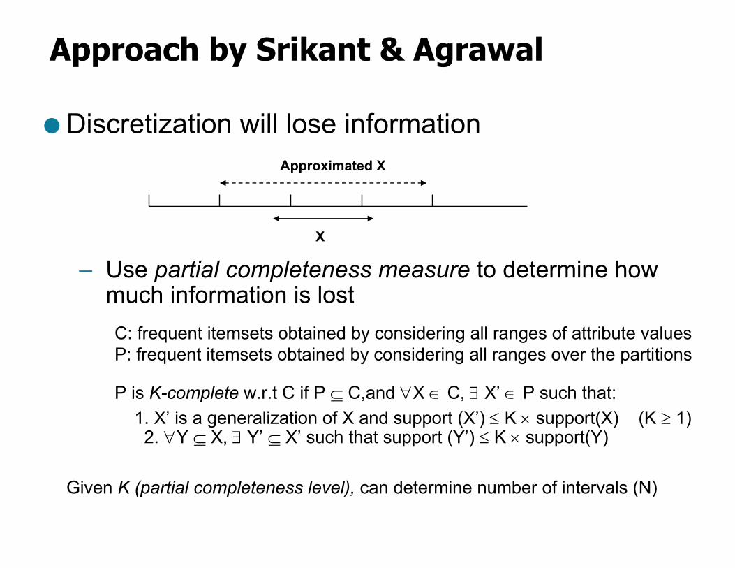
Approach by Srikant & Agrawal
● Discretization will lose information
– Use partial completeness measure to determine how much information is lost C: frequent itemsets obtained by considering all ranges of attribute valuesP: frequent itemsets obtained by considering all ranges over the partitions
P is K-complete w.r.t C if P Í C,and "X Î C, $ X’ Î P such that:1. X’ is a generalization of X and support (X’) £ K ´ support(X) (K ³ 1)2. "Y Í X, $ Y’ Í X’ such that support (Y’) £ K ´ support(Y)
Given K (partial completeness level), can determine number of intervals (N)
X
Approximated X
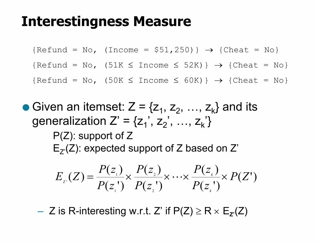
Interestingness Measure
● Given an itemset: Z = {z1, z2, …, zk} and its
generalization Z’ = {z1’, z2’, …, zk’}
P(Z): support of Z
EZ’(Z): expected support of Z based on Z’
– Z is R-interesting w.r.t. Z’ if P(Z) ³ R ´ EZ’(Z)
{Refund = No, (Income = $51,250)} ® {Cheat = No}
{Refund = No, (51K £ Income £ 52K)} ® {Cheat = No}
{Refund = No, (50K £ Income £ 60K)} ® {Cheat = No}
)'()'()(
)'()(
)'()()(
2
2
1
1
'ZP
zPzP
zPzP
zPzPZE
k
k
Z´´´´= !
Interestingness Measure
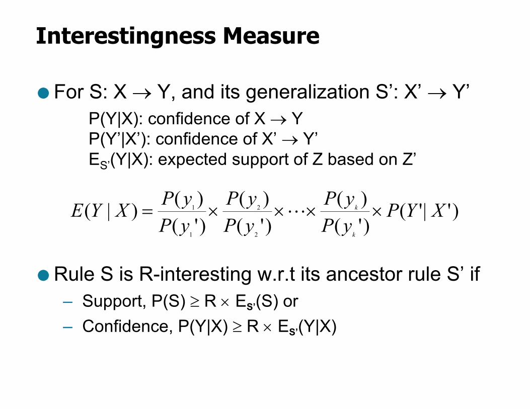
● For S: X ® Y, and its generalization S’: X’ ® Y’P(Y|X): confidence of X ® YP(Y’|X’): confidence of X’ ® Y’ES’(Y|X): expected support of Z based on Z’
● Rule S is R-interesting w.r.t its ancestor rule S’ if – Support, P(S) ³ R ´ ES’(S) or – Confidence, P(Y|X) ³ R ´ ES’(Y|X)
)'|'()'()(
)'()(
)'()()|(
2
2
1
1 XYPyPyP
yPyP
yPyPXYE
k
k ´´´´= !
Statistics-based Methods
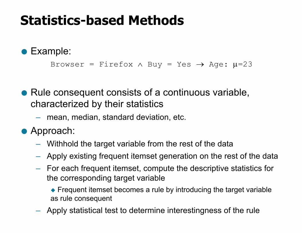
● Example: Browser = Firefox Ù Buy = Yes ® Age: µ=23
● Rule consequent consists of a continuous variable, characterized by their statistics
– mean, median, standard deviation, etc.
● Approach:– Withhold the target variable from the rest of the data– Apply existing frequent itemset generation on the rest of the data– For each frequent itemset, compute the descriptive statistics for
the corresponding target variableu Frequent itemset becomes a rule by introducing the target variable as rule consequent
– Apply statistical test to determine interestingness of the rule
Statistics-based Methods
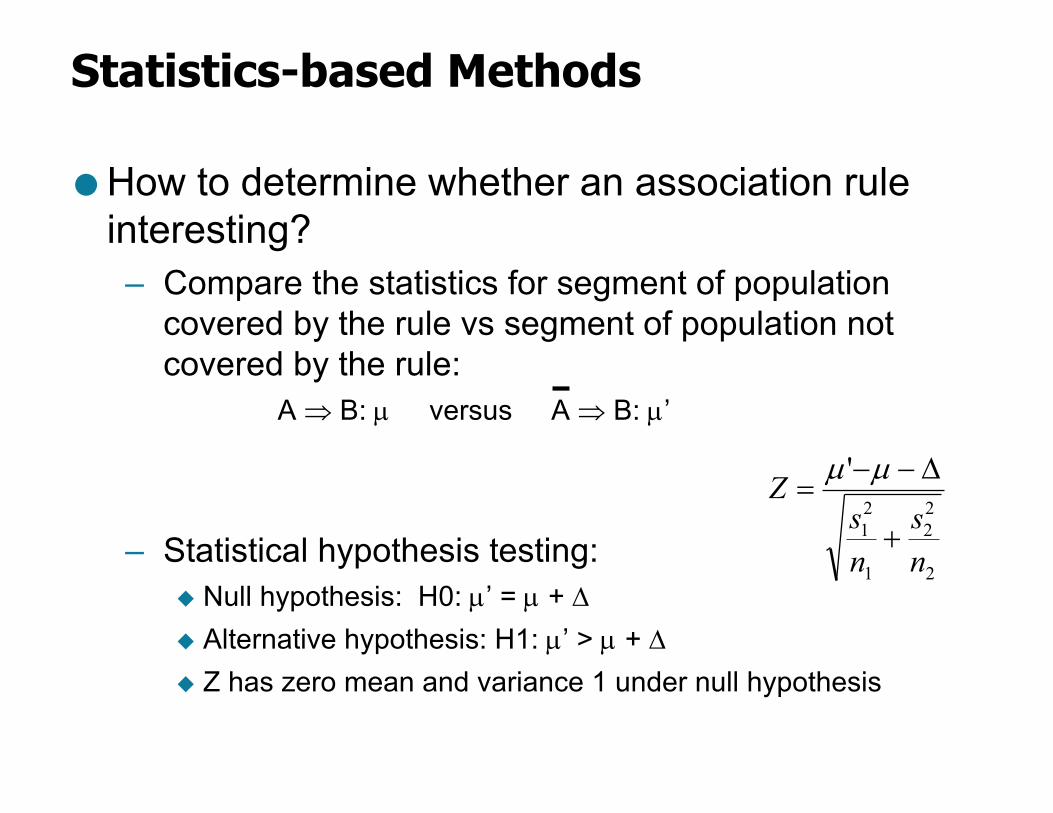
● How to determine whether an association rule interesting?– Compare the statistics for segment of population
covered by the rule vs segment of population not covered by the rule:
A Þ B: µ versus A Þ B: µ’
– Statistical hypothesis testing:u Null hypothesis: H0: µ’ = µ + Du Alternative hypothesis: H1: µ’ > µ + Du Z has zero mean and variance 1 under null hypothesis
2
22
1
21
'
ns
ns
Z+
D--=
µµ
Statistics-based Methods
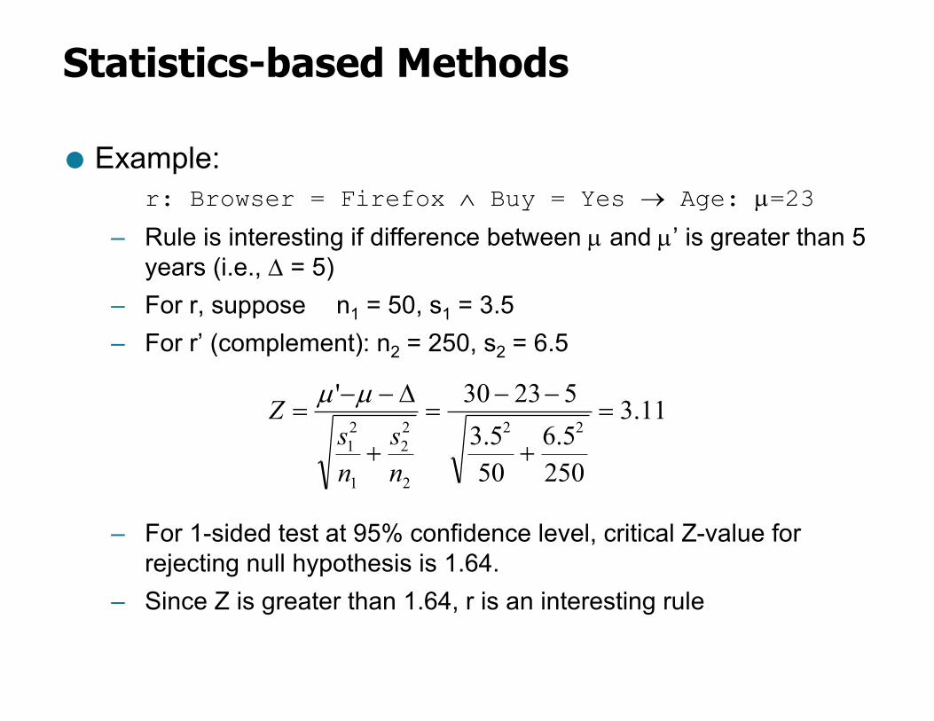
● Example: r: Browser = Firefox Ù Buy = Yes ® Age: µ=23
– Rule is interesting if difference between µ and µ’ is greater than 5 years (i.e., D = 5)
– For r, suppose n1 = 50, s1 = 3.5
– For r’ (complement): n2 = 250, s2 = 6.5
– For 1-sided test at 95% confidence level, critical Z-value for rejecting null hypothesis is 1.64.
– Since Z is greater than 1.64, r is an interesting rule
11.3
2505.6
505.3
52330'22
2
22
1
21
=
+
--=
+
D--=
ns
ns
Z µµ
Min-Apriori (Han et al.)
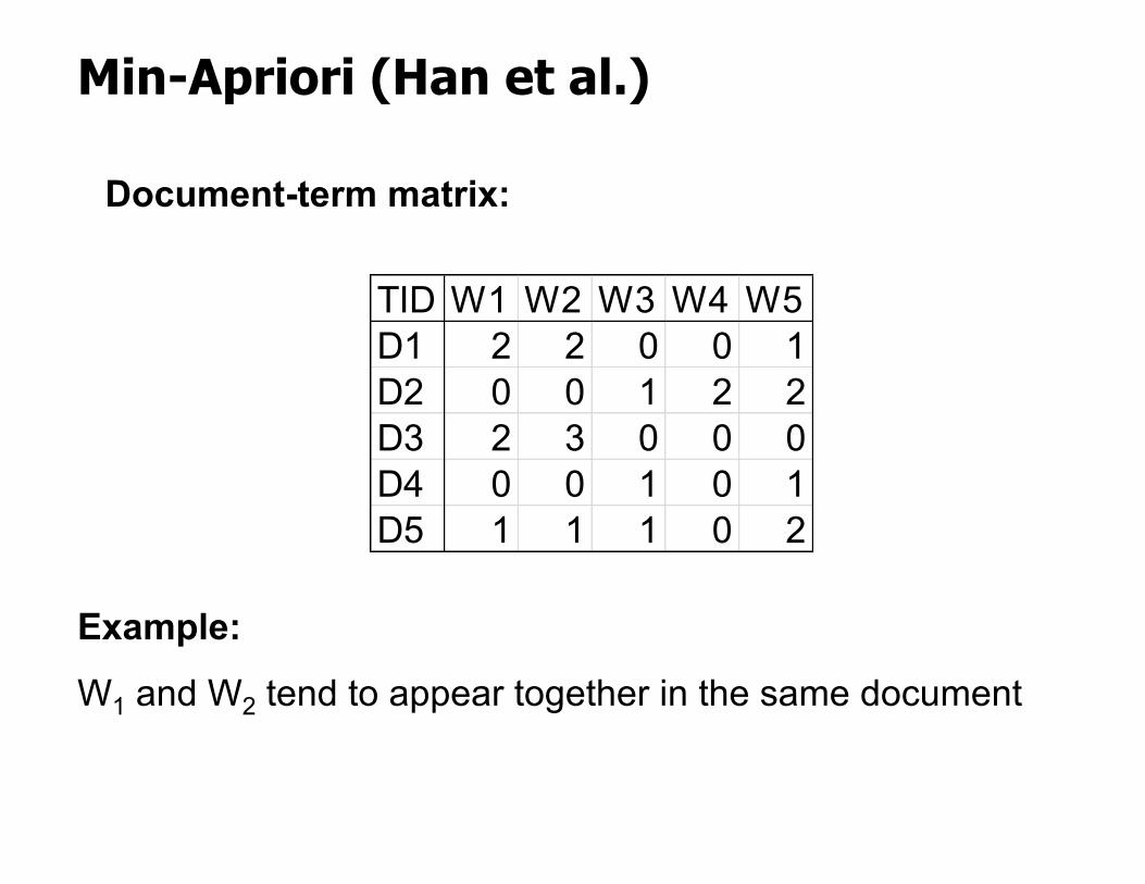
TID W1 W2 W3 W4 W5D1 2 2 0 0 1D2 0 0 1 2 2D3 2 3 0 0 0D4 0 0 1 0 1D5 1 1 1 0 2
Example:
W1 and W2 tend to appear together in the same document
Document-term matrix:
Min-Apriori
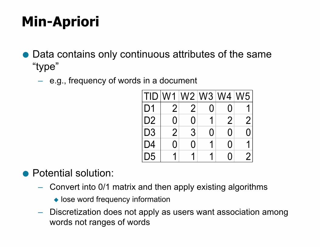
● Data contains only continuous attributes of the same “type”
– e.g., frequency of words in a document
● Potential solution:– Convert into 0/1 matrix and then apply existing algorithms
u lose word frequency information– Discretization does not apply as users want association among
words not ranges of words
TID W1 W2 W3 W4 W5D1 2 2 0 0 1D2 0 0 1 2 2D3 2 3 0 0 0D4 0 0 1 0 1D5 1 1 1 0 2
Min-Apriori
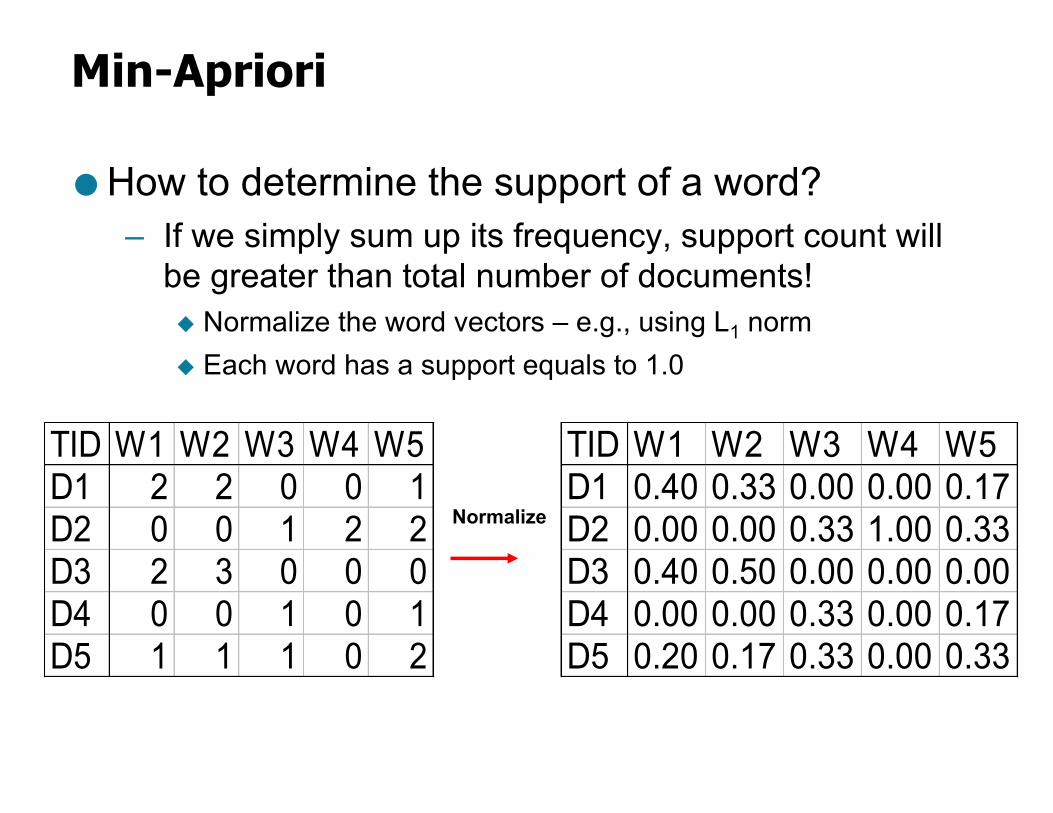
● How to determine the support of a word?– If we simply sum up its frequency, support count will
be greater than total number of documents!u Normalize the word vectors – e.g., using L1 normu Each word has a support equals to 1.0
TID W1 W2 W3 W4 W5D1 2 2 0 0 1D2 0 0 1 2 2D3 2 3 0 0 0D4 0 0 1 0 1D5 1 1 1 0 2
TID W1 W2 W3 W4 W5D1 0.40 0.33 0.00 0.00 0.17D2 0.00 0.00 0.33 1.00 0.33D3 0.40 0.50 0.00 0.00 0.00D4 0.00 0.00 0.33 0.00 0.17D5 0.20 0.17 0.33 0.00 0.33
Normalize
Min-Apriori
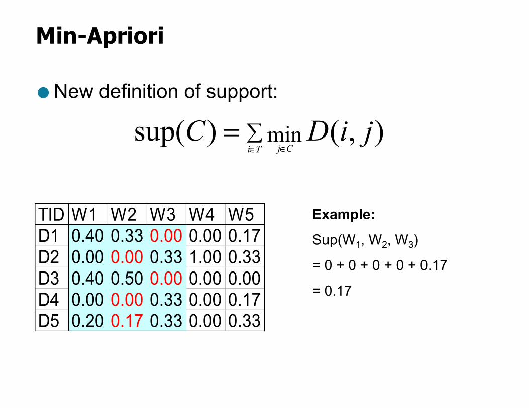
● New definition of support:
åÎ Î
=Ti Cj
jiDC ),()sup( min
Example:
Sup(W1, W2, W3)
= 0 + 0 + 0 + 0 + 0.17
= 0.17
TID W1 W2 W3 W4 W5D1 0.40 0.33 0.00 0.00 0.17D2 0.00 0.00 0.33 1.00 0.33D3 0.40 0.50 0.00 0.00 0.00D4 0.00 0.00 0.33 0.00 0.17D5 0.20 0.17 0.33 0.00 0.33
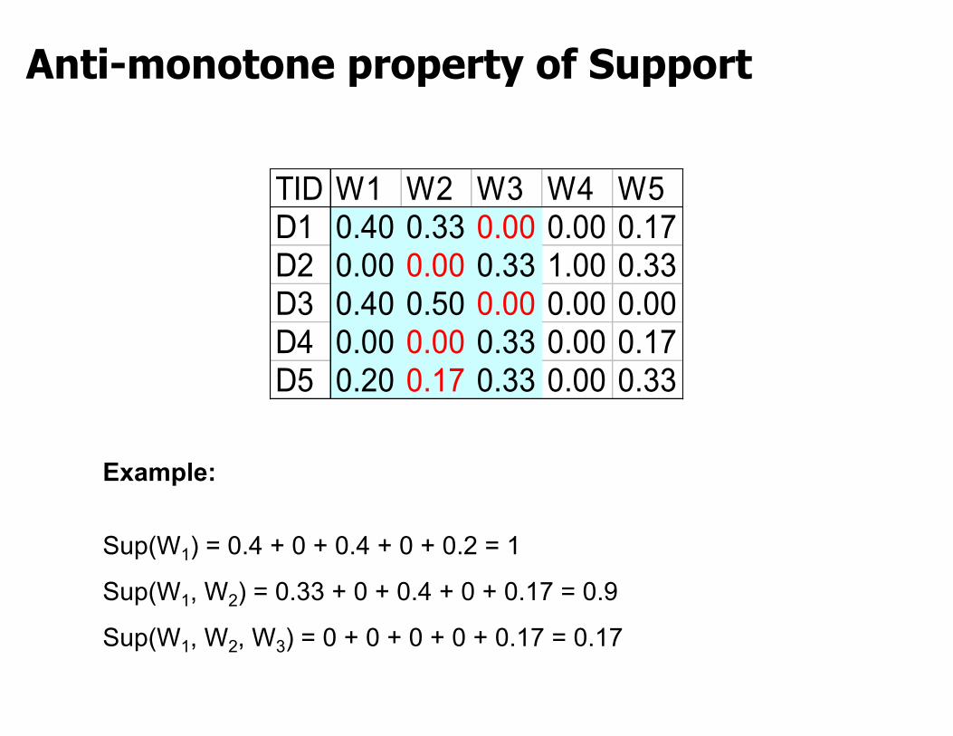
Anti-monotone property of Support
Example:
Sup(W1) = 0.4 + 0 + 0.4 + 0 + 0.2 = 1
Sup(W1, W2) = 0.33 + 0 + 0.4 + 0 + 0.17 = 0.9
Sup(W1, W2, W3) = 0 + 0 + 0 + 0 + 0.17 = 0.17
TID W1 W2 W3 W4 W5D1 0.40 0.33 0.00 0.00 0.17D2 0.00 0.00 0.33 1.00 0.33D3 0.40 0.50 0.00 0.00 0.00D4 0.00 0.00 0.33 0.00 0.17D5 0.20 0.17 0.33 0.00 0.33
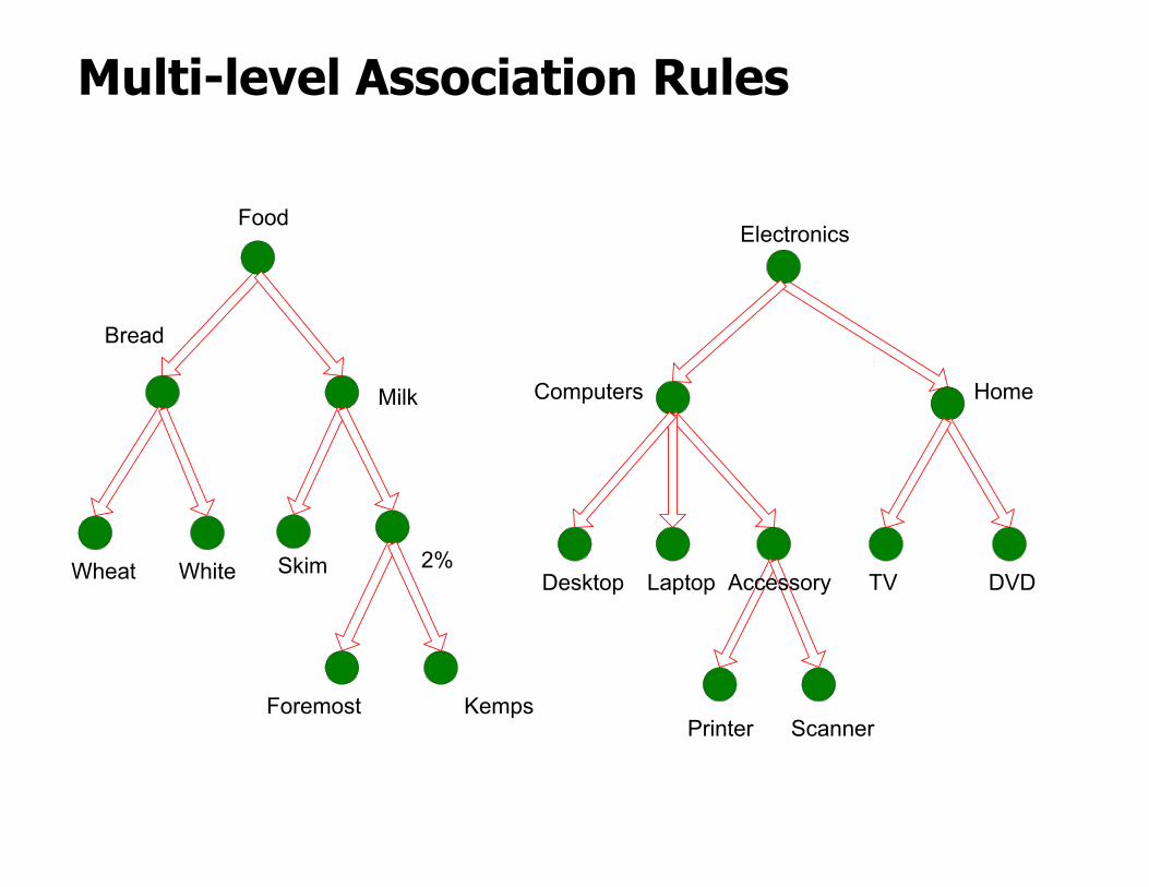
Multi-level Association Rules
Food
Bread
Milk
Skim 2%
Electronics
Computers Home
Desktop LaptopWheat White
Foremost Kemps
DVDTV
Printer Scanner
Accessory
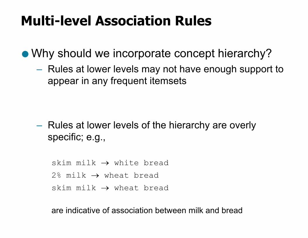
Multi-level Association Rules
● Why should we incorporate concept hierarchy?– Rules at lower levels may not have enough support to
appear in any frequent itemsets
– Rules at lower levels of the hierarchy are overly specific; e.g.,
skim milk ® white bread2% milk ® wheat breadskim milk ® wheat bread
are indicative of association between milk and bread
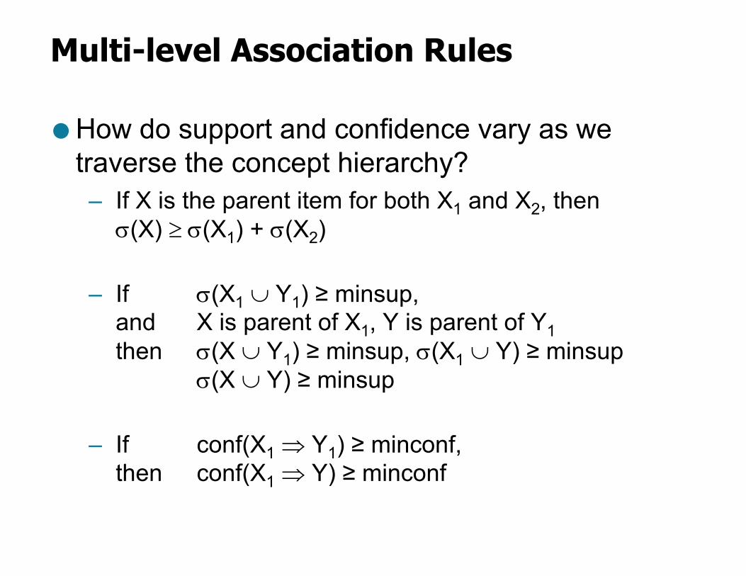
Multi-level Association Rules
● How do support and confidence vary as we traverse the concept hierarchy?– If X is the parent item for both X1 and X2, then s(X) ³ s(X1) + s(X2)
– If s(X1 È Y1) ≥ minsup, and X is parent of X1, Y is parent of Y1then s(X È Y1) ≥ minsup, s(X1 È Y) ≥ minsup
s(X È Y) ≥ minsup
– If conf(X1 Þ Y1) ≥ minconf,then conf(X1 Þ Y) ≥ minconf
Multi-level Association Rules
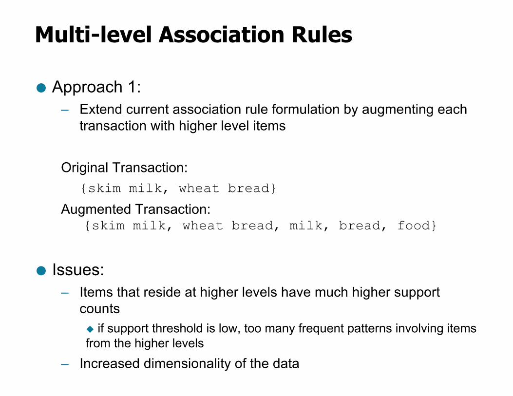
● Approach 1:– Extend current association rule formulation by augmenting each
transaction with higher level items
Original Transaction: {skim milk, wheat bread}
Augmented Transaction:{skim milk, wheat bread, milk, bread, food}
● Issues:– Items that reside at higher levels have much higher support
counts u if support threshold is low, too many frequent patterns involving items from the higher levels
– Increased dimensionality of the data
Multi-level Association Rules
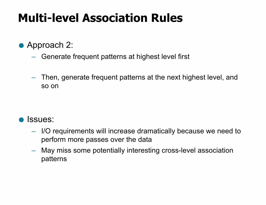
● Approach 2:– Generate frequent patterns at highest level first
– Then, generate frequent patterns at the next highest level, and so on
● Issues:– I/O requirements will increase dramatically because we need to
perform more passes over the data– May miss some potentially interesting cross-level association
patterns
Sequential Patterns
10 15 20 25 30 35
235
61
1
Timeline
Object A:
Object B:
Object C:
456
2 7812
16
178
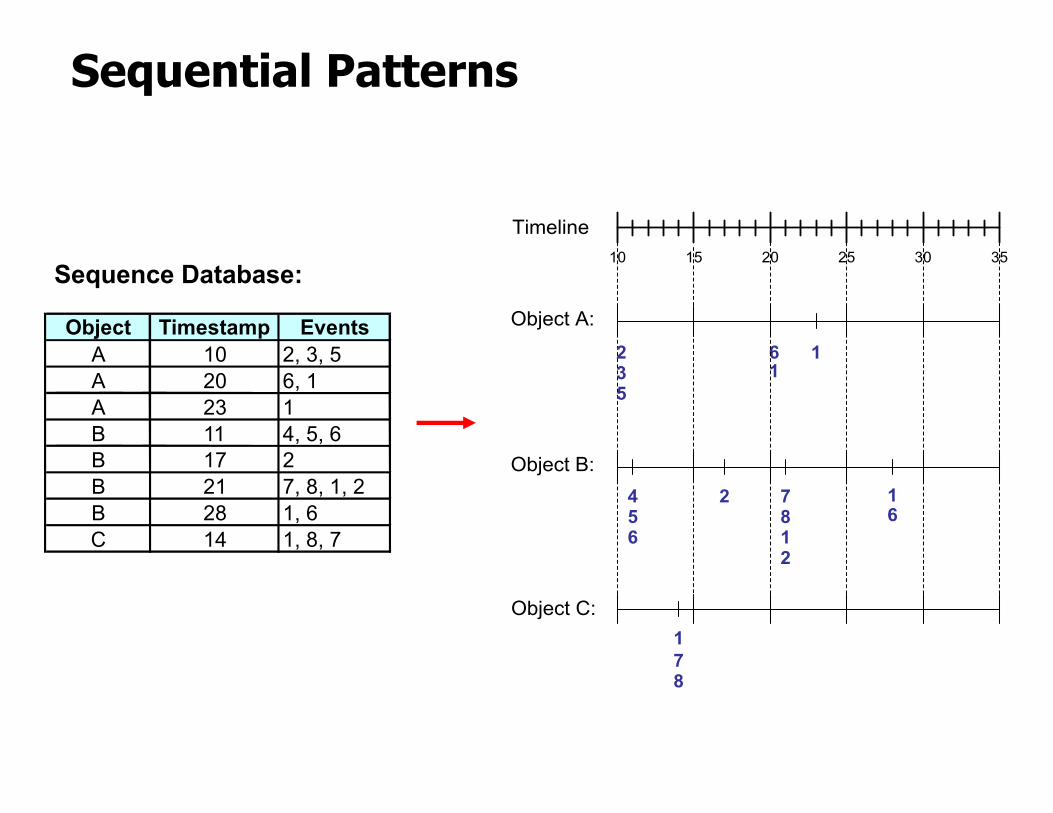
Object Timestamp EventsA 10 2, 3, 5A 20 6, 1A 23 1B 11 4, 5, 6B 17 2B 21 7, 8, 1, 2B 28 1, 6C 14 1, 8, 7
Sequence Database:
Examples of Sequence Data
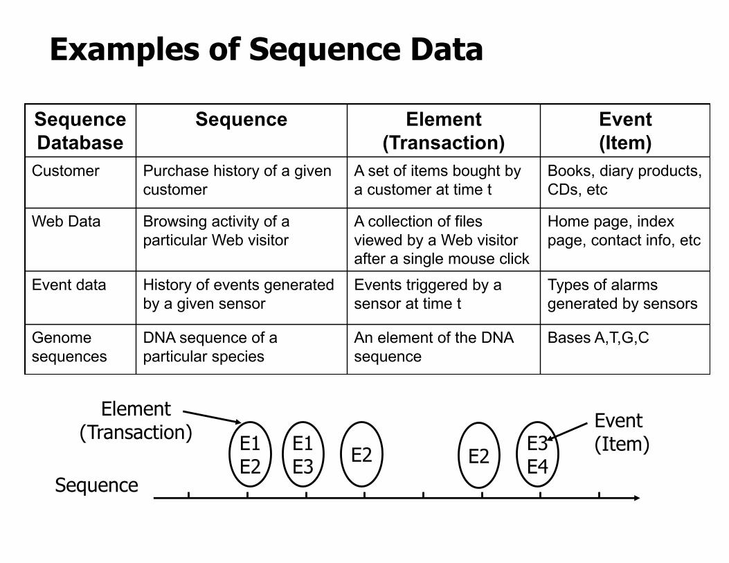
Sequence Database
Sequence Element (Transaction)
Event(Item)
Customer Purchase history of a given customer
A set of items bought by a customer at time t
Books, diary products, CDs, etc
Web Data Browsing activity of a particular Web visitor
A collection of files viewed by a Web visitor after a single mouse click
Home page, index page, contact info, etc
Event data History of events generated by a given sensor
Events triggered by a sensor at time t
Types of alarms generated by sensors
Genome sequences
DNA sequence of a particular species
An element of the DNA sequence
Bases A,T,G,C
Sequence
E1E2
E1E3 E2 E3
E4E2
Element (Transaction) Event
(Item)
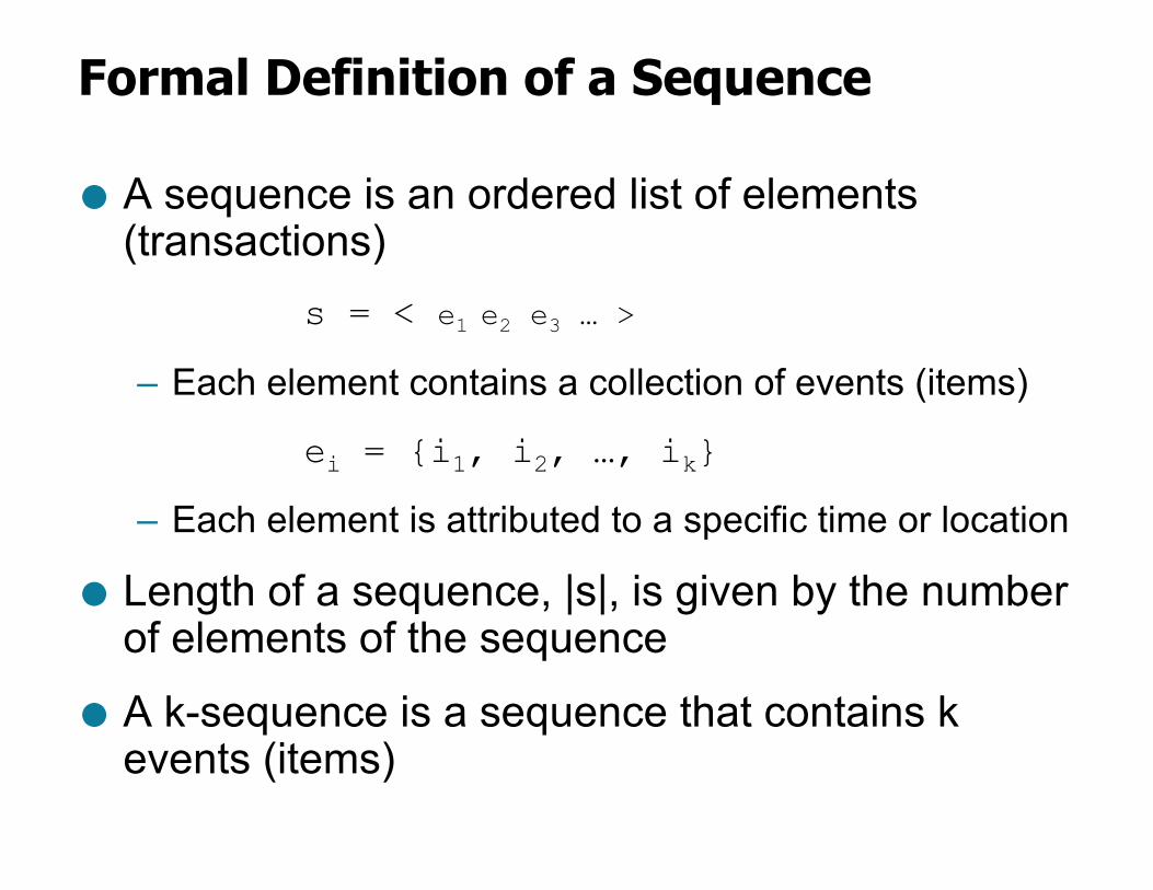
Formal Definition of a Sequence
● A sequence is an ordered list of elements (transactions)
s = < e1 e2 e3 … >
– Each element contains a collection of events (items)
ei = {i1, i2, …, ik}
– Each element is attributed to a specific time or location
● Length of a sequence, |s|, is given by the number of elements of the sequence
● A k-sequence is a sequence that contains k events (items)
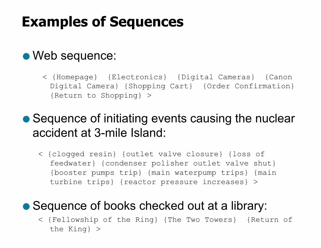
Examples of Sequences
● Web sequence:< {Homepage} {Electronics} {Digital Cameras} {Canon Digital Camera} {Shopping Cart} {Order Confirmation} {Return to Shopping} >
● Sequence of initiating events causing the nuclear accident at 3-mile Island:< {clogged resin} {outlet valve closure} {loss of
feedwater} {condenser polisher outlet valve shut} {booster pumps trip} {main waterpump trips} {main turbine trips} {reactor pressure increases} >
● Sequence of books checked out at a library:< {Fellowship of the Ring} {The Two Towers} {Return of
the King} >
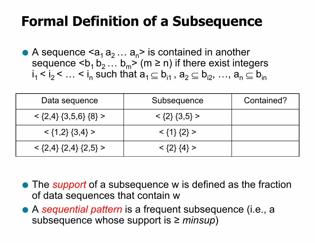
Formal Definition of a Subsequence
● A sequence <a1 a2 … an> is contained in another sequence <b1 b2 … bm> (m ≥ n) if there exist integers i1 < i2 < … < in such that a1 Í bi1 , a2 Í bi2, …, an Í bin
● The support of a subsequence w is defined as the fraction of data sequences that contain w
● A sequential pattern is a frequent subsequence (i.e., a subsequence whose support is ≥ minsup)
Data sequence Subsequence Contained?
< {2,4} {3,5,6} {8} > < {2} {3,5} >
< {1,2} {3,4} > < {1} {2} >
< {2,4} {2,4} {2,5} > < {2} {4} >
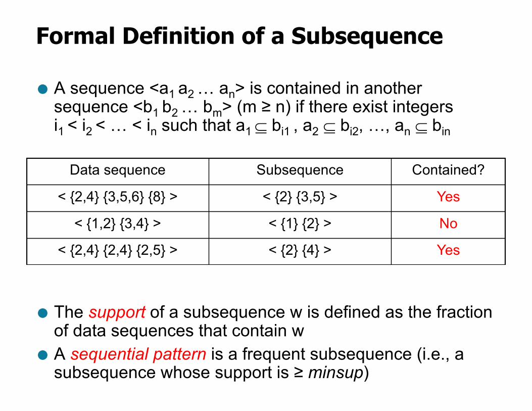
Formal Definition of a Subsequence
● A sequence <a1 a2 … an> is contained in another sequence <b1 b2 … bm> (m ≥ n) if there exist integers i1 < i2 < … < in such that a1 Í bi1 , a2 Í bi2, …, an Í bin
● The support of a subsequence w is defined as the fraction of data sequences that contain w
● A sequential pattern is a frequent subsequence (i.e., a subsequence whose support is ≥ minsup)
Data sequence Subsequence Contained?
< {2,4} {3,5,6} {8} > < {2} {3,5} > Yes
< {1,2} {3,4} > < {1} {2} > No
< {2,4} {2,4} {2,5} > < {2} {4} > Yes
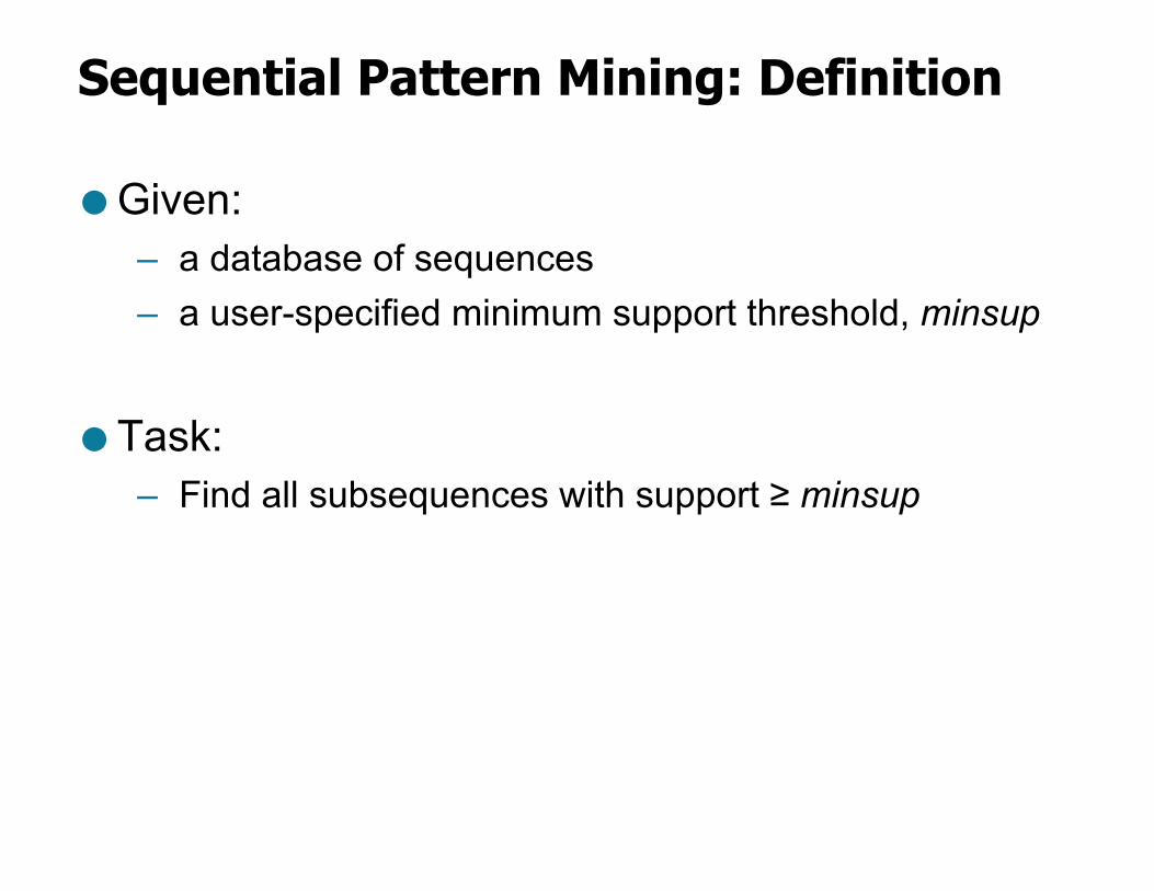
Sequential Pattern Mining: Definition
● Given: – a database of sequences – a user-specified minimum support threshold, minsup
● Task:– Find all subsequences with support ≥ minsup
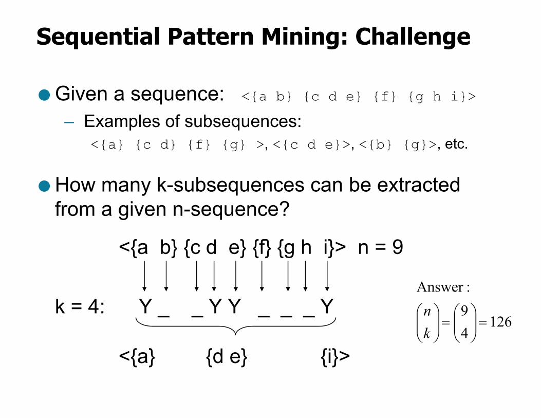
Sequential Pattern Mining: Challenge
● Given a sequence: <{a b} {c d e} {f} {g h i}>– Examples of subsequences:
<{a} {c d} {f} {g} >, <{c d e}>, <{b} {g}>, etc.
● How many k-subsequences can be extracted from a given n-sequence?
<{a b} {c d e} {f} {g h i}> n = 9
k = 4: Y _ _ Y Y _ _ _ Y
<{a} {d e} {i}>
12649:Answer
=÷÷ø
öççè
æ=÷÷
ø
öççè
ækn
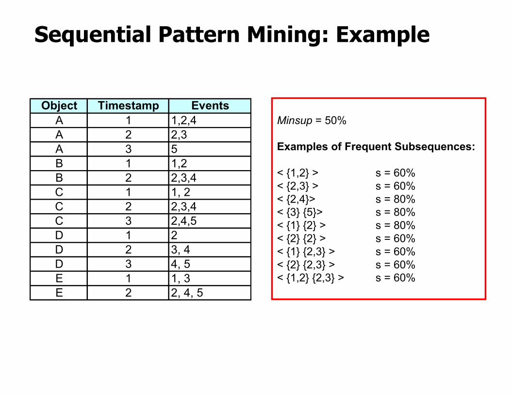
Sequential Pattern Mining: Example
Minsup = 50%
Examples of Frequent Subsequences:
< {1,2} > s = 60%< {2,3} > s = 60%< {2,4}> s = 80%< {3} {5}> s = 80%< {1} {2} > s = 80%< {2} {2} > s = 60%< {1} {2,3} > s = 60%< {2} {2,3} > s = 60%< {1,2} {2,3} > s = 60%
Object Timestamp EventsA 1 1,2,4A 2 2,3A 3 5B 1 1,2B 2 2,3,4C 1 1, 2C 2 2,3,4C 3 2,4,5D 1 2D 2 3, 4D 3 4, 5E 1 1, 3E 2 2, 4, 5
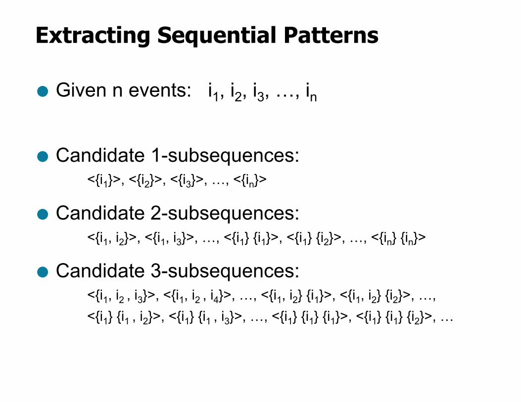
Extracting Sequential Patterns
● Given n events: i1, i2, i3, …, in
● Candidate 1-subsequences: <{i1}>, <{i2}>, <{i3}>, …, <{in}>
● Candidate 2-subsequences:<{i1, i2}>, <{i1, i3}>, …, <{i1} {i1}>, <{i1} {i2}>, …, <{in} {in}>
● Candidate 3-subsequences:<{i1, i2 , i3}>, <{i1, i2 , i4}>, …, <{i1, i2} {i1}>, <{i1, i2} {i2}>, …,<{i1} {i1 , i2}>, <{i1} {i1 , i3}>, …, <{i1} {i1} {i1}>, <{i1} {i1} {i2}>, …
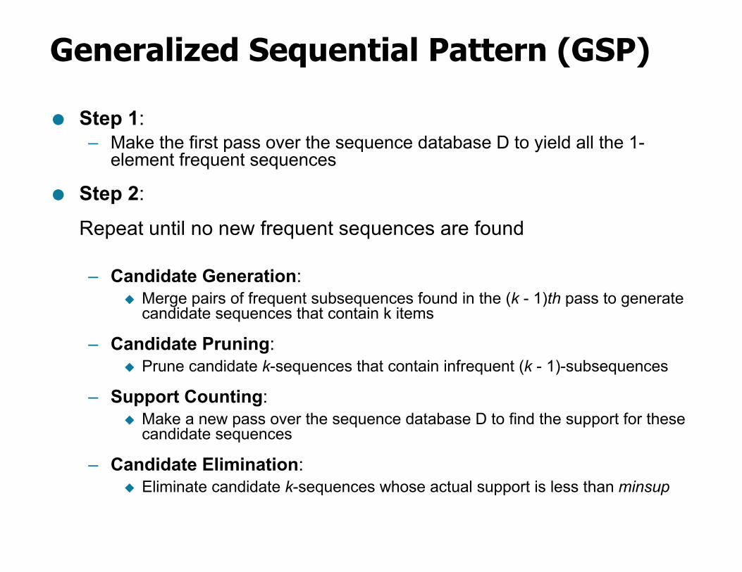
Generalized Sequential Pattern (GSP)
● Step 1: – Make the first pass over the sequence database D to yield all the 1-
element frequent sequences
● Step 2:
Repeat until no new frequent sequences are found
– Candidate Generation: u Merge pairs of frequent subsequences found in the (k - 1)th pass to generate
candidate sequences that contain k items
– Candidate Pruning:u Prune candidate k-sequences that contain infrequent (k - 1)-subsequences
– Support Counting:u Make a new pass over the sequence database D to find the support for these
candidate sequences
– Candidate Elimination:u Eliminate candidate k-sequences whose actual support is less than minsup
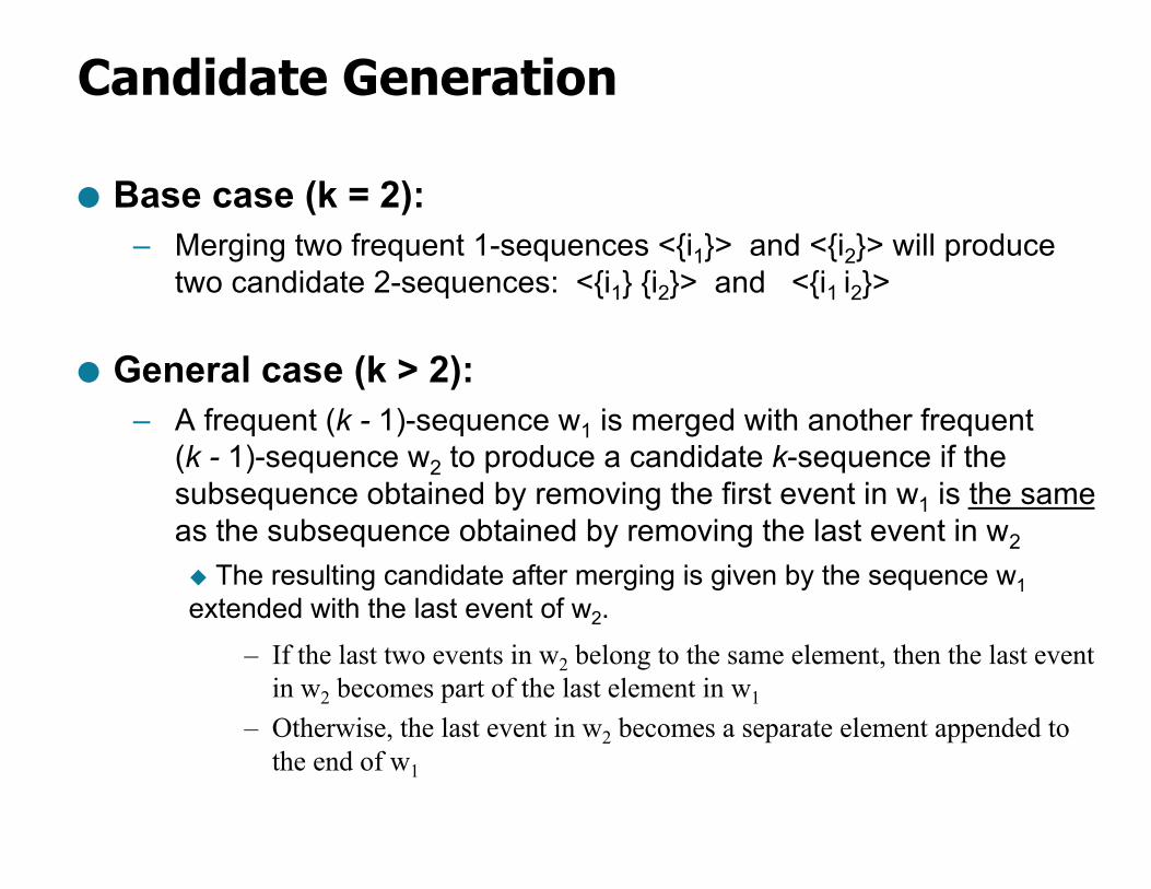
Candidate Generation
● Base case (k = 2):– Merging two frequent 1-sequences <{i1}> and <{i2}> will produce
two candidate 2-sequences: <{i1} {i2}> and <{i1 i2}>
● General case (k > 2):– A frequent (k - 1)-sequence w1 is merged with another frequent
(k - 1)-sequence w2 to produce a candidate k-sequence if the subsequence obtained by removing the first event in w1 is the same as the subsequence obtained by removing the last event in w2
u The resulting candidate after merging is given by the sequence w1extended with the last event of w2.
– If the last two events in w2 belong to the same element, then the last event in w2 becomes part of the last element in w1
– Otherwise, the last event in w2 becomes a separate element appended to the end of w1
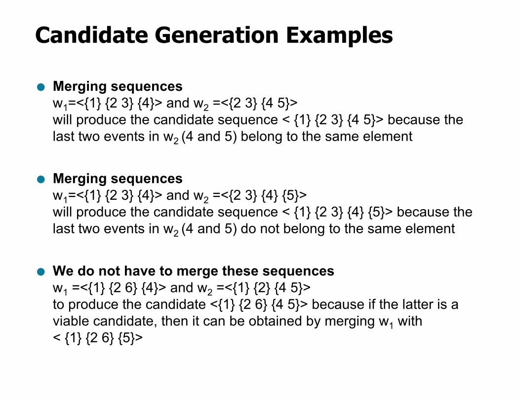
Candidate Generation Examples
● Merging sequencesw1=<{1} {2 3} {4}> and w2 =<{2 3} {4 5}> will produce the candidate sequence < {1} {2 3} {4 5}> because the last two events in w2 (4 and 5) belong to the same element
● Merging sequencesw1=<{1} {2 3} {4}> and w2 =<{2 3} {4} {5}> will produce the candidate sequence < {1} {2 3} {4} {5}> because the last two events in w2 (4 and 5) do not belong to the same element
● We do not have to merge these sequencesw1 =<{1} {2 6} {4}> and w2 =<{1} {2} {4 5}> to produce the candidate <{1} {2 6} {4 5}> because if the latter is a viable candidate, then it can be obtained by merging w1 with < {1} {2 6} {5}>
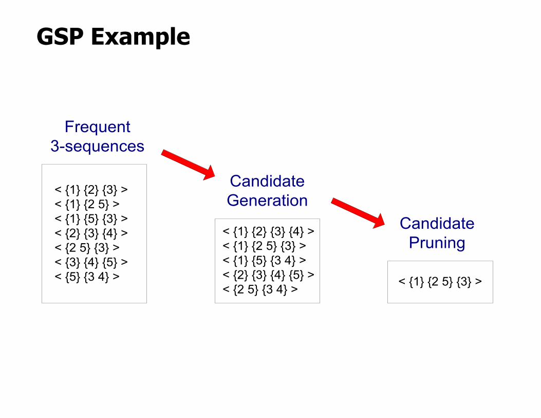
GSP Example
< {1} {2} {3} >< {1} {2 5} >< {1} {5} {3} >< {2} {3} {4} >< {2 5} {3} >< {3} {4} {5} >< {5} {3 4} >
< {1} {2} {3} {4} >< {1} {2 5} {3} >< {1} {5} {3 4} >< {2} {3} {4} {5} >< {2 5} {3 4} > < {1} {2 5} {3} >
Frequent3-sequences
CandidateGeneration
CandidatePruning
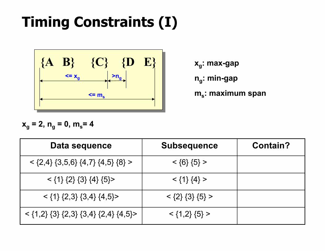
Timing Constraints (I)
{A B} {C} {D E}
<= ms
<= xg >ng
xg: max-gap
ng: min-gap
ms: maximum span
Data sequence Subsequence Contain?
< {2,4} {3,5,6} {4,7} {4,5} {8} > < {6} {5} >
< {1} {2} {3} {4} {5}> < {1} {4} >
< {1} {2,3} {3,4} {4,5}> < {2} {3} {5} >
< {1,2} {3} {2,3} {3,4} {2,4} {4,5}> < {1,2} {5} >
xg = 2, ng = 0, ms= 4

Timing Constraints (I)
{A B} {C} {D E}
<= ms
<= xg >ng
xg: max-gap
ng: min-gap
ms: maximum span
Data sequence Subsequence Contain?
< {2,4} {3,5,6} {4,7} {4,5} {8} > < {6} {5} > Yes
< {1} {2} {3} {4} {5}> < {1} {4} > No
< {1} {2,3} {3,4} {4,5}> < {2} {3} {5} > Yes
< {1,2} {3} {2,3} {3,4} {2,4} {4,5}> < {1,2} {5} > No
xg = 2, ng = 0, ms= 4
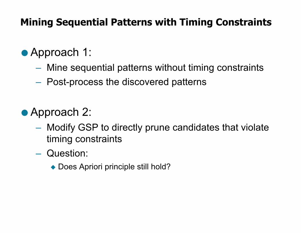
Mining Sequential Patterns with Timing Constraints
● Approach 1:– Mine sequential patterns without timing constraints– Post-process the discovered patterns
● Approach 2:– Modify GSP to directly prune candidates that violate
timing constraints– Question:
u Does Apriori principle still hold?
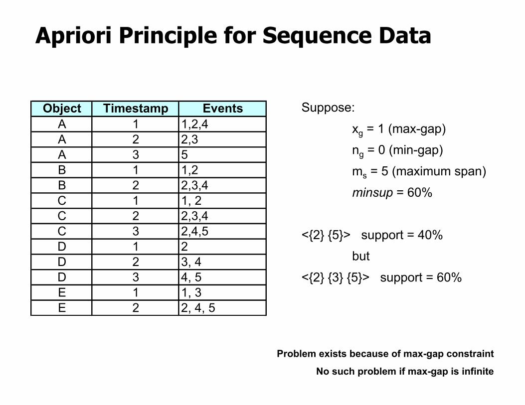
Apriori Principle for Sequence Data
Object Timestamp EventsA 1 1,2,4A 2 2,3A 3 5B 1 1,2B 2 2,3,4C 1 1, 2C 2 2,3,4C 3 2,4,5D 1 2D 2 3, 4D 3 4, 5E 1 1, 3E 2 2, 4, 5
Suppose: xg = 1 (max-gap)ng = 0 (min-gap)ms = 5 (maximum span)minsup = 60%
<{2} {5}> support = 40%but
<{2} {3} {5}> support = 60%
Problem exists because of max-gap constraint
No such problem if max-gap is infinite
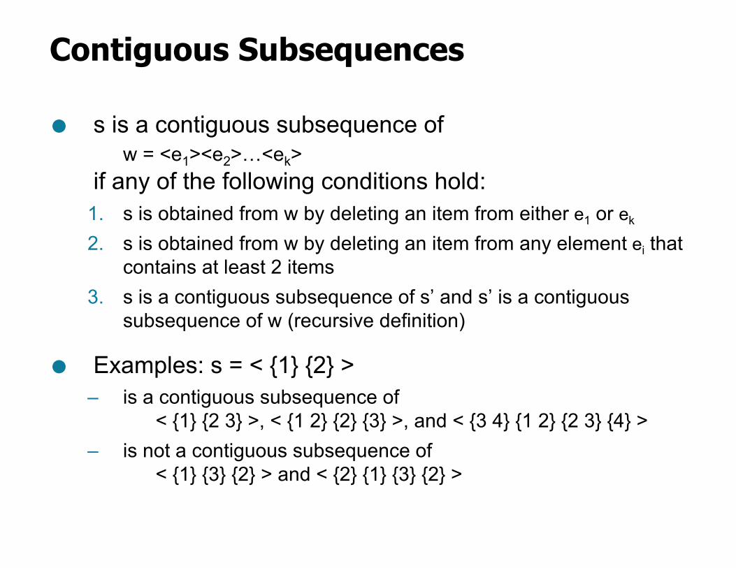
Contiguous Subsequences
● s is a contiguous subsequence of w = <e1><e2>…<ek>
if any of the following conditions hold:1. s is obtained from w by deleting an item from either e1 or ek
2. s is obtained from w by deleting an item from any element ei that contains at least 2 items
3. s is a contiguous subsequence of s’ and s’ is a contiguous subsequence of w (recursive definition)
● Examples: s = < {1} {2} > – is a contiguous subsequence of
< {1} {2 3} >, < {1 2} {2} {3} >, and < {3 4} {1 2} {2 3} {4} > – is not a contiguous subsequence of
< {1} {3} {2} > and < {2} {1} {3} {2} >
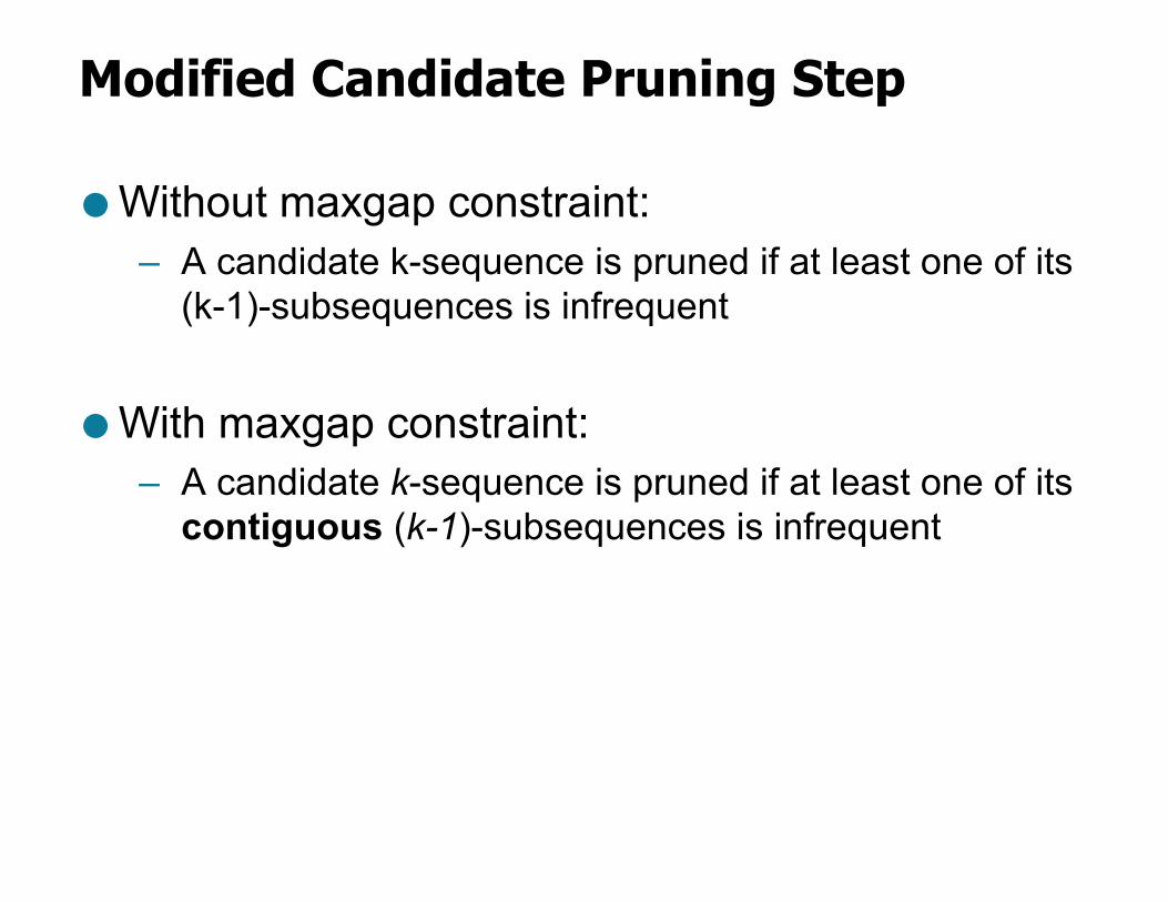
Modified Candidate Pruning Step
● Without maxgap constraint:– A candidate k-sequence is pruned if at least one of its
(k-1)-subsequences is infrequent
● With maxgap constraint:– A candidate k-sequence is pruned if at least one of its contiguous (k-1)-subsequences is infrequent
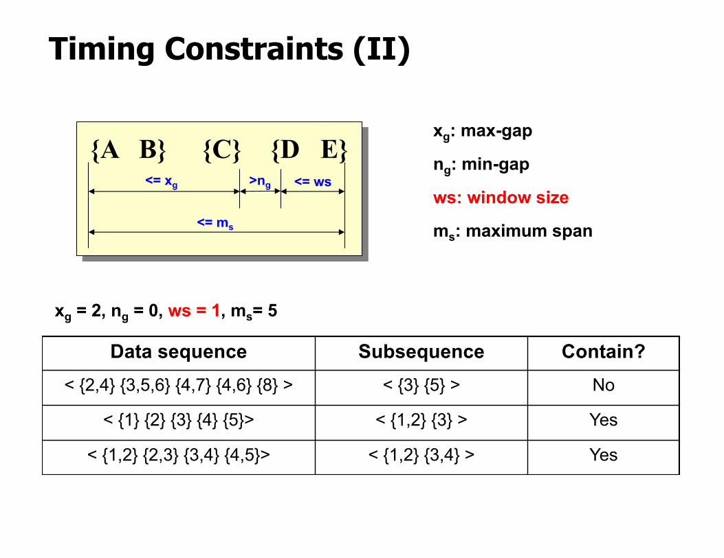
Timing Constraints (II)
{A B} {C} {D E}
<= ms
<= xg >ng <= ws
xg: max-gap
ng: min-gap
ws: window size
ms: maximum span
Data sequence Subsequence Contain?< {2,4} {3,5,6} {4,7} {4,6} {8} > < {3} {5} > No
< {1} {2} {3} {4} {5}> < {1,2} {3} > Yes
< {1,2} {2,3} {3,4} {4,5}> < {1,2} {3,4} > Yes
xg = 2, ng = 0, ws = 1, ms= 5
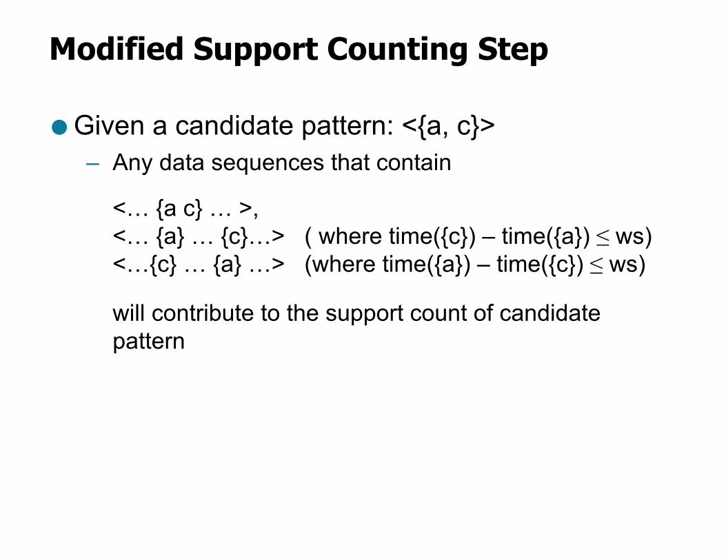
Modified Support Counting Step
● Given a candidate pattern: <{a, c}>– Any data sequences that contain
<… {a c} … >,<… {a} … {c}…> ( where time({c}) – time({a}) ≤ ws) <…{c} … {a} …> (where time({a}) – time({c}) ≤ ws)
will contribute to the support count of candidate pattern
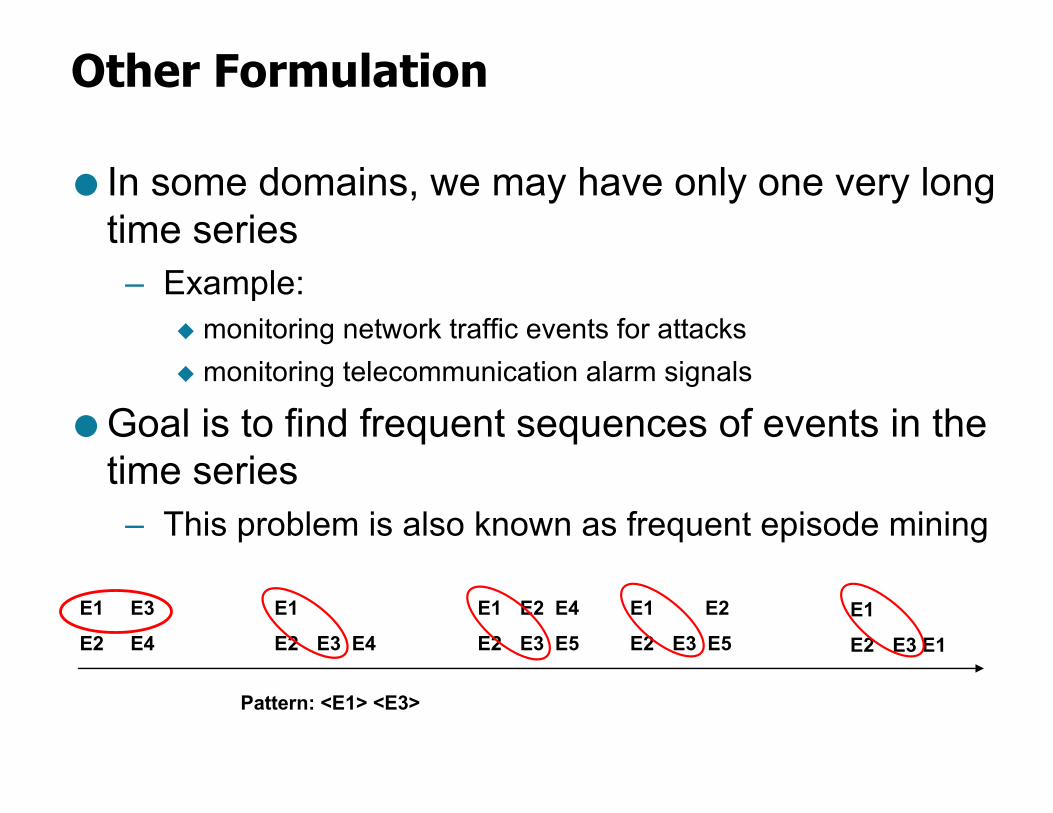
Other Formulation
● In some domains, we may have only one very long time series– Example:
u monitoring network traffic events for attacksu monitoring telecommunication alarm signals
● Goal is to find frequent sequences of events in the time series– This problem is also known as frequent episode mining
E1
E2
E1
E2
E1
E2
E3
E4 E3 E4
E1
E2
E2 E4
E3 E5
E2
E3 E5E1
E2 E3 E1
Pattern: <E1> <E3>
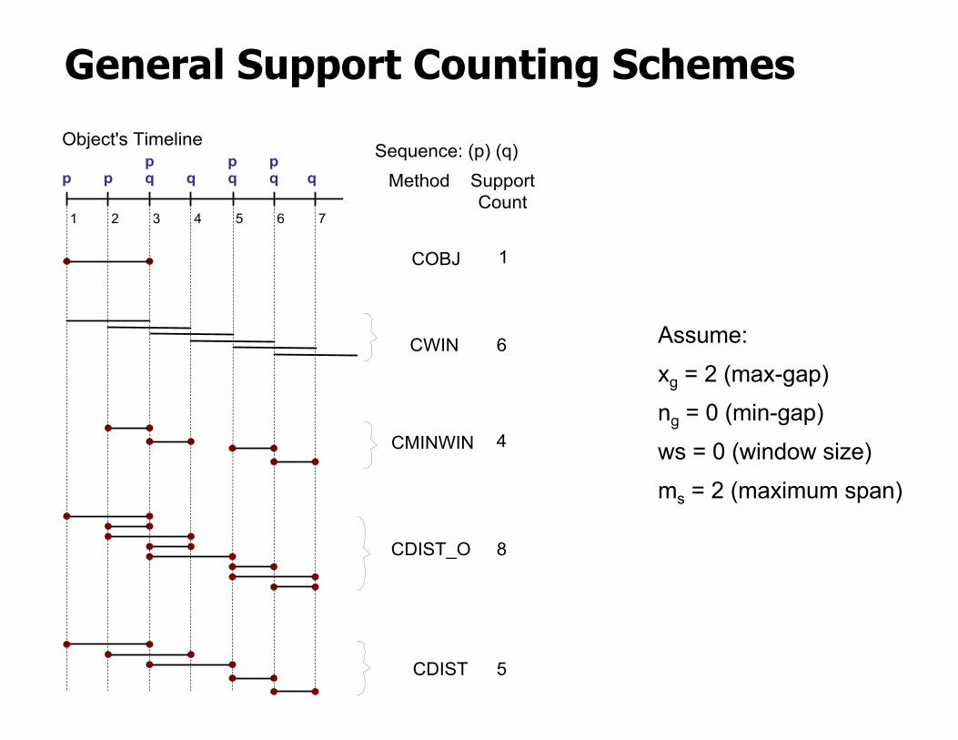
General Support Counting Schemes
p
Object's Timeline Sequence: (p) (q)Method Support Count
COBJ 1
1
CWIN 6
CMINWIN 4
p qp
q qp
qqp
2 3 4 5 6 7
CDIST_O 8
CDIST 5
Assume: xg = 2 (max-gap)ng = 0 (min-gap)ws = 0 (window size)ms = 2 (maximum span)
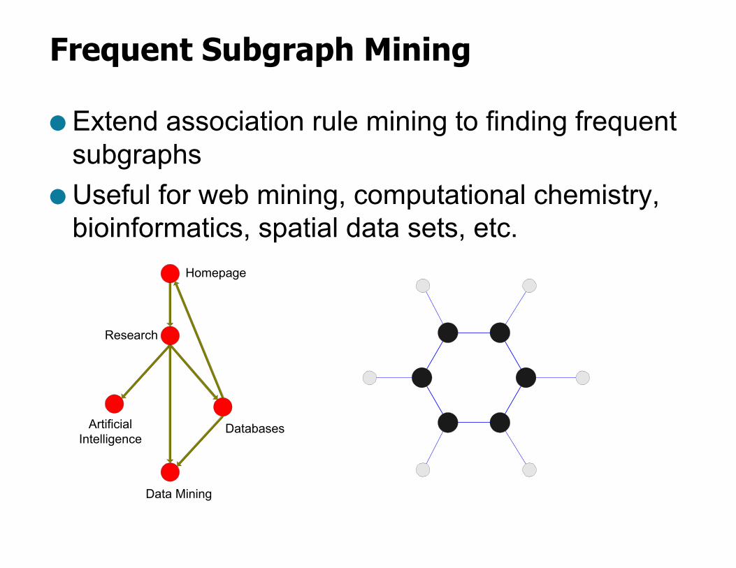
Frequent Subgraph Mining
● Extend association rule mining to finding frequent subgraphs
● Useful for web mining, computational chemistry, bioinformatics, spatial data sets, etc.
Databases
Homepage
Research
ArtificialIntelligence
Data Mining
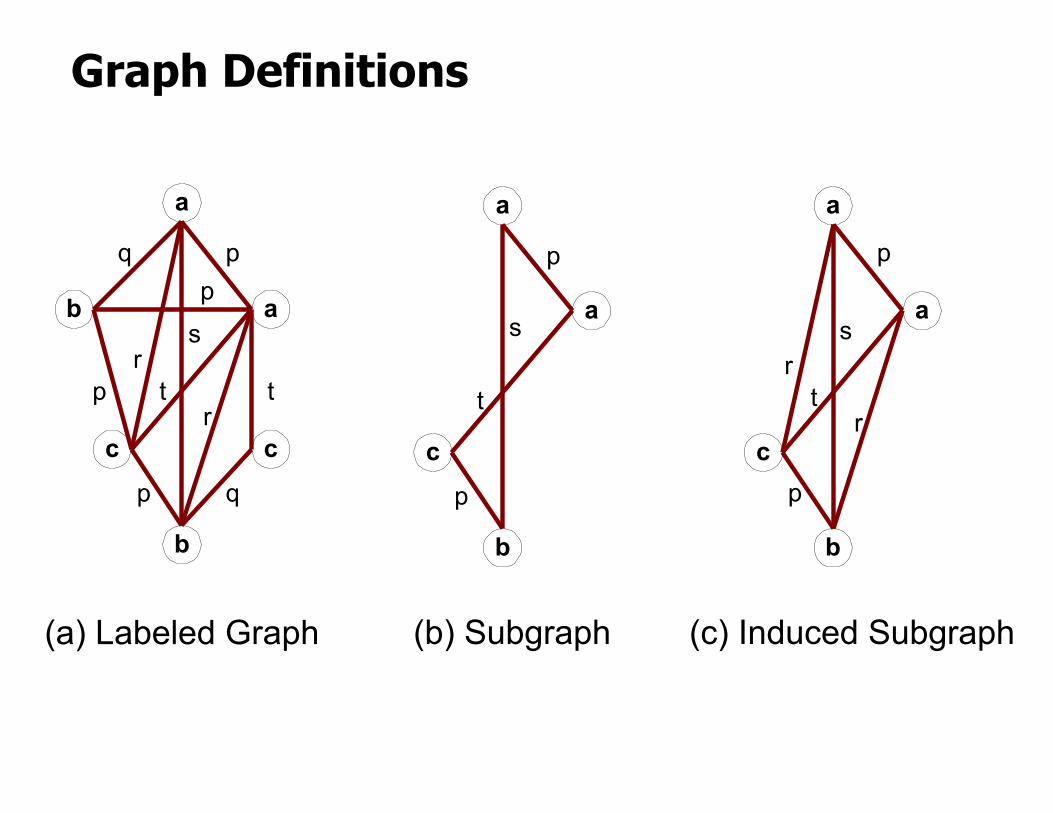
Graph Definitions
a
b a
c c
b
(a) Labeled Graph
pq
p
p
rs
tr
t
qp
a
a
c
b
(b) Subgraph
p
s
t
p
a
a
c
b
(c) Induced Subgraph
p
rs
tr
p
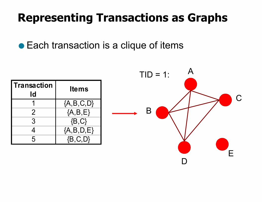
Representing Transactions as Graphs
● Each transaction is a clique of items
Transaction Id
Items
1 {A,B,C,D}2 {A,B,E}3 {B,C}4 {A,B,D,E}5 {B,C,D}
A
BC
DE
TID = 1:
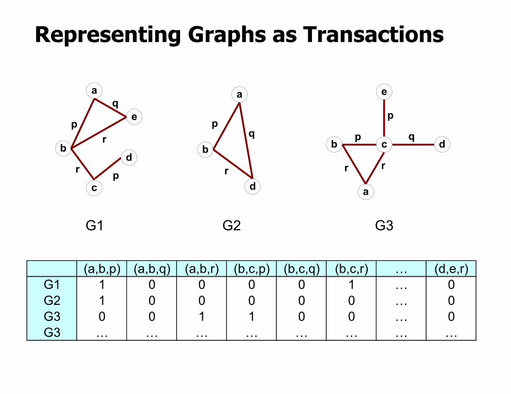
Representing Graphs as Transactions
a
b
e
c
p
q
r p
a
b
d
p
r
G1 G2
q
e
c
a
p q
r
b
p
G3
d
rd
r
(a,b,p) (a,b,q) (a,b,r) (b,c,p) (b,c,q) (b,c,r) … (d,e,r)G1 1 0 0 0 0 1 … 0G2 1 0 0 0 0 0 … 0G3 0 0 1 1 0 0 … 0G3 … … … … … … … …
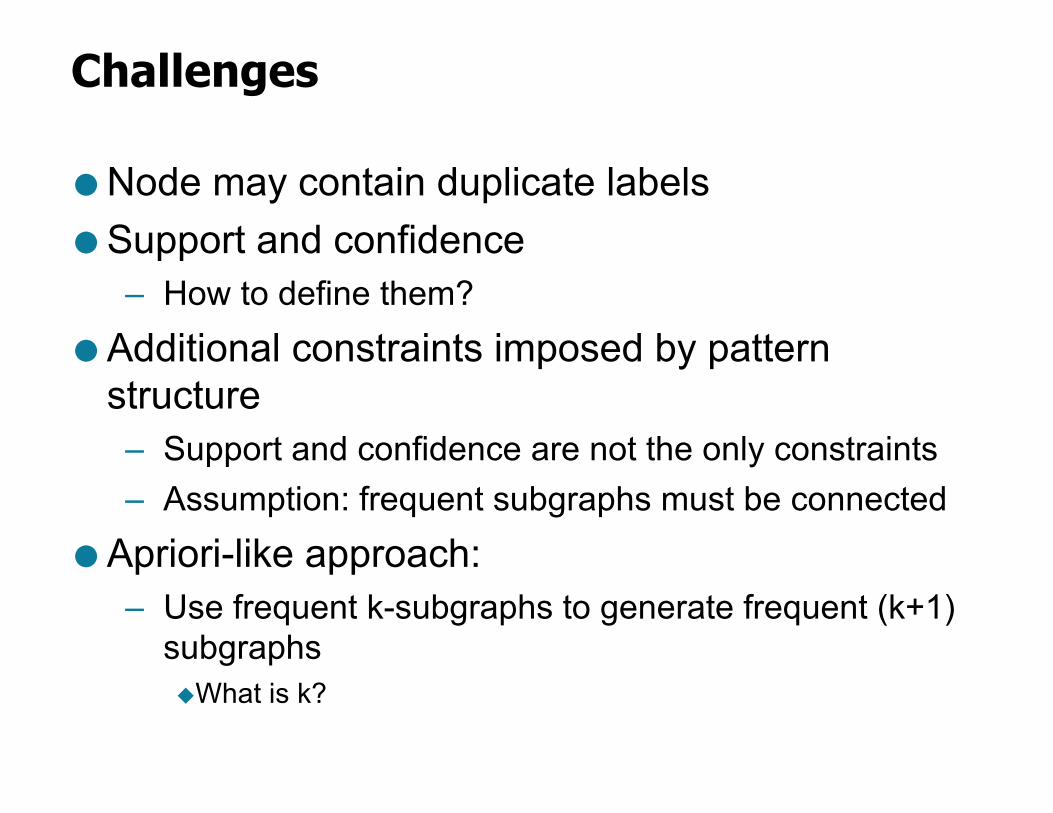
Challenges
● Node may contain duplicate labels● Support and confidence
– How to define them?● Additional constraints imposed by pattern
structure– Support and confidence are not the only constraints– Assumption: frequent subgraphs must be connected
● Apriori-like approach: – Use frequent k-subgraphs to generate frequent (k+1)
subgraphsuWhat is k?
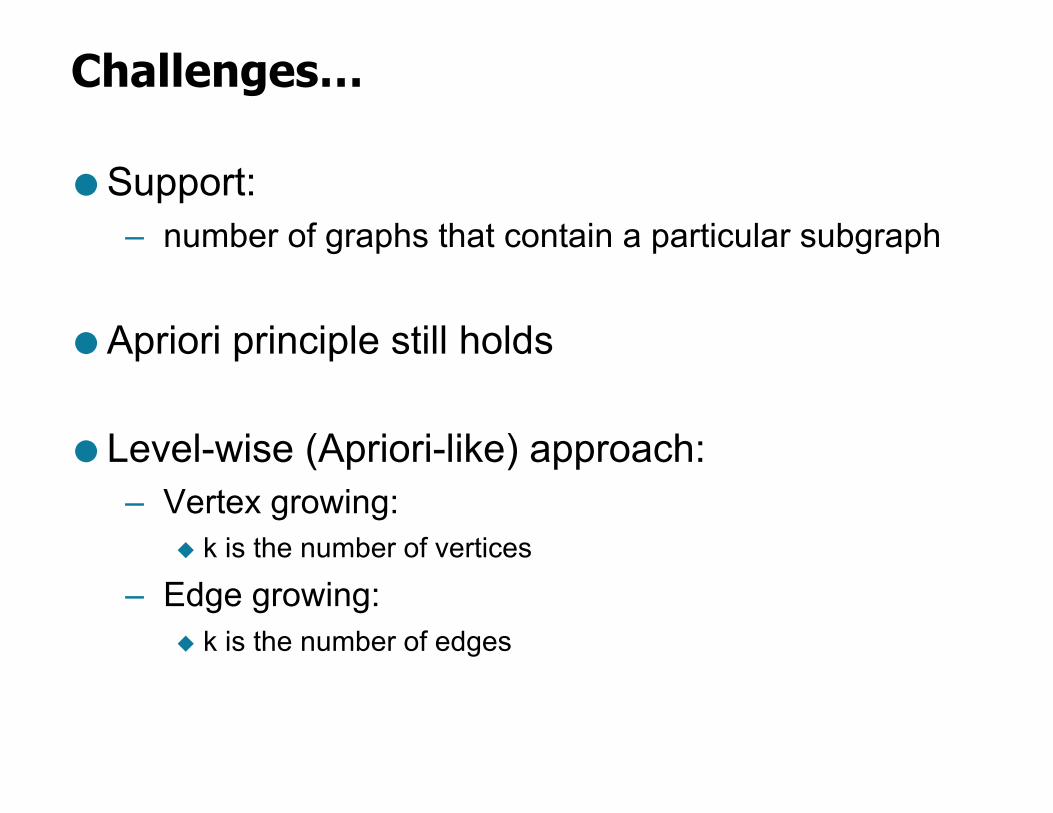
Challenges…
● Support: – number of graphs that contain a particular subgraph
● Apriori principle still holds
● Level-wise (Apriori-like) approach:– Vertex growing:
u k is the number of vertices
– Edge growing:u k is the number of edges
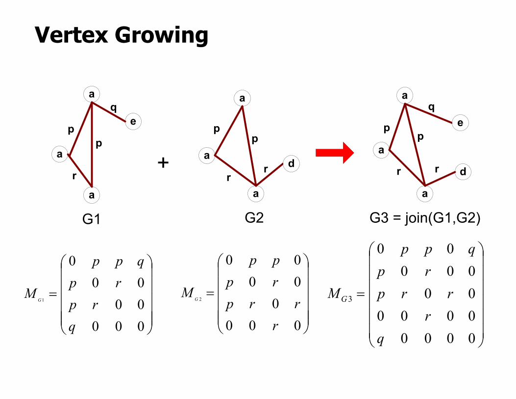
Vertex Growing
a
a
e
a
p
q
r
p
a
a
a
p
rr
d
G1 G2
p
÷÷÷÷÷
ø
ö
ççççç
è
æ
=
0000000
0
1
qrp
rpqpp
MG
÷÷÷÷÷
ø
ö
ççççç
è
æ
=
00000000
2
rrrp
rppp
MG
a
a
a
p
q
r
ep
÷÷÷÷÷÷
ø
ö
çççççç
è
æ
=
0000000000000
00
3
qrrrp
rpqpp
MG
G3 = join(G1,G2)
dr+
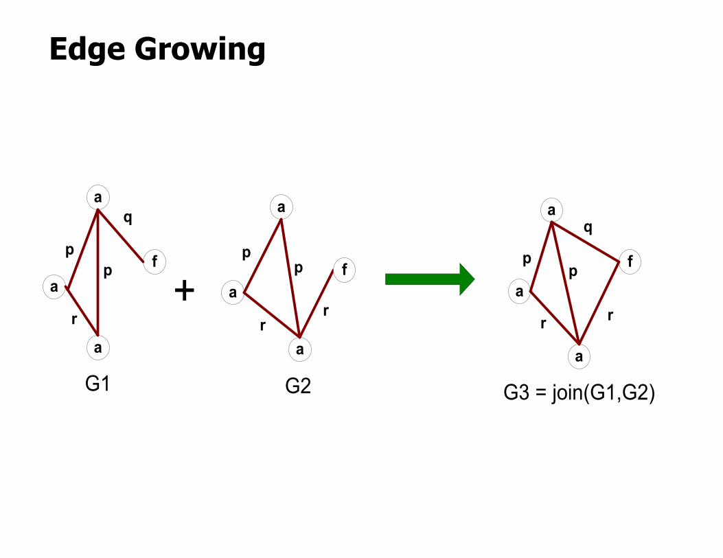
Edge Growing
a
af
a
p
q
r
p
a
a
a
p
rr
f
G1 G2
p
a
a
a
p
q
r
fp
G3 = join(G1,G2)
r+
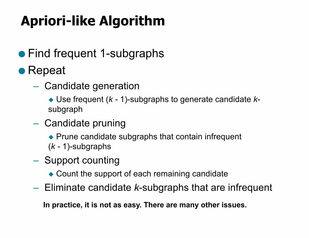
Apriori-like Algorithm
● Find frequent 1-subgraphs● Repeat
– Candidate generationu Use frequent (k - 1)-subgraphs to generate candidate k-subgraph
– Candidate pruningu Prune candidate subgraphs that contain infrequent (k - 1)-subgraphs
– Support countingu Count the support of each remaining candidate
– Eliminate candidate k-subgraphs that are infrequentIn practice, it is not as easy. There are many other issues.
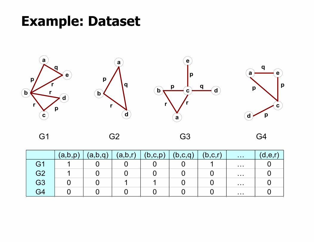
Example: Dataset
a
b
e
c
p
q
r p
a
b
d
p
r
G1 G2
q
e
c
a
p q
r
b
p
G3
d
rd
r
(a,b,p) (a,b,q) (a,b,r) (b,c,p) (b,c,q) (b,c,r) … (d,e,r)G1 1 0 0 0 0 1 … 0G2 1 0 0 0 0 0 … 0G3 0 0 1 1 0 0 … 0G4 0 0 0 0 0 0 … 0
a eq
cd
p p
p
G4
r
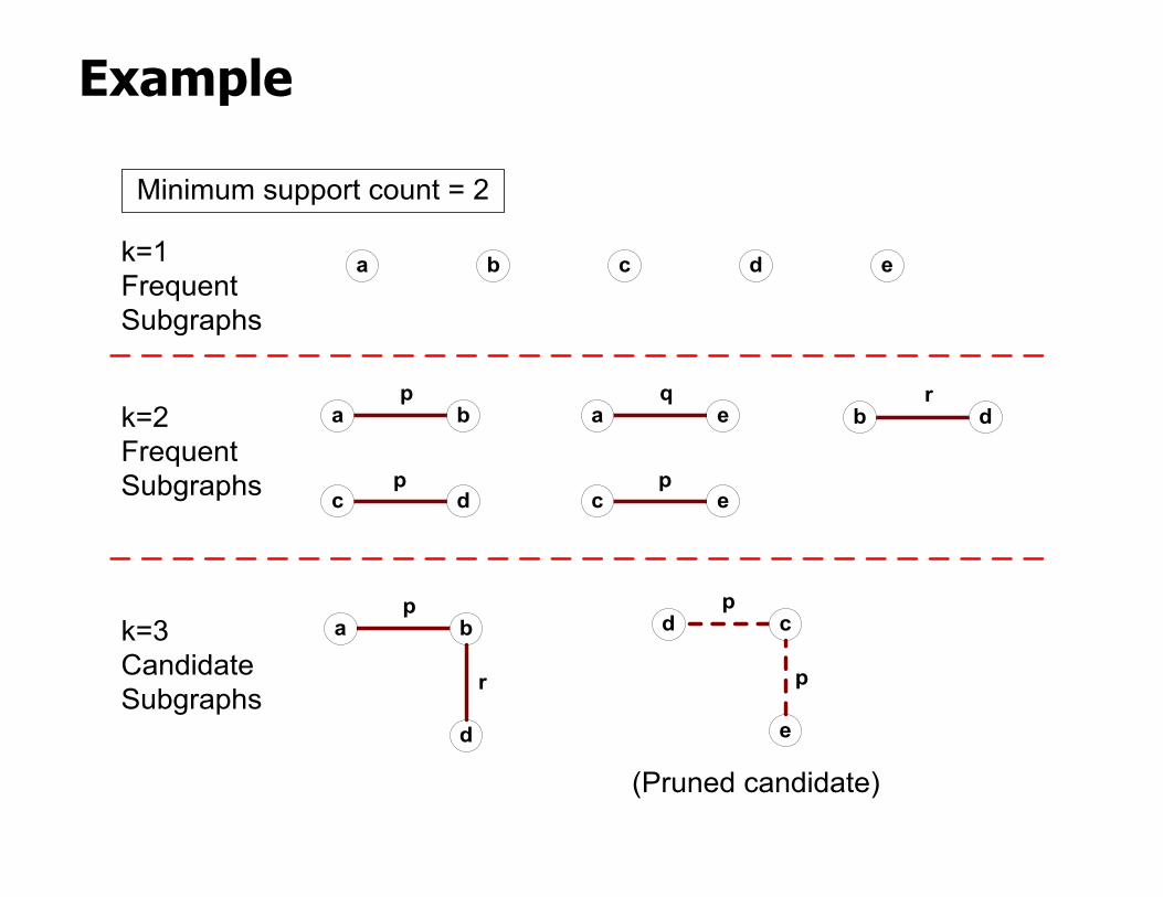
Example
p
a b c d ek=1FrequentSubgraphs
a b
pc d
pc e
qa e
rb d
pa b
d
r
pd c
e
p
(Pruned candidate)
Minimum support count = 2
k=2FrequentSubgraphs
k=3CandidateSubgraphs
Candidate Generation
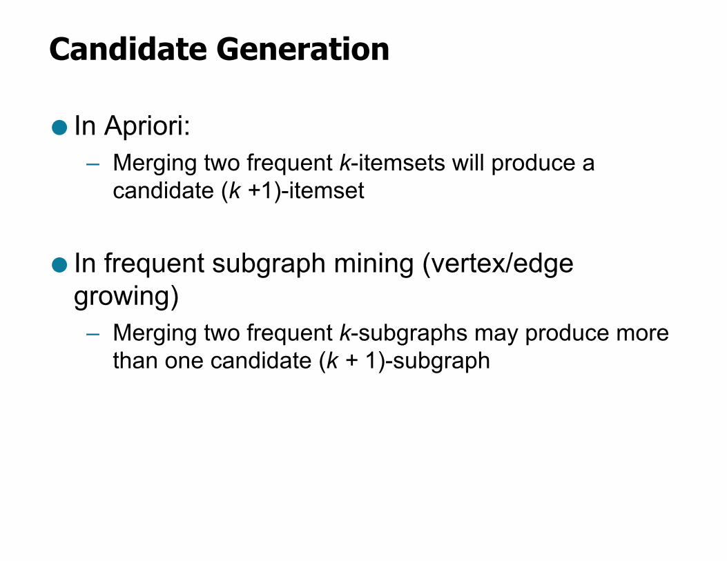
● In Apriori:– Merging two frequent k-itemsets will produce a
candidate (k +1)-itemset
● In frequent subgraph mining (vertex/edge growing)– Merging two frequent k-subgraphs may produce more
than one candidate (k + 1)-subgraph
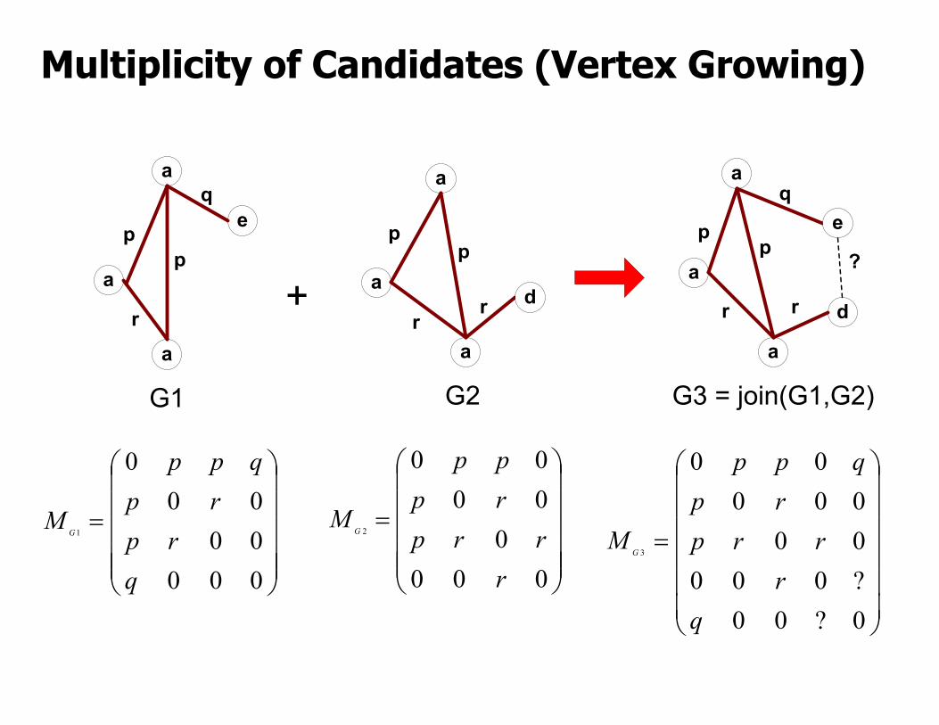
Multiplicity of Candidates (Vertex Growing)
a
a
e
a
p
q
r
p
a
a
a
p
rr
d
G1 G2
p
÷÷÷÷÷
ø
ö
ççççç
è
æ
=
0000000
0
1
qrp
rpqpp
MG
÷÷÷÷÷
ø
ö
ççççç
è
æ
=
00000000
2
rrrp
rppp
MG
a
a
a
p
q
r
ep
÷÷÷÷÷÷
ø
ö
çççççç
è
æ
=
0?00?00000000
00
3
qrrrp
rpqpp
MG
G3 = join(G1,G2)
dr
?
+
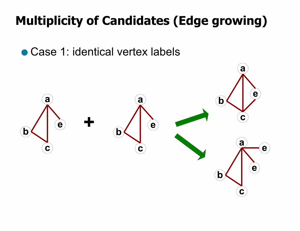
Multiplicity of Candidates (Edge growing)
● Case 1: identical vertex labels
a
be
c
a
be
c
+
a
be
c
ea
be
c
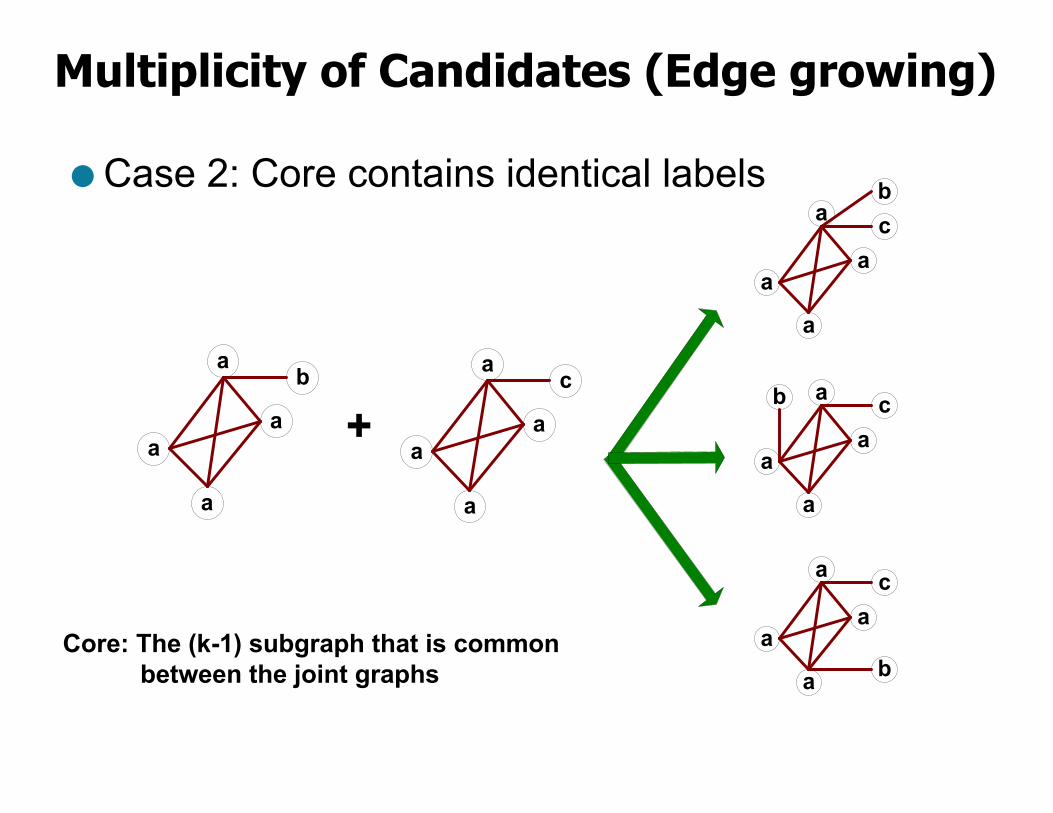
Multiplicity of Candidates (Edge growing)
● Case 2: Core contains identical labels
+
a
aa
a
cb
a
aa
a
c
a
aa
a
c
b
b
a
aa
a
b a
aa
a
c
Core: The (k-1) subgraph that is commonbetween the joint graphs
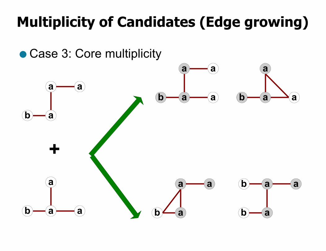
Multiplicity of Candidates (Edge growing)
● Case 3: Core multiplicity
a
ab
+
a
a
a ab
a ab
a
a
ab
a a
ab
ab
a ab
a a
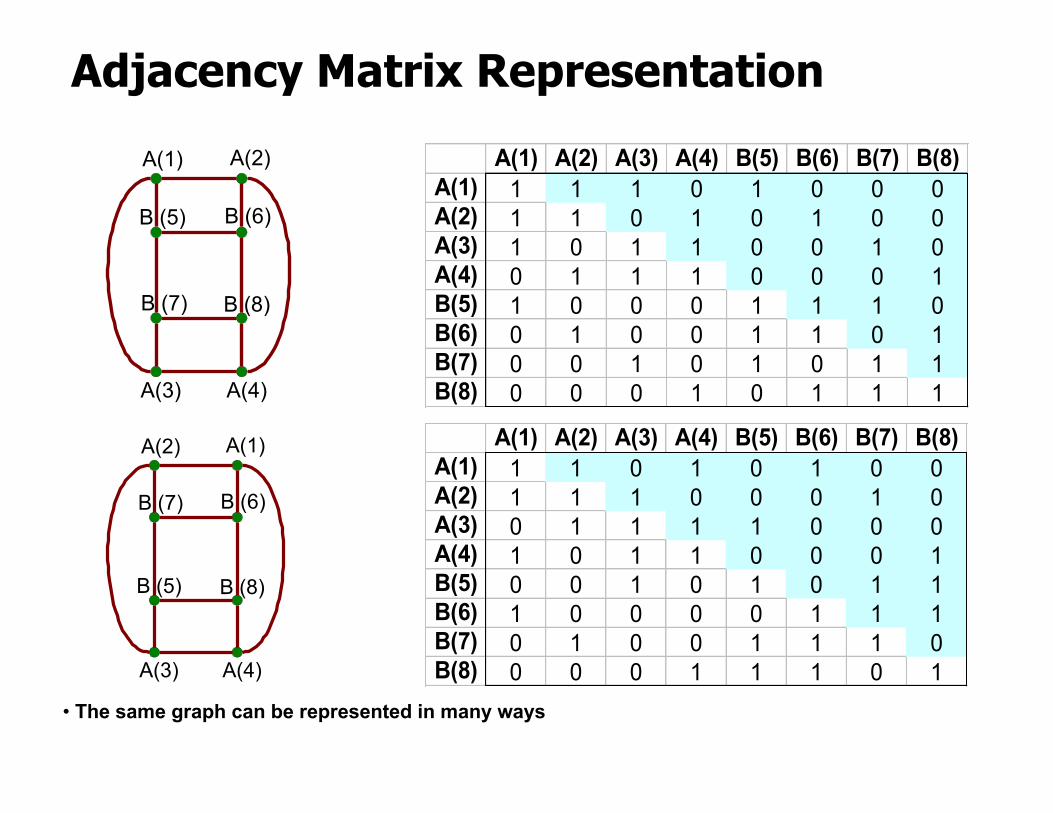
Adjacency Matrix RepresentationA(1) A(2)
B (6)
A(4)
B (5)
A(3)
B (7) B (8)
A(1) A(2) A(3) A(4) B(5) B(6) B(7) B(8)A(1) 1 1 1 0 1 0 0 0A(2) 1 1 0 1 0 1 0 0A(3) 1 0 1 1 0 0 1 0A(4) 0 1 1 1 0 0 0 1B(5) 1 0 0 0 1 1 1 0B(6) 0 1 0 0 1 1 0 1B(7) 0 0 1 0 1 0 1 1B(8) 0 0 0 1 0 1 1 1
A(2) A(1)
B (6)
A(4)
B (7)
A(3)
B (5) B (8)
A(1) A(2) A(3) A(4) B(5) B(6) B(7) B(8)A(1) 1 1 0 1 0 1 0 0A(2) 1 1 1 0 0 0 1 0A(3) 0 1 1 1 1 0 0 0A(4) 1 0 1 1 0 0 0 1B(5) 0 0 1 0 1 0 1 1B(6) 1 0 0 0 0 1 1 1B(7) 0 1 0 0 1 1 1 0B(8) 0 0 0 1 1 1 0 1
• The same graph can be represented in many ways
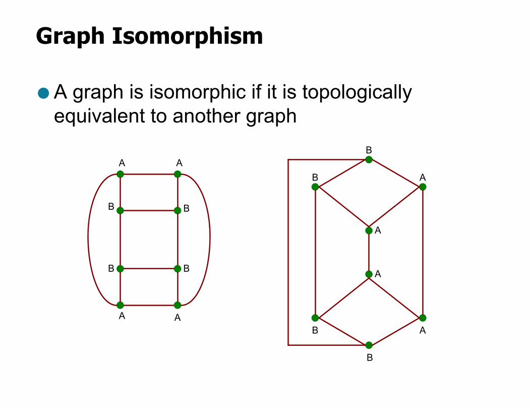
Graph Isomorphism
● A graph is isomorphic if it is topologically equivalent to another graph
A
A
A A
B A
B
A
B
B
A
A
B B
B
B
Graph Isomorphism
● Test for graph isomorphism is needed:– During candidate generation step, to determine
whether a candidate has been generated
– During candidate pruning step, to check whether its (k - 1)-subgraphs are frequent
– During candidate counting, to check whether a candidate is contained within another graph
Graph Isomorphism
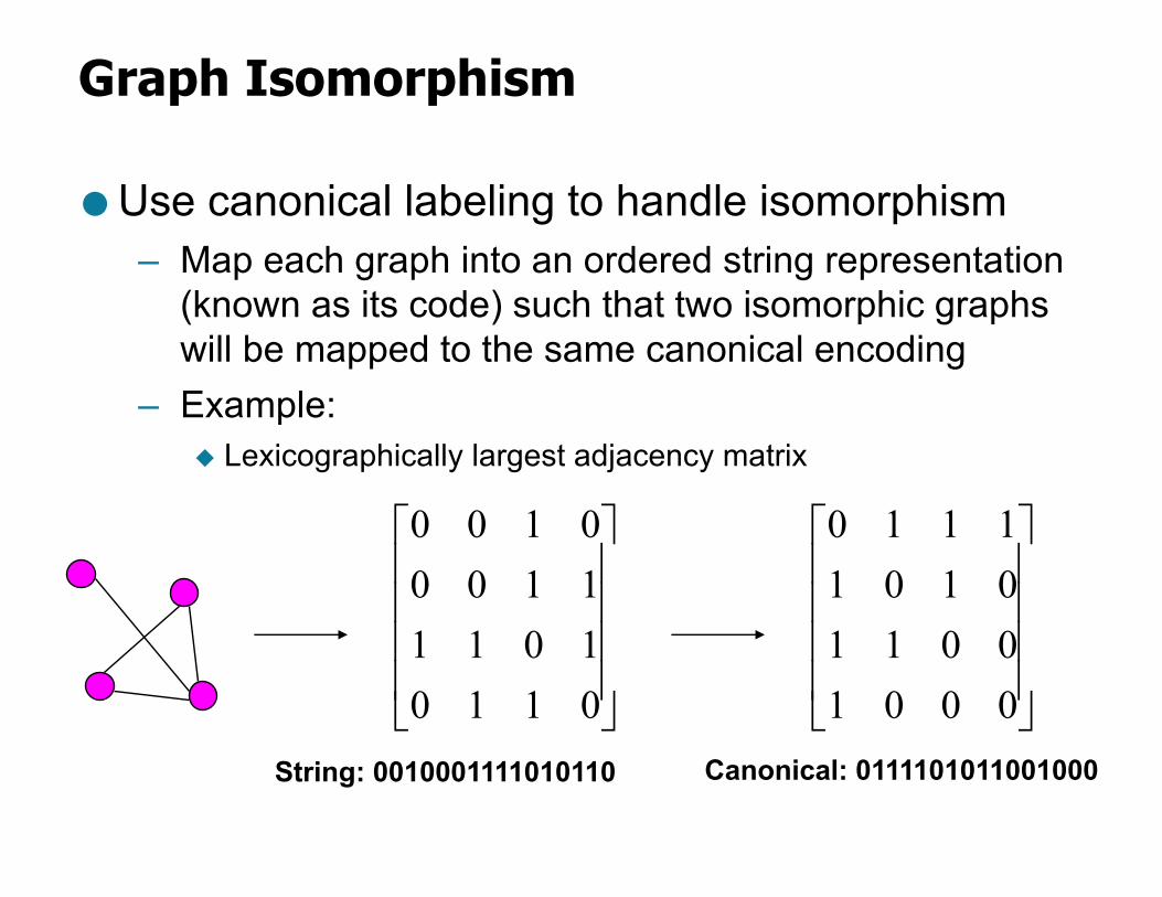
● Use canonical labeling to handle isomorphism– Map each graph into an ordered string representation
(known as its code) such that two isomorphic graphs will be mapped to the same canonical encoding
– Example: u Lexicographically largest adjacency matrix
úúúú
û
ù
êêêê
ë
é
0110101111000100
String: 0010001111010110
úúúú
û
ù
êêêê
ë
é
0001001101011110
Canonical: 0111101011001000