Embed Size (px)
Citation preview
Data Mining – Day 2
Fabiano Dalpiaz
Department of Information and
Communication Technology
University of Trento - Italy
http://www.dit.unitn.it/~dalpiaz
Database e Business Intelligence
A.A. 2007-2008
© P. Giorgini, F. Dalpiaz 2
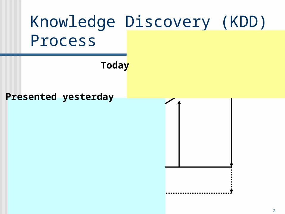
Knowledge Discovery (KDD) Process
Databases
Data Cleaning
Data Warehouse
Data Mining
Pattern Evaluation
Selection
Data Integration
Task-relevant Data
Presented yesterday
Today
© P. Giorgini, F. Dalpiaz 3
Outline
Data Mining techniques Frequent patterns, association rules
• Support and confidence
Classification and prediction• Decision trees• Bayesian classifiers• Support Vector Machines• Lazy learning
Cluster Analysis
Visualization of the results Summary
© P. Giorgini, F. Dalpiaz 4
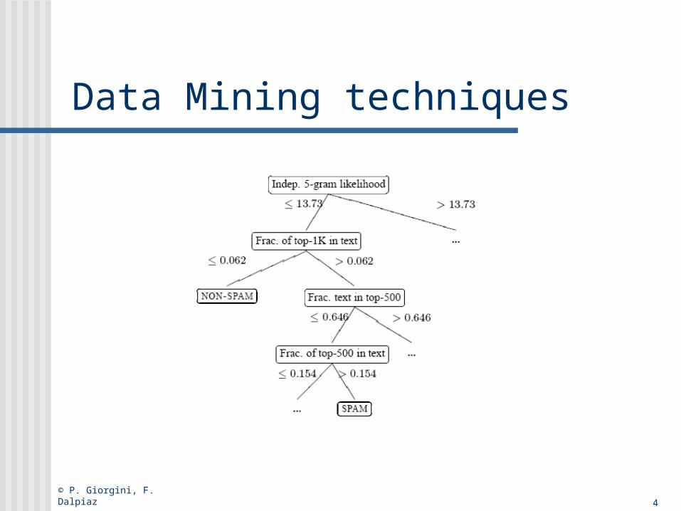
Data Mining techniques
© P. Giorgini, F. Dalpiaz 5
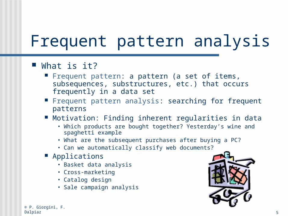
Frequent pattern analysis What is it?
Frequent pattern: a pattern (a set of items, subsequences, substructures, etc.) that occurs frequently in a data set
Frequent pattern analysis: searching for frequent patterns Motivation: Finding inherent regularities in data
• Which products are bought together? Yesterday’s wine and spaghetti example
• What are the subsequent purchases after buying a PC?• Can we automatically classify web documents?
Applications• Basket data analysis• Cross-marketing• Catalog design• Sale campaign analysis
© P. Giorgini, F. Dalpiaz 6
Basic Concepts: Frequent Patterns and Association Rules (1)
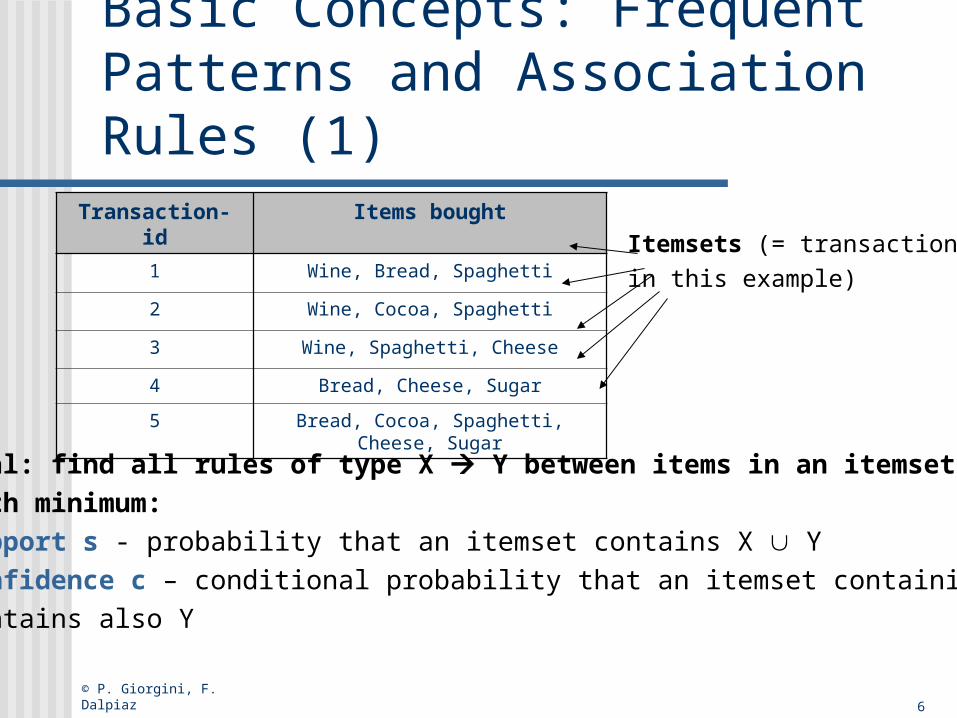
Transaction-id Items bought
1 Wine, Bread, Spaghetti
2 Wine, Cocoa, Spaghetti
3 Wine, Spaghetti, Cheese
4 Bread, Cheese, Sugar
5 Bread, Cocoa, Spaghetti, Cheese, Sugar
Itemsets (= transactionsin this example)
Goal: find all rules of type X Y between items in an itemsetwith minimum:Support s - probability that an itemset contains X YConfidence c – conditional probability that an itemset containing Xcontains also Y
© P. Giorgini, F. Dalpiaz 7
Basic Concepts: Frequent Patterns and Association Rules (2)
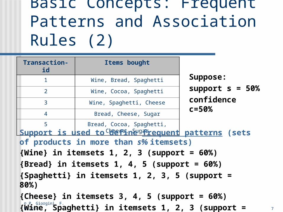
Transaction-id Items bought
1 Wine, Bread, Spaghetti
2 Wine, Cocoa, Spaghetti
3 Wine, Spaghetti, Cheese
4 Bread, Cheese, Sugar
5 Bread, Cocoa, Spaghetti, Cheese, Sugar
Suppose:support s = 50%confidence c=50%
Support is used to define frequent patterns (sets of products in more than s% itemsets){Wine} in itemsets 1, 2, 3 (support = 60%){Bread} in itemsets 1, 4, 5 (support = 60%){Spaghetti} in itemsets 1, 2, 3, 5 (support = 80%){Cheese} in itemsets 3, 4, 5 (support = 60%){Wine, Spaghetti} in itemsets 1, 2, 3 (support = 60%)
© P. Giorgini, F. Dalpiaz 8
Basic Concepts: Frequent Patterns and Association Rules (3)
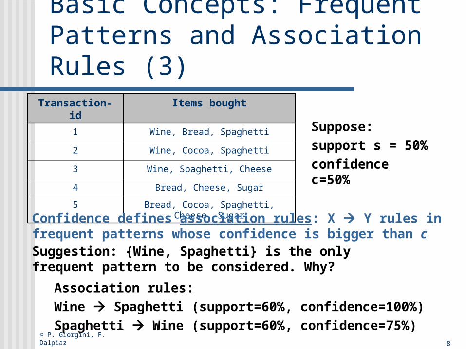
Transaction-id Items bought
1 Wine, Bread, Spaghetti
2 Wine, Cocoa, Spaghetti
3 Wine, Spaghetti, Cheese
4 Bread, Cheese, Sugar
5 Bread, Cocoa, Spaghetti, Cheese, Sugar
Suppose:support s = 50%confidence c=50%
Confidence defines association rules: X Y rules in frequent patterns whose confidence is bigger than cSuggestion: {Wine, Spaghetti} is the only frequent pattern to be considered. Why?
Association rules:Wine Spaghetti (support=60%, confidence=100%)Spaghetti Wine (support=60%, confidence=75%)
© P. Giorgini, F. Dalpiaz 9
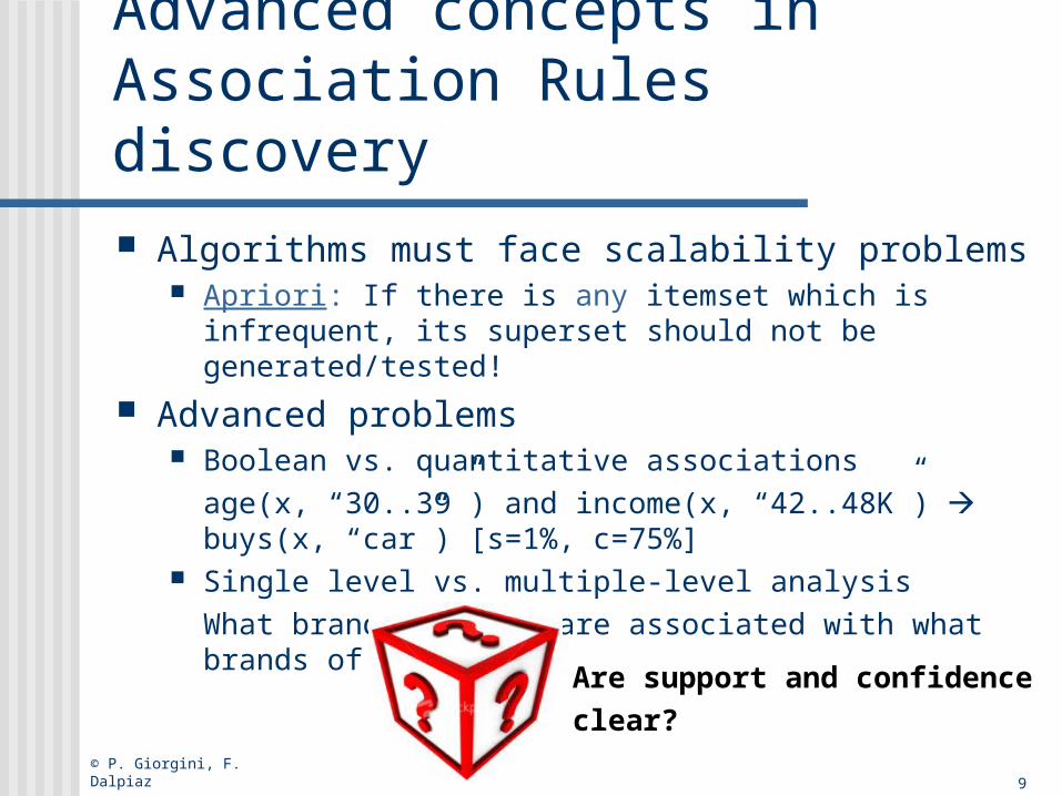
Advanced concepts in Association Rules discovery
Algorithms must face scalability problems Apriori: If there is any itemset which is infrequent, its superset
should not be generated/tested!
Advanced problems Boolean vs. quantitative associations
age(x, “30..39”) and income(x, “42..48K”) buys(x, “car”) [s=1%, c=75%]
Single level vs. multiple-level analysis
What brands of wine are associated with what brands of spaghetti?
Are support and confidenceclear?
© P. Giorgini, F. Dalpiaz 10
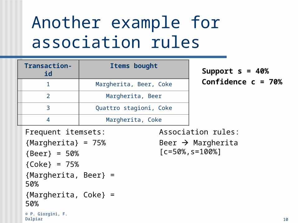
Another example for association rules
Transaction-id Items bought
1 Margherita, Beer, Coke
2 Margherita, Beer
3 Quattro stagioni, Coke
4 Margherita, Coke
Frequent itemsets:{Margherita} = 75%{Beer} = 50%{Coke} = 75%{Margherita, Beer} = 50%{Margherita, Coke} = 50%
Support s = 40%Confidence c = 70%
Association rules:Beer Margherita [c=50%,s=100%]
© P. Giorgini, F. Dalpiaz 11
Classification vs. Prediction
Classification Characterizes (describes) a set of items belonging to a training
set; these items are already classified according to a label attribute
The characterization is a model The model can be applied to classify new data (predict the class
they should belong to)
Prediction models continuous-valued functions, i.e., predicts unknown or
missing values
Applications Credit approval, target marketing, fraud detection
© P. Giorgini, F. Dalpiaz 12
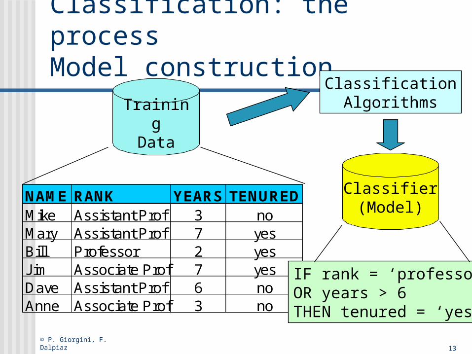
Classification: the process
1. Model construction The class label attribute defines the class each item should
belong to The set of items used for model construction is called training set The model is represented as classification rules, decision trees,
or mathematical formulae
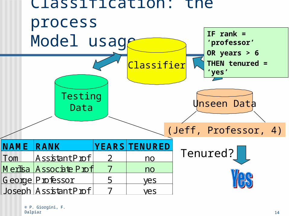
2. Model usage Estimate accuracy of the model
• On the training set
• On a generalization of the training set If the accuracy is acceptable, use the model to classify data
tuples whose class labels are not known
© P. Giorgini, F. Dalpiaz 13
Classification: the processModel construction
TrainingData
NAME RANK YEARS TENUREDMike Assistant Prof 3 noMary Assistant Prof 7 yesBill Professor 2 yesJim Associate Prof 7 yesDave Assistant Prof 6 noAnne Associate Prof 3 no
ClassificationAlgorithms
IF rank = ‘professor’OR years > 6THEN tenured = ‘yes’
Classifier(Model)
© P. Giorgini, F. Dalpiaz 14
Classification: the processModel usage
Classifier
TestingData
NAME RANK YEARS TENUREDTom Assistant Prof 2 noMerlisa Associate Prof 7 noGeorge Professor 5 yesJoseph Assistant Prof 7 yes
Unseen Data
(Jeff, Professor, 4)
Tenured?
IF rank = ‘professor’OR years > 6THEN tenured = ‘yes’
© P. Giorgini, F. Dalpiaz 15
Supervised vs. Unsupervised Learning
Supervised learning (classification) Supervision: The training data (observations, measurements,
etc.) are accompanied by labels indicating the class of the
observations
New data is classified based on the training set
Unsupervised learning (clustering) The class labels of training data is unknown
Given a set of measurements, observations, etc. with the aim of
establishing the existence of classes or clusters in the data
© P. Giorgini, F. Dalpiaz 16
Evaluating generated models Accuracy
classifier accuracy: predicting class label predictor accuracy: guessing value of predicted attributes
Speed time to construct the model (training time) time to use the model (classification/prediction time)
Robustness handling noise and missing values
Scalability efficiency in disk-resident databases
Interpretability understanding and insight provided by the model
© P. Giorgini, F. Dalpiaz 17
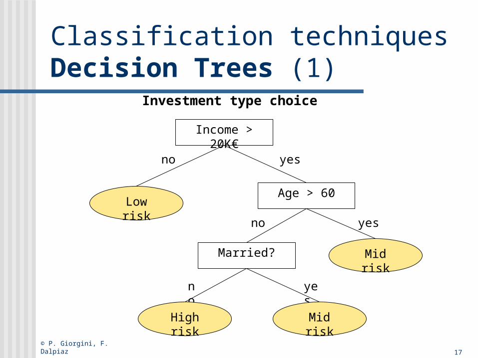
Classification techniquesDecision Trees (1)
Income > 20K€
Investment type choice
Age > 60
Married?
Low risk
no yes
no
Mid risk
yes
no
yes
High risk Mid risk
© P. Giorgini, F. Dalpiaz 18
Classification techniquesDecision Trees (2)
How are the attributes in decision trees selected? Two well-known indexes are used
• Information gain selects the most informative attribute in distinguishing the items between the classes
• It biases towards attributes with a large set of values
• Gain ratio faces the information gain limitations
© P. Giorgini, F. Dalpiaz 19
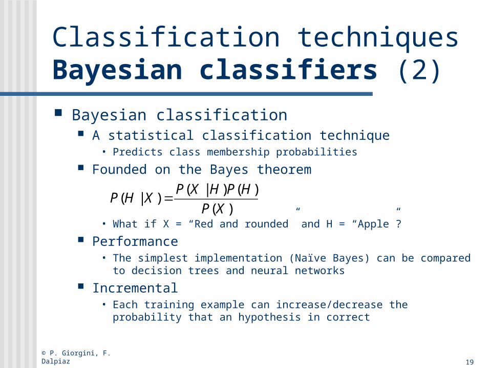
Classification techniquesBayesian classifiers (2)
Bayesian classification A statistical classification technique
• Predicts class membership probabilities
Founded on the Bayes theorem
• What if X = “Red and rounded” and H = “Apple”?
Performance• The simplest implementation (Naïve Bayes) can be compared to decision
trees and neural networks
Incremental• Each training example can increase/decrease the probability that an
hypothesis in correct
)(
)()|()|(
XP
HPHXPXHP
© P. Giorgini, F. Dalpiaz 20
5 minutes break!
© P. Giorgini, F. Dalpiaz 21
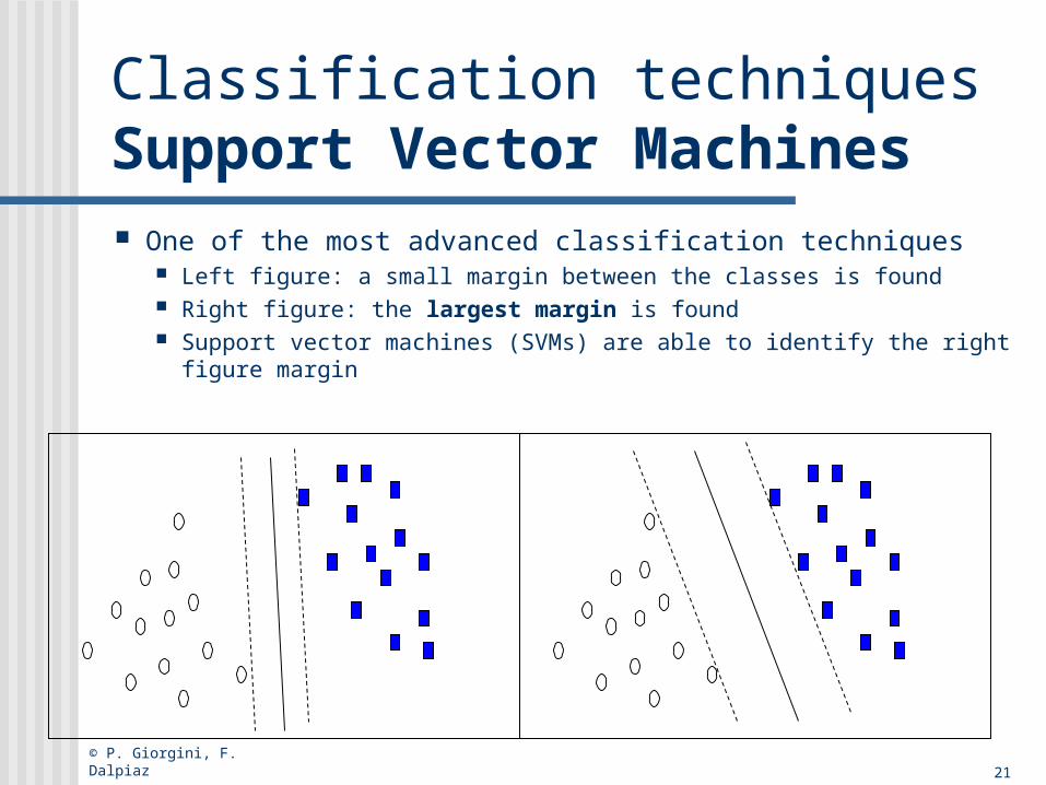
Classification techniquesSupport Vector Machines One of the most advanced classification techniques
Left figure: a small margin between the classes is found Right figure: the largest margin is found Support vector machines (SVMs) are able to identify the right figure margin
© P. Giorgini, F. Dalpiaz 22
Classification techniquesSVMs + Kernel Functions
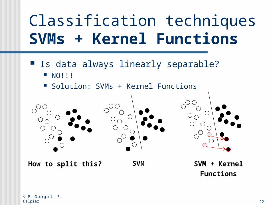
Is data always linearly separable? NO!!! Solution: SVMs + Kernel Functions
How to split this? SVM SVM + KernelFunctions
© P. Giorgini, F. Dalpiaz 23
Classification techniquesLazy learning
Lazy learning Simply stores training data (or only minor processing) and waits
until it is given a test tuple Less time in training but more time in predicting Uses a richer hypothesis space (many local linear functions),
and hence the accuracy is higher
Instance-based learning Subcategory of lazy learning Store training examples and delay the processing (“lazy
evaluation”) until a new instance must be classified An example: k-nearest neighbor approach
© P. Giorgini, F. Dalpiaz 24
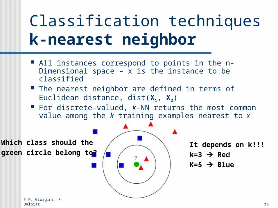
Classification techniquesk-nearest neighbor All instances correspond to points in the n-Dimensional
space – x is the instance to be classified The nearest neighbor are defined in terms of Euclidean
distance, dist(X1, X2) For discrete-valued, k-NN returns the most common value
among the k training examples nearest to x
It depends on k!!!k=3 RedK=5 Blue
Which class should thegreen circle belong to?
© P. Giorgini, F. Dalpiaz 25
Prediction techniquesAn overview Prediction is different from classification
Classification refers to predict categorical class label Prediction models continuous-valued functions
Major method for prediction: regression model the relationship between one or more independent or
predictor variables and a dependent or response variable
Regression analysis Linear and multiple regression Non-linear regression Other regression methods: generalized linear model, Poisson
regression, log-linear models, regression trees No details here
© P. Giorgini, F. Dalpiaz 26
What is cluster Analysis?
Cluster: a collection of data objects Similar to one another within the same cluster Dissimilar to the objects in other clusters
Cluster analysis Finding similarities between data according to the characteristics
found in the data and grouping similar data objects into clusters
It belongs to unsupervised learning Typical applications
As a stand-alone tool to get insight into data distribution As a preprocessing step for other algorithms (day 1 slides)
© P. Giorgini, F. Dalpiaz 27
Examples of cluster analysis
Marketing: Help marketers discover distinct groups in their customer bases
Land use: Identification of areas of similar land use in an earth observation
database
Insurance: Identifying groups of motor insurance policy holders with a high
average claim cost
City-planning: Identifying groups of houses according to their house type, value,
and geographical location
© P. Giorgini, F. Dalpiaz 28
Good clustering
A good clustering method will produce high quality clusters with high intra-class similarity low inter-class similarity
Dissimilarity/Similarity metric: Similarity is expressed in terms of a distance function, typically metric: d(i, j)
The definitions of distance functions are usually very different for interval-scaled, boolean, categorical, ordinal ratio, and vector variables.
It is hard to define “similar enough” or “good enough”
© P. Giorgini, F. Dalpiaz 29
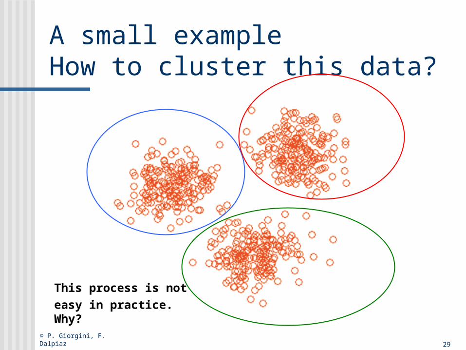
A small exampleHow to cluster this data?
This process is noteasy in practice. Why?
© P. Giorgini, F. Dalpiaz 30
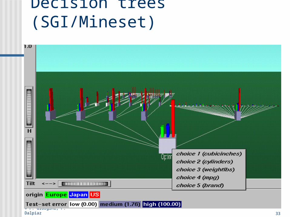
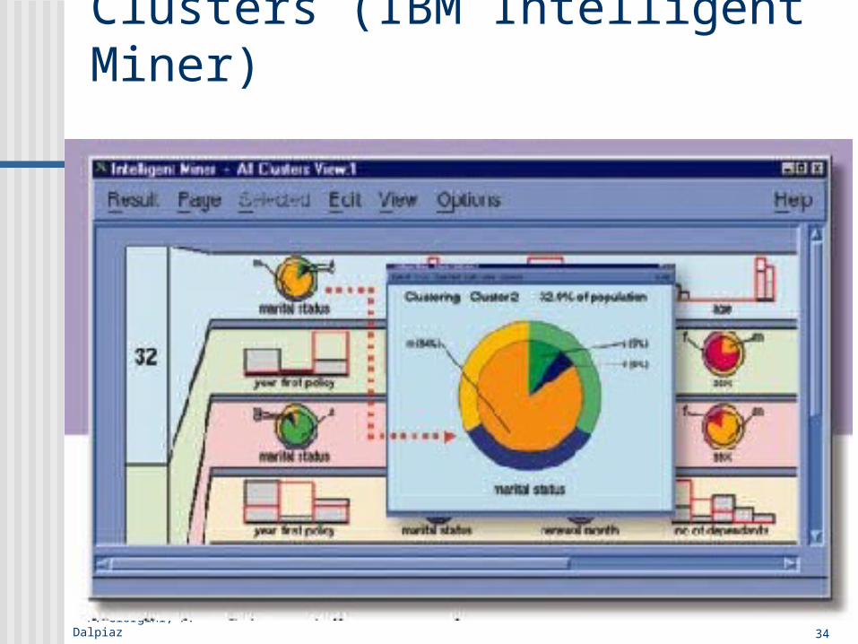
Visualization of the results
Presentation of the results or knowledge obtained from data mining in visual forms
Examples Scatter plots Association rules Decision trees Clusters
© P. Giorgini, F. Dalpiaz 31
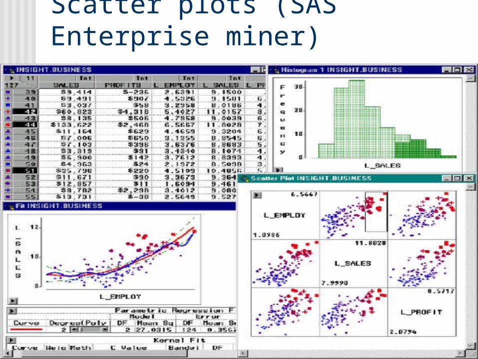
Scatter plots (SAS Enterprise miner)
© P. Giorgini, F. Dalpiaz 32
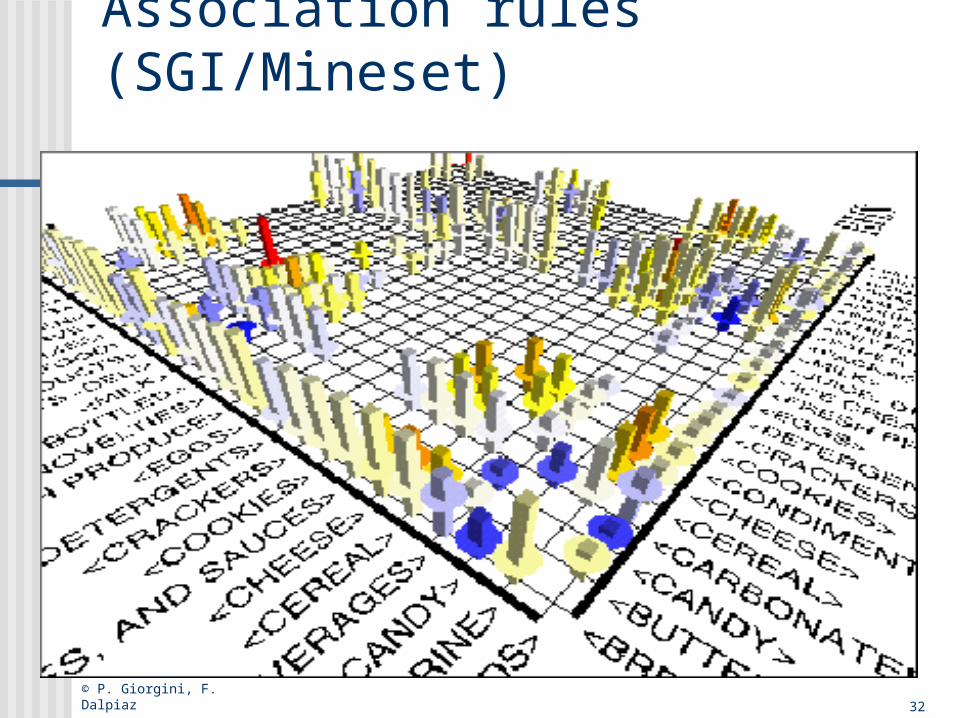
Association rules (SGI/Mineset)
© P. Giorgini, F. Dalpiaz 33
Decision trees (SGI/Mineset)
© P. Giorgini, F. Dalpiaz 34
Clusters (IBM Intelligent Miner)
© P. Giorgini, F. Dalpiaz 35
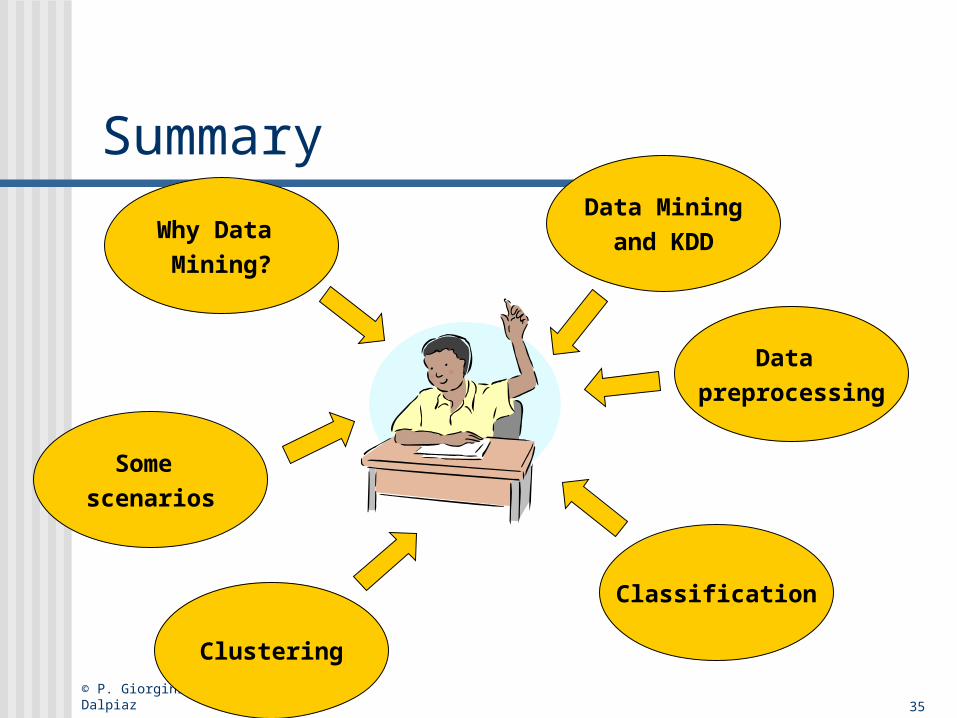
Summary
Why Data Mining?
Data Miningand KDD
Data preprocessing
Classification
Clustering
Some scenarios