Embed Size (px)
Citation preview

Data Mining: Introduction

Lots of data is being collected and warehoused
– Web data, e-commerce
– purchases at department/grocery stores
– Bank/Credit Card transactions
Computers have become cheaper and more powerful
Competitive Pressure is Strong
– Provide better, customized services for an edge (e.g. in Customer Relationship Management)
Why Mine Data? Commercial Viewpoint

Why Mine Data? Scientific Viewpoint
Data collected and stored at enormous speeds (GB/hour)
– remote sensors on a satellite
– telescopes scanning the skies
– microarrays generating gene expression data
– scientific simulations generating terabytes of data
Traditional techniques infeasible for raw data Data mining may help scientists
– in classifying and segmenting data
– in Hypothesis Formation

Mining Large Data Sets - Motivation
There is often information “hidden” in the data that is not readily evident
Human analysts may take weeks to discover useful information
Much of the data is never analyzed at all
The Data Gap
Number of analysts
From: R. Grossman, C. Kamath, V. Kumar, “Data Mining for Scientific and Engineering Applications”

What is Data Mining?
Many Definitions– Non-trivial extraction of implicit, previously
unknown and potentially useful information from data
– Exploration & analysis, by automatic or semi-automatic means, of large quantities of data in order to discover meaningful patterns

What is (not) Data Mining?
What is Data Mining?
– Certain names are more prevalent in certain US locations (O’Brien, O’Rurke, O’Reilly… in Boston area)
– Group together similar documents returned by search engine according to their context (e.g. Amazon rainforest, Amazon.com,)
What is not Data Mining?
– Look up phone number in phone directory
– Query a Web search engine for information about “Amazon”

Draws ideas from machine learning/AI, pattern recognition, statistics, and database systems
Traditional Techniquesmay be unsuitable due to
– Enormity of data
– High dimensionality of data
– Heterogeneous, distributed nature of data
Origins of Data Mining
Machine Learning/Pattern
Recognition
Statistics/AI
Data Mining
Database systems

Data Mining Tasks
Prediction Methods
– Use some variables to predict unknown or future values of other variables.
Description Methods
– Find human-interpretable patterns that describe the data.
From [Fayyad, et.al.] Advances in Knowledge Discovery and Data Mining, 1996

Data Mining Tasks...
Classification [Predictive]
Clustering [Descriptive]
Association Rule Discovery [Descriptive]
Sequential Pattern Discovery [Descriptive]
Regression [Predictive]
Deviation Detection [Predictive]

Classification

Classification: Definition
Given a collection of records (training set )– Each record contains a set of attributes, one of the
attributes is the class. Find a model for class attribute as a function
of the values of other attributes. Goal: previously unseen records should be
assigned a class as accurately as possible.– A test set is used to determine the accuracy of the
model. Usually, the given data set is divided into training and test sets, with training set used to build the model and test set used to validate it.

Classification Example
Tid Refund MaritalStatus
TaxableIncome Cheat
1 Yes Single 125K No
2 No Married 100K No
3 No Single 70K No
4 Yes Married 120K No
5 No Divorced 95K Yes
6 No Married 60K No
7 Yes Divorced 220K No
8 No Single 85K Yes
9 No Married 75K No
10 No Single 90K Yes10
categoric
al
categoric
al
continuous
class
Refund MaritalStatus
TaxableIncome Cheat
No Single 75K ?
Yes Married 50K ?
No Married 150K ?
Yes Divorced 90K ?
No Single 40K ?
No Married 80K ?10
TestSet
Training Set
ModelLearn
Classifier

Classification: Application 1
Direct Marketing
– Goal: Reduce cost of mailing by targeting a set of consumers likely to buy a new cell-phone product.
– Approach: Use the data for a similar product introduced before. We know which customers decided to buy and which
decided otherwise. This {buy, don’t buy} decision forms the class attribute.
Collect various demographic, lifestyle, and company-interaction related information about all such customers.
– Type of business, where they stay, how much they earn, etc. Use this information as input attributes to learn a classifier
model.

Classification: Application 2
Fraud Detection– Goal: Predict fraudulent cases in credit card
transactions.– Approach:
Use credit card transactions and the information on its account-holder as attributes.
– When does a customer buy, what does he buy, how often he pays on time, etc
Label past transactions as fraud or fair transactions. This forms the class attribute.
Learn a model for the class of the transactions. Use this model to detect fraud by observing credit card
transactions on an account.

Classification: Application 3
Customer Attrition/Churn:
– Goal: To predict whether a customer is likely to be lost to a competitor.
– Approach:Use detailed record of transactions with each of the
past and present customers, to find attributes.– How often the customer calls, where he calls, what time-of-the
day he calls most, his financial status, marital status, etc. Label the customers as loyal or disloyal.Find a model for loyalty.

Classification: Application 4
Sky Survey Cataloging
– Goal: To predict class (star or galaxy) of sky objects, especially visually faint ones, based on telescopic survey images.
– Thousands of images with 23,040 x 23,040 pixels per image.
– Approach: Segment the image. Measure image attributes (features) - 40 of them per object. Model the class based on these features. Success Story: found 16 new high red-shift quasars, some of
the farthest objects that are difficult to find!

Classifying Galaxies
Early
Intermediate
Late
Data Size: • 72 million stars, 20 million galaxies• Object Catalog: 9 GB• Image Database: 150 GB
Class: • Stages of
Formation
Attributes:• Image features, • Characteristics of
light waves received, etc.
Courtesy: http://aps.umn.edu

Clustering

Clustering Definition
Given a set of data points, each having a set of attributes, and a similarity measure among them, find clusters such that– Data points in one cluster are more similar to
one another.– Data points in separate clusters are less
similar to one another. Similarity Measures:
– Euclidean Distance if attributes are continuous.
– Other Problem-specific Measures.

Illustrating Clustering
Euclidean Distance Based Clustering in 3-D space.
Intracluster distancesare minimized
Intracluster distancesare minimized
Intercluster distancesare maximized
Intercluster distancesare maximized

Clustering: Application 1
Market Segmentation:– Goal: subdivide a market into distinct subsets of
customers where any subset may conceivably be selected as a market target to be reached with a distinct marketing mix.
– Approach: Collect different attributes of customers based on their
geographical and lifestyle related information. Find clusters of similar customers. Measure the clustering quality by observing buying patterns
of customers in same cluster vs. those from different clusters.

Clustering: Application 2
Document Clustering:
– Goal: To find groups of documents that are similar to each other based on the important terms appearing in them.
– Approach: To identify frequently occurring terms in each document. Form a similarity measure based on the frequencies of different terms. Use it to cluster.
– Gain: Information Retrieval can utilize the clusters to relate a new document or search term to clustered documents.

Illustrating Document Clustering
Clustering Points: 3204 Articles of Los Angeles Times. Similarity Measure: How many words are common in
these documents (after some word filtering).
Category TotalArticles
CorrectlyPlaced
Financial 555 364
Foreign 341 260
National 273 36
Metro 943 746
Sports 738 573
Entertainment 354 278

Clustering of S&P 500 Stock Data
Discovered Clusters Industry Group
1Applied-Matl-DOW N,Bay-Network-Down,3-COM-DOWN,
Cabletron-Sys-DOWN,CISCO-DOWN,HP-DOWN,DSC-Comm-DOW N,INTEL-DOWN,LSI-Logic-DOWN,
Micron-Tech-DOWN,Texas-Inst-Down,Tellabs-Inc-Down,Natl-Semiconduct-DOWN,Oracl-DOWN,SGI-DOW N,
Sun-DOW N
Technology1-DOWN
2Apple-Comp-DOW N,Autodesk-DOWN,DEC-DOWN,
ADV-Micro-Device-DOWN,Andrew-Corp-DOWN,Computer-Assoc-DOWN,Circuit-City-DOWN,
Compaq-DOWN, EMC-Corp-DOWN, Gen-Inst-DOWN,Motorola-DOW N,Microsoft-DOWN,Scientific-Atl-DOWN
Technology2-DOWN
3Fannie-Mae-DOWN,Fed-Home-Loan-DOW N,MBNA-Corp-DOWN,Morgan-Stanley-DOWN Financial-DOWN
4Baker-Hughes-UP,Dresser-Inds-UP,Halliburton-HLD-UP,
Louisiana-Land-UP,Phillips-Petro-UP,Unocal-UP,Schlumberger-UP
Oil-UP
Observe Stock Movements every day. Clustering points: Stock-{UP/DOWN} Similarity Measure: Two points are more similar if the
events described by them frequently happen together on the same day.
We used association rules to quantify a similarity measure.

Association Rule Discovery

Association Rule Discovery: Definition
Given a set of records each of which contain some number of items from a given collection;
– Produce dependency rules which will predict occurrence of an item based on occurrences of other items.
TID Items
1 Bread, Coke, Milk
2 Beer, Bread
3 Beer, Coke, Diaper, Milk
4 Beer, Bread, Diaper, Milk
5 Coke, Diaper, Milk
Rules Discovered: {Milk} --> {Coke} {Diaper, Milk} --> {Beer}
Rules Discovered: {Milk} --> {Coke} {Diaper, Milk} --> {Beer}

Association Rule Discovery: Application 1
Marketing and Sales Promotion:– Let the rule discovered be {Bagels, … } --> {Potato Chips}– Potato Chips as consequent => Can be used to
determine what should be done to boost its sales.– Bagels in the antecedent => Can be used to see
which products would be affected if the store discontinues selling bagels.
– Bagels in antecedent and Potato chips in consequent => Can be used to see what products should be sold with Bagels to promote sale of Potato chips!

Association Rule Discovery: Application 2
Supermarket shelf management.
– Goal: To identify items that are bought together by sufficiently many customers.
– Approach: Process the point-of-sale data collected with barcode scanners to find dependencies among items.
– A classic rule --If a customer buys potato chips, then he is very
likely to buy soda.So, don’t be surprised if you find chips and soda
next to each other

Association Rule Discovery: Application 3
Inventory Management:
– Goal: A consumer appliance repair company wants to anticipate the nature of repairs on its consumer products and keep the service vehicles equipped with right parts to reduce on number of visits to consumer households.
– Approach: Process the data on tools and parts required in previous repairs at different consumer locations and discover the co-occurrence patterns.

Sequential Pattern Discovery

Sequential Pattern Discovery: Definition
Given is a set of objects, with each object associated with its own timeline of events, find rules that predict strong sequential dependencies among different events.
Rules are formed by first disovering patterns. Event occurrences in the patterns are governed by timing constraints.
(A B) (C) (D E)
<= ms
<= xg >ng <= ws
(A B) (C) (D E)

Sequential Pattern Discovery: Examples
In telecommunications alarm logs,
– (Inverter_Problem Excessive_Line_Current)
(Rectifier_Alarm) --> (Fire_Alarm) In point-of-sale transaction sequences,
– Computer Bookstore:
(Intro_To_Visual_C) (C++_Primer) --> (Perl_for_dummies,Tcl_Tk)
– Athletic Apparel Store:
(Shoes) (Racket, Racketball) --> (Sports_Jacket)

Regression

Regression
Predict a value of a given continuous valued variable based on the values of other variables, assuming a linear or nonlinear model of dependency.
Greatly studied in statistics, neural network fields. Examples:
– Predicting sales amounts of new product based on advertising expenditure.
– Predicting wind velocities as a function of temperature, humidity, air pressure, etc.
– Time series prediction of stock market indices.

Regression
Independent variable (x)
Dep
en
den
t va
riab
le (
y)
The output of a regression is a function that predicts the dependent variable based upon values of the independent variables.
Simple regression fits a straight line to the data.
y’ = b0 + b1X ± є
b0 (y intercept)
B1 = slope= ∆y/ ∆x
є

Regression

Deviation/Anomaly Detection

Deviation/Anomaly Detection
Detect significant deviations from normal behavior Applications:
– Credit Card Fraud Detection
– Network Intrusion Detection
Typical network traffic at University level may reach over 100 million connections per day

Deviation/Anomaly Detection
N1 and N2 are regions of normal behavior
Points o1 and o2 are anomalies
Points in region O3 are anomalies
X
Y
N1
N2
o1
o2
O3

Challenges of Data Mining
Scalability Dimensionality Complex and Heterogeneous Data Data Quality Data Ownership and Distribution Privacy Preservation Streaming Data

What is Data?
Collection of data objects and their attributes
An attribute is a property or characteristic of an object
– Examples: eye color of a person, temperature, etc.
– Attribute is also known as variable, field, characteristic, or feature
A collection of attributes describe an object
– Object is also known as record, point, case, sample, entity, or instance
Tid Refund Marital Status
Taxable Income Cheat
1 Yes Single 125K No
2 No Married 100K No
3 No Single 70K No
4 Yes Married 120K No
5 No Divorced 95K Yes
6 No Married 60K No
7 Yes Divorced 220K No
8 No Single 85K Yes
9 No Married 75K No
10 No Single 90K Yes 10
Attributes
Objects

Attribute Values
Attribute values are numbers or symbols assigned to an attribute
Distinction between attributes and attribute values– Same attribute can be mapped to different
attribute values Example: height can be measured in feet or meters
– Different attributes can be mapped to the same set of values Example: Attribute values for ID and age are integers But properties of attribute values can be different
– ID has no limit but age has a maximum and minimum value

Types of Attributes
There are different types of attributes
– Nominal Examples: ID numbers, eye color, zip codes
– Ordinal Examples: rankings (e.g., taste of potato chips on a scale
from 1-10), grades, height in {tall, medium, short}
– Interval Examples: calendar dates, temperatures in Celsius or
Fahrenheit.
– Ratio Examples: temperature in Kelvin, length, time, counts

Properties of Attribute Values
The type of an attribute depends on which of the following properties it possesses:
– Distinctness: = – Order: < >
– Addition: + -
– Multiplication: * /
– Nominal attribute: distinctness
– Ordinal attribute: distinctness & order
– Interval attribute: distinctness, order & addition
– Ratio attribute: all 4 properties

Attribute Type
Description Examples Operations
Nominal The values of a nominal attribute are just different names, i.e., nominal attributes provide only enough information to distinguish one object from another. (=, )
zip codes, employee ID numbers, eye color, sex: {male, female}
mode, entropy, contingency correlation, 2 test
Ordinal The values of an ordinal attribute provide enough information to order objects. (<, >)
hardness of minerals, {good, better, best}, grades, street numbers
median, percentiles, rank correlation, run tests, sign tests
Interval For interval attributes, the differences between values are meaningful, i.e., a unit of measurement exists. (+, - )
calendar dates, temperature in Celsius or Fahrenheit
mean, standard deviation, Pearson's correlation, t and F tests
Ratio For ratio variables, both differences and ratios are meaningful. (*, /)
temperature in Kelvin, monetary quantities, counts, age, mass, length, electrical current
geometric mean, harmonic mean, percent variation

Attribute Level
Transformation Comments
Nominal Any permutation of values If all employee ID numbers were reassigned, would it make any difference?
Ordinal An order preserving change of values, i.e., new_value = f(old_value) where f is a monotonic function.
An attribute encompassing the notion of good, better best can be represented equally well by the values {1, 2, 3} or by { 0.5, 1, 10}.
Interval new_value =a * old_value + b where a and b are constants
Thus, the Fahrenheit and Celsius temperature scales differ in terms of where their zero value is and the size of a unit (degree).
Ratio new_value = a * old_value Length can be measured in meters or feet.

Discrete and Continuous Attributes
Discrete Attribute– Has only a finite or countably infinite set of values– Examples: zip codes, counts, or the set of words in a collection
of documents – Often represented as integer variables. – Note: binary attributes are a special case of discrete attributes
Continuous Attribute– Has real numbers as attribute values– Examples: temperature, height, or weight. – Practically, real values can only be measured and represented
using a finite number of digits.– Continuous attributes are typically represented as floating-point
variables.

Types of data sets
Record– Data Matrix
– Document Data
– Transaction Data
Graph– World Wide Web
– Molecular Structures
Ordered– Spatial Data
– Temporal Data
– Sequential Data
– Genetic Sequence Data
Unstructured Data

Important Characteristics of Structured Data
– Dimensionality Curse of Dimensionality
– Sparsity Only presence counts
– Resolution Patterns depend on the scale

Record Data
Data that consists of a collection of records, each of which consists of a fixed set of attributes
Tid Refund Marital Status
Taxable Income Cheat
1 Yes Single 125K No
2 No Married 100K No
3 No Single 70K No
4 Yes Married 120K No
5 No Divorced 95K Yes
6 No Married 60K No
7 Yes Divorced 220K No
8 No Single 85K Yes
9 No Married 75K No
10 No Single 90K Yes 10

Data Matrix
If data objects have the same fixed set of numeric attributes, then the data objects can be thought of as points in a multi-dimensional space, where each dimension represents a distinct attribute
Such data set can be represented by an m by n matrix, where there are m rows, one for each object, and n columns, one for each attribute
1.12.216.226.2512.65
1.22.715.225.2710.23
Thickness LoadDistanceProjection of y load
Projection of x Load
1.12.216.226.2512.65
1.22.715.225.2710.23
Thickness LoadDistanceProjection of y load
Projection of x Load

Document Data
Each document becomes a `term' vector,
– each term is a component (attribute) of the vector,
– the value of each component is the number of times the corresponding term occurs in the document.
Document 1
season
timeout
lost
win
game
score
ball
play
coach
team
Document 2
Document 3
3 0 5 0 2 6 0 2 0 2
0
0
7 0 2 1 0 0 3 0 0
1 0 0 1 2 2 0 3 0

Transaction Data
A special type of record data, where
– each record (transaction) involves a set of items.
– For example, consider a grocery store. The set of products purchased by a customer during one shopping trip constitute a transaction, while the individual products that were purchased are the items.
TID Items
1 Bread, Coke, Milk
2 Beer, Bread
3 Beer, Coke, Diaper, Milk
4 Beer, Bread, Diaper, Milk
5 Coke, Diaper, Milk

Graph Data
Examples: Generic graph and HTML Links
5
2
1
2
5
<a href="papers/papers.html#bbbb">Data Mining </a><li><a href="papers/papers.html#aaaa">Graph Partitioning </a><li><a href="papers/papers.html#aaaa">Parallel Solution of Sparse Linear System of Equations </a><li><a href="papers/papers.html#ffff">N-Body Computation and Dense Linear System Solvers

Chemical Data
Benzene Molecule: C6H6

Ordered Data
Sequences of transactions
An element of the sequence
Items/Events

Ordered Data
Genomic sequence data
GGTTCCGCCTTCAGCCCCGCGCCCGCAGGGCCCGCCCCGCGCCGTCGAGAAGGGCCCGCCTGGCGGGCGGGGGGAGGCGGGGCCGCCCGAGCCCAACCGAGTCCGACCAGGTGCCCCCTCTGCTCGGCCTAGACCTGAGCTCATTAGGCGGCAGCGGACAGGCCAAGTAGAACACGCGAAGCGCTGGGCTGCCTGCTGCGACCAGGG

Ordered Data
Spatio-Temporal Data
Average Monthly Temperature of land and ocean

Unstructured Data
No pre-defined data model or not organized in a pre-defined way
Typically text heavy In 1998 Merrill Lynch cited a rule of thumb that
somewhere between 80-90% of all potentiall usable business information may originate in unstructured form
Computer World states that unstructured information might account for more than 70%–80% of all data in organizations.

Unstructured Data
Unstructured Information Management Architecture (UIMA) is a component software architecture for analysis of unstructured information
– Developed by IBM
– Potential use: convert unstructured data into relational tables for traditional data analysis
Watson (Jeopardy Challenge) uses UIMA for real-time content analytics

Data Quality
What kinds of data quality problems? How can we detect problems with the data? What can we do about these problems?
Examples of data quality problems:
– Noise and outliers
– missing values
– duplicate data

Noise
Noise refers to modification of original values
– Examples: distortion of a person’s voice when talking on a poor phone and “snow” on television screen
Two Sine Waves Two Sine Waves + Noise

Outliers
Outliers are data objects with characteristics that are considerably different than most of the other data objects in the data set

Missing Values
Reasons for missing values– Information is not collected
(e.g., people decline to give their age and weight)– Attributes may not be applicable to all cases
(e.g., annual income is not applicable to children)
Handling missing values– Eliminate Data Objects– Estimate Missing Values– Ignore the Missing Value During Analysis– Replace with all possible values (weighted by their
probabilities)

Duplicate Data
Data set may include data objects that are duplicates, or almost duplicates of one another
– Major issue when merging data from heterogeous sources
Examples:
– Same person with multiple email addresses
Data cleaning
– Process of dealing with duplicate data issues

Data Preprocessing
Aggregation Sampling Dimensionality Reduction Feature subset selection Feature creation Discretization and Binarization Attribute Transformation

Aggregation
Combining two or more attributes (or objects) into a single attribute (or object)
Purpose
– Data reduction Reduce the number of attributes or objects
– Change of scale Cities aggregated into regions, states, countries, etc
– More “stable” data Aggregated data tends to have less variability

Aggregation
Standard Deviation of Average Monthly Precipitation
Standard Deviation of Average Yearly Precipitation
Variation of Precipitation in Australia

Sampling
Sampling is the main technique employed for data selection.– It is often used for both the preliminary investigation of the data
and the final data analysis.
Statisticians sample because obtaining the entire set of data of interest is too expensive or time consuming.
Sampling is used in data mining because processing the
entire set of data of interest is too expensive or time consuming.

Sampling …
The key principle for effective sampling is the following:
– using a sample will work almost as well as using the entire data sets, if the sample is representative
– A sample is representative if it has approximately the same property (of interest) as the original set of data

Types of Sampling
Simple Random Sampling– There is an equal probability of selecting any particular item
Sampling without replacement– As each item is selected, it is removed from the population
Sampling with replacement– Objects are not removed from the population as they are
selected for the sample. In sampling with replacement, the same object can be picked up more than once
Stratified sampling– Split the data into several partitions; then draw random samples
from each partition

Sample Size
8000 points 2000 Points 500 Points

Sample Size
What sample size is necessary to get at least one object from each of 10 groups.

Curse of Dimensionality
When dimensionality increases, data becomes increasingly sparse in the space that it occupies
Definitions of density and distance between points, which is critical for clustering and outlier detection, become less meaningful • Randomly generate 500 points
• Compute difference between max and min distance between any pair of points

Dimensionality Reduction
Purpose:– Avoid curse of dimensionality– Reduce amount of time and memory required
by data mining algorithms– Allow data to be more easily visualized– May help to eliminate irrelevant features or
reduce noise
Techniques– Principle Component Analysis– Singular Value Decomposition– Others: supervised and non-linear techniques

Dimensionality Reduction: PCA
Goal is to find a projection that captures the largest amount of variation in data
x2
x1
e

Dimensionality Reduction: PCA
Find the eigenvectors of the covariance matrix The eigenvectors define the new space
x2
x1
e

Example: Suppose we have the following sample of four observations made on three random variables X1, X2, and X3:
Find the three sample principal components y1, y2, and y3 based on the sample covariance matrix S:
X1 X2 X3
1.0 6.0 9.04.0 12.0 10.03.0 12.0 15.04.0 10.0 12.0

First we need the sample covariance matrix S:
and the corresponding eigenvalue-eigenvector pairs:
2.00 3.33 1.33
S = 3.33 8.00 4.67
1.33 4.67 7.00
ˆ ˆ
ˆ ˆ
ˆ ˆ
1 1
2 2
3 3
0.291000
λ = 13.21944,e = 0.734253
0.613345
0.415126
λ = 3.37916,e = 0.480690
-0.772403
0.861968
λ = 0.40140,e = -0.479385
0.164927

so the principal components are:
Note that
ˆ
ˆ
ˆ
'1 1 1 2 3
'2 2 1 2 3
'3 3 1 2 3
y = e x = 0.291000x + 0.734253x + 0.613345x
y = e x = 0.415126x + 0.480690x - 0.772403x
y = e x = 0.861968x - 0.479385x + 0.164927x
ˆ ˆ ˆ11 22 33
1 2 3
s + s + s = 2.0 + 8.0 + 7.0 = 17.0
= 13.21944 + 3.37916 + 0.40140 = λ + λ + λ

and the proportion of total population variance due to the each principal component is
Note that the third principal component is relatively irrelevant!
ˆ
ˆ1
p
ii=1
λ 13.21944= = 0.777613814
17.0λ
ˆ
ˆ2
p
ii=1
λ 3.37916= = 0.198774404
17.0λ
ˆ
ˆ3
p
ii=1
λ 0.40140= = 0.023611782
17.0λ

Feature Subset Selection
Another way to reduce dimensionality of data
Redundant features – duplicate much or all of the information
contained in one or more other attributes– Example: purchase price of a product and the
amount of sales tax paid
Irrelevant features– contain no information that is useful for the data
mining task at hand– Example: students' ID is often irrelevant to the
task of predicting students' GPA

Feature Subset Selection
Techniques:
– Brute-force approch:Try all possible feature subsets as input to data mining algorithm
– Embedded approaches: Feature selection occurs naturally as part of the data mining algorithm
– Filter approaches: Features are selected before data mining algorithm is run
– Wrapper approaches: Use the data mining algorithm as a black box to find best subset of attributes

Feature Creation
Create new attributes that can capture the important information in a data set much more efficiently than the original attributes
Three general methodologies:
– Feature Extraction domain-specific
– Mapping Data to New Space
– Feature Construction combining features

Mapping Data to a New Space
Two Sine Waves Two Sine Waves + Noise Frequency
Fourier transform Wavelet transform

Discretization Using Class Labels
Entropy based approach
3 categories for both x and y 5 categories for both x and y

Discretization Without Using Class Labels
Data Equal interval width
Equal frequency K-means

Attribute Transformation
A function that maps the entire set of values of a given attribute to a new set of replacement values such that each old value can be identified with one of the new values
– Simple functions: xk, log(x), ex, |x|
– Standardization and Normalization

Similarity and Dissimilarity
Similarity
– Numerical measure of how alike two data objects are.
– Is higher when objects are more alike.
– Often falls in the range [0,1] Dissimilarity
– Numerical measure of how different are two data objects
– Lower when objects are more alike
– Minimum dissimilarity is often 0
– Upper limit varies Proximity refers to a similarity or dissimilarity

Similarity/Dissimilarity for Simple Attributes
p and q are the attribute values for two data objects.
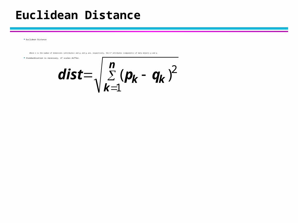
Euclidean Distance
Euclidean Distance
Where n is the number of dimensions (attributes) and pk and qk are, respectively, the kth attributes (components) of data objects p and q.
Standardization is necessary, if scales differ.
n
kkk qpdist
1
2)(

Euclidean Distance
0
1
2
3
0 1 2 3 4 5 6
p1
p2
p3 p4
point x yp1 0 2p2 2 0p3 3 1p4 5 1
Distance Matrix
p1 p2 p3 p4p1 0 2.828 3.162 5.099p2 2.828 0 1.414 3.162p3 3.162 1.414 0 2p4 5.099 3.162 2 0

Minkowski Distance
Minkowski Distance is a generalization of Euclidean Distance
Where r is a parameter, n is the number of dimensions (attributes) and pk and qk are, respectively, the kth attributes (components) or data objects p and q.
rn
k
rkk qpdist
1
1)||(

Minkowski Distance: Examples
r = 1. City block (Manhattan, taxicab, L1 norm) distance. – A common example of this is the Hamming distance, which is just the
number of bits that are different between two binary vectors
r = 2. Euclidean distance
r . “supremum” (Lmax norm, L norm) distance. – This is the maximum difference between any component of the vectors
Do not confuse r with n, i.e., all these distances are defined for all numbers of dimensions.

Minkowski Distance
Distance Matrix
point x yp1 0 2p2 2 0p3 3 1p4 5 1
L1 p1 p2 p3 p4p1 0 4 4 6p2 4 0 2 4p3 4 2 0 2p4 6 4 2 0
L2 p1 p2 p3 p4p1 0 2.828 3.162 5.099p2 2.828 0 1.414 3.162p3 3.162 1.414 0 2p4 5.099 3.162 2 0
L p1 p2 p3 p4
p1 0 2 3 5p2 2 0 1 3p3 3 1 0 2p4 5 3 2 0

Common Properties of a Distance
Distances, such as the Euclidean distance, have some well known properties.
1. d(p, q) 0 for all p and q and d(p, q) = 0 only if p = q. (Positive definiteness)
2. d(p, q) = d(q, p) for all p and q. (Symmetry)
3. d(p, r) d(p, q) + d(q, r) for all points p, q, and r. (Triangle Inequality)
where d(p, q) is the distance (dissimilarity) between points (data objects), p and q.
1. A distance that satisfies these properties is a metric

Common Properties of a Similarity
Similarities, also have some well known properties.
1. s(p, q) = 1 (or maximum similarity) only if p = q.
2. s(p, q) = s(q, p) for all p and q. (Symmetry)
where s(p, q) is the similarity between points (data objects), p and q.

Similarity Between Binary Vectors
Common situation is that objects, p and q, have only binary attributes
Compute similarities using the following quantitiesM01 = the number of attributes where p was 0 and q was 1
M10 = the number of attributes where p was 1 and q was 0
M00 = the number of attributes where p was 0 and q was 0
M11 = the number of attributes where p was 1 and q was 1
Simple Matching and Jaccard Coefficients SMC = number of matches / number of attributes
= (M11 + M00) / (M01 + M10 + M11 + M00)
J = number of 11 matches / number of not-both-zero attributes values
= (M11) / (M01 + M10 + M11)

SMC versus Jaccard: Example
p = 1 0 0 0 0 0 0 0 0 0
q = 0 0 0 0 0 0 1 0 0 1
M01 = 2 (the number of attributes where p was 0 and q was 1)
M10 = 1 (the number of attributes where p was 1 and q was 0)
M00 = 7 (the number of attributes where p was 0 and q was 0)
M11 = 0 (the number of attributes where p was 1 and q was 1)
SMC = (M11 + M00)/(M01 + M10 + M11 + M00) = (0+7) / (2+1+0+7) = 0.7
J = (M11) / (M01 + M10 + M11) = 0 / (2 + 1 + 0) = 0

Cosine Similarity
If d1 and d2 are two document vectors, then
cos( d1, d2 ) = (d1 d2) / ||d1|| ||d2|| ,
where indicates vector dot product and || d || is the length of vector d.
Example:
d1 = 3 2 0 5 0 0 0 2 0 0
d2 = 1 0 0 0 0 0 0 1 0 2
d1 d2= 3*1 + 2*0 + 0*0 + 5*0 + 0*0 + 0*0 + 0*0 + 2*1 + 0*0 + 0*2 = 5
||d1|| = (3*3+2*2+0*0+5*5+0*0+0*0+0*0+2*2+0*0+0*0)0.5 = (42) 0.5 = 6.481
||d2|| = (1*1+0*0+0*0+0*0+0*0+0*0+0*0+1*1+0*0+2*2) 0.5 = (6) 0.5 = 2.245
cos( d1, d2 ) = .3150

Correlation
Correlation measures the linear relationship between objects
To compute correlation, we standardize data objects, p and q, and then take their dot product
)(/))(( pstdpmeanpp kk
)(/))(( qstdqmeanqq kk
qpqpncorrelatio ),(

Visually Evaluating Correlation
Scatter plots showing the similarity from –1 to 1.