Embed Size (px)
Citation preview

DATA MINING
THE DATA MINING PIPELINEWhat is data?
The data mining pipeline: collection, preprocessing, mining, and post-processing
Sampling, feature extraction and normalization
Exploratory analysis of data – basic statistics

What is data mining again?
• “Data Mining is the study of collecting, processing, analyzing, and
gaining useful insights from data” – Charu Aggarwal
• Essentially, anything that has to do with data is data mining
Data Data Mining Value

What is Data Mining?
• Data mining is the use of efficient techniques for the analysis of very large collections of data and the extraction of useful and possibly unexpectedpatterns in data.
• “Data mining is the analysis of (often large) observational data sets to findunsuspected relationships and to summarize the data in novel ways that are both understandable and useful to the data analyst” (Hand, Mannila, Smyth)
• “Data mining is the discovery of models for data” (Rajaraman, Ullman)• We can have the following types of models
• Models that explain the data (e.g., a single function)
• Models that predict the future data instances.
• Models that summarize the data
• Models the extract the most prominent features of the data.

Why do we need data mining?
• Really huge amounts of complex data generated from multiple sources and interconnected in different ways• Scientific data from different disciplines
• Weather, astronomy, physics, biological microarrays, genomics
• Huge text collections• The Web, scientific articles, news, tweets, facebook postings.
• Transaction data• Retail store records, credit card records
• Behavioral data• Mobile phone data, query logs, browsing behavior, ad clicks
• Networked data• The Web, Social Networks, IM networks, email network, biological networks.
• All these types of data can be combined in many ways• Facebook has a network, text, images, user behavior, ad transactions.
• We need to analyze this data to extract knowledge• Knowledge can be used for commercial or scientific purposes.
• Our solutions should scale to the size of the data
• “Data is the new oil” – Clive Humby• Data Science: Use data to improve any process.

What is Data?
• Collection of data objects and their attributes
• An attribute is a property or characteristic of an object• Examples: name, date of birth, height, occupation.
• Attribute is also known as variable, field, characteristic, or feature
• For each object the attributes take some values.
• The collection of attribute-value pairsdescribes a specific object• Object is also known as record, point, case,
sample, entity, or instance
Tid Refund Marital Status
Taxable Income Cheat
1 Yes Single 125K No
2 No Married 100K No
3 No Single 70K No
4 Yes Married 120K No
5 No Divorced 95K Yes
6 No Married 60K No
7 Yes Divorced 220K No
8 No Single 85K Yes
9 No Married 75K No
10 No Single 90K Yes 10
Attributes
Objects
Size (n): Number of objects
Dimensionality (d): Number of attributes
Sparsity: Number of populated
object-attribute pairs

Relational data
• The term comes from DataBases, where we assume data is stored in a relational table with a fixed schema (fixed set of attributes)• In Databases, it is usually assumed that the
table is dense (few null values)
• There are a lot of data in this form• E.g., census data
• There are also a lot of data which do not fit well in this form• Sparse data: Many missing values
• Not easy to define a fixed schema
Tid Refund Marital Status
Taxable Income Cheat
1 Yes Single 125K No
2 No Married 100K No
3 No Single 70K No
4 Yes Married 120K No
5 No Divorced 95K NULL
6 No Married 60K No
7 Yes Divorced 220K No
8 No NULL 85K Yes
9 No Married 75K No
10 No Single 90K Yes 10
Attributes = Table columns
Objects =
Table rows
Example of a relational table

Types of Attributes
• There are different types of attributes
• Numeric
• Examples: dates, temperature, time, length, value, count.
• Discrete (counts) vs Continuous (temperature)
• Special case: Binary/Boolean attributes (yes/no, exists/not exists)
• Categorical
• Examples: eye color, zip codes, strings, rankings (e.g, good, fair, bad),
height in {tall, medium, short}
• Nominal (no order or comparison) vs Ordinal (order but not comparable)

Numeric Relational Data
• If data objects have the same fixed set of numeric attributes, then the data
objects can be thought of as points/vectors in a multi-dimensional space, where
each dimension represents a distinct attribute
• Such data set can be represented by an n-by-d data matrix, where there are n
rows, one for each object, and d columns, one for each attribute
Temperature Humidity Pressure
O1 30 0.8 90
O2 32 0.5 80
O3 24 0.3 95
30 0.8 90
32 0.5 80
24 0.3 95
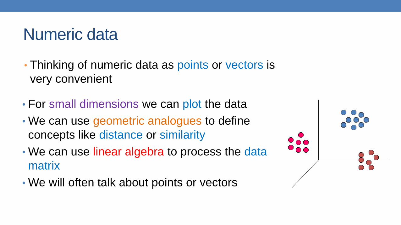
Numeric data
• For small dimensions we can plot the data
• We can use geometric analogues to define
concepts like distance or similarity
• We can use linear algebra to process the data
matrix
• We will often talk about points or vectors
• Thinking of numeric data as points or vectors is
very convenient

Categorical Relational Data
• Data that consists of a collection of records, each of which consists
of a fixed set of categorical attributes
ID Number Zip Code Marital
Status
Income
Bracket
1129842 45221 Single High
2342345 45223 Married Low
1234542 45221 Divorced High
1243535 45224 Single Medium

Mixed Relational Data
• Data that consists of a collection of records, each of which consists
of a fixed set of both numeric and categorical attributes
ID
Number
Zip Code Age Marital
Status
Income Income
Bracket
1129842 45221 55 Single 250000 High
2342345 45223 25 Married 30000 Low
1234542 45221 45 Divorced 200000 High
1243535 45224 43 Single 150000 Medium

Mixed Relational Data
• Data that consists of a collection of records, each of which consists
of a fixed set of both numeric and categorical attributes
ID
Number
Zip
Code
Age Marital
Status
Income Income
Bracket
Refund
1129842 45221 55 Single 250000 High No
2342345 45223 25 Married 30000 Low Yes
1234542 45221 45 Divorced 200000 High No
1243535 45224 43 Single 150000 Medium No
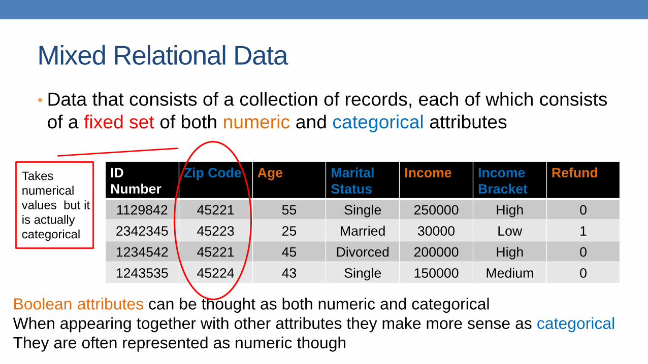
Mixed Relational Data
• Data that consists of a collection of records, each of which consists
of a fixed set of both numeric and categorical attributes
ID
Number
Zip Code Age Marital
Status
Income Income
Bracket
Refund
1129842 45221 55 Single 250000 High 0
2342345 45223 25 Married 30000 Low 1
1234542 45221 45 Divorced 200000 High 0
1243535 45224 43 Single 150000 Medium 0
Boolean attributes can be thought as both numeric and categorical
When appearing together with other attributes they make more sense as categorical
They are often represented as numeric though
Takes
numerical
values but it
is actually
categorical
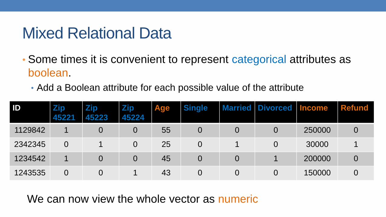
Mixed Relational Data
• Some times it is convenient to represent categorical attributes as
boolean.
• Add a Boolean attribute for each possible value of the attribute
ID Zip
45221
Zip
45223
Zip
45224
Age Single Married Divorced Income Refund
1129842 1 0 0 55 0 0 0 250000 0
2342345 0 1 0 25 0 1 0 30000 1
1234542 1 0 0 45 0 0 1 200000 0
1243535 0 0 1 43 0 0 0 150000 0
We can now view the whole vector as numeric

Mixed Relational Data
• Some times it is convenient to represent numerical attributes as
categorical.
• Group the values of the numerical attributes into bins
ID
Number
Zip Code Age Marital
Status
Income Income
Bracket
Refund
1129842 45221 50s Single High High 0
2342345 45223 20s Married Low Low 1
1234542 45221 40s Divorced High High 0
1243535 45224 40s Single Medium Medium 0

Binning
• Idea: split the range of the domain of the numerical attribute into
bins (intervals).
• Every bucket defines a categorical value
• How do we decide the number of bins?
• Depends on the granularity of the data that we want
200,00050,000
Low Medium High

Bucketization
• How do we decide the size of the bucket?• Depends on the data and our application
• Equi-width bins: All bins have the same size• Example: split time into decades
• Problem: some bins may be very sparse or empty
• Equi-size (depth) bins: Select the bins so that they all contain the same number of elements• This splits data into quantiles: top-10%, second 10% etc
• Some bins may be very small
• Equi-log bins:log 𝑒𝑛𝑑 − log 𝑠𝑡𝑎𝑟𝑡 is constant• The size of the previous bin is a fraction of the current one
• Better for skewed distributions
• Optimized bins: Use a 1-dimensional clustering algorithm to create the bins

Example
Blue: Equi-width [20,40,60,80]
Red: Equi-depth (2 points per bin)
Green: Equi-log (𝑒𝑛𝑑
𝑠𝑡𝑎𝑟𝑡= 2)

Physical data storage
• Stored in a Relational Database• Assumes a strict schema and relatively dense data (few missing/Null values)
• Tab or Comma separated files (TSV/CSV), Excel sheets, relational tables• Assumes a strict schema and relatively dense data (few missing/Null values)
• Flat file with triplets (record id, attribute, attribute value)• A very flexible data format, allows multiple values for the same attribute
(e.g., phone number)
• JSON, XML format• Standards for data description that are more flexible than relational tables
• There exist parsers for reading such data.

Examples
Comma Separated File
• Can be processed with simple
parsers, or loaded to excel or a
database
Triple-store
• Easy to deal with missing values
id,Name,Surname,Age,Zip
1,John,Smith,25,10021
2,Mary,Jones,50,96107
3,Joe ,Doe,80,80235
1, Name, John
1, Surname, Smith
1, Age, 25
1, Zip, 10021
2, Name, Mary
2, Surname, Jones
2, Age, 50
2, Zip, 96107
3, Name, Joe
3, Surname, Doe
3, Age, 80
3, Zip, 80235

ExamplesJSON EXAMPLE – Record of a person
{
"firstName": "John",
"lastName": "Smith",
"isAlive": true,
"age": 25,
"address": {
"streetAddress": "21 2nd Street",
"city": "New York",
"state": "NY",
"postalCode": "10021-3100"
},
"phoneNumbers": [
{
"type": "home",
"number": "212 555-1234"
},
{
"type": "office",
"number": "646 555-4567"
}
],
"children": [],
"spouse": null
}
XML EXAMPLE – Record of a person
<person>
<firstName>John</firstName>
<lastName>Smith</lastName>
<age>25</age>
<address>
<streetAddress>21 2nd Street</streetAddress>
<city>New York</city>
<state>NY</state>
<postalCode>10021</postalCode>
</address>
<phoneNumbers>
<phoneNumber>
<type>home</type>
<number>212 555-1234</number>
</phoneNumber>
<phoneNumber>
<type>fax</type>
<number>646 555-4567</number>
</phoneNumber>
</phoneNumbers>
<gender>
<type>male</type>
</gender>
</person>

Beyond relational data: Set data
• Each record is a set of items from a space of possible items
• Example: Transaction data
• Also called market-basket data
TID Items
1 Bread, Coke, Milk
2 Beer, Bread
3 Beer, Coke, Diaper, Milk
4 Beer, Bread, Diaper, Milk
5 Coke, Diaper, Milk

Set data
• Each record is a set of items from a space of possible items
• Example: Document data
• Also called bag-of-words representation
Doc Id Words
1 the, dog, followed, the, cat
2 the, cat, chased, the, cat
3 the, man, walked, the, dog

Vector representation of market-basket data
• Market-basket data can be represented, or thought of, as numeric
vector data
• The vector is defined over the set of all possible items
• The values are binary (the item appears or not in the set)
TID Items
1 Bread, Coke, Milk
2 Beer, Bread
3 Beer, Coke, Diaper, Milk
4 Beer, Bread, Diaper, Milk
5 Coke, Diaper, Milk
TID Bre
ad
Co
ke
Mil
k
Beer
Dia
per
1 1 1 1 0 0
2 1 0 0 1 0
3 0 1 1 1 1
4 1 0 1 1 1
5 0 1 1 0 1
Sparsity: Most entries are zero. Most baskets contain few items

Vector representation of document data
• Document data can be represented, or thought of, as numeric vector
data
• The vector is defined over the set of all possible words
• The values are the counts (number of times a word appears in the document)
Doc
Id the
do
g
foll
ow
s
cat
ch
ases
man
walk
s
1 2 1 1 1 0 0 0
2 2 0 0 2 1 0 0
3 1 1 0 0 0 1 1
Doc Id Words
1 the, dog, follows, the, cat
2 the, cat, chases, the, cat
3 the, man, walks, the, dog
Sparsity: Most entries are zero. Most documents contain few of the words

Physical data storage
• Usually set data is stored in flat files
• One line per set
• I heard so many good things about this place so I was pretty juiced to try it. I'm
from Cali and I heard Shake Shack is comparable to IN-N-OUT and I gotta say, Shake
Shake wins hands down. Surprisingly, the line was short and we waited about 10
MIN. to order. I ordered a regular cheeseburger, fries and a black/white shake. So
yummerz. I love the location too! It's in the middle of the city and the view is
breathtaking. Definitely one of my favorite places to eat in NYC.
• I'm from California and I must say, Shake Shack is better than IN-N-OUT, all day,
err'day.
0 1 2 3 4 5 6 7 8 9 10 11 12 13 14 15 16 17 18 19 20 21 22 23 24 25 26 27 28 29
30 31 32
33 34 35
36 37 38 39 40 41 42 43 44 45 46
38 39 47 48
38 39 48 49 50 51 52 53 54 55 56 57 58
32 41 59 60 61 62
3 39 48

Dependent data
• In tables we usually consider each object independent of each
other.
• In some cases, there are explicit dependencies between the data
• Ordered/Temporal data: We know the time order of the data
• Spatial data: Data that is placed on specific locations
• Spatiotemporal data: data with location and time
• Networked/Graph data: data with pairwise relationships between entities

Ordered Data
• Genomic sequence data
• Data is a long ordered string
GGTTCCGCCTTCAGCCCCGCGCC
CGCAGGGCCCGCCCCGCGCCGTC
GAGAAGGGCCCGCCTGGCGGGCG
GGGGGAGGCGGGGCCGCCCGAGC
CCAACCGAGTCCGACCAGGTGCC
CCCTCTGCTCGGCCTAGACCTGA
GCTCATTAGGCGGCAGCGGACAG
GCCAAGTAGAACACGCGAAGCGC
TGGGCTGCCTGCTGCGACCAGGG

Ordered Data
• Time series
• Sequence of ordered (over “time”) numeric values.

Ordered Data
• Sequence data: Similar to the time series but in this case we have
categorical values rather than numerical ones.
• Example: Event logs
fcrawler.looksmart.com - - [26/Apr/2000:00:00:12 -0400] "GET /contacts.html HTTP/1.0" 200 4595 "-" "FAST-WebCrawler/2.1
fcrawler.looksmart.com - - [26/Apr/2000:00:17:19 -0400] "GET /news/news.html HTTP/1.0" 200 16716 "-" "FAST-WebCrawler/2.1
ppp931.on.bellglobal.com - - [26/Apr/2000:00:16:12 -0400] "GET /download/windows/asctab31.zip HTTP/1.0" 200 1540096 "
123.123.123.123 - - [26/Apr/2000:00:23:48 -0400] "GET /pics/wpaper.gif HTTP/1.0" 200 6248 "http://www.jafsoft.com/asctortf/
123.123.123.123 - - [26/Apr/2000:00:23:47 -0400] "GET /asctortf/ HTTP/1.0" 200 8130 "http://search.netscape.com/Computers/
123.123.123.123 - - [26/Apr/2000:00:23:48 -0400] "GET /pics/5star2000.gif HTTP/1.0" 200 4005 "http://www.jafsoft.com/asctortf/
123.123.123.123 - - [26/Apr/2000:00:23:50 -0400] "GET /pics/5star.gif HTTP/1.0" 200 1031 "http://www.jafsoft.com/asctortf/
123.123.123.123 - - [26/Apr/2000:00:23:51 -0400] "GET /pics/a2hlogo.jpg HTTP/1.0" 200 4282 "http://www.jafsoft.com/asctortf/
123.123.123.123 - - [26/Apr/2000:00:23:51 -0400] "GET /cgi-bin/newcount?jafsof3&width=4&font=digital&noshow HTTP/1.0" 200 36 "

Spatial data
• Attribute values that can be arranged with geographic co-ordinates
• Measurements of temperature/pressure in different locations.
• Sales numbers in different stores
• The majority party in the country states (categorical)
• Such data can be nicely visualized.

Spatiotemporal data
• Data that have both spatial and temporal aspects
• Measurements in different locations over time
• Pressure, Temperature, Humidity
• Measurements that move in space over time
• Traffic, Trajectories of moving objects

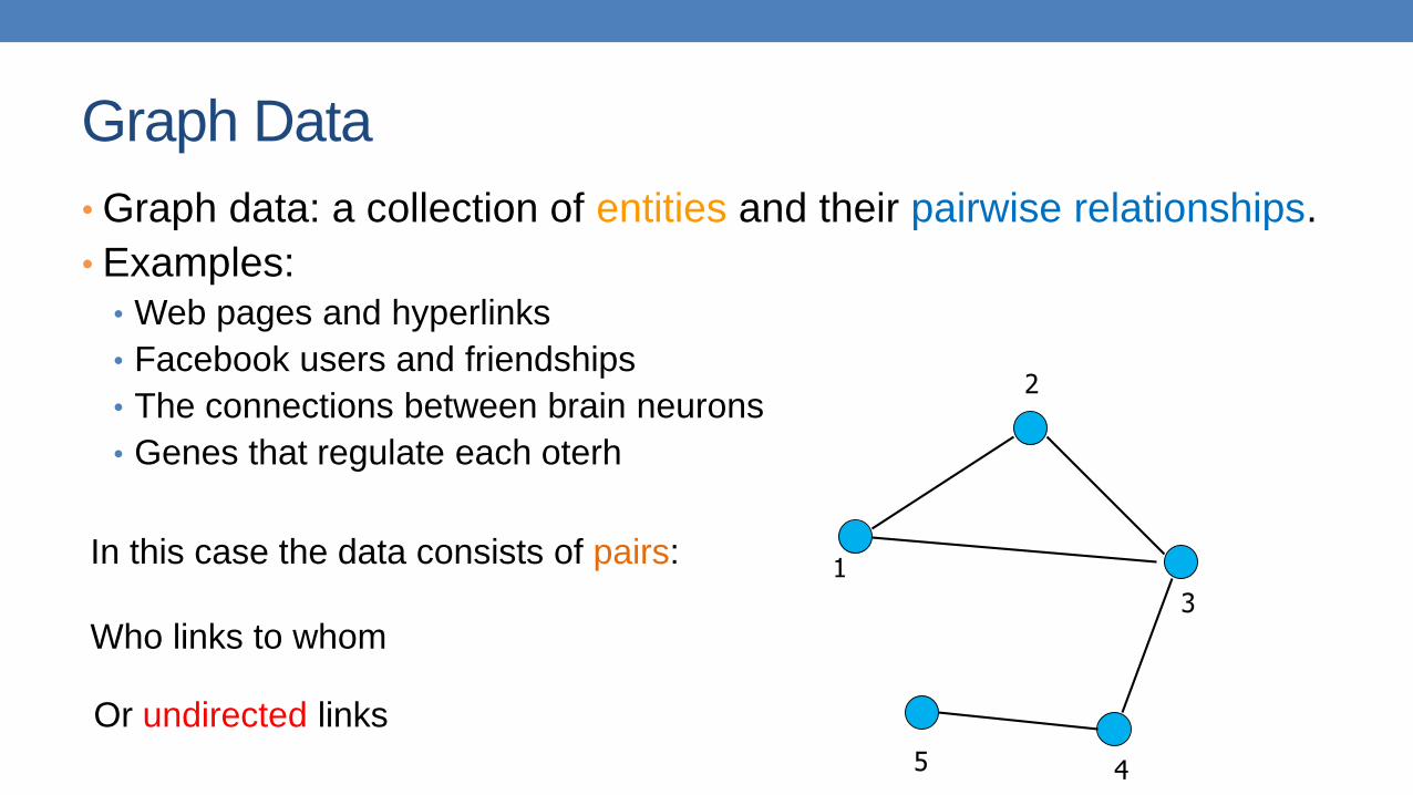
Graph Data
• Graph data: a collection of entities and their pairwise relationships.
• Examples:• Web pages and hyperlinks
• Facebook users and friendships
• The connections between brain neurons
• Genes that regulate each oterh
In this case the data consists of pairs:
Who links to whom
1
2
3
45We may have directed links
Graph Data
• Graph data: a collection of entities and their pairwise relationships.
• Examples:• Web pages and hyperlinks
• Facebook users and friendships
• The connections between brain neurons
• Genes that regulate each oterh
In this case the data consists of pairs:
Who links to whom
1
2
3
45
Or undirected links

Representation
• Adjacency matrix
• Very sparse, very wasteful, but useful conceptually
1
2
3
45
=
00000
10000
01010
00001
00110
A

Representation
• Adjacency list
• Not so easy to maintain
1
2
3
45
1: [2, 3]
2: [1, 3]
3: [1, 2, 4]
4: [3, 5]
5: [4]

Representation
• List of pairs
• The simplest and most efficient representation
1
2
3
45
(1,2)
(2,3)
(1,3)
(3,4)
(4,5)

Types of data: summary
• Numeric data: Each object is a point in a multidimensional space
• Categorical data: Each object is a vector of categorical values
• Set data: Each object is a set of values (with or without counts)
• Sets can also be represented as binary vectors, or vectors of counts
• Dependent data:
• Ordered sequences: Each object is an ordered sequence of values.
• Spatial data: objects are fixed on specific geographic locations
• Graph data: A collection of pairwise relationships

The data analysis pipeline
Data
PreprocessingData Mining
Result
Post-processing
Data
Collection
Mining is not the only step in the analysis process
The data mining part is about the analytical methods and algorithms for
extracting useful knowledge from the data.

The data analysis pipeline
• Today there is an abundance of data online (Twitter, Wikipedia, Web, Open data initiatives, etc)
• Collecting the data is a separate task• Customized crawlers, use of public APIs. Respect of crawling etiquette
• Which data should we collect?• We cannot necessarily collect everything so we need to make some choices before starting.
• How should we store them?
• In many cases when collecting data we also need to label them• E.g., how do we identify fraudulent transactions?
• E.g., how do we elicit user preferences?
Data
PreprocessingData Mining
Result
Post-processing
Data
Collection

The data analysis pipeline
Data
PreprocessingData Mining
Result
Post-processing
Data
Collection
• Preprocessing: Real data is large, noisy, incomplete and inconsistent. • Reducing the data: Sampling, Dimensionality Reduction
• Data cleaning: deal with missing or inconsistent information
• Feature extraction and selection: create a useful representation of the data by extracting useful features
• The preprocessing step determines the input to the data mining algorithm• A dirty work, but someone has to do it.
• It is often the most important step for the analysis

The data analysis pipeline
Data
PreprocessingData Mining
Result
Post-processing
Data
Collection
• Post-Processing: Make the data actionable and useful to the user
• Statistical analysis of importance of results
• Visualization

The data analysis pipeline
Data
PreprocessingData Mining
Result
Post-processing
Data
Collection
Mining is not the only step in the analysis process
• Pre- and Post-processing are often data mining tasks as well

Data collection
• Suppose that you want to collect data from Twitter about the elections in USA• How do you go about it?
• Twitter Streaming/Search API:• Get a sample of all tweets that are posted on Twitter
• Example of JSON object
• REST API:• Get information about specific users.
• There are several decisions that we need to make before we start collecting the data.• Time and Storage resources

Data Quality
• Examples of data quality problems:
• Noise and outliers
• Missing values
• Duplicate data
Tid Refund Marital Status
Taxable Income Cheat
1 Yes Single 125K No
2 No Married 100K No
3 No Single 70K No
4 Yes Married 120K No
5 No Divorced 10000K Yes
6 No NULL 60K No
7 Yes Divorced 220K NULL
8 No Single 85K Yes
9 No Married 90K No
9 No Single 90K No 10
A mistake or a millionaire?
Missing values
Inconsistent duplicate entries

Sampling
• Sampling is the main technique employed for data selection.
• It is often used for both the preliminary investigation of the data and the final data analysis.
• Statisticians sample because obtaining the entire set of data of interest is too expensive or time consuming.
• Example: What is the average height of a person in Greece?• We cannot measure the height of everybody
• Sampling is used in data mining because processing the entire set of data of interest is too expensive or time consuming.
• Example: We have 1M documents. What fraction of pairs has at least 100 words in common?• Computing number of common words for all pairs requires 1012 comparisons
• Example: What fraction of tweets in a year contain the word “Greece”?• 500M tweets per day, if 100 characters on average, 86.5TB to store all tweets

Sampling …
• The key principle for effective sampling is the following:
• using a sample will work almost as well as using the entire data sets, if the
sample is representative
• A sample is representative if it has approximately the same property (of
interest) as the original set of data
• Otherwise we say that the sample introduces some bias
• What happens if we take a sample from the university campus to compute
the average height of a person at Ioannina?

Types of Sampling
• Simple Random Sampling• There is an equal probability of selecting any particular item
• Sampling without replacement• As each item is selected, it is removed from the population
• Sampling with replacement• Objects are not removed from the population as they are selected for the sample.
• In sampling with replacement, the same object can be picked up more than once. This makes analytical computation of probabilities easier
• E.g., we have 100 people, 51 are women P(W) = 0.51, 49 men P(M) = 0.49. If I pick two persons what is the probability P(W,W) that both are women?
• Sampling with replacement: P(W,W) = 0.512
• Sampling without replacement: P(W,W) = 51/100 * 50/99

Types of Sampling
• Stratified sampling• Split the data into several groups; then draw random samples from each group.
• Ensures that all groups are represented.
• Example 1. I want to understand the differences between legitimate and fraudulent credit card transactions. 0.1% of transactions are fraudulent. What happens if I select 1000 transactions at random?• I get 1 fraudulent transaction (in expectation). Not enough to draw any conclusions. Solution: sample 1000
legitimate and 1000 fraudulent transactions
• Example 2. I want to answer the question: Do web pages that are linked have on average more words in common than those that are not? I have 1M pages, and 1M links, what happens if I select 10K pairs of pages at random?• Most likely I will not get any links.
• Solution: sample 10K random pairs, and 10K links
Probability Reminder: If an event has probability p of happening and I do N trials, the expected
number of times the event occurs is pN

Biased sampling
• Some times we want to bias our sample towards some subset of
the data
• Stratified sampling is one example
• Example: When sampling temporal data, we want to increase the
probability of sampling recent data
• Introduce recency bias
• Make the sampling probability to be a function of time, or the age
of an item
• Typical: Probability decreases exponentially with time
• For item 𝑥𝑡 after time 𝑡 select with probability 𝑝 𝑥𝑡 ∝ 𝑒−𝑡

Sample Size
8000 points 2000 Points 500 Points

Sample Size
• What sample size is necessary to get at least one object fromeach of 10 groups.

A data mining challenge
• You have N items and you want to sample one item uniformly at random. How do you do that?
• The items are coming in a stream: you do not know the size of the stream in advance, and there is not enough memory to store the stream in memory. You can only keep a constant amount of items in memory
• How do you sample?• Hint: if the stream ends after reading k items the last item in the stream should
have probability 1/k to be selected.
• Reservoir Sampling:• Standard interview question for many companies

Reservoir sampling
• Algorithm: With probability 1/k select the k-th item of the stream and replace the previous choice.
• Claim: Every item has probability 1/N to be selected after N items have been read.
• Proof• What is the probability of the 𝑘-th item to be selected?
•1
𝑘
• What is the probability of the 𝑘-th item to survive for 𝑁 − 𝑘 rounds?
•1
𝑘1 −
1
𝑘+11 −
1
𝑘+2⋯ 1 −
1
𝑁=
1
N

Proof by Induction
• We want to show that the probability the 𝑘-th item is selected after 𝑛 ≥
𝑘 items have been seen is 1
𝑛
• Induction on the number of steps
• Base of the induction: For 𝑛 = 𝑘, the probability that the 𝑘-th item is selected is 1
𝑘
• Inductive Hypothesis: Assume that it is true for 𝑁
• Inductive Step: The probability that the item is still selected after 𝑁 + 1 items is
1
𝑁1 −
1
𝑁 + 1=
1
𝑁 + 1

Data preprocessing: feature extraction
• The data we obtain are not necessarily as a relational table
• Data may be in a very raw format
• Examples: text, speech, mouse movements, etc
• We need to extract the features from the data
• Feature extraction:
• Selecting the characteristics by which we want to represent our data
• It requires some domain knowledge about the data
• It depends on the application
• Deep learning: eliminates this step.

A data preprocessing example
• Suppose we want to mine the comments/reviews of people on Yelp
or Foursquare.

Mining Task
• Collect all reviews for the top-10 most reviewed restaurants in NY in Yelp
• Feature extraction: Find few terms that best describe the restaurants.
{"votes": {"funny": 0, "useful": 2, "cool": 1},
"user_id": "Xqd0DzHaiyRqVH3WRG7hzg",
"review_id": "15SdjuK7DmYqUAj6rjGowg",
"stars": 5, "date": "2007-05-17",
"text": "I heard so many good things about this place so I was pretty juiced to try
it. I'm from Cali and I heard Shake Shack is comparable to IN-N-OUT and I gotta
say, Shake Shake wins hands down. Surprisingly, the line was short and we waited
about 10 MIN. to order. I ordered a regular cheeseburger, fries and a black/white
shake. So yummerz. I love the location too! It's in the middle of the city and
the view is breathtaking. Definitely one of my favorite places to eat in NYC.",
"type": "review",
"business_id": "vcNAWiLM4dR7D2nwwJ7nCA"}

Example dataI heard so many good things about this place so I was pretty juiced to try it. I'm from Cali
and I heard Shake Shack is comparable to IN-N-OUT and I gotta say, Shake Shake wins hands
down. Surprisingly, the line was short and we waited about 10 MIN. to order. I ordered a
regular cheeseburger, fries and a black/white shake. So yummerz. I love the location
too! It's in the middle of the city and the view is breathtaking. Definitely one of my
favorite places to eat in NYC.
I'm from California and I must say, Shake Shack is better than IN-N-OUT, all day, err'day.
Would I pay $15+ for a burger here? No. But for the price point they are asking for, this is a
definite bang for your buck (though for some, the opportunity cost of waiting in line might
outweigh the cost savings) Thankfully, I came in before the lunch swarm descended and I
ordered a shake shack (the special burger with the patty + fried cheese & portabella
topping) and a coffee milk shake. The beef patty was very juicy and snugly packed within a
soft potato roll. On the downside, I could do without the fried portabella-thingy, as the
crispy taste conflicted with the juicy, tender burger. How does shake shack compare with in-
and-out or 5-guys? I say a very close tie, and I think it comes down to personal affliations.
On the shake side, true to its name, the shake was well churned and very thick and luscious.
The coffee flavor added a tangy taste and complemented the vanilla shake well. Situated in an
open space in NYC, the open air sitting allows you to munch on your burger while watching
people zoom by around the city. It's an oddly calming experience, or perhaps it was the food
coma I was slowly falling into. Great place with food at a great price.

First cut• Do simple processing to “normalize” the data (remove punctuation, make into lower case,
clear white spaces, other?)
• Break into words, keep the most popular wordsthe 27514
and 14508
i 13088
a 12152
to 10672
of 8702
ramen 8518
was 8274
is 6835
it 6802
in 6402
for 6145
but 5254
that 4540
you 4366
with 4181
pork 4115
my 3841
this 3487
wait 3184
not 3016
we 2984
at 2980
on 2922
the 16710
and 9139
a 8583
i 8415
to 7003
in 5363
it 4606
of 4365
is 4340
burger 432
was 4070
for 3441
but 3284
shack 3278
shake 3172
that 3005
you 2985
my 2514
line 2389
this 2242
fries 2240
on 2204
are 2142
with 2095
the 16010
and 9504
i 7966
to 6524
a 6370
it 5169
of 5159
is 4519
sauce 4020
in 3951
this 3519
was 3453
for 3327
you 3220
that 2769
but 2590
food 2497
on 2350
my 2311
cart 2236
chicken 2220
with 2195
rice 2049
so 1825
the 14241
and 8237
a 8182
i 7001
to 6727
of 4874
you 4515
it 4308
is 4016
was 3791
pastrami 3748
in 3508
for 3424
sandwich 2928
that 2728
but 2715
on 2247
this 2099
my 2064
with 2040
not 1655
your 1622
so 1610
have 1585
Most frequent words are stop words
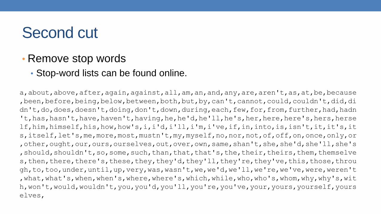
Second cut
• Remove stop words
• Stop-word lists can be found online.
a,about,above,after,again,against,all,am,an,and,any,are,aren't,as,at,be,because
,been,before,being,below,between,both,but,by,can't,cannot,could,couldn't,did,di
dn't,do,does,doesn't,doing,don't,down,during,each,few,for,from,further,had,hadn
't,has,hasn't,have,haven't,having,he,he'd,he'll,he's,her,here,here's,hers,herse
lf,him,himself,his,how,how's,i,i'd,i'll,i'm,i've,if,in,into,is,isn't,it,it's,it
s,itself,let's,me,more,most,mustn't,my,myself,no,nor,not,of,off,on,once,only,or
,other,ought,our,ours,ourselves,out,over,own,same,shan't,she,she'd,she'll,she's
,should,shouldn't,so,some,such,than,that,that's,the,their,theirs,them,themselve
s,then,there,there's,these,they,they'd,they'll,they're,they've,this,those,throu
gh,to,too,under,until,up,very,was,wasn't,we,we'd,we'll,we're,we've,were,weren't
,what,what's,when,when's,where,where's,which,while,who,who's,whom,why,why's,wit
h,won't,would,wouldn't,you,you'd,you'll,you're,you've,your,yours,yourself,yours
elves,

Second cut
• Remove stop words
• Stop-word lists can be found online.ramen 8572
pork 4152
wait 3195
good 2867
place 2361
noodles 2279
ippudo 2261
buns 2251
broth 2041
like 1902
just 1896
get 1641
time 1613
one 1460
really 1437
go 1366
food 1296
bowl 1272
can 1256
great 1172
best 1167
burger 4340
shack 3291
shake 3221
line 2397
fries 2260
good 1920
burgers 1643
wait 1508
just 1412
cheese 1307
like 1204
food 1175
get 1162
place 1159
one 1118
long 1013
go 995
time 951
park 887
can 860
best 849
sauce 4023
food 2507
cart 2239
chicken 2238
rice 2052
hot 1835
white 1782
line 1755
good 1629
lamb 1422
halal 1343
just 1338
get 1332
one 1222
like 1096
place 1052
go 965
can 878
night 832
time 794
long 792
people 790
pastrami 3782
sandwich 2934
place 1480
good 1341
get 1251
katz's 1223
just 1214
like 1207
meat 1168
one 1071
deli 984
best 965
go 961
ticket 955
food 896
sandwiches 813
can 812
beef 768
order 720
pickles 699
time 662
Commonly used words in reviews, not so interesting

IDF
• Important words are the ones that are unique to the document (differentiating) compared to the rest of the collection• All reviews use the word “like”. This is not interesting
• We want the words that characterize the specific restaurant
• Document Frequency 𝐷𝐹(𝑤): fraction of documents that contain word 𝑤.
𝐷𝐹(𝑤) =𝐷(𝑤)
𝐷
• Inverse Document Frequency 𝐼𝐷𝐹(𝑤):
𝐼𝐷𝐹(𝑤) = log1
𝐷𝐹(𝑤)
• Maximum when unique to one document : 𝐼𝐷𝐹(𝑤) = log(𝐷)• Minimum when the word is common to all documents: 𝐼𝐷𝐹(𝑤) = 0
𝐷(𝑤): num of docs that contain word 𝑤𝐷: total number of documents

TF-IDF
• The words that are best for describing a document are the ones that are
important for the document, but also unique to the document.
• 𝑇𝐹(𝑤, 𝑑): term frequency of word w in document d
• Number of times that the word appears in the document
• Natural measure of importance of the word for the document
• 𝐼𝐷𝐹(𝑤): inverse document frequency
• Natural measure of the uniqueness of the word w
• 𝑇𝐹-𝐼𝐷𝐹(𝑤, 𝑑) = 𝑇𝐹(𝑤, 𝑑) 𝐼𝐷𝐹(𝑤)

Third cut
• Ordered by TF-IDFramen 3057.41761944282 7
akamaru 2353.24196503991 1
noodles 1579.68242449612 5
broth 1414.71339552285 5
miso 1252.60629058876 1
hirata 709.196208642166 1
hakata 591.76436889947 1
shiromaru 587.1591987134 1
noodle 581.844614740089 4
tonkotsu 529.594571388631 1
ippudo 504.527569521429 8
buns 502.296134008287 8
ippudo's 453.609263319827 1
modern 394.839162940177 7
egg 367.368005696771 5
shoyu 352.295519228089 1
chashu 347.690349042101 1
karaka 336.177423577131 1
kakuni 276.310211159286 1
ramens 262.494700601321 1
bun 236.512263803654 6
wasabi 232.366751234906 3
dama 221.048168927428 1
brulee 201.179739054263 2
fries 806.085373301536 7
custard 729.607519421517 3
shakes 628.473803858139 3
shroom 515.779060830666 1
burger 457.264637954966 9
crinkle 398.34722108797 1
burgers 366.624854809247 8
madison 350.939350307801 4
shackburger 292.428306810 1
'shroom 287.823136624256 1
portobello 239.8062489526 2
custards 211.837828555452 1
concrete 195.169925889195 4
bun 186.962178298353 6
milkshakes 174.9964670675 1
concretes 165.786126695571 1
portabello 163.4835416025 1
shack's 159.334353330976 2
patty 152.226035882265 6
ss 149.668031044613 1
patties 148.068287943937 2
cam 105.949606780682 3
milkshake 103.9720770839 5
lamps 99.011158998744 1
lamb 985.655290756243 5
halal 686.038812717726 6
53rd 375.685771863491 5
gyro 305.809092298788 3
pita 304.984759446376 5
cart 235.902194557873 9
platter 139.459903080044 7
chicken/lamb 135.8525204 1
carts 120.274374158359 8
hilton 84.2987473324223 4
lamb/chicken 82.8930633 1
yogurt 70.0078652365545 5
52nd 67.5963923222322 2
6th 60.7930175345658 9
4am 55.4517744447956 5
yellow 54.4470265206673 8
tzatziki 52.9594571388631 1
lettuce 51.3230168022683 8
sammy's 50.656872045869 1
sw 50.5668577816893 3
platters 49.9065970003161 5
falafel 49.4796995212044 4
sober 49.2211422635451 7
moma 48.1589121730374 3
pastrami 1931.94250908298 6
katz's 1120.62356508209 4
rye 1004.28925735888 2
corned 906.113544700399 2
pickles 640.487221580035 4
reuben 515.779060830666 1
matzo 430.583412389887 1
sally 428.110484707471 2
harry 226.323810772916 4
mustard 216.079238853014 6
cutter 209.535243462458 1
carnegie 198.655512713779 3
katz 194.387844446609 7
knish 184.206807439524 1
sandwiches 181.415707218 8
brisket 131.945865389878 4
fries 131.613054313392 7
salami 127.621117258549 3
knishes 124.339595021678 1
delicatessen 117.488967607 2
deli's 117.431839742696 1
carver 115.129254649702 1
brown's 109.441778045519 2
matzoh 108.22149937072 1

Third cut
• TF-IDF takes care of stop words as well
• We do not need to remove the stopwords since they will get
𝐼𝐷𝐹(𝑤) = 0
• Important: IDF is collection-dependent!
• For some other corpus the words get, like, eat, may be important

Decisions, decisions…
• When mining real data you often need to make some decisions• What data should we collect? How much? For how long?
• Should we throw out some data that does not seem to be useful?
• Too frequent data (stop words), too infrequent (errors?), erroneous data, missing data, outliers
• How should we weight the different pieces of data?
• Most decisions are application dependent. Some information may be lost but we can usually live with it (most of the times)
• We should make our decisions clear since they affect our findings.
• Dealing with real data is hard…
AAAAAAAAAAAAA
AAAAAAAAAAAAAAAAAAAAAAAAA AAAAAAAAAAAAAAAAAAAAAAAAA AAAAn actual review

The preprocessing pipeline for our text mining task
Data Mining
Throw away very
short reviews
Normalize text and
break into words
Compute TF-IDF values
Keep top-k words for
each document
Remove stopwords,
very frequent words,
and very rare words
A collection of
documents as text
Subset of the
collection
Documents as
sets of words
Documents as
vectors
Documents as
subsets of words
Use Yelp/FS API
to obtain data
(or download)
Data collection
Data Preprocessing

Word and document representations
• Using TF-IDF values has a very long history in text mining
• Assigns a numerical value to each word, and a vector to a document
• Recent trend: Use word embeddings
• Map every word into a multidimensional vector
• Use the notion of context: the words that surround a word in a phrase
• Similar words appear in similar contexts
• Similar words should be mapped to close-by vectors
• Example: words “movie” and “film”
• Both words are likely to appear with similar words
• director, actor, actress, scenario, script, Oscar, cinemas etc
The actor for the movie Joker is candidate for an Oscarmovie
film
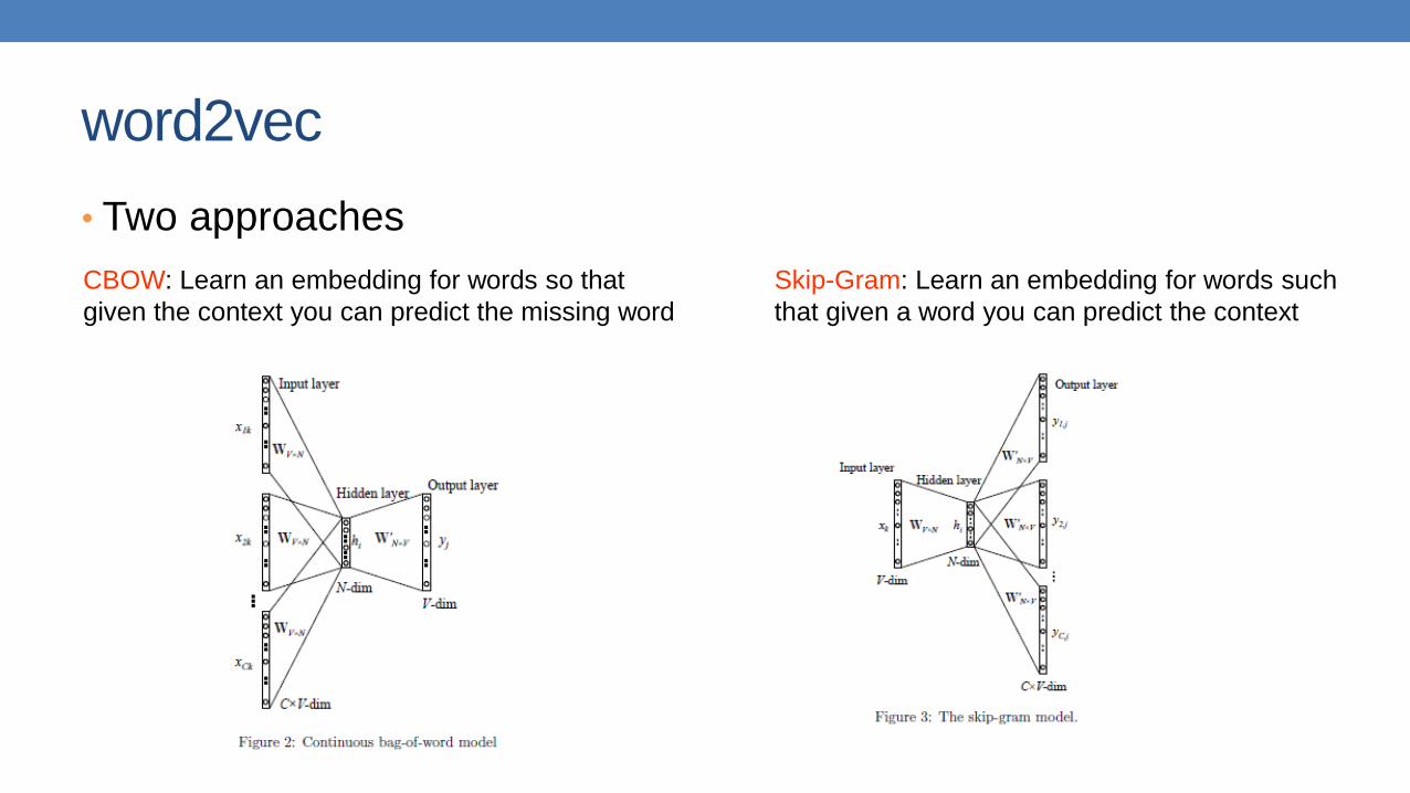
word2vec
• Two approaches
CBOW: Learn an embedding for words so that
given the context you can predict the missing word
Skip-Gram: Learn an embedding for words such
that given a word you can predict the context

Normalization of numeric data
• In many cases it is important to normalize the data rather than use
the raw values
• The kind of normalization that we use depends on what we want to
achieve

Column normalization
• In this data, different attributes take very different range of values.
For distance/similarity the small values will disappear
• We need to make them comparable
Temperature Humidity Pressure
30 0.8 90
32 0.5 80
24 0.3 95

Column Normalization
• Divide (the values of a column) by the maximum value for each
attribute
• Brings everything in the [0,1] range, maximum is 1
Temperature Humidity Pressure
0.9375 1 0.9473
1 0.625 0.8421
0.75 0.375 1
new value = old value / max value in the column
Temperature Humidity Pressure
30 0.8 90
32 0.5 80
24 0.3 95

Column Normalization
• Subtract the minimum value and divide by the difference of the
maximum value and minimum value for each attribute
• Brings everything in the [0,1] range, maximum is one, minimum is zero
Temperature Humidity Pressure
0.75 1 0.33
1 0.6 0
0 0 1
new value = (old value – min column value) / (max col. value –min col. value)
Temperature Humidity Pressure
30 0.8 90
32 0.5 80
24 0.3 95
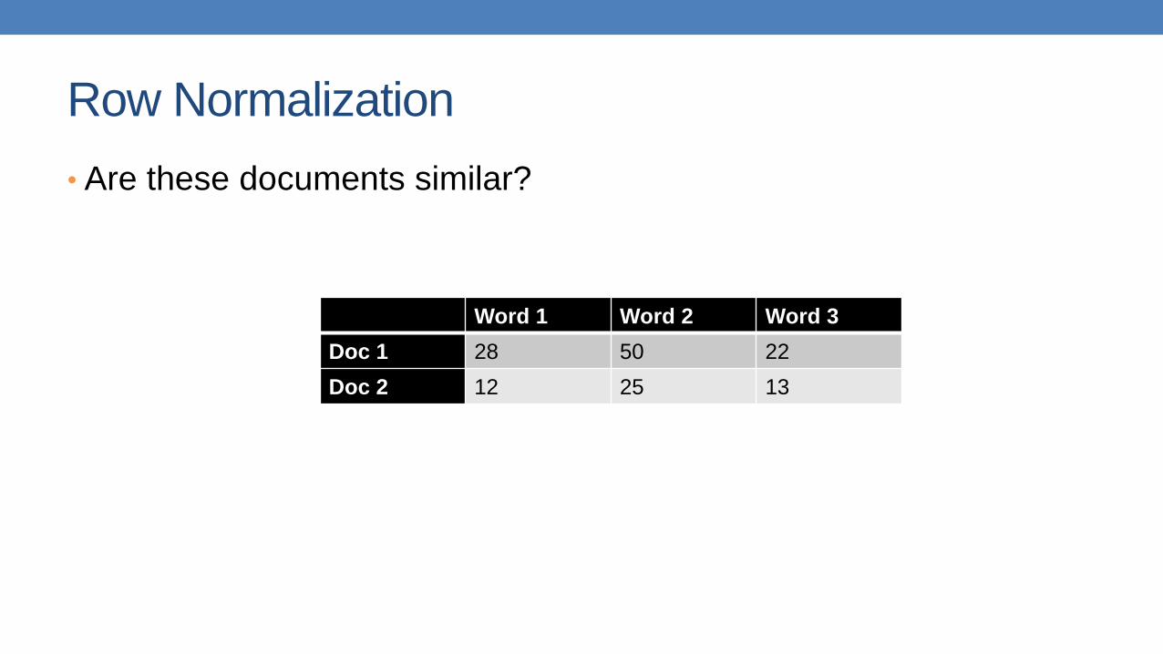
Row Normalization
• Are these documents similar?
Word 1 Word 2 Word 3
Doc 1 28 50 22
Doc 2 12 25 13

Row Normalization
• Are these documents similar?
• Divide by the sum of values for each document (row in the matrix)
• Transform a vector into a distribution*
Word 1 Word 2 Word 3
Doc 1 0.28 0.5 0.22
Doc 2 0.24 0.5 0.26
Word 1 Word 2 Word 3
Doc 1 28 50 22
Doc 2 12 25 13
new value = old value / Σ old values in the row
*For example, the value of cell (Doc1,
Word2) is the probability that a randomly
chosen word of Doc1 is Word2

Row Normalization
• Do these two users rate movies in a similar way?
Movie 1 Movie 2 Movie 3
User 1 1 2 3
User 2 2 3 4

Row Normalization
• Do these two users rate movies in a similar way?
• Subtract the mean value for each user (row) – centering of data
• Captures the deviation from the average behavior
Movie 1 Movie 2 Movie 3
User 1 -1 0 +1
User 2 -1 0 +1
Movie 1 Movie 2 Movie 3
User 1 1 2 3
User 2 2 3 4
new value = (old value – mean row value) [/ (max row value –min row value)]

Row Normalization
• Z-score:
𝑧𝑖 =𝑥𝑖 −mean(𝑥)
std(𝑥)
• Measures the number of standard deviations away from the mean
Movie 1 Movie 2 Movie 3
User 1 1.01 -0.87 -0.22
User 2 -1.01 0.55 0.93
Movie 1 Movie 2 Movie 3 Mean STD
User 1 5 2 3 3.33 1.53
User 2 1 3 4 2.66 1.53
mean 𝑥 =1
𝑁
𝑗=1
𝑁
𝑥𝑗
std 𝑥 =σ𝑗=1𝑁 𝑥𝑗 −mean 𝑥
2
𝑁
Average “distance” from the mean
N may be N-1: population vs sample

Row Normalization
• What if we want to transform the scores into probabilities?
• E.g., probability that the user will visit the restaurant again
• Different from “probability that the user will select one among the three”
• One idea: Normalize by the max score:
• Problem with that?
• We have probability 1, too strong
Restaurant 1 Restaurant 2 Restaurant 3
User 1 1 0.4 0.6
User 2 0.25 0.75 1
Restaurant 1 Restaurant 2 Restaurant 3
User 1 5 2 3
User 2 1 3 4
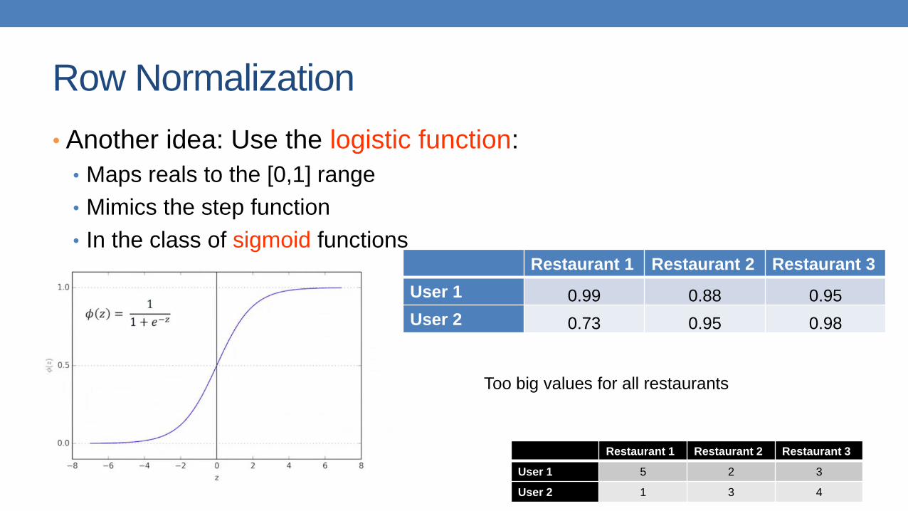
Row Normalization
• Another idea: Use the logistic function:
• Maps reals to the [0,1] range
• Mimics the step function
• In the class of sigmoid functionsRestaurant 1 Restaurant 2 Restaurant 3
User 1 0.99 0.88 0.95
User 2 0.73 0.95 0.98
Restaurant 1 Restaurant 2 Restaurant 3
User 1 5 2 3
User 2 1 3 4
Too big values for all restaurants

Row Normalization
• Another idea: Use the logistic function:
• Maps reals to the [0,1] range
• Mimics the step function
• In the class of sigmoid functionsRestaurant 1 Restaurant 2 Restaurant 3
User 1 0.99 0.88 0.95
User 2 0.73 0.95 0.98
Restaurant 1 Restaurant 2 Restaurant 3
User 1 5 2 3
User 2 1 3 4
Subtract the mean
Mean value gets 50-50 probability

Row Normalization
• General sigmoid function:
• We can control the zero point and the slope
Higher 𝑐1closer to
a step function
𝑐2 controls the 0.5 point
– change of slope

Row Normalization
• What if we want to transform the scores into probabilities that sum
to one, but we capture the single selection of the user?
• Use the softmax function𝑒𝑥𝑖
σ𝑖 𝑒𝑥𝑖
Restaurant 1 Restaurant 2 Restaurant 3
User 1 0.72 0.10 0.18
User 2 0.07 0.31 0.62
Restaurant 1 Restaurant 2 Restaurant 3
User 1 5 2 3
User 2 1 3 4

Exploratory analysis of data
• Summary statistics: numbers that summarize properties of the data
• Summarized properties include frequency, location and spread
• Examples: location - meanspread - standard deviation
• Most summary statistics can be calculated in a single pass through the data
• Computing data statistics is one of the first steps in understanding our data

Frequency and Mode
• The frequency of an attribute value is the percentage of time the
value occurs in the data set
• For example, given the attribute ‘gender’ and a representative population of
people, the gender ‘female’ occurs about 50% of the time.
• The mode of an attribute is the most frequent attribute value
• The notions of frequency and mode are typically used with categorical data
• We can visualize the data frequencies using a value histogram
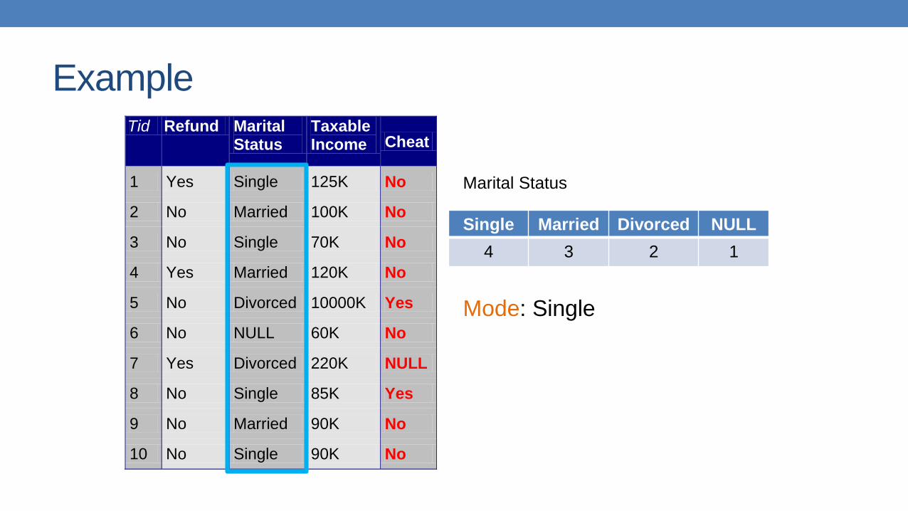
ExampleTid Refund Marital
Status Taxable Income Cheat
1 Yes Single 125K No
2 No Married 100K No
3 No Single 70K No
4 Yes Married 120K No
5 No Divorced 10000K Yes
6 No NULL 60K No
7 Yes Divorced 220K NULL
8 No Single 85K Yes
9 No Married 90K No
10 No Single 90K No 10
Single Married Divorced NULL
4 3 2 1
Marital Status
Mode: Single

ExampleTid Refund Marital
Status Taxable Income Cheat
1 Yes Single 125K No
2 No Married 100K No
3 No Single 70K No
4 Yes Married 120K No
5 No Divorced 10000K Yes
6 No NULL 60K No
7 Yes Divorced 220K NULL
8 No Single 85K Yes
9 No Married 90K No
10 No Single 90K No 10
Marital Status
Single Married Divorced NULL
40% 30% 20% 10%

ExampleTid Refund Marital
Status Taxable Income Cheat
1 Yes Single 125K No
2 No Married 100K No
3 No Single 70K No
4 Yes Married 120K No
5 No Divorced 10000K Yes
6 No NULL 60K No
7 Yes Divorced 220K NULL
8 No Single 85K Yes
9 No Married 90K No
10 No Single 90K No 10
Marital Status
Single Married Divorced
44% 33% 22%
0
0.1
0.2
0.3
0.4
0.5
Single Married Divorced
Marital Status
We can choose to ignore NULL values

Data histograms
Tid Refund Marital Status
Taxable Income Cheat
1 Yes Single 125K No
2 No Married 100K No
3 No Single 70K No
4 Yes Married 120K No
5 No Divorced 10000K Yes
6 No NULL 60K No
7 Yes Divorced 220K NULL
8 No Single 85K Yes
9 No Married 90K No
10 No Single 90K No 10
0
0.1
0.2
0.3
0.4
0.5
0.6
0.7
0.8
Yes No
Refund
0
0.1
0.2
0.3
0.4
0.5
Single Married Divorced
Marital Status
0
0.1
0.2
0.3
0.4
0.5
0.6
<100K [100K,200K] >200K
Income
Use binning for numerical values
50%
30%
20%
INCOME
<100K [100K,200K] >200K
45%
33%
22%
Marital Status
Single Married Divorced
Yes
No
REFUND

Percentiles
• For continuous data, the notion of a percentile is more useful.
Given an ordinal or continuous attribute x and a number p between 0
and 100, the pth percentile is a value 𝑥𝑝 of x such that p% of the
observed values of x are less or equal than 𝑥𝑝.
• For instance, the 80th percentile is the value 𝑥80% that is greater or
equal than 80% of all the values of x we have in our data.

ExampleTid Refund Marital
Status Taxable Income Cheat
1 Yes Single 125K No
2 No Married 100K No
3 No Single 70K No
4 Yes Married 120K No
5 No Divorced 10000K Yes
6 No NULL 60K No
7 Yes Divorced 220K NULL
8 No Single 85K Yes
9 No Married 90K No
10 No Single 90K No 10
Taxable
Income
10000K
220K
125K
120K
100K
90K
90K
85K
70K
60K
𝑥80% = 125K

Measures of Location: Mean and Median
• The mean is the most common measure of the location of a set of
points.
• However, the mean is very sensitive to outliers.
• Thus, the median or a trimmed mean is also commonly used.

ExampleTid Refund Marital
Status Taxable Income Cheat
1 Yes Single 125K No
2 No Married 100K No
3 No Single 70K No
4 Yes Married 120K No
5 No Divorced 10000K Yes
6 No NULL 60K No
7 Yes Divorced 220K NULL
8 No Single 85K Yes
9 No Married 90K No
10 No Single 90K No 10
Mean: 1090K
Trimmed mean (remove min, max): 105K
Median: (90+100)/2 = 95K

Measures of Spread: Range and Variance
• Range is the difference between the max and min
• The variance or standard deviation is the most common measure of the spread of a set of points.
𝑣𝑎𝑟 𝑥 =1
𝑚
𝑖=1
𝑚
𝑥 − ҧ𝑥 2
𝜎 𝑥 = 𝑣𝑎𝑟 𝑥
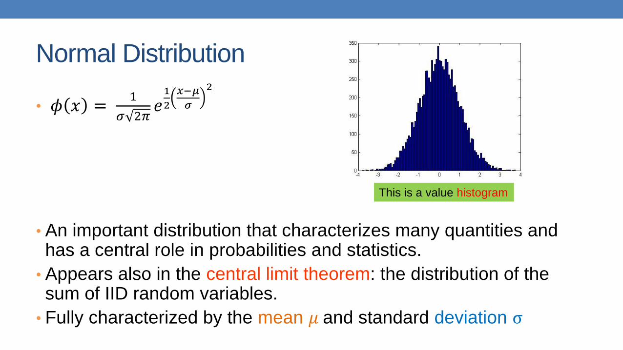
Normal Distribution
• 𝜙 𝑥 =1
𝜎 2𝜋𝑒1
2
𝑥−𝜇
𝜎
2
• An important distribution that characterizes many quantities and has a central role in probabilities and statistics.
• Appears also in the central limit theorem: the distribution of the sum of IID random variables.
• Fully characterized by the mean 𝜇 and standard deviation σ
This is a value histogram

Not everything is normally distributed
• Plot of number of words with x number of occurrences
• If this was a normal distribution we would not have number of
occurrences as large as 28K
0
1000
2000
3000
4000
5000
6000
7000
8000
0 5000 10000 15000 20000 25000 30000 35000
y: number of
words with x
number of
occurrences
x: number of occurrences

Power-law distribution
• We can understand the distribution of words if we take the log-log plot
1
10
100
1000
10000
1 10 100 1000 10000 100000
The slope of the line
gives us the
exponent α
y: logarithm of
number of words
with x number of
occurrences
x: logarithm of number of occurrences
Linear relationship in the log-log space
log 𝑝 𝑥 = 𝑘 = −𝑎 log 𝑘
Power-law distribution:
𝑝 𝑘 = 𝑘−𝑎

Power-laws are everywhere
• Incoming and outgoing links of web pages, number of friends in
social networks, number of occurrences of words, file sizes, city
sizes, income distribution, popularity of products and movies
• Signature of human activity?
• A mechanism that explains everything?
• Rich get richer process

Zipf’s law
• Power laws can be detected also by a linear relationship in the log-log space for the rank-frequency plot
• 𝑓 𝑟 : Frequency of the r-th most frequent word
log 𝑓 𝑟 = −𝛽 log 𝑟
1
10
100
1000
10000
100000
1 10 100 1000 10000 100000
r: rank of word according to frequency (1st, 2nd …)
y: number of
occurrences of the r-th
most frequent wordZipf distribution:
𝑓 𝑟 = 𝑟−𝛽

The importance of correct representation
• Consider the following three plots which are histograms of values. What do
you observe? What can you tell of the underlying function?
0
0.1
0.2
0.3
0.4
0.5
0.6
0.7
0.8
0 20 40 60 80 100
0
0.05
0.1
0.15
0.2
0.25
0.3
0.35
0.4
0 20 40 60 80 100
0
0.1
0.2
0.3
0.4
0.5
0.6
0.7
0.8
0.9
1
0 20 40 60 80 100

The importance of correct representation
• Putting all three plots together makes it clearer to see the differences
• Green falls more slowly. Blue and Red seem more or less the same
0
0.1
0.2
0.3
0.4
0.5
0.6
0.7
0.8
0.9
1
0 20 40 60 80 100
Series1
Series2
Series3

The importance of correct representation
• Making the plot in log-log space makes the differences more clear
• Green and Blue form straight lines. Red drops exponentially.
• 𝑦 =1
2𝑥+𝜖log 𝑦 ≈ − log 𝑥 + 𝑐
• 𝑦 =1
𝑥2+𝜖log 𝑦 ≈ −2 log 𝑥 + 𝑐
• 𝑦 = 2−𝑥 + 𝜖 log 𝑦 ≈ −𝑥 + 𝑐 = −10log 𝑥 + 𝑐
1E-30
1E-28
1E-26
1E-24
1E-22
1E-20
1E-18
1E-16
1E-14
1E-12
1E-10
1E-08
1E-06
0.0001
0.01
1
1 10 100
Series1
Series2
Series3
Linear relationship in log-log
means polynomial in linear-linear
The slope in the log-log is the
exponent of the polynomial

Attribute relationships
• In many cases it is interesting to look at two attributes together to
understand if they are correlated
• E.g., how does your marital status relate with tax cheating?
• E.g., Does refund correlate with average income?
• Is there a relationship between years of study and income?
• How do we visualize these relationships?

Plotting attributes against each other
Tid Refund Marital Status
Taxable Income Cheat
1 Yes Single 125K No
2 No Married 100K No
3 No Single 70K No
4 Yes Married 120K No
5 No Divorced 10000K Yes
6 No Married 60K No
7 Yes Divorced 220K No
8 No Single 85K Yes
9 No Married 90K No
10 No Single 90K No 10
No Yes
Single 2 1
Married 4 0
Divorced 1 1
Confusion Matrix
No Yes
Single 0.2 0.1
Married 0.4 0.0
Divorced 0.1 0.1
Joint Distribution Matrix
No Yes
Single 0.2 0.1
Married 0.4 0.0
Divorced 0.1 0.1

Plotting attributes against each other
Tid Refund Marital Status
Taxable Income Cheat
1 Yes Single 125K No
2 No Married 100K No
3 No Single 70K No
4 Yes Married 120K No
5 No Divorced 10000K Yes
6 No Married 60K No
7 Yes Divorced 220K No
8 No Single 85K Yes
9 No Married 90K No
10 No Single 90K No 10
No Yes
Single 0.2 0.1 0.3
Married 0.4 0.0 0.4
Divorced 0.1 0.1 0.2
0.8 0.2 1
Joint Distribution Matrix
Marginal
distribution
for Marital
Status
Marginal distribution
for Cheat

Plotting attributes against each other
Tid Refund Marital Status
Taxable Income Cheat
1 Yes Single 125K No
2 No Married 100K No
3 No Single 70K No
4 Yes Married 120K No
5 No Divorced 10000K Yes
6 No Married 60K No
7 Yes Divorced 220K No
8 No Single 85K Yes
9 No Married 90K No
10 No Single 90K No 10
No Yes
Single 0.2 0.1 0.3
Married 0.4 0.0 0.4
Divorced 0.1 0.1 0.2
0.8 0.2 1
Joint Distribution Matrix P
No Yes
Single 0.24 0.06 0.3
Married 0.32 0.08 0.4
Divorced 0.16 0.04 0.2
0.8 0.2 1
Independence Matrix E
How do we know if there are interesting correlations?
The product of the
two marginal
values 0.2*0.8
Compare the values 𝑃𝑥𝑦 with 𝐸𝑥𝑦

Plotting attributes against each other
Tid Refund Marital Status
Taxable Income Cheat
1 Yes Single 125K No
2 No Married 100K No
3 No Single 70K No
4 Yes Married 120K No
5 No Divorced 10000K Yes
6 No Married 60K No
7 Yes Divorced 220K No
8 No Single 85K Yes
9 No Married 90K No
10 No Single 90K No 10
No Yes
Single 0.2 0.1 0.3
Married 0.4 0.0 0.4
Divorced 0.1 0.1 0.2
0.8 0.2 1
Joint Distribution Matrix P
No Yes
Single 0.24 0.06 0.3
Married 0.32 0.08 0.4
Divorced 0.16 0.04 0.2
0.8 0.2 1
Independence Matrix E
We can compare specific pairs of values:
• If 𝑃 𝑥, 𝑦 > 𝐸(𝑥, 𝑦) there is positive correlation (e.g, Married, No)
• If 𝑃 𝑥, 𝑦 < 𝐸(𝑥, 𝑦) there is negative correlation (e.g., Single, No)
• Otherwise there is no correlation
The quantity 𝑃(𝑥,𝑦)
𝐸(𝑥,𝑦)=
𝑃(𝑥,𝑦)
𝑃 𝑥 𝑃(𝑦)is called Lift, or Pointwise Mutual Information

Plotting attributes against each other
Tid Refund Marital Status
Taxable Income Cheat
1 Yes Single 125K No
2 No Married 100K No
3 No Single 70K No
4 Yes Married 120K No
5 No Divorced 10000K Yes
6 No Married 60K No
7 Yes Divorced 220K No
8 No Single 85K Yes
9 No Married 90K No
10 No Single 90K No 10
No Yes
Single 0.2 0.1 0.3
Married 0.4 0.0 0.4
Divorced 0.1 0.1 0.2
0.8 0.2 1
Joint Distribution Matrix P
No Yes
Single 0.24 0.06 0.3
Married 0.32 0.08 0.4
Divorced 0.16 0.04 0.2
0.8 0.2 1
Independence Matrix E
Or compare the two attributes:
Pearson 𝑥2 Independence Test Statistic:
𝑈 = 𝑁
𝑥
𝑦
𝑃𝑥𝑦 − 𝐸𝑥𝑦2
𝐸𝑥𝑦

Hypothesis testing
• How important is the statistic value we computed?
• Formulate a null hypothesis 𝐻0:• 𝐻0 = the two attributes are independent
• Compute the distribution of the statistic in the case that 𝐻0 is true• In this case we can show that the statistic 𝑈 follows a 𝜒2 distribution
• For the statistic value 𝜃 we computed, compute the probability 𝑃(𝑈 > 𝜃)under the null hypothesis• For most distributions there are tables that give these numbers for our data
• This is the p-value of our experiment:
• We want it to be small• This means that the observed value is interesting
The p-value is the probability (under 𝐻0) of observing a value of the test statistic the
same as, or more extreme than what was actually observed

Categorical and numerical attributes
Tid Refund Marital Status
Taxable Income Cheat
1 Yes Single 125K No
2 No Married 100K No
3 No Single 70K No
4 Yes Married 120K No
5 No Divorced 10000K Yes
6 No NULL 60K No
7 Yes Divorced 220K NULL
8 No Single 85K Yes
9 No Married 90K No
10 No Single 90K No 10
0
200
400
600
800
1000
1200
1400
1600
Yes No
Ave
rag
e I
nco
me
Refund
Average Income vs Refund

Categorical and numerical attributes
Tid Refund Marital Status
Taxable Income Cheat
1 Yes Single 125K No
2 No Married 100K No
3 No Single 70K No
4 Yes Married 120K No
5 No Divorced 10000K Yes
6 No NULL 60K No
7 Yes Divorced 220K NULL
8 No Single 85K Yes
9 No Married 90K No
10 No Single 90K No 10
After removing the outlier value
0
20
40
60
80
100
120
140
160
180
Yes No
Avera
ge Incom
e
Refund
Average Income vs Refund
Is this difference significant?

Categorical and numerical attributes
Tid Refund Marital Status
Taxable Income Cheat
1 Yes Single 125K No
2 No Married 100K No
3 No Single 70K No
4 Yes Married 120K No
5 No Divorced 10000K Yes
6 No NULL 60K No
7 Yes Divorced 220K NULL
8 No Single 85K Yes
9 No Married 90K No
10 No Single 90K No 10
Compute error bars
0
50
100
150
200
250
Yes No
Ave
rag
e I
nco
e
Refund
Average Income vs Refund
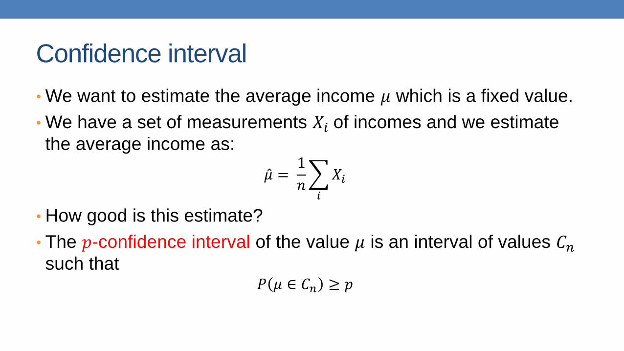
Confidence interval
• We want to estimate the average income 𝜇 which is a fixed value.
• We have a set of measurements 𝑋𝑖 of incomes and we estimate
the average income as:
Ƹ𝜇 =1
𝑛
𝑖
𝑋𝑖
• How good is this estimate?
• The 𝑝-confidence interval of the value 𝜇 is an interval of values 𝐶𝑛such that
𝑃 𝜇 ∈ 𝐶𝑛 ≥ 𝑝

Standard error
• If we have a measurement 𝜃 that we estimate from the data, the standard error is defined as
𝑠𝑒 = 𝑉𝑎𝑟( 𝜃)
• In our case our measurement is the average income which we estimate as:
Ƹ𝜇 =1
𝑛
𝑖
𝑋𝑖
• We assume that 𝑋𝑖 are independent samples of the income random variable 𝑋 that come from the same distribution. We can show that:
𝑠𝑒 =𝑉𝑎𝑟(𝑋)
𝑛• We can estimate 𝑉𝑎𝑟(𝑋) from the data
• The value ො𝜇 follows a normal distribution for large 𝑛. For normal distributions the 95% confidence interval for the real average income 𝜇 is:
Ƹ𝜇 − 2𝑠𝑒, Ƹ𝜇 + 2𝑠𝑒
We use the fact that:
𝑉𝑎𝑟
𝑖
𝛼𝑖𝑋𝑖 =
𝑖
𝛼𝑖2𝑉𝑎𝑟(𝑋𝑖)

Statistical tests
• There are statistical tests for testing if two samples come from distributions with the same mean (or median)
• These tests can also provide us with a p-value
• Wald test:• Tests the null hypothesis that our variable takes a specific value
• E.g., the difference of the means or medians is zero
• Student t-test:• Test of the means of two normal distributions
• Permutation test:• Sample permutations of the merged data points and compute an empirical
p-value

Correlating numerical attributes
Tid Refund Marital Status
Taxable Income
Years of Study
1 Yes Single 125K 4
2 No Married 100K 5
3 No Single 70K 3
4 Yes Married 120K 3
5 No Divorced 10000K 6
6 No NULL 60K 1
7 Yes Divorced 220K 8
8 No Single 85K 3
9 No Married 90K 2
10 No Single 90K 4 10
0
2000
4000
6000
8000
10000
12000
0 2 4 6 8 10
Inco
me
Years of Study
Income vs Years of study
Scatter plot:
X axis is one attribute, Y axis is the other
For each entry we have two values
Plot the entries as two-dimensional points

Plotting attributes against each other
Tid Refund Marital Status
Taxable Income
Years of Study
1 Yes Single 125K 4
2 No Married 100K 5
3 No Single 70K 3
4 Yes Married 120K 3
5 No Divorced 10000K 6
6 No NULL 60K 1
7 Yes Divorced 220K 8
8 No Single 85K 3
9 No Married 90K 2
10 No Single 90K 4 10
After removing the outlier value there is a clear correlation
0
50
100
150
200
250
0 2 4 6 8 10
Inco
me
Years of Study
Income vs Years of Study
Scatter plot:
X axis is one attribute, Y axis is the other
For each entry we have two values
Plot the entries as two-dimensional points

Scatter Plot Array of Iris Attributes

Measuring correlation
• Pearson correlation coefficient: measures the extent to which two variables are linearly correlated
• 𝑋 = 𝑥1, … , 𝑥𝑛• 𝑌 = 𝑦1, … , 𝑦𝑛
• 𝑐𝑜𝑟𝑟 𝑋, 𝑌 =σ𝑖(𝑥𝑖−𝜇𝑋)(𝑦𝑖−𝜇𝑌)
σ𝑖 𝑥𝑖−𝜇𝑋2 σ𝑖 𝑦𝑖−𝜇𝑌
2
• It comes with a p-value• The p-value is the probability that the correlation was by chance.
• Assumes no outliers and that the variables are normally distributed
• Spearman rank correlation coefficient: tells us if two variable are rank-correlated• They place items in the same order – Pearson correlation of the rank vectors
• For ranking without ties it looks at the differences between the ranks of the same items
Must have pairs of observations

Post-processing
• Visualization
• The human eye is a powerful analytical tool
• If we visualize the data properly, we can discover patterns and demonstrate
trends
• Visualization is the way to present the data so that patterns can be seen
• E.g., histograms and plots are a form of visualization
• There are multiple techniques (a field on its own)

Visualization on a map
• John Snow, London 1854

Charles Minard map
Six types of data in one plot: size of army, temperature, direction, location, dates etc

Another interesting visualization
• China growth over the years

Dimensionality Reduction
• The human eye is limited to processing visualizations in two (at
most three) dimensions
• One of the great challenges in visualization is to visualize high-
dimensional data into a two-dimensional space
• Dimensionality reduction
• Distance preserving embeddings
• Dimensionality reduction is also a preprocessing technique:
• Reduce the amount of data
• Extract the useful information.

Example
• Consider the following 6-dimensional dataset
𝐷 =
1 2 32 4 60 0 0
0 0 00 0 01 2 3
0 0 01 2 32 4 6
2 4 61 2 32 4 6
• What do you observe? Can we reduce the dimension of the data?

Example𝐷 =
1 2 32 4 60 0 0
0 0 00 0 01 2 3
0 0 01 2 32 4 6
2 4 61 2 32 4 6
• Each row is a multiple of two vectors
• 𝑥 = 1, 2, 3, 0, 0, 0
• 𝑦 = [0, 0, 0, 1, 2, 3]
• We can rewrite 𝐷 as
𝐷 =
1 02 00 10 21 12 2 Three types of data points

Word Clouds
• A fancy way to visualize a document or collection of documents.

Heatmaps
• Plot a point-to-point similarity matrix using a heatmap:
• Deep red = high values (hot)
• Dark blue = low values (cold)
0 0.2 0.4 0.6 0.8 10
0.1
0.2
0.3
0.4
0.5
0.6
0.7
0.8
0.9
1
x
y
Points
Po
ints
20 40 60 80 100
10
20
30
40
50
60
70
80
90
100Similarity
0
0.1
0.2
0.3
0.4
0.5
0.6
0.7
0.8
0.9
1
The clustering structure becomes clear in the heatmap

Heatmaps
• Heatmap (grey scale) of the data matrix
• Document-word frequenciesD
ocum
ents
Words
Before clustering After clustering

Heatmaps
A very popular way to visualize data
http://projects.oregonlive.com/ucc-shooting/gun-deaths.php

Statistical Significance
• When we extract knowledge from a large dataset we need to make
sure that what we found is not an artifact of randomness
• E.g., we find that many people buy milk and toilet paper together.
• But many (more) people buy milk and toilet paper independently
• Statistical tests compare the results of an experiment with those
generated by a null hypothesis
• E.g., a null hypothesis is that people select items independently.
• A result is interesting if it cannot be produced by randomness.
• An important problem is to define the null hypothesis correctly: What is
random?

136
Meaningfulness of Answers
• A big data-mining risk is that you will “discover” patterns that are
meaningless.
• Statisticians call it Bonferroni’s principle: (roughly) if you look in
more places for interesting patterns than your amount of data will
support, you are bound to find crap.
• The Rhine Paradox: a great example of how not to conduct
scientific research.
CS345A Data Mining on the Web: Anand Rajaraman, Jeff Ullman

137
Rhine Paradox – (1)
• Joseph Rhine was a parapsychologist in the 1950’s who
hypothesized that some people had Extra-Sensory Perception.
• He devised (something like) an experiment where subjects were
asked to guess 10 hidden cards – red or blue.
• He discovered that almost 1 in 1000 had ESP – they were able to
get all 10 right!
CS345A Data Mining on the Web: Anand Rajaraman, Jeff Ullman

138
Rhine Paradox – (2)
• He told these people they had ESP and called them in for another
test of the same type.
• Alas, he discovered that almost all of them had lost their ESP.
• Why?
• What did he conclude?
• Answer on next slide.
CS345A Data Mining on the Web: Anand Rajaraman, Jeff Ullman

139
Rhine Paradox – (3)
• He concluded that you shouldn’t tell people they have ESP; it
causes them to lose it.
CS345A Data Mining on the Web: Anand Rajaraman, Jeff Ullman