Data Quality Monitoring Anomaly Detection

HAL Id: hal-03159873https://hal.inria.fr/hal-03159873

Submitted on 6 Mar 2021

HAL is a multi-disciplinary open accessarchive for the deposit and dissemination of sci-entific research documents, whether they are pub-lished or not. The documents may come fromteaching and research institutions in France orabroad, or from public or private research centers.

L’archive ouverte pluridisciplinaire HAL, estdestinée au dépôt et à la diffusion de documentsscientifiques de niveau recherche, publiés ou non,émanant des établissements d’enseignement et derecherche français ou étrangers, des laboratoirespublics ou privés.

Data Quality Monitoring Anomaly DetectionAdrian Pol, Cécile Germain, Maurizio Pierini, Gianluca Carminara

To cite this version:Adrian Pol, Cécile Germain, Maurizio Pierini, Gianluca Carminara. Data Quality MonitoringAnomaly Detection. Artificial Intelligence for High Energy Physics, In press, �10.1142/12200�. �hal-03159873�

https://hal.inria.fr/hal-03159873

https://hal.archives-ouvertes.fr

March 4, 2021 16:42 ws-rv9x6 Book Title output page 1

Chapter 1

Data Quality Monitoring

Anomaly Detection

1. Introduction

At the Large Hadron Collider (LHC), the physics data acquisition is a mul-

tiple steps process, which involves very complex and large hardware (both

detector and accelerator) and software systems. The detector components

collect raw data about the interaction of the particles with the sensitive

layers and the trigger system discards the vast majority of bunch collisions.

Due to the size and complexity of these systems, transitory or permanent

failures of components are unavoidable. Such failures produce erroneous

data. Stringent quality criteria must be imposed so that only certifiably

good data are passed further to physics analysis. This certification process

is called data quality monitoring (DQM) and is a long-established vital pro-

cedure in any modern large-scale High Energy Physics (HEP) experiment.

Failures are not only unavoidable but relatively frequent. For instance,

10%a of the detector components may manifest problems, while 2%b of the

acquired data is discarded. The relatively high figure of detector compo-

nents failures is not mostly due to significant, easily detectable, malfunc-

tions of the detector as a whole, but to localized problems. Thanks to the

essential redundancy in the detector, in most cases, entirely relevant physics

analysis can still be achieved on the data taken by the not-faulty parts of

the detector. However, all operational imperfections must be annotated.

Thus, a critical goal of the monitoring system, besides the sensitivity, is to

be as specific as possible in spotting the defects.

The ever increasing detector complexity and the volume of monitoring

data call for a paradigm shift in HEP monitoring, as the techniques in

use are swiftly reaching their limits. Machine learning (ML) techniques

promise a breakthrough, towards gradually automating the DQM scrutiny

and extending the monitoring coverage.

aCalculations are based on the CMS drift tube sub-detector data [1].bCalculations are based on the CMS data certification procedure [2].

1


2

The successes of the neural networks in quality control applications

encourage its application to other, more sensitive challenges in HEP, e.g.

searches of physics beyond the standard model [?].

The goal of this chapter is to explore how ML methods of anomaly

detection can help improving the existing DQM pipeline, under the specific

contraints derived from the critical role of data validation: interpretability

of the results, and long-term maintainability of the system.

To be concrete, we will mostly consider case studies from the CMS

DQM. However, the general setting and the challenges are very similar in

the other LHC experiments. For more details, see [3–5] for the presentation

of ATLAS, LHCb and ALICE DQM procedures.

The chapter presents increasingly difficult use cases. In summary, we

show that anomaly detection methods based on deep learning are both

efficient and effective. The proposed methods are precisely spotting the

problematic data and provide some level of interpretability, making them

acceptable to the DQM production system.

The rest of the chapter is organized as follows. Section 2 provides a

general outline of the CMS-DQM pipeline, followed by a short survey on

ML anomaly detection in Section 3. Then, we present the use cases. They

can be divided into two groups. In the first one, the main difficulty is to

model the problem, based on domain knowledge. Here, standard tools and

techniques, i.e. CNNs (Section 4.1), deep autoencoders (Section 4.2, 4.3

and 5) and LSTMs (Section 7) suffice. In contrast to these, we will also

cover a use case corresponding to an open issue for ML research: adapt-

ing the recent developments in variational inference to anomaly detection

(Section 6).

2. Data Quality Monitoring for the LHC experiments

In this section, we overview the DQM scrutiny in the LHC experiments.

We focus on the CMS experiment as we are most familiar with it. For

showing a full picture, the final Section 2.5 presents an out of experiment

example of monitoring the accelerator complex.

2.1. Overview

The LHC physics analyses are performed only on good-quality data coming

from the LHC collisions. Hence, prompt and accurate identification and

flagging of the problematic data is required. In the CMS collaboration,


Data Quality Monitoring Anomaly Detection 3

imposing quality criteria is performed by the two main domains of the

monitoring chain.

• Online monitoring provides live feedback on the quality of the data

while they are being acquired, allowing the operator crew to react

to unforeseen issues identified by the monitoring application.

• Offline monitoring, also referred to as data certification was de-

signed to certify the quality of the data collected and stored on

disk using centralized processing (referred to as the event recon-

struction, that converts detector hits into a list of detected parti-

cles, each associated with energy and direction).

The first online step is a prerequisite to an offline phase, in which detec-

tor experts monitor the data collected in a given period (typically a week)

and decide which portion of the collected dataset meeting acceptance cri-

teria. However, the two validation steps differ in three main aspects.

• The latency of the evaluation process. Online monitoring is re-

quired to identify anomalies in quasi-real-time to allow the opera-

tors to intervene promptly while the offline procedure has a typical

timescale of several days.

• The fraction of the data which they have access to. Generally,

CMS online processing runs at a rate of 100 Hz, corresponding

to approximately 10% of the data written to disk for analysis (in

order not to flood the monitoring system). The offline processing

takes as input the full set of events accepted by the trigger system

(∼ 1 kHz of collisions).

• The granularity of the monitored detector components. While

offline monitoring requires identifying the only overall status of

the sub-detectors, online should determine faulty sub-detector ele-

ments.

Despite their specific characteristics, these two steps rely on the same

failure detection strategy: the scrutiny of a long list of predefined statis-

tical tests, selected to detect a set of possible known failure modes. The

results of these tests are presented as a set of multidimensional histograms

(mostly one-dimensional) for experts’ convenience. The experts compare

each distribution to a corresponding reference, derived from good-quality

data in line with predetermined validation guidelines. The good-quality

data comes from the periods of the detector operating without any prob-

lems. The experts also look for unexpected effects that could affect analysis


4

level quantities, e.g. noise spikes, dead areas of detector problematic cali-

brations.

2.2. Experiment online legacy methods: the example of CMS

drift tubes

The CMS failure detection algorithms focus on the interpretation of detec-

tor data organized in the form of histograms. The CMS DQM visualization

tool, described in [6], displays those histograms organized geographically.

The anomaly detection performed by the experts is very often related to

identifying and discriminating healthy patterns from problematic ones. If

such regions appear during the detector operation, the collaboration needs

to know precisely when the problem appeared and how to intervene. Detec-

tor experts input their knowledge of the detector into binary classification

algorithms targeting common and foreseen failure scenarios.

A class of these problems is based on counting the number of electronic

hits per read-out channel. A concrete example could be the data recorded

by the CMS drift tube (DT) chambers of the muon spectrometer, outlined

in Figure 1. It is an excellent illustration of an approach widely used by the

CMS sub-detector communities and is referred to as occupancy monitoring.

The DT occupancy matrix can be viewed as a varying size two-

dimensional array organized with a layer (row) and channel (column) in-

dices. The method used in the online monitoring production system targets

a specific failure scenario, by far the most frequent: a region of cells not pro-

viding any electronic signal, large enough to affect the track reconstruction

in the chamber. It is usually related to temporary problems in the readout

electronics. Examples of this kind of failures are shown in Figure 1 B and C.

The legacy strategy simply counts the area of dead (yielding exactly zero

hits) regions without considering spatial proximity information. The strat-

egy evaluates samples for each one of 250 DT chambers and assembles

them in so-called summary plots. In this manner, human shifter, i.e. a

trained expert monitoring plots in real time, has a broad overview of the

sub-detector status in one or a few plots. The first response human decision

is based on the summary plot but the plot information is determined by an

algorithm, such as the one described above, subject to performance fluctu-

ations due to, for example, changing running conditions. For instance, the

DT legacy occupancy monitoring strategy regards Figure 1 instance A as

non-problematic, correctly classifies the chamber in Figure 1 B as anoma-

lous, but it is not sensitive enough to flag the chamber in Figure 1 C.



The current level of automation extends to the infrastructure that cre-

ates the plots and the superposition to the existing reference. For some sub-

detectors, a statistical test (e.g. Kolmogorov-Smirnov, χ2) is performed,

but the interpretation and ultimate decision are again taken by the human

shifter.

A

0 10 20 30 40 50Channel

1

5

9

Laye

r

coun

ts

CMS

0

104Run: 272011, W: 1.0, St: 1.0, Sec: 6.0

B

0 10 20 30 40 50 60Channel

159

Laye

r

coun

ts

CMS

0

120Run: 275310, W: 1.0, St: 2.0, Sec: 7.0

C

0 10 20 30 40 50 60Channel

159

Laye

r

coun

ts

CMS

0

28Run: 273158, W: 0.0, St: 2.0, Sec: 12.0

Figure 1. Example of visualization of occupancy data for three CMS DT chambers.

The data in (A) manifest the expected behaviour despite having a dead channel in layer1. The chamber in the plot in (B) instead shows regions of low occupancy across the 12

layers and should be classified as faulty. (C) suffers from a region in layer 1 with lower

efficiency, which should be identified as anomalous. From [1].

2.3. Legacy trigger rate monitoring

A further category of online monitoring is trigger rate monitoring. The trig-

ger system is an essential part of the LHC acquisition process and the start

of the physics event selection process. The LHC operates at the remarkable

collision rate of 40 MHz and each event corresponds up to several MBs of


6

data in unprocessed form. Due to understandable storage constraints and

technological limitations, each experiment is required to reduce the number

of recorded data.

At CMS, a hierarchical set of trigger algorithms [7] are designed to

reduce the event rate while preserving the physics reach of the experiment.

The CMS trigger system is structured in two stages using an increasingly

complex information and more refined algorithms. The Level 1 (L1) Trigger

is implemented on custom electronics and reduces the 40 MHz input to

a 100 kHz rate. High Level Trigger (HLT) is a collision reconstruction

software running on a computer farm, which scales the 100 kHz rate output

of L1 Trigger down to 1 kHz. The HLT nodes (or paths) are seeded by the

events selected by a set of L1 Trigger outputs.

The event acceptance rate is affected in the presence of several issues e.g.

detector malfunctions. Depending on the nature of the problem, the rate

associated with specific paths could change to unacceptable levels. In such

cases, the system should alert the shift crew, calling for problem diagnosis

and intervention. Critical cases include dropping to zero or increasing to

extreme values.

The rate of the physics processes determining the trigger rate decreases

with the luminosity and, as a consequence, with pile-up (PU), a number

of proton-proton collisions in the same event. Consequently, the recorded

collision rates decrease as well as they primarily depend on the luminosity

of the beams. In practice, trigger monitoring predicts an average rate per

bunch-crossing as a function of an average measurement of the PU for each

period. These predictions are then compared to the recorded rates as data

are being collected, spotting small and unexpected deviations. In Figure 2,

the red lines correspond to the predictions, while the blue dots are the

actual values readout. The model describing the expectation is derived from

a best-fit approximation (i.e. fitting the rate values as a function of average

PU) limited to linear, quadratic or exponential regression. The prediction

models are generated ahead of time using recent, good-quality data. The

final regression model is selected based on least-squares minimization, with

a bias towards more straightforward (i.e. linear) fits; each trigger node

is fitted independently from others. The models are updated periodically

(approximately every other month) to account for changes, e.g. in the

sub-detectors, trigger algorithms or calibration updates.



0 10 20 30 40 50 60<PU>

0.0000

0.0005

0.0010

0.0015

0.0020

0.0025

Predea

dtimerateunp

rescaled

rate num

collidingbx[H

z] Triggerpath:HLT_Dimuon18_PsiPrime.Fill:6291.

0 10 20 30 40 50 60<PU>

0.000

0.005

0.010

0.015

0.020

0.025

0.030

0.035

Pre

dea

dtim

era

teu

npre

scal

edr

ate

num

col

lidin

gbx

[H.] Triggerpath:HLT_Ele40_WPTight_Gsf.Fill:6291.

Figure 2. Observed trigger rates as a function of average PU (blue dots), compared to

the predicted dependence (red line) and its uncertainty (in the orange band) generatedusing the monitoring software. The plots above show an example of a well (left) and

poorly (right) predicting model. From [8].

2.4. Experiment offline data certification

The data certification step performs routine physics level checks on physics

objects, i.e. hadrons, leptons, photons, and so forth when experts look

for anomalies in the statistical distributions of fundamental physics quanti-

ties. In CMS collaboration the monitoring is based on histograms produced

during the offline data reprocessing. The outcome of this task is the classifi-

cation of collected datasets into data usable for physics analysis (good data)

and data to be discarded (bad data). A finer granularity is also possible

but we will not enter in the details here.

The collision data are collected as a series of time blocks. In CMS, these

blocks are called luminosity sections (LS), corresponding to approximately

23 s of consecutive data. The LS is indivisible and if something goes wrong

in a given LS, the full block is rejected.

Since the offline reconstruction is more accurate than what is available

online, the data certification can be more effective in spotting problems.

Now, at the CMS experiment, the procedure is completely human-based.

2.5. Accelerator monitoring example with sensor data

Besides relying on physics data, the sensor (non-collision) data is commonly

used for monitoring the complex apparatuses in other aspects of HEP, e.g.

the detector magnets, the detector gas systems, cryogenics. Apart from

monitoring the experiments, the CERN LHC accelerator complex needs

dedicated monitoring of the accelerators itself [9]. In this subsection, we

will overview one such application.


8

A critical component of the LHC is its superconducting magnets which

store a substantial amount of magnetic energy. Consequently, the cables

responsible for powering the system conduct the current at the level of

12 kA in the magnetic field of 8.5 T. Those superconducting cables are

not cryostable thus a random and local temperature change can lead to a

sudden transition to a normal conduction state [10], known as a quench.

During operation, the temperature can locally elevate above a critical value

and lead to cable damage. Quenches may occur in various circumstances

but some of the most common ones take place during a so-called magnet

training. At the first powering during ramping up a current, magnet loses

superconducting state long before reaching the expected critical current.

At the next attempt of powering, the current that could be reached before

quench is higher. The process continues during succeeding attempts, and

the maximum current that could be reached increases quench after the

quench, slowly approaching a plateau.

Since most of the high-current superconducting magnets used in the

LHC are not self-protected the Quench Protection System (QPS) was in-

troduced [11, 12]. This system consists of a Quench Detection System

(QDS) and actuators which are activated once a quench is detected. A su-

perconducting magnet has zero resistance and a relatively large inductance.

When a constant current flows through the magnet, the total voltage across

it, is zero. With quench the resistance becomes non-zero, hence, a voltage

develops over the resistive part. The QPS uses the measured voltage to

detect the quench. However, during normal operation the inductive volt-

age may be above the resistive voltage detection threshold and thus must

be compensated to prevent the QDS from spurious triggering. The most

important part of the quench detector is an electronic module for extract-

ing the resistive part of the total voltage. The triggers are transmitted to

other protection devices via current loops to initiate a safe shutdown of the

electric circuits supplying the magnets.

A quench candidate is validated as a real quench or noise by a timing

discriminator. The alarm is raised when the voltage resistive component is

higher than a threshold for the time interval longer than a validation time.

A desirable extension to the current implementation is a system modelling

and predicting voltage readouts allowing for faster detection and prevention

of quench events.



3. Machine Learning Anomaly Detection for HEP DQM

Anomaly detection is one of the oldest problems of statistics. Accordingly,

the most principled approach to anomaly detection is density estimation.

However, simple parametric univariate density estimation of the normal

behaviour is doomed to failure in moderate to high dimension [13]. ML

anomaly detection has become the standard alternative in this case. In

very broad terms, the ML anomaly detection addresses the dimensionality

issue with three approaches of increasing complexity: learning a decision

function, which is much simpler than full density estimation; learning a

representation, which projects (usually non linearly) the data in a more

convenient space, and finally tackling the dimensionality issues of paramet-

ric density estimation with variational methods.

These three approaches have been hybridized with neural networks ex-

ploited for their capacity of universal function approximators. As a conse-

quence, the ML methods of anomaly detection have significantly changed in

the last years. While a relatively recent general survey on anomaly detec-

tion like [14] describes a wide variety of specific methods, the present trend

is to adapt general-purpose neural network based systems, such as the var-

ious flavours of deep neural networks (DNN), autoencoders and generative

models [15], to anomaly detection. This chapter illustrates the benefits of

this trend. Generally speaking, for our case studies, neural network based

solutions provide satisfactory results when compared to pre-deep learning

reference methods.

HEP DQM offers very interesting tests for the applicability of these

new trends to real-world data. In HEP DQM, the data always exhibit

significant dimensionality, making the problems non-trivial. Also, the op-

erational requirements are high: on computational efficiency, given the vast

volume of data to monitor; on performance, given the fact that the data

are generally noisy; finally, but most importantly, the solution must be us-

able in a production system, which implies simplicity, for implementation

and debugging purpose, as well as credibility, supported by some level of

interpretability.

An essential question is which type of learning is made possible by the

data. Anomaly detection implies the lack of a complete set of representa-

tive examples of all possible behaviours. If such representative examples

are available, anomaly detection reduces to binary classification (supervised

learning). Semi-supervised anomaly detection assumes the availability of

both examples of the regular behavior and unlabeled ones; unsupervised


10

anomaly detection assumes no labels at all. Unitary (or one-class learn-

ing)is the case where only examples of the regular behavior are exploited

at training time.

Fully unsupervised approaches based on the neighbourhood (e.g. dis-

tance based outlier analysis), topological density estimation (e.g. Local

Outlier Factor and its variants), or clustering [16] miss at least one of the

listed requirements. These methods have quadratic complexity. Moreover,

they poorly perform in high dimensions because of the curse of dimension-

ality [17]: in high dimensions, all pairs of points become almost equidis-

tant [18, 19]. But the most important issue is that a simple geometric

distance in the feature space does not define a useful similarity metric in

our case.

Learning a decision function through binary classification is a valid op-

tion for DQM when specific anomalous scenarios have been extensively

studied. While training times might be long, the inference is usually fast.

Typically, the experiments keep copious archives of subdetector-specific

quality-related quantities, e.g. the CMS DT occupancy plots. Convolu-

tional Neural Networks (CNNs) [20] are a natural choice for image-like

inputs, as they integrate the basic knowledge of the topological structure

of the input dimensions and learn the optimal filters that minimize the

objective error.

However, there are good motivations for the unitary (one-class) ap-

proach. Mainly, the fact that examples and/or labels of anomalies may not

be natively available. In the next sections, we will show examples where

requesting expert labelling makes sense or not. The pre-deep learning refer-

ence methods for this approach are µ-SVM [21] and Isolation Forest [22, 23].

Deep architectures have become increasingly popular in semi-supervised

anomaly detection [15]. They cope with the issues of conventional methods

discussed in the previous paragraphs. The need for agnostically learning a

representation from the data can be addressed indirectly by DNNs in a clas-

sification or regression context [24], and be exploited for semi-supervised

anomaly detection [25]. However, the information related to anomaly can

be lost if it is not relevant for the specific task they address. The bet-

ter alternative is learning a direct encoding, with an autoencoder. DNN

based autoencoders [26] are parametric maps from inputs to their repre-

sentations and are trained to perform an approximate identity mapping

between their input and output layers. The network maps an input to

a usually low-dimensional representation. Autoencoders are particularly

suitable to anomaly detection: when trained on the good-quality samples,



unseen faulty samples tend to yield sub-optimal latent representations and,

as a consequence, decoder outputs, indicating that a sample is likely gener-

ated by a different process. Furthermore, the encoded representation space

may distinguish the anomalous regions alone.

Until relatively recently, the autoencoding approach was restricted to

learning a deterministic map of the inputs to the representation, because

the inference step with probabilistic representations would suffer from high

computational cost [27]. A considerable body of work has been devoted

to regularize the deterministic architectures, implicitly learning a density

model [28].

The dissemination of the generative models, and specifically the Vari-

ational Autoencoder (VAE) [29, 30], offers a more general and principled

avenue. where the learned representation is the variational approximation

to the posterior distribution of the latent variables given an observed input.

A straightforward approach for VAE-based anomaly detection [31] considers

a simple VAE and the Monte-Carlo estimate of the expected reconstruction

error. However, [32] discusses two possible intrinsic limitations. Firstly, be-

cause the model is trained only on inliers, the representation will not be

discriminative, and will essentially overfit the normal distribution; besides,

the representation might even be useless, falling back to the prior [33, 34].

On other grounds, the general ability of deep generative architectures to

point anomalies using the model likelihood has been questioned [35, 36].

[37] address the former issues with specific hypotheses on the distribu-

tions of inliers and anomalies. A more general approach [32, 38] exposes

the model to out-of-distribution examples, without knowledge of the actual

anomaly distribution, with adversarial architectures and ad-hoc regular-

izations. Overall, neither of these approaches would meet the robustness

and simplicity specifications of our motivating application. In section 6,

we show that a VAE exploiting the natural conditional structure of the

problem and trained with a regular loss function is effective for anomaly

detection in the context of the trigger system monitoring.

4. Detector Components Anomaly Detection with Convolu-

tional Neural Networks and Autoencoders

In this section, we highlight the results presented in [1]. The goal of the

study is to detect anomalies in the CMS muon spectrometer based on oc-

cupancy plots (see Section 2.2). CNNs and convolutional autoencoders

were used. The approach consists of three complementary strategies, as


12

summarized in the table below.

Name Motivation Input Type Method

local replace layers supervised CNN

regional extend chambers one-class Autoencoder

global extend chambers unsupervised Autoencoder

4.1. Supervised Anomaly Detection

The problem was first approached as a supervised image classification task,

as the plots from Figure 1 can be interpreted as such. Moreover, the imbal-

ance between good and bad data is not extreme. The anomalies are then

frequent enough for a sizable set of them to be used for binary classification.

The local method exploits the geographical information of the detector as-

sessing the misbehaviour with the highest reasonable granularity and then

combining the results to probe different detector components.

The problem falls into a list of known and frequent issues with the read-

out electronics. To solve it, the data was labelled by detector experts. The

ground truth was established on a random subset of the dataset, by visu-

ally inspecting the input sample before any preprocessing: 5668 layers were

labelled as good and 612 as bad. Subsequently, the input was preprocessed

by fixing the input dimension, smoothing and normalization. The 9.75%

fault rate is a faithful representation of the real problem at hand. Out of

this set 1134 good and 123 bad examples were reserved for composing the

test set corresponding to 20% of the labelled layers. The input dimension

(i.e. the number of features) was low, allowing for comparison between

various algorithms, including the ones sensitive to the number of features,

as discussed in Section 3. The following methods were compared:

• unsupervised learning with a simple statistical indicator, the

variance within the layer, and an image processing technique,

namely the maximum value of the vector obtained by applying

a variant of an edge detection Sobel filter;

• one-class learning, with Isolation Forest, and µ-SVM;

• supervised learning, with a fully connected Shallow Neural Net-

work, and a CNNs.

CNN was chosen because the problem at hand is naturally linked to

image processing. In contrast to other traditional algorithms that may

overlook spatial information between pixels, CNN effectively uses adjacent

pixel information to extract relevant variability in data using learned filters



and use a classification layer at the end. The Shallow Neural Network

model matched the number of parameters in the CNN to obtain a term of

comparison for the CNN.

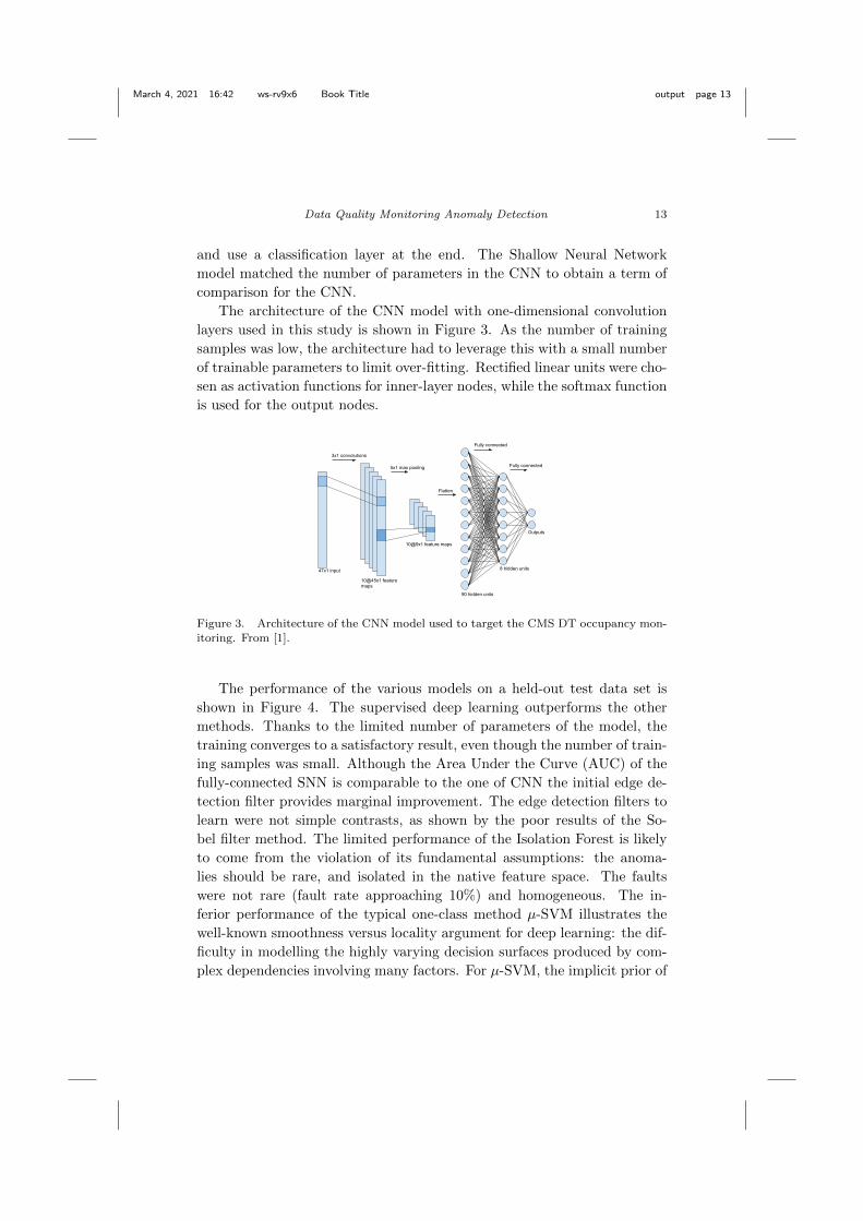
The architecture of the CNN model with one-dimensional convolution

layers used in this study is shown in Figure 3. As the number of training

samples was low, the architecture had to leverage this with a small number

of trainable parameters to limit over-fitting. Rectified linear units were cho-

sen as activation functions for inner-layer nodes, while the softmax function

is used for the output nodes.

Outputs

8 hidden units

90 hidden units

10@9x1 feature maps

10@45x1 feature maps

47x1 input

3x1 convolutions

5x1 max pooling

Flatten

Fully connected

Fully connected

Figure 3. Architecture of the CNN model used to target the CMS DT occupancy mon-

itoring. From [1].

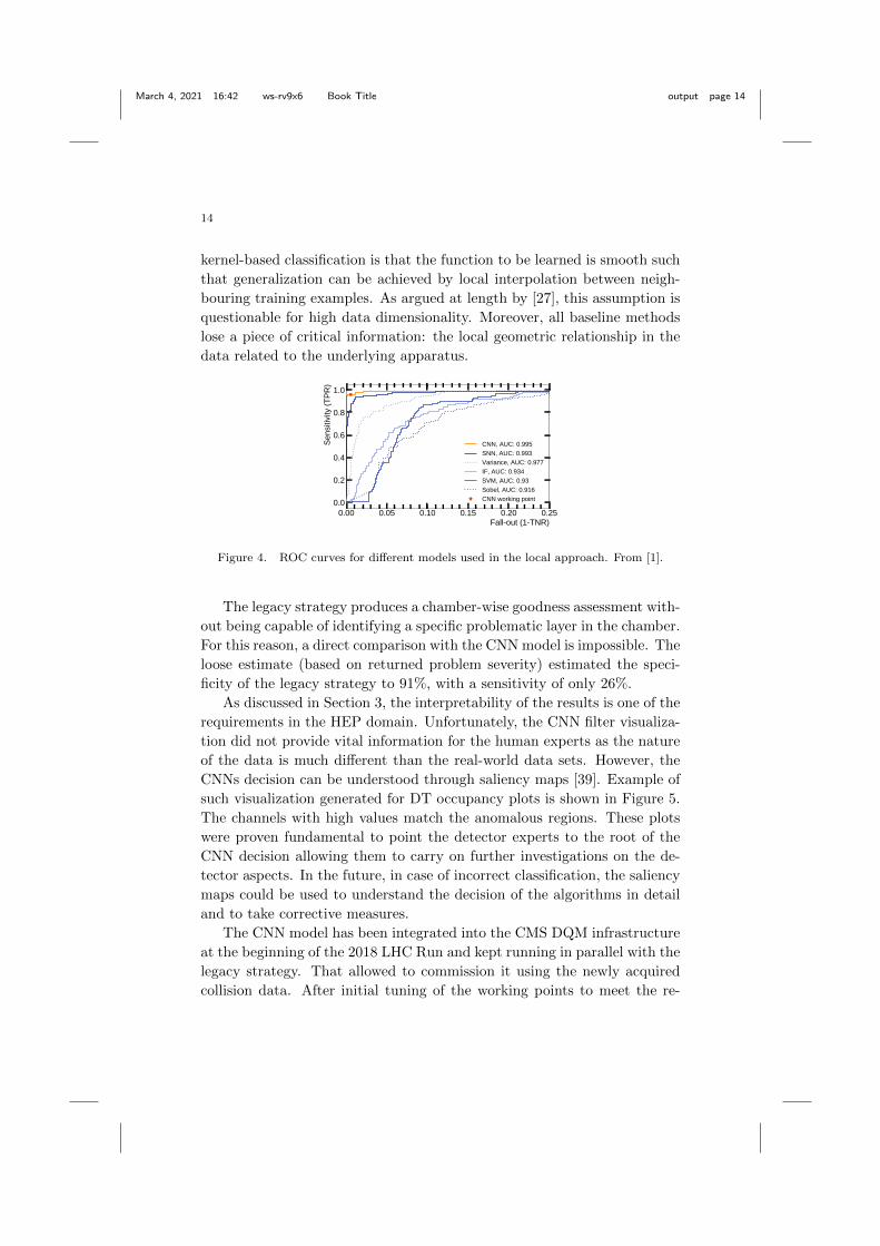
The performance of the various models on a held-out test data set is

shown in Figure 4. The supervised deep learning outperforms the other

methods. Thanks to the limited number of parameters of the model, the

training converges to a satisfactory result, even though the number of train-

ing samples was small. Although the Area Under the Curve (AUC) of the

fully-connected SNN is comparable to the one of CNN the initial edge de-

tection filter provides marginal improvement. The edge detection filters to

learn were not simple contrasts, as shown by the poor results of the So-

bel filter method. The limited performance of the Isolation Forest is likely

to come from the violation of its fundamental assumptions: the anoma-

lies should be rare, and isolated in the native feature space. The faults

were not rare (fault rate approaching 10%) and homogeneous. The in-

ferior performance of the typical one-class method µ-SVM illustrates the

well-known smoothness versus locality argument for deep learning: the dif-

ficulty in modelling the highly varying decision surfaces produced by com-

plex dependencies involving many factors. For µ-SVM, the implicit prior of


14

kernel-based classification is that the function to be learned is smooth such

that generalization can be achieved by local interpolation between neigh-

bouring training examples. As argued at length by [27], this assumption is

questionable for high data dimensionality. Moreover, all baseline methods

lose a piece of critical information: the local geometric relationship in the

data related to the underlying apparatus.

0.00 0.05 0.10 0.15 0.20 0.25Fallout 1TNR)

0.0

0.2

0.4

0.6

0.8

1.0

Sen

)itivit. TPR)

CNN, AUC: 0.995SNN, AUC: 0.993Variance, AUC: 0.977IF, AUC: 0.934SVM, AUC: 0.93Sobel, AUC: 0.916CNN working point

Figure 4. ROC curves for different models used in the local approach. From [1].

The legacy strategy produces a chamber-wise goodness assessment with-

out being capable of identifying a specific problematic layer in the chamber.

For this reason, a direct comparison with the CNN model is impossible. The

loose estimate (based on returned problem severity) estimated the speci-

ficity of the legacy strategy to 91%, with a sensitivity of only 26%.

As discussed in Section 3, the interpretability of the results is one of the

requirements in the HEP domain. Unfortunately, the CNN filter visualiza-

tion did not provide vital information for the human experts as the nature

of the data is much different than the real-world data sets. However, the

CNNs decision can be understood through saliency maps [39]. Example of

such visualization generated for DT occupancy plots is shown in Figure 5.

The channels with high values match the anomalous regions. These plots

were proven fundamental to point the detector experts to the root of the

CNN decision allowing them to carry on further investigations on the de-

tector aspects. In the future, in case of incorrect classification, the saliency

maps could be used to understand the decision of the algorithms in detail

and to take corrective measures.

The CNN model has been integrated into the CMS DQM infrastructure

at the beginning of the 2018 LHC Run and kept running in parallel with the

legacy strategy. That allowed to commission it using the newly acquired

collision data. After initial tuning of the working points to meet the re-



A

0 10 20 30 40 50 60Channel

159

Laye

r

a.u.

CMS Saliency Map, Run: 272011, W: 1.0, St: 1.0, Sec: 6.0

0.00

5.00

B

0 10 20 30 40 50 60Channel

159

Laye

r

a.u.


0.00

5.00

C

0 10 20 30 40 50 60Channel

159

Laye

r

a.u.


0.00

5.00

Figure 5. Example of visualization of saliency maps for three CMS DT chambers cor-

responding to input occupancy plots from Figure 1. The scale is proportional to thechannel influence over classifier decision to flag problems. From [8].

quirements of the DT detector experts, the algorithm has been performing

reliably, and it is considered for deployment in the next LHC Run.

4.2. One-class Anomaly Detection

In normal conditions, the healthy DT chambers show similar occupancy

levels in adjacent layers with the four inner layers having a different be-

haviour due to their different spatial orientation. The convolutional au-

toencoder used in [1] exploited the patterns of relative occupancy of the

layers within a chamber. This approach extended and complemented the

one presented in the previous Section 4.1, allowing to identify less frequent

intra-chamber problems which require the comparison of the information

about all layers within one chamber to be spotted. Typical examples of

these kinds of failures are problems related to the high-voltage bias. The

voltage distribution system is organized by layers and a lower value w.r.t to


16

the nominal operation point would result in lower detector efficiency and,

as a consequence, lower absolute occupancy in the affected region.

In this study, the dataset was cleaned from the common anomalies using

the CNN model from Section 4.1 to save time on manual labelling and ac-

quire sizeable dataset. Then the autoencoder-based model was trained to

properly reconstruct healthy behaviour. Finally, the autoencoder-based

model was tested on a set of occupancy plots where chambers showed

problems in a particular layer (layer 9). Figure 6 shows that the mean

squared reconstruction error (MSE) integrated over healthy regions (even

from anomalous chambers) is lower than the one from anomalous ones. Of

course, the severity of the problem matters and layers operating in 3450 V

are more difficult to be detected than the ones operating in 3200 V. To

summarize, the detector experts can design custom metrics, integrating

the MSE over the areas of interest to further extend the monitoring infras-

tructure.

0.00 0.05 0.10 0.15 0.20 0.25 0.30Layer 3 MSE

0

100

101

102

Cha

mbe

rs Layer 9 at 3200VLayer 9 at 3450VLayer 9 at nominal

0.0 0.1 0.2 0.3 0.4 0.5 0.6 0.7Layer 9 MSE

0

100

101

102

Cha

mbe

rs Layer 9 at 3200VLayer 9 at 3450VLayer 9 at nominal

Figure 6. MSE between reconstructed and input samples for layer 3 (left) and layer 9(right) for three categories of data. Despite a problem in layer 9, all MSEs for layer 3

are comparable for all chambers. The nominal voltage falls between 3550 and 3600 V.

From [1].

4.3. Unsupervised Anomaly Detection

Finally, [1] showed that a byproduct of the undercomplete autoencoders, i.e

the lower dimensional latent representation, can be further plotted to visu-

ally track novel behaviour patterns and emerging problems. For instance

the DT chambers 3-dimensional latent representation clusters according

to the chamber position in the CMS detector, shown in Figure 7. When

the chamber behaviour changes, so will the manifold. Higher dimension

manifods can be used as well, e.g. to perform classification.



Dimension 1

−30 −20 −100

Dimension 2

−60−40

−200

Dimen

sion

3

−20

−10

0

Station 1

Station 2

Station 3

Figure 7. Compressed representations of chamber level data for all chambers in thedataset. The representations are clustering (right) according to their positions in the

detector, i.e. station number. The DT numbering schema is shown on the left. From [1].

5. Data Certification Novelty Detection with Deep Autoen-

coders

This section presents an approach of applying autoencoders to automate

the DQM scrutiny, with the example of the CMS data certification process

(Section 2.4) and results from [2]. With a tolerance for false negatives, the

autoencoders will reduce the manual work as discussed in [40]. [2] used data

for the physics certification process (see Section 2.4). The data set used in

this work consisted of 163684 LSs recorded from June to October 2016. In

total, 401 physics variables were used (e.g. transverse momentum, energy,

multiplicity, direction for the different physics objects). The binary quality

labels determined by the manual certification procedure performed by the

detector experts were used for evaluating model’s performance.

The human experts make decisions regarding the data quality based on

the shape of the statistical distributions of key quantities represented in

the form of histograms. In the case of an anomaly, the corresponding his-

tograms should show a considerable deviation from the nominal shape (for

visual interpretation see Figure 8). To mimic this logic, the distribution

Di = {x0, . . . , xk} of each one of the 401 used variables was represented by

its summary statistics using five quantiles, mean and standard deviation.

The final vector has 2807 features. Each data-point represents the data

acquired during one LS to aim for high time granularity of the classifica-

tion results. The high dimensionality and non-linear dependencies between

variables preclude the use of traditional anomaly detection techniques. In-


18

stead, different autoencoder regularization techniques were examined. The

final Receiver Operating Characteristic (ROC) curves of autoencoders and

their corresponding AUC are shown in Figure 9.

Figure 8. Two examples of histograms related to the CMS Pixel detector status for a

normal (left) and anomalous (right) LS. The reference shape is the Landau distribution.

The bad LS manifests anomaly in low charge, which is caused by the Pixel detectornot being properly synchronized with the bunch crossing. Such distributions, obtained

for each LS, are preprocessed into a summary statistics vector of seven variables: five

quantiles, mean and standard deviation. From [8].

0.0 0.2 0.4 0.6 0.8 1.0False Positive Rate

0.5

0.6

0.7

0.8

0.9

1.0

True Positive Rate

Undercomplete Autoencoder, AUC = 0.895 ± 0.004Contractive Autoencoder, AUC = 0.895 ± 0.003Variational Autoencoder, AUC = 0.901 ± 0.003Sparse Autoencoder, AUC = 0.905 ± 0.003

Figure 9. ROC and AUC of the autoencoder models using different regularization tech-

niques. The bands correspond to variance computed after running the experiment five

times using random weight initialization. From [2].

Beyond performance, a valuable model for the certification task needs

to provide easily interpretable results allowing the experts to pinpoint the

root of a problem. In this respect, the autoencoder approach provides a

clear advantage allowing to evaluate the contribution to the MSE metric of

each input variable. Misbehaving variables can be easily singled out based

on their high contribution to the overall error. Figure 10 illustrates one



example of how this can be exploited on the CMS data. The features are

grouped according to their sensitivity to a particular physics property. The

plot of the absolute error allows the expert to identify the problematic area

at a glance judging on the absolute size of the error for the variable or group

of variables.

pf_jets

cal_jet_mets

pho

muons

pf_jets2

pf_m

ets

nvtx

cal_jet_mets2sc cc

pho2

muons2

ebs

hbhef

presh

0

2

4

6

8

10

Abs

olute Error

pf_jets

cal_jet_mets

pho

muons

pf_jets2

pf_m

ets

nvtx

cal_jet_mets2sc cc

pho2

muons2

ebs

hbhef

presh

0

200

400

600

800

1000

Abs

olute Error

Figure 10. Reconstruction error of each feature for two samples. Different colours

represent features linked to different physics objects. For a negative sample (left) similarautoencoder reconstruction errors are expected across all objects with small absolute

scale. Anomalous samples (right) have visible peaks for problematic features (muons).

From [2].

6. Trigger Rate Anomaly Detection with Conditional Vari-

ational Autoencoders

[41] targets improving anomaly detection for the trigger system (Sec-

tion 2.3) with VAEs. To avoid the pitfalls described in Section 3, the

key is to exploit the hierarchical structure of the trigger system to input

all available observation into the VAE, to constrain the representation, by

separating the known factors from the other unknown sources or variabil-

ity. The model, called AD-CVAE, includes the architecture, as a specific

realization of conditional variational autoencoders (CVAE) [42–44], as well

as the corresponding loss function and a detection metrics. Overall, the

contribution shows that a regular CVAE architecture can be exploited for

general anomaly detection tasks in HEP context. More details and experi-

ments are available in [41].


20

6.1. Problem statement

The current CMS trigger monitoring system is based on the comparison be-

tween the observed per-node rate and its reference value for the measured

PU value. While the current implementation is quite effective in spotting

erratic changes for a single node, it is less sensitive to collective changes on

several nodes that could equally affect the overall acceptance rate. In par-

ticular, about 600 nodes of the HLT can be grouped in several configuration

groups, showing strong correlations in their acceptance rate variations, see

Figure 11.

0 100 200 300 400Trigger ID

0

100

200

300

400

Trig

ger ID

−1.00

−0.75

−0.50

−0.25

0.00

0.25

0.50

0.75

1.00

Figure 11. Correlations between 458 HLT rates of fill 6291 of LHC Run 2. From [8].

The dominant cause of correlation is structural, known and measur-

able: the direct, pre-configured link from a set of L1 nodes to an HLT node

through a specific configuration (Figure 12). However, more subtle and

un-reported causes can create correlations: physics processes when differ-

ent nodes select the same physics objects with different requirements (e.g.

different requests on its energy); or utilization of the same sub-detector

component or software component across different nodes. The correspond-

ing graphical structure must include these unknowns.

To correctly model the trigger system, the algorithm has to successfully

disentangle the dependence of HLT rates on L1 rates from all other unknown



HLT HLT HLT HLT HLT HLT HLT HLT HLT HLT HLT

L1 L1 L1 L1 L1 L1 L1 L1 L1 L1

Figure 12. Simplified, schematic graph inspired by the trigger system configuration.

Blue nodes represent HLT while yellow L1. Each link is unidirectional starting fromyellow nodes. For each LHC fill the graph has a few hundred nodes. The connection

between L1 and HLT nodes can be seen as a hierarchical directed graph from the L1 tothe HLT system. From [41].

processes. In light of the results of [45], the disentanglement objective in

generative models cannot be met by fully unsupervised VAE architectures.

The alternative is to enforce disentanglement through a structured condi-

tional architecture.

The second issue is: what are the anomalies, and the normal behavior?

We are interested in highlighting instances where we observe:

• big change on a single feature called Type A anomaly (to repro-

duce the functionality of the current monitoring), or

• small but systematic change in a structural configuration group,

called Type B anomaly (novel strategy).

On the contrary, an instance x with a problem of small severity and on

a group of uncorrelated features should be considered as an inlier, corre-

sponding to expected statistical fluctuations.

While dealing with Type A anomalies is relatively well managed, the

CMS experiment currently does not provide any tools to track problems

falling into the Type B category.

6.2. The architecture

The goal of the architecture is to address the disentanglement issue, in other

words to build a representation within the VAE framework where the known

and unknowns factors are identified. This includes both the structure of the

representation, and a loss function that takes into account the conditioning

on the known factors. The formal model is a follows: the observable x is a

function of k (known) and u (unknown) latent vectors, i.e; x = f(k;u). k

and u are assumed to be marginally independent. In the trigger context, x

is the feature vector of observed HLT rates [x1, x2, ..., xn], k is the vector


22

of observed L1 rates, and u stands for the unknown factors. Conceptually,

features associated with the same subset of the k vector correspond to a

structural configuration group. The variable u allows for modelling multiple

modes in the conditional distribution p(x|k) making the model sufficient for

modelling one-to-many mapping.

This defines the conditional directed graphical model of Figure 13, where

the input observations modulate the prior on latent variables to model

the distribution of high-dimensional output space as a generative model

conditioned on the input observation. The conditional likelihood func-

tion pθ(x|u, k) is formed by a non-linear transformation, with parameters

θ. φ is another non-linear function that approximates inference posterior

qφ(u|k, x) = N(µ, σI).

ku

xφ

θ

Figure 13. An example of CVAE as a directed graph. Solid lines denote the generative

model pθ(x|u, k)pθ(u). Dashed lines denote variational approximation qφ(u|x, k). Both

variational parameters θ and generative parameters φ are learned jointly. From [41].

The φ and θ functions are implemented as deep neural networks with

non-linear activation functions. Figure 14 shows the autoencoder architec-

ture corresponding to Figure 13 as a block diagram.

This model, called AD-CVAE, is trained efficiently in the framework of

stochastic gradient variational Bayes. The usual loss function of VAE is

the so-called Evidence Lower Bound, which is a tractable proxy for opti-

mizing the log-likelihood of the data. With the conditioning on k taken

into account, the modified objective lower bound is:

log pθ(x) ≥ Eqφ(z|k,x)[log pθ(x|z)pθ(x|k)]− DKL(qφ(z|x, k)||p(z)) , (1)

where z (Gaussian latent variable) intends to capture non-observable factors

of variation u.

6.3. The loss function

The original works on VAEs by [29, 30] proposed a full (diagonal) Gaussian

observation model, that is

Pθ(x|z) = N (µ, σI),



μ

σ

z

k

ENCODERDECODER

μ1

σ1

μ2

σ2

μj

σj

…

x

Figure 14. Architecture of CVAE targeting trigger system anomaly detection. Observ-able data x depends on z (capturing non-observable factors of variation u) and k vectors.

From [8].

where both the multidimensional mean vector and the multidimensional

variance vector are to be learnt. However, in most practical applications

the VAE evaluates the reconstruction loss with a simple mean squared error

(MSE) between the data x and the output of the decoder. Such an approach

suffers from a very serious issue. It is equivalent to setting the observation

model pθ(x|z) as a normal distribution of fixed variance σ = 1.

Fixing the variance this way can be detrimental to learning as it puts a

limit on the accessible resolution for the decoder. Instead, the model can

learn the variance of the output of the decoder feature-wise (i running as

the dimensionality of the data vectors x):

− log pθ(x|z) =∑i

(xi − µi)2

2σ2i

+ log(√

2πσi

). (2)

Learning the reconstruction variance allows the model to find the op-

timal reconstruction resolution for each feature of the data, separating the

intrinsic noise from the actual data structure. Although it has been argued

that this approach can challenge the optimization process [33, 46], there

were no reported challenges when training the AD-CVAE.

After inserting equation 2 as the reconstruction objective to the general

loss defined in equation 1 the final objective of AD-CVAE is:

LAD-CVAE(x, k, θ, φ) =∑i

(xi − µi)2

2σ2i

+log(√

2πσi

)+DKL(qφ(z|x, k)||p(z)).

(3)

6.4. Anomaly metrics

Once the model parameters are learned, one can detect anomalies:

• of type A with average infinity norm of the reconstruction loss

mA = || 1σ (x− x)2||∞, where x is the reconstructed mean and σ is

the reconstructed variance of decoder output;


24

• of type B with KL divergence mB = DKL(qφ(z|x, k)||p(z)), known

as information gain.

In the first case, an anomaly is identified on a single feature. For a given

data point (x, k), the evaluation of the loss of the VAE at this data point

L(x, k) is an upper-bound approximation of − log pθ(x|k), measuring how

unlikely the observation x is to the model given k. AD-CVAE thus provides

here a model that naturally estimates how anomalous x is given k, rather

than how anomalous the couple (x, k) is. That means that a rare value of

k associated with a proper value for x should be treated as non-anomalous,

which is the goal. The binary indicator is obtained by thresholding the

value, a typical strategy for anomaly detection. With thresholding, the

choice of the infinity norm of the reconstruction error instead of the mean is

required. A mean of the reconstruction error would be uninformative when

most of the features do not manifest abnormalities and, as a consequence,

lower overall anomaly score.

As argued in [47], the DKL measures the amount of additional infor-

mation needed to represent the posterior distribution given the prior over

the latent variable being explored to explain the current observation. The

lower the absolute value of DKL, the more predictable state is observed.

The DKL was then used as a surprise quantifier, e.g. in [47, 48] when the

model was exposed to held-out images. [35, 36] explored DKL as an indicator

of out of distribution samples. For type B outliers, the expected anomaly

systematically reinforces patterns in data. It is then expected that not cal-

ibrated model allocates such information using the latent bits, allowing for

a successful reconstruction. On the other hand, changes in uncorrelated

features will be removed in the encoding process, resulting in low recon-

struction likelihood. Hence anomalous input yields higher values of mB

and likelihood at the same time. Thus, mB must be detached from the

reconstruction part of the loss function as combining metrics is detrimental

to the detection results.

Because of two separate failure scenarios, the metrics are not combined

in one overall score but rather use logical OR to determine anomalous in-

stances.

6.5. Experimental results

CVAE model was evaluated on two datasets: a synthetic one and on the

real trigger dataset. The synthetic data set is a version of the Gaussian

Mixture Model and was implemented as an initial benchmark that proxies



the trigger data set. For testing, the samples are generated according to

the table:

Test set Description

Type A Inlier Generated in the same process as training data

Type A Anomaly 5σ change on ε for a random feature

Type B Inlier 3σ change on ε for a random set of correlated features

Type B Anomaly 3σ change on ε for a random feature cluster

The choice of 5σ and 3σ comes from the legacy requirements of our target

application. The real HLT rates are treated as x and L1 Trigger rates as k.

The proposed prototype used 4 L1 Trigger paths that seeded 6 unique HLT

paths each. The dataset totalled 102895 samples from which 2800 samples

were used for testing. Again the hypothetical situations that are likely to

happen in the production environment were considered. Four synthetic test

datasets were generated manipulating the test set similarly to the synthetic

dataset (based on the table above).

The results are reported in Figure 15. Given the high order of the

deviation on Type A anomalies, the model easily spots them. Also, Type

B detection results show that CVAE is outperforming VAE baseline and

confirming it is suitable for a task in question. The performance of the

algorithm on CMS dataset is matching the performance we reported for

the synthetic one.

0.0 0.2 0.4 0.6 0.8 1.0Fallout 1TNR)

0.0

0.2

0.4

0.6

0.8

1.0

Sen

sitivity TPR)

CVAE:TypeA,||1σ (x− x2||∞,AUC=0.996±0.002CVAE:TypeB,μ(ⅅμL),AUC=0.826±0.010VAE:TypeB,μ(ⅅμL),AUC=0.686±0.027

0.0 0.2 0.4 0.6 0.8 1.0Fallout 1TNR)

0.0

0.2

0.4

0.6

0.8

1.0

Sen

siti(

it)

TP

R)

CVAE:T)peA,||1σ (x− x2||∞,AUC=0.984±0.008

CVAE:T)peB,μ(ⅅμL),AUC=0.826±0.039VAE:T)peB,μ(ⅅμL),AUC=0.675±0.008

Figure 15. The ROC curves for two anomaly detection problems using synthetic (left)and CMS trigger rates test dataset (right). The bands correspond to σ computed after

running the experiment 5 times. From [41].


26

7. LHC Monitoring with LSTMs

Recurrent models can be applied to temporal or sequential data, where the

order of data is important. Recurrent Neural Networks (RNNs) [49] can

process sequential data element-by-element. In this way, they can model

sequential and time dependencies on multiple scales. However, the influence

of a given input on hidden and output layers during the training often

results in gradient either decaying or exponentially grow as it moves across

recurrent connections. This effect is described as the vanishing or exploding

gradient problem. A successful attempt to prevent this phenomenon is the

Long-Short Term Memory (LSTM) network [50], through the introduction

of internal state node and forget gate.

In this section, we summarize the results of the experiments from [51].

The authors validated the performance of the LSTM network in a voltage

time series modelling task, see the description of the problem in Section 2.5.

The data used in the experiments consisted of many years of magnet

activity. A group of 600 A magnets, that generated the highest number

of quench events, were used. The anomalous events were not only sparse

but also challenging to find, as the logging database does not enable au-

tomated quench periods extraction. The authors developed an extraction

application, automating the dataset generation. In the experiments, dif-

ferent lengths of time window frame were considered. Finally, the 24 h

window ahead of a quench event were chosen, totalling 425 from the period

of 2008 and 2016.

Figure 16. The LSTM-based neural network used for the experiments in [51].

The LSTM model yielding the best results is shown in Figure 16. The



tests considered the ability of a model to anticipate forward voltage values.

Figure 17 shows the predicted voltage readings. The authors used Root

Mean Square Error (RMSE) and Mean Percentage Error (MPE) to assess

the algorithm performance. The RMSE results are presented in Figure 18,

where L corresponds to the number of previous time steps as input and

B corresponds to a training batch size. The best results were obtained

with L = 16 and B = 2048. After verifying that the model can predict

forward voltage readings, the ultimate challenge was to select a threshold

of RMSE value determining which readings should be considered anoma-

lous. Unfortunately, this value has not been chosen and requires further

investigation.

Figure 17. The LSTM-based neural network voltage predictions for one step ahead

(left) and two steps ahead (right). From [51].

Figure 18. The value of RMSE as a function of prediction steps for different batch size

B and the number of previous time steps L values with 32 neurons in the middle LSTMlayer. From [51]

The resulting model promises to speed up the quench detection and pre-

vention process. Besides the model, the authors developed a visualization

framework and tested the model on FPGAs, as the system reaction time is

critical.


28

8. Conclusion

In this chapter, we discussed novel approaches to improve the accuracy of

Data Quality applications for High Energy Physics experiments. Taking as

an example the CMS experiment at the Large Hadron Collider, we showed

how anomaly detection techniques based on Machine Learning algorithms

could detect unforeseen detector malfunctioning. We also showed how the

flexibility of Deep Learning architecture allows one to enforce known causal

relation between data, through constraints built by connections in the net-

work architecture. The results demonstrate that the techniques based on

DNNs provide a breakthrough for complex and high dimensional problems

in infrastructure monitoring. The results show remarkable efficiency on

currently tracked failure modes, extend current monitoring coverage and

provide ways to interpret the results. These aspects are of paramount im-

portance in a system which will need to be operated for years by field

experts.

While the discussion was limited to specific datasets related to the CMS

experiment, the applications are of general interest for High Energy Physics

experiments. Some of the proposed methods have already been integrated

and deployed in the CMS DQM infrastructure. A generalization of these

strategies could pave the way to full automation of the quality assessment

for HEP experiments and accelerator complexes.

References

[1] A. A. Pol, G. Cerminara, C. Germain, M. Pierini, and A. Seth, Detectormonitoring with artificial neural networks at the cms experiment at thecern large hadron collider, Computing and Software for Big Science 3(2019) 1, 3.

[2] A. A. Pol, V. Azzolini, G. Cerminara, F. De Guio, G. Franzoni, M. Pierini,F. Siroky, and J.-R. Vlimant, Anomaly detection using deep autoencodersfor the assessment of the quality of the data acquired by the cmsexperiment, in EPJ Web of Conferences, EDP Sciences. 2019.

[3] D. Abbott, G. Aad, B. Abbott, L. Ambroz, G. Artoni, M. Backes, J. Frost,A. Cooper-Sarkar, G. Gallardo, T. Huffman, et al., Atlas data qualityoperations and performance for 2015–2018 data-taking, Journal ofInstrumentation 15 (2020) 04, .

[4] M. Adinolfi, D. Derkach, F. Archilli, A. Baranov, A. Panin, A. Pearce,A. Ustyuzhanin, and W. Baldini, Lhcb data quality monitoring, in J. Phys.Conf. Ser. 2017.

[5] B. von Haller, F. Roukoutakis, S. Chapeland, V. Altini, F. Carena,W. Carena, V. C. Barroso, F. Costa, R. Divia, U. Fuchs, et al., The alice



data quality monitoring, in Jfournal of Physics: Conference Series, IOPPublishing. 2010.

[6] M. Schneider, The Data Quality Monitoring software for the CMSexperiment at the LHC: past, present and future, in Proceedings to CHEP2018. 2018.

[7] CMS, V. Khachatryan et al., The CMS trigger system, JINST 12 (2017)01, P01020, arXiv:1609.02366 [physics.ins-det].

[8] A. A. Pol, Machine Learning Anomaly Detection Applications to CompactMuon Solenoid Data Quality Monitoring. PhD thesis, UniversiteParis-Saclay, 2020.

[9] C. Roderick, G. Kruk, and L. Burdzanowski, The cern accelerator loggingservice-10 years in operation: a look at the past, present and future, tech.rep., CERN, 2013.

[10] L. Bottura, Cable stability, arXiv preprint arXiv:1412.5373 (2014) .[11] R. Denz, Electronic systems for the protection of superconducting elements

in the lhc, IEEE transactions on applied superconductivity 16 (2006) 2,1725.

[12] J. Steckert and A. Skoczen, Design of fpga-based radiation tolerant quenchdetectors for lhc, Journal of Instrumentation 12 (2017) 04, T04005.

[13] D. M. Blei, A. Kucukelbir, and J. D. McAuliffe, Variational Inference: AReview for Statisticians, Journal of the American Statistical Association112 (2017) 518, 859. https://arxiv.org/abs/1601.00670.

[14] C. C. Aggarwal, Outlier Analysis. Springer Publishing Company,Incorporated, 2nd ed., 2016.

[15] R. Chalapathy and S. Chawla, Deep learning for anomaly detection: Asurvey, arXiv preprint arXiv:1901.03407 (2019) .

[16] M. Goldstein and S. Uchida, A comparative evaluation of unsupervisedanomaly detection algorithms for multivariate data, PloS one 11 (2016) 4,e0152173.

[17] A. Zimek, E. Schubert, and H.-P. Kriegel, A survey on unsupervised outlierdetection in high-dimensional numerical data, Statistical Analysis andData Mining: The ASA Data Science Journal 5 (2012) 5, 363.

[18] C. C. Aggarwal, A. Hinneburg, and D. A. Keim, On the SurprisingBehavior of Distance Metrics in High Dimensional Spaces, in Proceedingsof the 8th International Conference on Database Theory, ICDT ’01.Springer-Verlag, Berlin, Heidelberg, 2001.

[19] A. Hinneburg, C. C. Aggarwal, and D. A. Keim, What is the nearestneighbor in high dimensional spaces?, in 26th Internat. Conference on VeryLarge Databases. 2000.

[20] Y. LeCun, Y. Bengio, et al., Convolutional networks for images, speech,and time series, The handbook of brain theory and neural networks 3361(1995) 10, 1995.

[21] B. Scholkopf, J. C. Platt, J. Shawe-Taylor, A. J. Smola, and R. C.Williamson, Estimating the support of a high-dimensional distribution,Neural computation 13 (2001) 7, 1443.

[22] F. T. Liu, K. M. Ting, and Z.-H. Zhou, Isolation forest, in Data Mining,


30

2008. ICDM’08. Eighth IEEE International Conference on, IEEE. 2008.[23] F. T. Liu, K. M. Ting, and Z.-H. Zhou, Isolation-based anomaly detection,

ACM Transactions on Knowledge Discovery from Data (TKDD) 6 (2012)1, 3.

[24] R. Shwartz-Ziv and N. Tishby, Opening the black box of deep neuralnetworks via information, CoRR abs/1703.00810 (2017) .

[25] D. Hendrycks and K. Gimpel, A baseline for detecting misclassified andout-of-distribution examples in neural networks, arXiv preprintarXiv:1610.02136 (2016) .

[26] G. E. Hinton, Connectionist learning procedures, in Machine learning,pp. 555–610. Elsevier, 1990.

[27] Y. Bengio, A. Courville, and P. Vincent, Representation Learning: AReview and New Perspectives, IEEE Trans. Pattern Anal. Mach. Intell. 35(Aug., 2013) 1798. https://doi.org/10.1109/TPAMI.2013.50.

[28] G. Alain and Y. Bengio, What regularized auto-encoders learn from thedata-generating distribution, The Journal of Machine Learning Research 15(2014) 1, 3563.

[29] D. P. Kingma and M. Welling, Auto-encoding variational bayes, arXivpreprint arXiv:1312.6114 (2013) .

[30] D. J. Rezende, Stochastic Backpropagation and Approximate Inference inDeep Generative Models, in Proceedings of the 31st InternationalConference on International Conference on Machine Learning - Volume 32,ICML. 2014.

[31] J. An and S. Cho, Variational Autoencoder based Anomaly Detection usingReconstruction Probability, tech. rep., SNU Data Mining Center, 2015.

[32] X. Wang, Y. Du, S. Lin, P. Cui, and Y. Yang, Self-adversarial variationalautoencoder with gaussian anomaly prior distribution for anomalydetection, CoRR abs/1903.00904 (2019) , arXiv:1903.00904.http://arxiv.org/abs/1903.00904.

[33] S. Zhao, J. Song, and S. Ermon, Infovae: Information maximizingvariational autoencoders, CoRR abs/1706.02262 (2017) .http://arxiv.org/abs/1706.02262.

[34] D. J. Rezende and F. Viola, Taming vaes, arXiv preprint arXiv:1810.00597(2018) .

[35] E. Nalisnick, A. Matsukawa, Y. W. Teh, and B. Lakshminarayanan,Detecting out-of-distribution inputs to deep generative models using a testfor typicality, arXiv preprint arXiv:1906.02994 (2019) .

[36] J. Snoek, Y. Ovadia, E. Fertig, B. Lakshminarayanan, S. Nowozin,D. Sculley, J. Dillon, J. Ren, and Z. Nado, Can you trust your model’suncertainty? evaluating predictive uncertainty under dataset shift, inAdvances in Neural Information Processing Systems. 2019.

[37] Y. Kawachi, Y. Koizumi, and N. Harada, Complementary set variationalautoencoder for supervised anomaly detection, in IEEE InternationalConference on Acoustics, Speech and Signal Processing (ICASSP). 2018.

[38] D. Hendrycks, M. Mazeika, and T. G. Dietterich, Deep anomaly detectionwith outlier exposure, CoRR abs/1812.04606 (2018) , arXiv:1812.04606.



http://arxiv.org/abs/1812.04606. ICLR19.[39] K. Simonyan, A. Vedaldi, and A. Zisserman, Deep inside convolutional

networks: Visualising image classification models and saliency maps, arXivpreprint arXiv:1312.6034 (2013) .

[40] M. Borisyak, F. Ratnikov, D. Derkach, and A. Ustyuzhanin, Towardsautomation of data quality system for cern cms experiment, arXiv preprintarXiv:1709.08607 (2017) .

[41] A. Pol, V. Berger, G. Cerminara, C. Germain, and M. Pierini, Trigger rateanomaly detection with conditional variational autoencoders at the cmsexperiment, in Machine Learning and the Physical Sciences Workshop atthe 33rd Conference on Neural Information Processing Systems (NeurIPS).2019.

[42] D. P. Kingma, S. Mohamed, D. J. Rezende, and M. Welling,Semi-supervised learning with deep generative models, in Advances inneural information processing systems. 2014.

[43] K. Sohn, H. Lee, and X. Yan, Learning structured output representationusing deep conditional generative models, in Advances in neuralinformation processing systems. 2015.

[44] M. F. Mathieu, J. J. Zhao, J. Zhao, A. Ramesh, P. Sprechmann, andY. LeCun, Disentangling factors of variation in deep representation usingadversarial training, in Advances in Neural Information Processing Systems29, D. D. Lee, M. Sugiyama, U. V. Luxburg, I. Guyon, and R. Garnett,eds., pp. 5040–5048. Curran Associates, Inc., 2016.

[45] F. Locatello, S. Bauer, M. Lucic, G. Raetsch, S. Gelly, B. Scholkopf, andO. Bachem, Challenging common assumptions in the unsupervised learningof disentangled representations, in Proceedings of the 36th InternationalConference on Machine Learning, K. Chaudhuri and R. Salakhutdinov,eds. PMLR, Long Beach, California, USA, 09–15 Jun, 2019.http://proceedings.mlr.press/v97/locatello19a.html.

[46] J. Lucas, G. Tucker, R. Grosse, and M. Norouzi, Understanding posteriorcollapse in generative latent variable models, .

[47] M. Gemici, C.-C. Hung, A. Santoro, G. Wayne, S. Mohamed, D. J.Rezende, D. Amos, and T. Lillicrap, Generative temporal models withmemory, arXiv preprint arXiv:1702.04649 (2017) .

[48] S. A. Eslami, D. J. Rezende, F. Besse, F. Viola, A. S. Morcos, M. Garnelo,A. Ruderman, A. A. Rusu, I. Danihelka, K. Gregor, et al., Neural scenerepresentation and rendering, Science 360 (2018) 6394, 1204.

[49] K. Kawakami, Supervised sequence labelling with recurrent neural networks,Ph. D. dissertation, PhD thesis. Ph. D. thesis (2008) .

[50] S. Hochreiter and J. Schmidhuber, Long short-term memory, Neuralcomputation 9 (1997) 8, 1735.

[51] M. Wielgosz, A. Skoczen, and M. Mertik, Using lstm recurrent neuralnetworks for monitoring the lhc superconducting magnets, NuclearInstruments and Methods in Physics Research Section A: Accelerators,Spectrometers, Detectors and Associated Equipment 867 (2017) 40.

Documents

Data Quality Monitoring Anomaly Detection