Embed Size (px)
Citation preview
Data Rate Performance Gains in UMTS Evolution to LTE
at the Cellular Level
Pedro Atanásio Carreira
Dissertation submitted for obtaining the degree of
Master in Electrical and Computer Engineering
Jury
Supervisor: Prof. Luís M. Correia
Co-Supervisor: Eng. Ricardo Dinis
President: Prof. José Bioucas Dias
Member: Prof. António Rodrigues
October 2011

ii

iii
To the Ones I love

iv

v
Acknowledgements
Acknowledgements
First of all, I would like to thank Professor Luís Correia, for giving me the opportunity to work on this
thesis. His discipline and supervision are reflected on the final work presented. Furthermore, the
expertise felt within GROW and the interesting works presented within the group gave rise to what I
found to be a compelling environment to learn and develop a critical attitude about research topics
presented. Also, the partnership established with a national telecom operator allowed for additional
motivation and interest in the development of the work.
To Optimus, namely Eng. Luís Santo, Eng. Ricardo Dinis and Eng. Sérgio Gonçalves, for their initial
work planning and for their friendly and always available attitude, despite their limited time. Being able
to conduct measurements in a live LTE cluster brings great added value to the work performed, and
the technical support provided throughout thesis development largely contributed to the work success.
To the Professors who have contributed for my personal development, namely Prof. Ana Fred, who
allowed me to learn on such interesting topics as data clustering, Prof. António Rodrigues and João
Sobrinho, for their always available and friendly attitude, intrinsically combined with good teaching.
Also to Prof. Rui Castro for the friendly attitude and for the great relationship he is able to maintain
with students, even if they have not actually been students of his.
To my new and long time friends in RF II, Diogo Silva and Tiago Gonçalves, Ricardo Batista and João
Pato, I would like to show my gratitude for the basement discussions and help provided. Being able to
troubleshoot problems while always finding a genuine interest in the topic largely contributed for the
presented work. Especially Ricardo and João, friends and colleagues for a longer period, their attitude
together with their friendship allowed for the most pleasant journey throughout the whole MSc degree.
To my friends Sílvio Rodrigues, Ricardo Grizonic, João Falcão, Henrique Silva and João Meireles who
followed me during the journey in IST, the good friendship and experiences lived together have largely
contributed to my personal enrichment, as well as to take the most out of life itself. All the good
moments will be kept, and many more will come. To the many other friends, to whom I got closer and
more distanced during different times along the study period at IST, I would like to say thank you for
contributing to my journey.
At last, but not least, I would like to say thank you to my closest family, my Parents and Sister, but also
to the whole family for being always there for me. Their understanding and love was vital to me along
this period, and of the furthermost importance for the completion of this work.

vi
vii
Abstract
Abstract
Mobile communications technologies are aiming at responding to the growing demand for higher
connectivity. Performance of recent 3G and 4G systems, UMTS/HSPA+ and LTE, is evaluated
regarding the number of users. LTE measurements were taken and system implementation features
analysed. A simulator for UMTS and LTE was built based on the results, considering both single- and
multi-user scenarios. DL average throughputs of 40 Mbps and 69 Mbps, for UMTS and LTE, are
obtained for single-user. Interference coordination and additionally higher order MIMO in LTE increase
data rates by factors up to 1.39 and 2.31. Rising average throughput ratio between UMTS and LTE is
proved to follow a logarithmic law with the number of users in DL. In UL, average data rates of
11 Mbps and 68 Mbps, for UMTS and LTE, are observed for one user. Interference coordination
provides gains up to a factor of 1.5. Approximately stable UMTS to LTE gains are obtained for more
than 5 users. Higher data rate variations were measured across the cell in LTE compared to UMTS,
for UL and DL. Apart from very particular scenarios, LTE provides for the best UL and DL coverage in
the typical multi-user scenarios studied, across all environments.
Keywords
LTE, UMTS/HSPA+, Capacity, Throughput, Coverage, QoS
viii
Resumo
Resumo As comunicações móveis enfrentam actualmente a exigência de maior conectividade. Nesse sentido
é feita uma análise de performance dos sistemas 3G e 4G, UMTS/HSPA+ e LTE, em ambiente multi-
utilizador. Efectuaram-se medidas de LTE e analisaram-se características de implementação. Foi
construído um simulador com base nos resultados, para os cenários mono- e multi-utilizador.
Obtiveram-se débitos binários médios de 40 Mbps e 69 Mbps, para UMTS e LTE, para um utilizador
no DL. O recurso a coordenação de interferência e adicionalmente a configurações avançadas de
MIMO aumenta os débitos por factores de até 1.39 e 2.31. Prova-se que os rácios de débito médio
entre UMTS e LTE seguem uma lei logarítmica com o número de utilizadores. No UL, medem-se
débitos médios de 11 Mbps e 68 Mbps, em UMTS e LTE, apesar do uso de coordenação de
interferência em LTE permitir ganhos de até 1.5. São medidos ganhos aproximadamente constantes
de UMTS para LTE para mais de 5 utilizadores em UL. É medida uma maior variação de débito ao
longo da célula em LTE do que em UMTS, para UL e DL. À parte de cenários muito particulares, o
LTE oferece ainda uma melhor cobertura nos cenários típicos de multi-utilizador, para qualquer
ambiente.
Palavras-chave
LTE, UMTS/HSPA+, Capacidade, Débito, Cobertura, QoS
ix
Table of Contents
Table of Contents
Acknowledgements ................................................................................. v
Abstract ................................................................................................. vii
Resumo ................................................................................................ viii
Table of Contents ................................................................................... ix
List of Figures ........................................................................................ xi
List of Tables ......................................................................................... xv
List of Acronyms .................................................................................. xvii
List of Symbols ..................................................................................... xxi
List of Software ....................................................................................xxv
1 Introduction .................................................................................. 1
1.1 Overview.................................................................................................. 2
1.2 Motivation and Contents .......................................................................... 5
2 Basic Concepts ............................................................................ 7
2.1 UMTS ...................................................................................................... 8
2.1.1 Network Architecture ............................................................................................. 8
2.1.2 Radio Interface ...................................................................................................... 9
2.1.3 Capacity and Coverage ....................................................................................... 13
2.1.4 Performance Analysis .......................................................................................... 15
2.2 LTE ........................................................................................................ 17
2.2.1 Network Architecture ........................................................................................... 17
2.2.2 Radio Interface .................................................................................................... 19
2.2.3 Capacity and Coverage ....................................................................................... 21
2.2.4 Performance Analysis .......................................................................................... 23
2.3 Comparison between UMTS and LTE ................................................... 25
2.3.1 Performance Analysis .......................................................................................... 25
2.3.2 State of the Art ..................................................................................................... 28
x
3 Models Description ..................................................................... 31
3.1 Single-Cell Model .................................................................................. 32
3.2 UMTS and LTE Simulator ...................................................................... 36
3.2.1 Simulator Overview.............................................................................................. 36
3.2.2 UMTS and LTE Implementation Analysis ............................................................ 37
3.3 Simulator Assessment and Model Evaluation........................................ 39
4 Results Analysis ......................................................................... 43
4.1 Scenarios Description ............................................................................ 44
4.2 LTE Measurements Results Analysis .................................................... 47
4.2.1 Measurements Scenarios .................................................................................... 48
4.2.2 Environment ......................................................................................................... 50
4.2.3 Mobility ................................................................................................................. 53
4.2.4 Modulation and Antenna Configuration ............................................................... 54
4.2.5 Cell Edge vs Cell Centre ..................................................................................... 55
4.2.6 Cell Load and Capacity ....................................................................................... 57
4.2.7 Coverage ............................................................................................................. 59
4.3 LTE Simulation Results Comparison ..................................................... 61
4.4 UMTS versus LTE Results Analysis ...................................................... 63
4.4.1 Downlink Performance Analysis .......................................................................... 63
4.4.2 Uplink Performance Analysis ............................................................................... 69
5 Conclusions ................................................................................ 75
Annex A – Link Budget .......................................................................... 81
Annex B – SINR and Data Rate Models ................................................ 87
B.1 UMTS/HSPA+ ....................................................................................... 87
B.2 LTE ........................................................................................................ 93
Annex C – COST231-Walfisch-Ikegami .............................................. 105
Annex D – MIMO Models .................................................................... 109
Annex E – Simulator User‟s Manual .................................................... 115
Annex F – Additional Results .............................................................. 119
Annex G – LTE Coverage Maps.......................................................... 135
References.......................................................................................... 139
xi
List of Figures
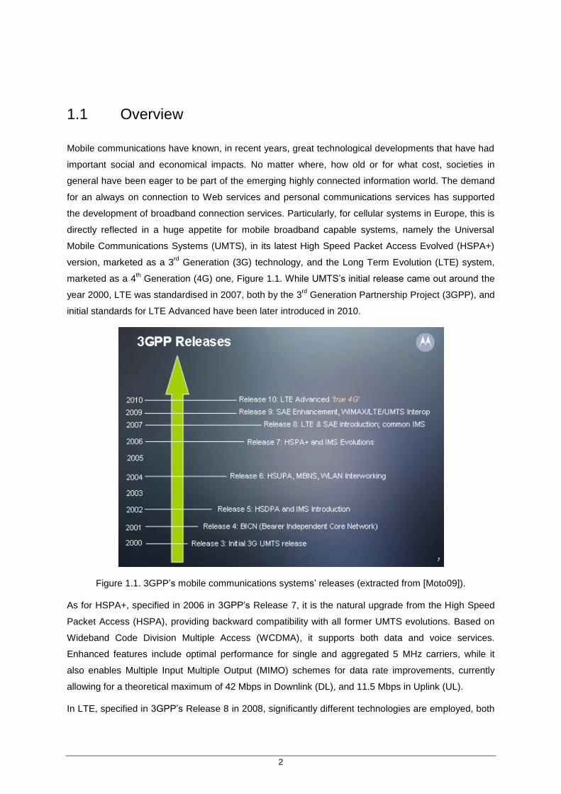
List of Figures Figure 1.1. 3GPP‟s mobile communications systems‟ releases (extracted from [Moto09]). .................... 2
Figure 1.2. Trends on the evolution of the telecom market. ..................................................................... 3
Figure 1.3. Mobile device data traffic multiplier, based on data equivalents of monthly feature phone traffic (adapted from [Cisc11]). ............................................................................ 4
Figure 2.1. UMTS network architecture (adapted from [HoTo07]). .......................................................... 8
Figure 2.2. Ninetieth percentile throughput as a function of Signal-to-Noise-Ratio (SNR) in Pedestrian A-channel (extracted from [BEGG08]) and Throughput as a function of in Pedestrian A channel (extracted from [PWST07]). .....................................11
Figure 2.3. Orthogonality factor, , as a function of user‟s distance to BS (extracted from [PeMo02]). ....................................................................................................................14
Figure 2.4. HSDPA data rate compared with the Shannon limit as a function of an average HS-DSCH carrier and interference power ratio (extracted from [HoTo06]). .......................17
Figure 2.5. Basic System Architecture of LTE (adapted from [HoTo09]). ..............................................18
Figure 2.6. DL frame structure type 1, for FDD and TDD (adapted from [Agil07]). ................................20
Figure 2.7. Inter-Cell Interference Coordination limit cases (extracted from [SeTB09]). .......................23
Figure 2.8. LTE spectral efficiency as a function of the geometry factor (extracted from [HoTo09]). .....................................................................................................................24
Figure 2.9. Throughput comparison between UMTS and LTE across the cell (extracted from [Moto10]). ......................................................................................................................26
Figure 2.10. Latency for different technologies (extracted from [Rysa10]). ...........................................27
Figure 3.1. Single-cell single-user model. ..............................................................................................32
Figure 3.2. Extending the single-cell single-user model to the multi-user case, by mapping other users and BSs as average intra- and inter-cell interference. .......................................35
Figure 3.3. Cell centre versus cell edge. ................................................................................................35
Figure 3.4. UMTS and LTE Simulator‟s architecture. .............................................................................36
Figure 3.5. Capacity and coverage performance results for UMTS and LTE UFR, for varying simulation period. ..........................................................................................................40
Figure 3.6. Capacity and coverage performance results for UMTS and LTE UFR, for varying number of users. ...........................................................................................................41
Figure 4.1. Measurements equipment used. ..........................................................................................48
Figure 4.2. Mobility measurements statistics for 0% cell load measurements over all the environments. ...............................................................................................................49
Figure 4.3. SINR statistics of DL static measurements results for different environments. ...................51
Figure 4.4. Throughput statistics of DL static measurements results for different environments. .........51
Figure 4.5. Transmission mode statistics analysis for static measurements in different environments. ...............................................................................................................52
Figure 4.6. Transmission mode analysis versus SINR and throughput, for mobility measurements in the Axial environment. .....................................................................52
Figure 4.7. Transmission mode versus SINR analysis, for mobility measurements in the Urban and Dense Urban environments. ..................................................................................53
Figure 4.8. CDFs of DL mobility and static measurements‟ results for the Urban environment. ...........53
Figure 4.9. Modulation schemes analysis in DL static measurements‟ results for different environments. ...............................................................................................................55
Figure 4.10. Serving and neighbouring cell RSRP difference as a function of distance to BS for
xii
the Axial environment, based on mobility measurements. ...........................................56
Figure 4.11. Cell edge versus cell edge statistics, from mobility measurements in the Urban environment. .................................................................................................................56
Figure 4.12. CDFs of DL measurements results, for varying load, in the Urban environment. .............57
Figure 4.13. Modulation schemes average use regarding cell load for the Axial environment. .............58
Figure 4.14. Modulation schemes average use regarding cell load for the Urban and Dense Urban environments. ....................................................................................................58
Figure 4.15. Performance differences between cell centre and cell edge as a function of cell load, for varying environment. ......................................................................................59
Figure 4.16. Link loss, average SINR and average throughput as a function of distance to serving BS. ....................................................................................................................60
Figure 4.17. Average DL throughput as a function of average SINR. ....................................................60
Figure 4.18. Simulated and measured results, respectively for the pedestrian channel and static measurements. .............................................................................................................61
Figure 4.19. Simulated and measured results for the Urban vehicular scenario in DL, for varying load. ..............................................................................................................................62
Figure 4.20. Simulated and measured performance differences between cell centre and cell edge in the Urban vehicular scenario, for varying load. ...............................................63
Figure 4.21. LTE and UMTS DL SINR for the Urban pedestrian scenario, for varying users‟ number. .........................................................................................................................64
Figure 4.22. LTE and UMTS DL throughput for the Axial pedestrian scenario, for varying users‟ number. .........................................................................................................................64
Figure 4.23. LTE and UMTS DL throughput for the Urban pedestrian scenario, for varying users‟ number. .........................................................................................................................65
Figure 4.24. LTE and UMTS DL throughput for the Dense Urban pedestrian scenario, for varying users‟ number. .................................................................................................65
Figure 4.25. UMTS to LTE throughput ratio for the Urban pedestrian scenario, for varying users‟ number. .........................................................................................................................66
Figure 4.26. LTE and UMTS coverage results for the Urban pedestrian scenario, for required 1Mbps and 5Mbps throughput service..........................................................................67
Figure 4.27. LTE and UMTS coverage results for the Urban pedestrian scenario, for required 10Mbps throughput service. .........................................................................................67
Figure 4.28. Performance differences between cell centre to cell edge for the pedestrian channel with LTE UFR. .................................................................................................69
Figure 4.29. LTE and UMTS UL SINR for the Urban pedestrian scenario, for varying users‟ number. .........................................................................................................................70
Figure 4.30. LTE and UMTS UL throughput for the Axial pedestrian scenario, for varying users‟ number. .........................................................................................................................71
Figure 4.31. LTE and UMTS UL throughput for the Urban and Dense Urban pedestrian scenarios, for varying users‟ number. ...........................................................................71
Figure 4.32. UMTS to LTE throughput ratio for the Urban pedestrian scenario, for varying users‟ number. .........................................................................................................................72
Figure 4.33. LTE and UMTS coverage results for the Urban pedestrian scenario, for required 1Mbps and 5Mbps throughput service..........................................................................72
Figure 4.34. LTE and UMTS coverage results for the Urban pedestrian scenario, for required 10Mbps throughput service. .........................................................................................73
Figure 4.35. Performance difference between cell centre to cell edge in the LTE UFR Urban pedestrian scenario, for varying number of users in the cell. .......................................74
Figure B.1. HSPA+ DL with MIMO configurations – SNR as a function of physical Throughput (extracted from [Jaci09]). ..............................................................................................90
Figure B.2. HSPA+ UL for 16QAM – as a function of physical Throughput (extracted from [Jaci09]). .......................................................................................................................90
Figure B.3. HSPA+ DL with MIMO and SISO configurations – physical Throughput as a function
xiii
of SNR (extracted from [Jaci09]). .................................................................................92
Figure B.4. HSPA+ UL for 16QAM – physical Throughput as a function of SNR (extracted from [Jaci09]). .......................................................................................................................93
Figure B.5. Channel and transmission bandwidth configuration for a LTE carrier (extracted from [Khan09]) ......................................................................................................................95
Figure B.6. LTE EPA5Hz downlink physical throughput per RB for two layer 16QAM and 64QAM modulation schemes as a function of SNR. ..................................................101
Figure B.7. LTE EPA5Hz uplink physical throughput per RB for two layer 16QAM and 64QAM modulation schemes as a function of SNR. ................................................................104
Figure C.1. COST231 Walfisch-Ikegami assumptions and associated definition parameters (extracted from [Corr10]). ...........................................................................................105
Figure D.1. Different radio transmission schemes, SISO, SIMO, MISO and MIMO (adapted from [Agil11]). ......................................................................................................................109
Figure D.2. Average SINR, rank 1 SINR and rank 2 SINR levels (extracted from [Opti11]). ...............110
Figure E.1. Main simulator window: simulation parameters, channel, propagation model, systems' and output results path definition.. ...............................................................115
Figure E.2. UMTS/HSPA+ parameters input window...........................................................................116
Figure E.3. LTE parameters input window. ..........................................................................................117
Figure E.4. Channel model and Propagation Model parameters input windows. ................................117
Figure F.1. SINR statistics of DL mobility measurements results for different environments. .............119
Figure F.2. Throughput statistics of DL mobility measurements results for different environments. .............................................................................................................120
Figure F.3. Transmission mode statistics analysis for mobility measurements in different environments. .............................................................................................................120
Figure F.4. SINR statistics for average SINR, Rank1 SINR and RANK2 SINR, from mobility measurements in the Axial environment. ...................................................................121
Figure F.5. CDFs of DL mobility and static measurements‟ results for the Axial environment. ...........121
Figure F.6. CDFs of DL mobility and static measurements results for the Dense Urban environment. ...............................................................................................................121
Figure F.7. Average modulation usage analysis of DL mobility measurements‟ results for different environments. ...............................................................................................122
Figure F.8. Cell edge versus cell edge statistics, from mobility measurements in the Axial environment. ...............................................................................................................122
Figure F.9. Cell edge versus cell edge statistics, from mobility measurements in the Dense Urban environment. ....................................................................................................122
Figure F.10. CDFs of DL measurements results, for varying load, in the Axial environment. .............123
Figure F.11. CDFs of DL measurements results, for varying load, in the Dense Urban environment. ...............................................................................................................123
Figure F.12. Transmission mode average use regarding cell load, for different environments. ..........124
Figure F.13. Cell centre versus cell edge average SINR and average throughput as a function of load, for the Axial environment. ..................................................................................124
Figure F.14. Cell centre versus cell edge average SINR and average throughput as a function of load, for the Urban and Dense Urban environments. .................................................125
Figure F.15. DL SINR PDFs of measured and simulated results for the Axial pedestrian scenario. .....................................................................................................................125
Figure F.16. DL SINR PDFs of measured and simulated results for the pedestrian channel of the Urban and Dense Urban environments. ...............................................................125
Figure F.17. Simulated and measured results for the Axial vehicular scenario in DL, for varying load. ............................................................................................................................126
Figure F.18. Simulated and measured results for the Dense Urban vehicular scenario in DL, for varying load. ................................................................................................................126
Figure F.19. Simulated and measured results for the difference between cell centre to cell edge in the Axial vehicular scenario, for varying load. ........................................................126
xiv
Figure F.20. Simulated and measured results for the difference between cell centre to cell edge DL in the Dense Urban vehicular scenario, for varying load. .....................................127
Figure F.21. Simulated cell edge versus cell centre results for DL of the Axial vehicular scenario, for varying load. ...........................................................................................127
Figure F.22. Simulated cell edge versus cell centre results for DL of the Urban vehicular scenario, for varying load. ...........................................................................................127
Figure F.23. Simulated cell edge versus cell centre results for DL of the Dense Urban vehicular scenario, for varying load. ...........................................................................................128
Figure F.24. LTE and UMTS DL SINR for the Axial and Dense Urban pedestrian scenarios, for varying users‟ number. ...............................................................................................128
Figure F.25. UMTS to LTE throughput ratio for the Axial and Dense Urban pedestrian scenarios, for varying users‟ number. ..........................................................................................129
Figure F.26. LTE and UMTS coverage results for LTE UFR‟s DL in the pedestrian scenario, for required 1Mbps and 5Mbps throughput service. ........................................................129
Figure F.27. LTE and UMTS coverage results for LTE UFR‟s DL in the pedestrian scenario, for required 10Mbps throughput service. .........................................................................129
Figure F.28. Cell centre to cell edge reduction in the Urban pedestrian scenario for UMTS DL, when varying number of users. ...................................................................................130
Figure F.29. Performance difference between cell centre to cell edge DL in the LTE ICIC Urban pedestrian scenario, for varying number of users in the cell. .....................................130
Figure F.30. SINR and throughput, in DL, as a function of distance to BS, for the Urban pedestrian scenario with a single cell user. ................................................................130
Figure F.31. LTE and UMTS UL SINR for the Axial and Dense Urban pedestrian scenarios, for varying users‟ number. ...............................................................................................131
Figure F.32. UMTS to LTE throughput ratio for the Axial and Dense Urban pedestrian scenarios, for varying users‟ number. ..........................................................................................131
Figure F.33. LTE and UMTS coverage results for LTE UFR‟s UL in the pedestrian scenario, for required 1Mbps and 5Mbps throughput service. ........................................................131
Figure F.34. LTE and UMTS coverage results for LTE UFR‟s UL in the pedestrian scenario, for required 10Mbps throughput service. .........................................................................132
Figure F.35. Cell centre to cell edge reduction in the Urban pedestrian scenario for UMTS UL, when varying number of users. ...................................................................................132
Figure F.36. Cell centre to cell edge reduction in the Axial pedestrian scenario for LTE, for varying number of users in the cell. ............................................................................132
Figure F.37. Cell centre to cell edge reduction in the Dense Urban pedestrian scenario for LTE, for varying number of users in the cell. .......................................................................133
Figure F.38. SINR and throughput, in UL, as a function of distance to BS, for the Urban pedestrian scenario with a single cell user. ................................................................133
Figure G.1. Outdoor LTE Cluster in Porto (extracted from [GoEa11]). ................................................135
Figure G.2. Inter-BS distance, measured as the distance to the closest detected cell, for the Axial environment (extracted from [GoEa11] ). ..........................................................135
Figure G.3. Inter-BS distance, measured as the distance to the closest detected cell, for the Urban environment (extracted from [GoEa11]). .........................................................136
Figure G.4. Inter-BS distance, measured as the distance to the closest detected cell, for the Dense Urban environment (extracted from [GoEa11] ). .............................................136
Figure G.5. Drive tests‟ and static measurements‟ spots results, sorted by DL throughput (extracted from [GoEa11]). .........................................................................................137
Figure G.6. Drive tests‟ route for coverage analysis, sorted by DL throughput (extracted from [GoEa11]). ...................................................................................................................137
xv
List of Tables
List of Tables Table 2.1. Benchmarking of Dual carrier HSDPA and MIMO (adapted from [HoTo09]). .......................12
Table 2.2. Feature comparison of the HSPA+ achievements in DL and UL directions. ........................12
Table 2.3. DL user throughput performance for 500 m Inter-Site Distances (ISD), (adapted from [3GPP09]). ....................................................................................................................26
Table 2.4. DL and UL spectrum efficiency performance 500 m ISD (adapted from [3GPP09]). ...........27
Table 2.5. Major features comparison, under analysis in this thesis, between UMTS and LTE (adapted from [HoTo07], [HoTo09], [Moto07] and [ANAC11]). ....................................28
Table 3.1. User throughput and distance to BS for 1 Mbps and 5 Mbps data rates in UMTS. ..............41
Table 3.2. User throughput and distance to BS for 1 Mbps and 5 Mbps data rates in LTE UFR. .........42
Table 4.1. COST231-Walfisch-Ikegami‟s environment parameters for the urban scenarios, [Opti11]. ........................................................................................................................44
Table 4.2.Default values used in UMTS and LTE link budgets (based on [Jaci09], [EsPe06], [HoTo09], [PoPo10] and [Opti11]). ...............................................................................45
Table 4.3. Neighbouring BS‟s transmitted power, regarding cell load, [Opti11]. ....................................47
Table 4.4.Default required service data rates considered for coverage analysis (based on [Jaci09] and [Pere11]). ..................................................................................................47
Table 4.5. Equipment used in LTE live measurements. .........................................................................48
Table 4.6. SINR‟s and throughput‟s mean and standard deviation, for different environments. ............51
Table 4.7. SINR‟s and throughput‟s mean and standard deviation for static and mobility scenarios. ......................................................................................................................54
Table 4.8. SINR‟s and throughput‟s mean and standard deviation for cell edge versus cell centre, for the mobility scenario. ...................................................................................56
Table 4.9. SINR‟s and throughput‟s mean and standard deviation for varying load scenarios in the Urban environment. ................................................................................................57
Table 4.10. Correlation coefficients between measured and simulated results, for varying environment. .................................................................................................................62
Table 4.11. Correlation coefficients between measured and simulated results of cell centre to cell edge reduction, for varying environment in mobility. ..............................................63
Table A.1. Distributions and standard deviations for slow and fast fading margins (extracted from [Jaci09]). ...............................................................................................................84
Table A.2. Rice parameter (based on [GGEM09]). ................................................................................84
Table A.3. Channel coherence time values. ...........................................................................................85
Table B.1. Characterisation of the channel models used, in terms of Doppler frequency spread and delay spread (extracted from [Jaci09]). .................................................................93
Table B.2. Extrapolation EVA5Hz to EPA5Hz (extracted from [Duar08]). .............................................94
Table B.3. Transmission band (adapted from [Duar08]). .......................................................................94
Table D.1. Decision matrix for the main LTE MIMO modes (adapted from [Tele09]). .........................111
Table D.2. Mean value of for systems with =2, independent of cell type (extracted from [KuCo08]). ...........................................................................................................112
Table D.3. Mean value of for systems with >2 and >2 for different cell types ([KuCo08]). ..................................................................................................................112
Table D.3 (cont.). Mean value of for systems with >2 and >2 for different cell types ([KuCo08]). ..................................................................................................................113
Table F.1. Distance to serving BS mean and standard deviation, for different environments. ............119
xvi
Table F.2. ISDs for varying environment. .............................................................................................119
Table F.3. SINR‟s and throughput‟s mean and standard deviation of DL mobility measurements, for different environments. ..........................................................................................120
Table F.4. Serving cell and detected cell RSRP difference given as a function of distance to BS, obtained by curve fitting. .............................................................................................120
Table F.5. SINR‟s and throughput‟s mean and standard deviation for varying load scenarios in the Axial environment. ................................................................................................123
Table F.6. SINR‟s and throughput‟s mean and standard deviation for varying load scenarios in the Dense Urban environment. ...................................................................................124
Table F.7. Average throughput ratio as a function of number of cell users, obtained by curve fitting. ..........................................................................................................................128
xvii
List of Acronyms
List of Acronyms 3G 3rd Generation
3GPP 3rd Generation Partnership Project
4G 4th Generation
AMC Adaptive Modulation Coding
AWGN Additive White Gaussian Noise
BER Bit Error Rate
BLER Block Error Rate
BS Base Station
CCH Common Channel
CDF Cumulative Distribution Function
CDMA Code Division Multiple Access
CN Core Network
CP Cyclic Prefix
CPC Continuous Packet Connectivity
CQI Channel Quality Indication
CS Circuit-Switched
CSI Channel State Information
CSV Comma-Separated Values
DCH Dedicated Channel
DL Downlink
DPCCH Dedicated Physical Control Channel
DPCH Dedicated Physical Channels
DS-CDMA Direct-Sequence CDMA
DSCH Downlink Shared Channel
E-DCH Evolved-DCH
EIRP Equivalent Isotropic Radiated Power
eNB Evolved Node B
EPA Extended Pedestrian A
EPC Evolved Packet Core Network
EPS Evolved Packet System
ETU Extended Typical Urban
E-UTRAN Evolved UTRAN
EVA Extended Vehicular A
FACH Forward Access Channel
xviii
FDD Frequency Division Duplexing
FTP File Transfer Protocol
GBSB Geometrically Based Single Bounce
GGSN Gateway GPRS Support Node
GMSC Gateway MSC
GPRS General Packet Radio Service
GSM Global System for Mobile Communications
GUI Graphical User Interface
HARQ Hybrid Automatic Repeat Request
HLR Home Location Register
HO Handover
HOM Higher Order Modulation
HSDPA High Speed Downlink Packet Access
HS-DPCCH High-Speed Dedicated Physical Control Channel
HS-DSCH High-Speed Downlink Shared Channel
HSPA High Speed Packet Access
HSPA+ HSPA Evolution
HS-PDSCH High-Speed Physical Downlink Shared Channel
HSS Home Subscription Server
HS-SCCH High-Speed Shared Control Channel
HSUPA High Speed Uplink Packet Access
ICIC Inter-Cell Interference Coordination
IMS IP Multimedia Sub-system
IP Internet Protocol
IPTV IP Television
ISD Inter-Site Distance
ISI Inter-Symbol Interference
L1 Layer-1
L2 Layer-2
LoS Line of Sight
LTE Long Term Evolution
MAC Medium Access Control
MBMS Multimedia Broadcast Multicast Service
MCS Modulation and Coding Scheme
ME Mobile Equipment
MIMO Multiple Input Multiple Output
MISO Multiple Input Single Output
MM Mobility Management
MME Mobility Management Entity
MRC Maximal Ratio Combining
xix
MMOG Multimedia Online Gaming
MSC Mobile Switching Centre
MT Mobile Terminal
NB Node B
NLoS Non-LoS
OFDM Orthogonal Frequency Division Multiplexing
OFDMA Orthogonal Frequency Division Multiple Access
OLSM Open Loop Spatial Multiplexing
OVSF Orthogonal Variable Spreading Factor
PAR Peak-to-Average-power-Ratio
PBCH Physical Broadcast Channel
P-CPICH Primary Common Pilot Channel
PCRF Policy and Charging Resource Function
PDCCH Physical Downlink Control Channel
PDSCH Physical Downlink Shared Channel
PDU Protocol Data Unit
P-GW Packet Data Network Gateway
PMI Pre-coding Matrix Indicator
PRACH Physical Random Access Channel
PS Packet-Switched
PSS Primary Synchronisation Signal
PUCCH Physical Uplink Control Channel
PUSCH Physical Uplink Shared Channel
QAM Quadrature Amplitude Modulation
QoS Quality of Service
QPSK Quadrature Phase Shift Keying
RACH Random Access Channel
RB Resource Block
RF Radio Frequency
RI Rank Indicator
RLC Radio Link Control
RMG Relative MIMO Gain
RNC Radio Network Controller
RRC Radio Resource Control
RRM Radio Resource Management
RSRP Reference Signal Reference Power
RTT Round Trip Time
SAE System Architecture Evolution
SAE-GW SAE Gateway
SC-FDMA Single Carrier Frequency Division Multiple Access
xx
SF Spreading Factor
SFBC Space-Frequency Block Coding
SGSN Serving GPRS Support Node
S-GW Serving Gateway
SIMO Single Input Multiple Output
SINR Signal-to-Interference-plus-Noise Ratio
SIR Signal-to-Interference-Ratio
SISO Single Input Single Output
SNR Signal-to-Noise-Ratio
SSS Secondary Synchronisation Signal
TDD Time Division Duplexing
TTI Transmission Time Interval
UE User Equipment
UFR Universal Frequency Reuse
UL Uplink
UMTS Universal Mobile Telecommunications System
USIM UMTS Subscriber Identity Mobile
UTRAN UMTS Terrestrial Radio Access Network
VLR Visitor Location Register
VoIP Voice over IP
WCDMA Wideband CDMA
WiMAX Worldwide Interoperability for Microwave Access
xxi
List of Symbols
List of Symbols
Downlink orthogonality factor
Subcarrier activity factor of cell
Subcarrier spacing
Mean relative error
Mean square error
Load factor
Average DL load factor value across the cell
Scheduler efficiency
Mean value
Non-centrality parameter of the Rice distribution
SNR
SNIR
SNR employing ICIC schemes
Incidence angle
Standard deviation
Fast fading coherence time
Slow fading coherence time
Average power decay
Bandwidth of the total RBs allocated, in LTE, or , in UMTS
Bandwidth allocated to user
Average bandwidth of the RBs allocated per user
Capacity of the MIMO system
Correlation between random variables and
Covariance between random variables and
Capacity of the SISO system
Distance between user and BS
Energy per bit
Energy per chip stream
Frequency
Noise figure of the receiver
Array gain
Diversity gain
xxii
ICIC scheme gain
Relative MIMO Gain
Masthead amplifier gain
Capacity gain obtained due to multi-user diversity
Processing gain
Capacity gain obtained due to users‟ positioning in the cell
Gain of the receiving antenna, including diversity
Gain of the receiving antenna
Relative SIMO gain
Gain of the transmitting antenna
BS height
Buildings‟ height
Channel gain from the serving cell to user , transmitting in RB
Channel gain from the serving cell to user , transmitting in
RB
MT height
Ratio of inter- to intra-cell interferences power
Rice parameter
Dependence of the multiscreen diffraction loss versus distance
Free space loss
COST231-Walfisch-Ikegami propagation losses
Link loss
Cable losses between transmitter and antenna
Pathloss
Pathloss due to indoor propagation
Pathloss from serving BS to user
Pathloss from user in cell to the serving BS
Pathloss from BS to the user
Maximum pathloss without attenuation or losses
Pathloss due to outdoor propagation
Total pathloss
Propagation model losses
Approximation for the multi-screen diffraction loss
Rooftop-to-street diffraction and scatter loss
User losses
Modulation order
Total margin
Total fading margin
xxiii
Fast fading margin
Interference margin
Average interference margin
Slow fading margin
Total noise power
Noise power spectral density
Number of neighbouring BSs
Number of receiving antennas
Number of RBs used in DL
Number of RBs used in UL
Number of user RBs
Noise power at the receiver
Timing offset between UL and DL radio frames at the UE in units of
Ratio between users close to eNB and total number of users
Number of subcarriers per resource block
Number of MIMO streams
Number of symbols per sub-frame
Number of symbols per time slot
Number of transmitting antennas
Number of users
Number of samples of dataset
Interference power
Received inter-cell interference power
Received DL inter-cell interference power
Received UL inter-cell interference power
Received intra-cell interference power
Received DL intra-cell interference power
Received UL intra-cell interference power
Maximum interference power of cell
Total transmission power
Total BS transmitted power
BS transmitted power to user
BS transmitted power
UE transmitted power to BS
Transmitted power from user in adjacent cell
Power allocated to the common channels
Power allocated to the dedicated channels
xxiv
Transmit power from cell , transmitting in RB
Transmit power from cell , transmitting in RB
Received power of the DSCH
Received power of HS-DSCH
Receiver sensitivity
Signalling and control power
Power available at the receiving antenna
Power fed to the transmitting antenna
Cell radius
Data bit rate
Average user data bit rate
Chip rate
HS-PDSCH Spreading Factor of 16
Sample period
Sub-frame period
Time slot duration
User activity factor
Average user activity factor
Mean value of
Inter Buildings Distance
Street width
Sample of variable
xxv
List of
List of Software MATLAB Computational Math Tool
Microsoft Visual C++ 2010 ANSI C++ Integrated Development Environment
Microsoft Excel 2007 Calculation and graphical chart tool
Microsoft Word 2007 Text editor software
Microsoft Powerpoint 2007 Presentation software
Microsoft Visio 2007 Design tool (e.g. diagrams, flowcharts, etc)

xxvi

1
Chapter 1
Introduction
1 Introduction
The present chapter introduces the theme of this dissertation, in particular, over a contextual and
motivational perspective, while simultaneously providing an overview of the assumptions established
for the work development. Furthermore, it establishes the scope for the work performed together with
its main contributions, followed by the detailed presentation of the work‟s structure.
2
1.1 Overview
Mobile communications have known, in recent years, great technological developments that have had
important social and economical impacts. No matter where, how old or for what cost, societies in
general have been eager to be part of the emerging highly connected information world. The demand
for an always on connection to Web services and personal communications services has supported
the development of broadband connection services. Particularly, for cellular systems in Europe, this is
directly reflected in a huge appetite for mobile broadband capable systems, namely the Universal
Mobile Communications Systems (UMTS), in its latest High Speed Packet Access Evolved (HSPA+)
version, marketed as a 3rd
Generation (3G) technology, and the Long Term Evolution (LTE) system,
marketed as a 4th Generation (4G) one, Figure 1.1. While UMTS‟s initial release came out around the
year 2000, LTE was standardised in 2007, both by the 3rd
Generation Partnership Project (3GPP), and
initial standards for LTE Advanced have been later introduced in 2010.
Figure 1.1. 3GPP‟s mobile communications systems‟ releases (extracted from [Moto09]).
As for HSPA+, specified in 2006 in 3GPP‟s Release 7, it is the natural upgrade from the High Speed
Packet Access (HSPA), providing backward compatibility with all former UMTS evolutions. Based on
Wideband Code Division Multiple Access (WCDMA), it supports both data and voice services.
Enhanced features include optimal performance for single and aggregated 5 MHz carriers, while it
also enables Multiple Input Multiple Output (MIMO) schemes for data rate improvements, currently
allowing for a theoretical maximum of 42 Mbps in Downlink (DL), and 11.5 Mbps in Uplink (UL).
In LTE, specified in 3GPP‟s Release 8 in 2008, significantly different technologies are employed, both
3
in the air interface and core network, aiming at bringing higher spectral efficiency and the network
closer to the world of Internet Protocol (IP). LTE uses Orthogonal Frequency Division Multiplexing
(OFDM) for radio access, together with more advanced MIMO schemes, providing for theoretical
maximum data rates of 326 Mbps and 86 Mbps, for DL and UL, respectively.
Performance and usability of mobile handsets has improved together with a wide adoption of 3G
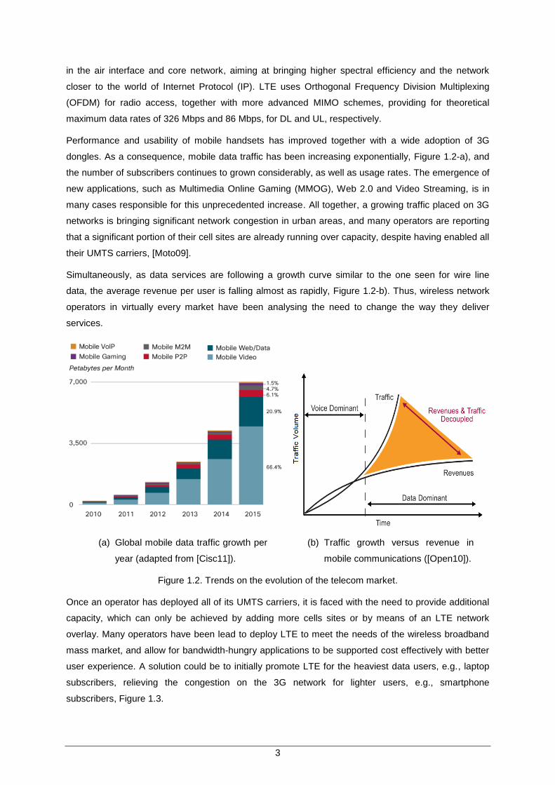
dongles. As a consequence, mobile data traffic has been increasing exponentially, Figure 1.2-a), and
the number of subscribers continues to grown considerably, as well as usage rates. The emergence of
new applications, such as Multimedia Online Gaming (MMOG), Web 2.0 and Video Streaming, is in
many cases responsible for this unprecedented increase. All together, a growing traffic placed on 3G
networks is bringing significant network congestion in urban areas, and many operators are reporting
that a significant portion of their cell sites are already running over capacity, despite having enabled all
their UMTS carriers, [Moto09].
Simultaneously, as data services are following a growth curve similar to the one seen for wire line
data, the average revenue per user is falling almost as rapidly, Figure 1.2-b). Thus, wireless network
operators in virtually every market have been analysing the need to change the way they deliver
services.
(a) Global mobile data traffic growth per
year (adapted from [Cisc11]).
(b) Traffic growth versus revenue in
mobile communications ([Open10]).
Figure 1.2. Trends on the evolution of the telecom market.
Once an operator has deployed all of its UMTS carriers, it is faced with the need to provide additional
capacity, which can only be achieved by adding more cells sites or by means of an LTE network
overlay. Many operators have been lead to deploy LTE to meet the needs of the wireless broadband
mass market, and allow for bandwidth-hungry applications to be supported cost effectively with better
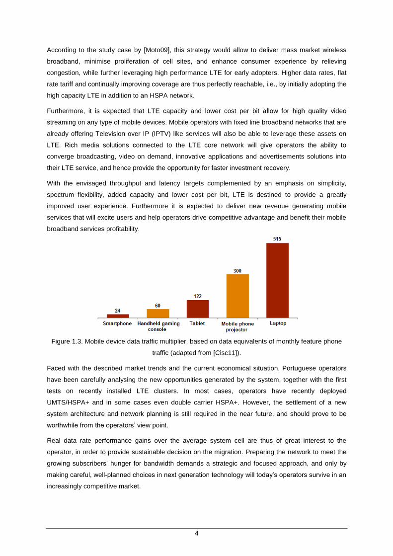
user experience. A solution could be to initially promote LTE for the heaviest data users, e.g., laptop
subscribers, relieving the congestion on the 3G network for lighter users, e.g., smartphone
subscribers, Figure 1.3.
4
According to the study case by [Moto09], this strategy would allow to deliver mass market wireless
broadband, minimise proliferation of cell sites, and enhance consumer experience by relieving
congestion, while further leveraging high performance LTE for early adopters. Higher data rates, flat
rate tariff and continually improving coverage are thus perfectly reachable, i.e., by initially adopting the
high capacity LTE in addition to an HSPA network.
Furthermore, it is expected that LTE capacity and lower cost per bit allow for high quality video
streaming on any type of mobile devices. Mobile operators with fixed line broadband networks that are
already offering Television over IP (IPTV) like services will also be able to leverage these assets on
LTE. Rich media solutions connected to the LTE core network will give operators the ability to
converge broadcasting, video on demand, innovative applications and advertisements solutions into
their LTE service, and hence provide the opportunity for faster investment recovery.
With the envisaged throughput and latency targets complemented by an emphasis on simplicity,
spectrum flexibility, added capacity and lower cost per bit, LTE is destined to provide a greatly
improved user experience. Furthermore it is expected to deliver new revenue generating mobile
services that will excite users and help operators drive competitive advantage and benefit their mobile
broadband services profitability.
Figure 1.3. Mobile device data traffic multiplier, based on data equivalents of monthly feature phone
traffic (adapted from [Cisc11]).
Faced with the described market trends and the current economical situation, Portuguese operators
have been carefully analysing the new opportunities generated by the system, together with the first
tests on recently installed LTE clusters. In most cases, operators have recently deployed
UMTS/HSPA+ and in some cases even double carrier HSPA+. However, the settlement of a new
system architecture and network planning is still required in the near future, and should prove to be
worthwhile from the operators‟ view point.
Real data rate performance gains over the average system cell are thus of great interest to the
operator, in order to provide sustainable decision on the migration. Preparing the network to meet the
growing subscribers‟ hunger for bandwidth demands a strategic and focused approach, and only by
making careful, well-planned choices in next generation technology will today‟s operators survive in an
increasingly competitive market.
5
1.2 Motivation and Contents
The main scope of this thesis is to compare two systems: UMTS/HSPA+ and LTE. As LTE looks for its
place as the successor to UMTS, an analysis of the system‟s transmission characteristics over varying
environment, channel, cell load and coverage for different services is determinant for migration
analysis. Therefore, the aim of the analysis is to study, for both DL and UL, capacity and coverage
aspects, taking data rate gains as a reference.
The main contribution of this thesis is the development of a model for two different analysis: one to
evaluate maximum data rates obtained, allowing for computing data rate gains from UMTS/HSPA+ to
LTE, and the other to analyse maximum cell range, providing the use of a given service. Supported by
measurements performed in a live LTE network, one can have a very good comparison of the two
technologies at stake.
For work development, a partnership was established with Optimus, a Portuguese mobile operator.
The collaboration had the important role of providing assistance on several technical details and
insights on the technologies, as well as supporting the measurements‟ campaign performed.
The present thesis is composed of 5 chapters, including the present one. Chapter 2 presents an
introduction to UMTS/HSPA+ and LTE. UMTS basic concepts are overviewed, and key features of the
releases under study emphasised. Particularly, radio interface measurement grades are out looked,
regarding coverage and capacity. A similar analysis follows then, for LTE, in a subsequent section. At
the end, a full side by side comparison of the two systems is presented, enhancing key strengths and
weaknesses of the two systems, followed by an overview of the current state of the art on the topic.
Chapter 3 introduces the developed models used for simulation. The single cell model is explained, for
both single- and multi-user scenarios, for analysis over different channel, environment, cell load and
service coverage scenarios. UMTS and LTE systems‟ modules developed for both DL and UL are also
described together with the propagation and channel simulation modules. The simulator assessment
is presented at the end.
In Chapter 4, LTE measurements‟ and simulations‟ single-user results are taken under an exhaustive
analysis, where the influence of varying environment, channel and cell load is mainly considered.
Finally the full comparison with capacity and coverage results for UMTS/HSPA+ is done, for a multi-
user scenario, and for both DL and UL.
Chapter 5 concludes the present dissertation, where a critical analysis is drawn followed by the main
work conclusions. Furthermore, suggestions for future work are outlined and paths for further research
on next generation mobile communications‟ solutions are enlightened. Finally, a set of annexes closes
the present document, with supplementary information, when the need for the global comprehension
of the problem exists.

7
Chapter 2
Basic Concepts
2 Models
This chapter provides an overview of UMTS, focusing on system architecture, radio interface,
coverage and capacity, and general performance. In the following the LTE system is analysed in a
similar way, drawing comparisons with UMTS. Finally, a brief comparison between the two systems is
drawn and state of the art on the subject presented.
8
2.1 UMTS
This section overviews the fundamental concepts regarding UMTS in its most recent form. First, the
system architecture is presented, together with its main elements. A brief description of the radio
interface follows, basic concepts of coverage and capacity are overviewed, and finally a performance
analysis is drawn. This section is based on [HoTo07] and [3GPP10a].
2.1.1 Network Architecture
UMTS‟s network architecture, Figure 2.1 was first defined in 3GPP‟s Release99, remaining
unchanged in later releases. It consists of a number of network elements that can be grouped into
three sub-networks: User‟s Equipment (UE), UMTS Terrestrial Radio Access Network (UTRAN) and
Core Network (CN).
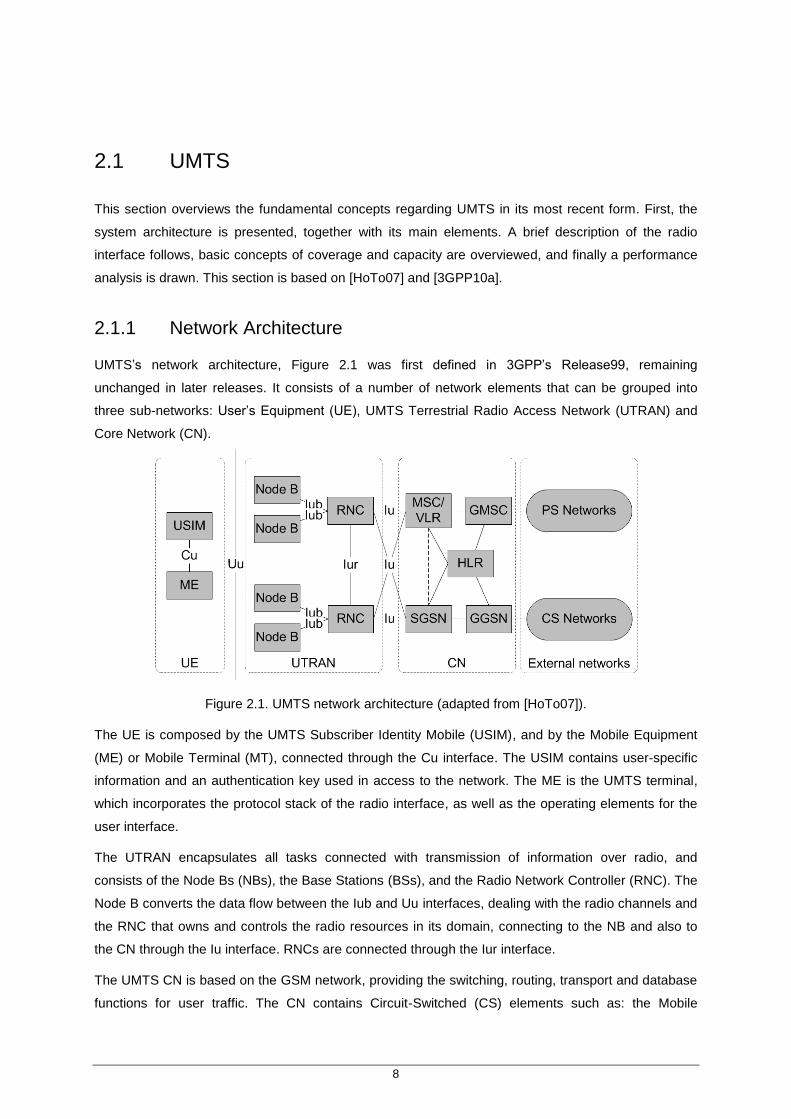
Figure 2.1. UMTS network architecture (adapted from [HoTo07]).
The UE is composed by the UMTS Subscriber Identity Mobile (USIM), and by the Mobile Equipment
(ME) or Mobile Terminal (MT), connected through the Cu interface. The USIM contains user-specific
information and an authentication key used in access to the network. The ME is the UMTS terminal,
which incorporates the protocol stack of the radio interface, as well as the operating elements for the
user interface.
The UTRAN encapsulates all tasks connected with transmission of information over radio, and
consists of the Node Bs (NBs), the Base Stations (BSs), and the Radio Network Controller (RNC). The
Node B converts the data flow between the Iub and Uu interfaces, dealing with the radio channels and
the RNC that owns and controls the radio resources in its domain, connecting to the NB and also to
the CN through the Iu interface. RNCs are connected through the Iur interface.
The UMTS CN is based on the GSM network, providing the switching, routing, transport and database
functions for user traffic. The CN contains Circuit-Switched (CS) elements such as: the Mobile
9
Switching Centre (MSC), a central switching node of the CS domain of the CN, responsible for
switching the CS transactions, namely voice; and the Gateway MSC (GMSC), a switch on the
connection between the CN and the external CS networks. Regarding Packet-Switched (PS) elements
it includes: the Serving General Packet Radio Service (GPRS) Support Node (SGSN), a central
switching node of the PS domain in the CN, responsible for the delivery of data packets from and to
the BSs; and the Gateway GPRS Support Node (GGSN), a switch with functionality close to that of
GMSC, but connecting the CN to the external PS networks.
Furthermore, two elements exist that are both CS and PS based: theHome Location Register (HLR), a
database located in the users‟ home system that stores the users‟ service profiles, such as associated
authorisations and keys in a connection; and the Visitor Location Register (VLR), a distributed
database that saves temporary information about the active users in the geographical area allocated
to it, preventing the central database to be interrogated for all the subscriber information each time a
new subscriber roams into a location area.
2.1.2 Radio Interface
UMTS‟s WCDMA radio interface is based on Direct-Sequence Code Division Multiple Access (DS-
CDMA), a spread spectrum air interface, with a chip rate of 3.84 Mcps leading to a radio channel of
4.4 MHz and separation of 5 MHz. This access method allows for very high and variable bandwidths,
low delay, smooth mobility for voice and packet data and inter-working with existing GSM/GPRS
networks. As defined in [3GPP10a], in 3GPP‟s Release 99, the frequency bands for Europe are
[1920, 1980] MHz for UL and [2110, 2170] MHz for DL.
In UMTS, two types of codes are used for spreading and WCDMA multiple access: channelisation and
scrambling, [Corr08]. Channelisation codes are used in DL for UE separation, whilst in UL they
distinguish between physical data and control channels. The sequence of chips is multiplied by the
user‟s information, associating to a spreading factor the use of an Orthogonal Variable Spreading
Factor (OVSF) code, and obtaining a wide spectrum signal. Codes allow to maintain orthogonality
between them and to vary the Spreading Factor (SF). Scrambling is used on top of spreading, so it
does not change the signal bandwidth, and enables sector separation in DL, and UE separation in UL.
UMTS also provides for power management and soft and softer handovers. Power management is
achieved using closed loop power control in both UL, to avoid using excessive power and increasing
interference, and DL, taking in account a margin of the cell limits, and using outer loop power control
to dynamically adjust the Signal-to-Interference-Ratio (SIR), saving in system capacity. Soft and softer
Handovers (HOs) take place in a user transition between cells or sectors of a cell, respectively,
allowing for the combining of the received user signal in the RNC or BS, respectively.
High Speed Downlink Packet Access (HSDPA) and High Speed Uplink Packet Access (HSUPA),
together known as HSPA, are evolutions of 3GPP‟s Release 99 being defined in Release 5 and
Release 6, respectively. With HSDPA, scheduling control and link adaptation based on physical layer
retransmissions were moved from the RNC to the BS, guaranteeing fast link adaptation and fast
channel-dependent scheduling, [HoTo09]. Furthermore, the duration of the transmission, named
10
Transmission Time Interval (TTI), is defined to be 2 ms to achieve a short round-trip delay for the
operation between UE and BS for retransmissions, [HoTo07].
For user data transmission, a fixed SF of 16 is specified for HSDPA, as 15 channelisation codes are
available per UE in the High-Speed Physical Downlink Shared Channel (HS-PDSCH), and the last
channelisation code is reserved for the High-Speed Shared Control Channel (HS-SCCH). HSUPA also
introduces new channels for scheduling and retransmission control, as well as for data transmission;
for further information refer to [HoTo06].
HSDPA does not support soft handover or fast power control. Release 6 initially defines that, in case
of good channel conditions, the use of 16 Quadrature Amplitude Modulation (QAM) for HSDPA is
possible, and also that a Hybrid Automatic Repeat Request (HARQ) with soft combining scheme is
used, meaning that the UEs store data from previous transmissions to enable joint decoding of
retransmissions. While in the DL BSs can be asynchronous and sequence numbering is necessary,
the HARQ used in HSUPA is fully synchronous and also operating in soft handover.
HSPA evolution, also known as HSPA+, is defined in Release 7, further extended in Releases 8 and
9, and is targeted to improve end user performance by lower latency, lower power consumption, and
higher data rates along with including inter-working features with LTE. In line with the greater use of
UMTS/HSPA for packet data transmission, HSPA+ mainly introduces:
Higher Order Modulation (HOM) and MIMO.
Advanced G-Rake receivers.
Superior interference cancellation techniques.
Multi-Carrier HSDPA and Dual-Carrier HSUPA.
Layer 2 optimisation
Flat Architecture.
In theory, a number of ways exist to push the peak data rate higher: increase the bandwidth used,
adopt HOM schemes or use multi-stream MIMO transmission. HOM was included in Release 7,
specifying the modulation schemes of 16QAM for UL and 64QAM for DL, and MIMO in the DL was
also included. Considering that the rate doubles from Quadrature Phase Shift Keying (QPSK) to
16QAM and increases by 50% from 16QAM to 64QAM, and that an increase of 6 dB in Signal-to-
Interference-plus-Noise Ratio (SINR) is required for each transition, one can conclude that HOMs can
be used only in favourable channel conditions.
Further resorting to MIMO, i.e., the use of multiple antennas and spatial multiplexing to receive
multiple transport blocks in parallel, provides for a linear increase of the theoretical peak data rates
with the number of transmitted data streams. Exploiting multipath MIMO allows also for improving link
reliability and achieving higher spectral efficiency, all without consuming extra radio frequency. The
3GPP MIMO concept for HSPA+ uses two transmit antennas in the BS and two receive antennas in
the MT, and uses a closed loop feedback from the MT for adjusting the transmit antenna weighting.
The preferred antenna weights are delivered from UE to NB on a High-Speed Dedicated Physical
Control Channel (HS-DPCCH) together with Channel Quality Information (CQI), and the information
11
on used antenna weights in DL is signalled on HS-SCCH.
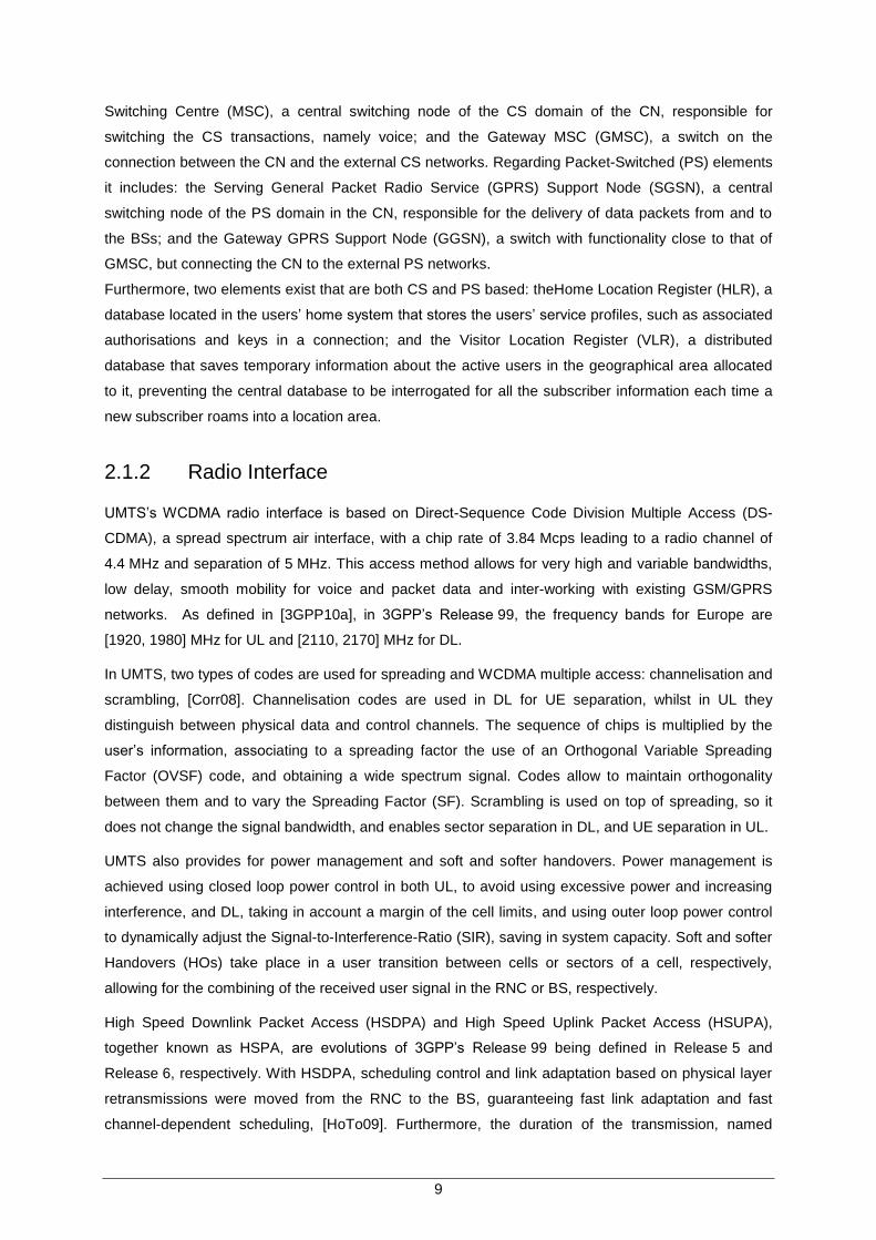
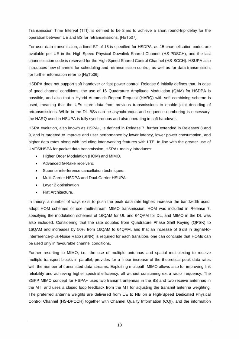
As shown in Figure 2.2, the peak bit rate with 64QAM is 21.1 Mbps, rising to 28.0 Mbps with MIMO,
whereas using 64QAM and MIMO together provide a rise from 14Mbps to 42 Mbps, [HoTo09]. The
16QAM capability in UL enables to push the peak bit rate to 11.5 Mbps, although MIMO is not used in
this link, mainly because it obliges the UE to have two power amplifiers. In DL, HOM helps to improve
the spectral efficiency because there is a limited number of orthogonal resources. The same is not
true for UL, since there is a large availability of codes. Thus, in UL, using 16QAM is a peak data
feature and not a capacity feature.
(a) DL achievable throughputs regarding HOM
schemes and MIMO configurations.
(b) UL achievable throughputs
regarding HOM schemes.
Figure 2.2. Ninetieth percentile throughput as a function of Signal-to-Noise-Ratio (SNR) in Pedestrian
A-channel (extracted from [BEGG08]) and Throughput as a function of in Pedestrian A channel
(extracted from [PWST07]).
Moreover, MTs and BSs requirements are constantly being improved to raise system performance. As
Release 6 introduced the use of receive diversity antennas (two antenna Rake receiver type 1) and
one-antenna linear equaliser (type 2), Release 7 also introduced a combination of linear equalisers
with receive diversity antenna (type 3), based on a two-antenna chip-level equaliser [HoTo07]. The
enhanced terminal receivers improve the single-user data rates and together with all other Release 7
features the cell capacity is nearly doubled compared with Release 6. Release 8 brings also an
advanced receiver, with inter-cell interference cancellation support.
Multi-Carrier HSDPA and Dual-Carrier HSUPA capabilities are introduced in HSPA+, respectively in
Release 10, [3GPP10b], and Release 9, [Seid09]. Taking the combination of two or four carriers
instead of one, Multi-Carrier HSDPA allows user data rate to be easily doubled or quadrupled mostly
when the loading is low, [JBGB09]. The BS can optimise the transmission based on CQI reporting,
similarly as in MIMO closed loop feedback for antenna weighting. As for Dual-Carrier HSUPA, a more
limited set of scenarios is defined for its use, combining two adjacent carriers for transmission of UL
physical channels and Dedicated Physical Control Channel (DPCCH) [Seid09].
Although both Dual-Carrier HSDPA and MIMO solutions are targeted to boost data rates, and can
12
provide the same peak rate of 42 Mbps with 64QAM modulation, MIMO can improve spectral
efficiency due to two antenna transmission, while the Dual-Carrier HSDPA brings some improvement
to the high loaded case with frequency domain scheduling and a larger trunking gain. Also, whilst the
Dual-Carrier solution improvement is available over the whole cell area equally, MIMO only improves
the data rates mostly close to the Node B, where dual stream transmission is feasible.
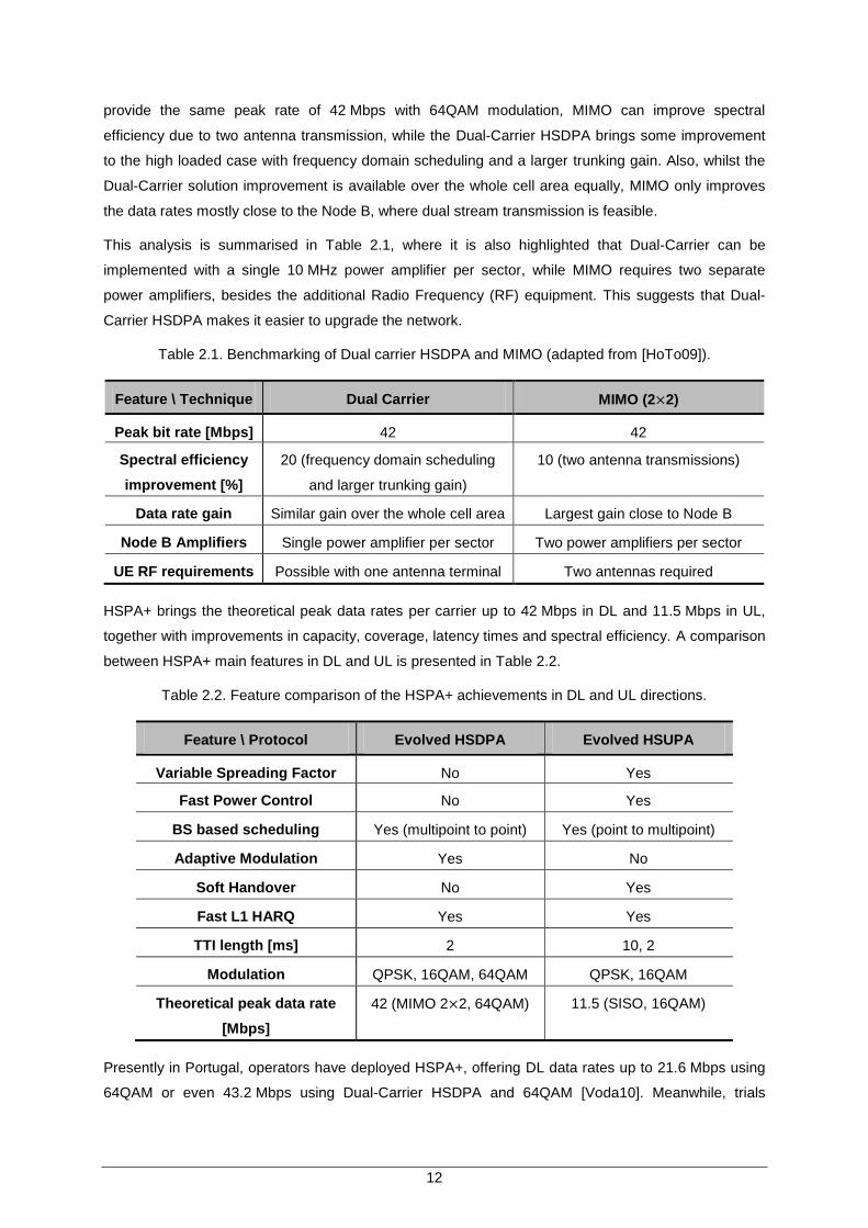
This analysis is summarised in Table 2.1, where it is also highlighted that Dual-Carrier can be
implemented with a single 10 MHz power amplifier per sector, while MIMO requires two separate
power amplifiers, besides the additional Radio Frequency (RF) equipment. This suggests that Dual-
Carrier HSDPA makes it easier to upgrade the network.
Table 2.1. Benchmarking of Dual carrier HSDPA and MIMO (adapted from [HoTo09]).
Feature \ Technique Dual Carrier MIMO (2 2)
Peak bit rate [Mbps] 42 42
Spectral efficiency
improvement [%]
20 (frequency domain scheduling
and larger trunking gain)
10 (two antenna transmissions)
Data rate gain Similar gain over the whole cell area Largest gain close to Node B
Node B Amplifiers
AAmploRadiorequir
ements Modulation
Single power amplifier per sector Two power amplifiers per sector
UE RF requirements Possible with one antenna terminal Two antennas required
HSPA+ brings the theoretical peak data rates per carrier up to 42 Mbps in DL and 11.5 Mbps in UL,
together with improvements in capacity, coverage, latency times and spectral efficiency. A comparison
between HSPA+ main features in DL and UL is presented in Table 2.2.
Table 2.2. Feature comparison of the HSPA+ achievements in DL and UL directions.
Feature \ Protocol Evolved HSDPA Evolved HSUPA
Variable Spreading Factor No Yes
Fast Power Control No Yes
BS based scheduling Yes (multipoint to point) Yes (point to multipoint)
Adaptive Modulation Yes No
Soft Handover No Yes
Fast L1 HARQ Yes Yes
TTI length [ms] 2 10, 2
Modulation QPSK, 16QAM, 64QAM QPSK, 16QAM
Theoretical peak data rate
[Mbps]
42 (MIMO 2 2, 64QAM) 11.5 (SISO, 16QAM)
Presently in Portugal, operators have deployed HSPA+, offering DL data rates up to 21.6 Mbps using
64QAM or even 43.2 Mbps using Dual-Carrier HSDPA and 64QAM [Voda10]. Meanwhile, trials
13
combining 64QAM, MIMO and Dual-Carrier HSDPA have proved to achieve 84 Mbps or even
168 Mbps for DL, just using 64QAM and Multi-Carrier combining eight carriers [Eric11].
2.1.3 Capacity and Coverage
In this thesis, the main performance parameter of interest is the data rate, associated to given
coverage and capacity. Nevertheless, interference is a primordial factor to take into account in this
analysis of the communications system.
The limiting factors on system capacity are mainly three [Corr10]: the number of available codes in DL,
the system load (interference constrains in both UL and DL), and the shared DL transmission power.
As the number of available channelisation codes is limited by SF, the number of simultaneous active
users in the cell is limited by this number. The maximum value for SF is limited to ensure a minimum
Quality of Service (QoS), whereas high SF values would allow unbearable interference levels. In
practice, for the total number of available codes in HSDPA, users would be required to be very near
the BS and in perfect channel conditions, and so this does not represent a real limit.
On the other hand, the trade-off between capacity and interference is of key importance in cellular
networks, shown by the expression for the interference margin [Corr10]:
(2.1) (2.
1) where:
: load factor, assuming values in [0,1].
The load factor depends on the services, being distinct for UL and DL due to the traffic asymmetry
between them and the different transmission powers that characterise each transmitter. The more load
is allowed in the system, the larger is the interference margin needed, and the smaller is the coverage
area. For coverage-limited cases a smaller interference margin is suggested, while in capacity-limited
cases a larger interference margin should be used. Typical values for the interference margin in the
case of coverage limitation are 1 to 3 dB, corresponding to 20-50% load, [HoTo07].
Alternatively to an interference margin, intra-cell and inter-cell interferences can be computed using
expressions (2.2) and (2.3) for the DL, and (2.4)and (2.5) for UL, [EsPe06].
(2.2) (2.
2) where:
: code orthogonality factor (typically [50, 90] %);
: total BS transmitted power;
: BS transmitted power to user ;
: pathloss from serving BS to user ;
(2.3) (2.
3)
where:
14
: number of neighbouring BSs;
: BS transmitted power;
: pathloss from BS to the user.
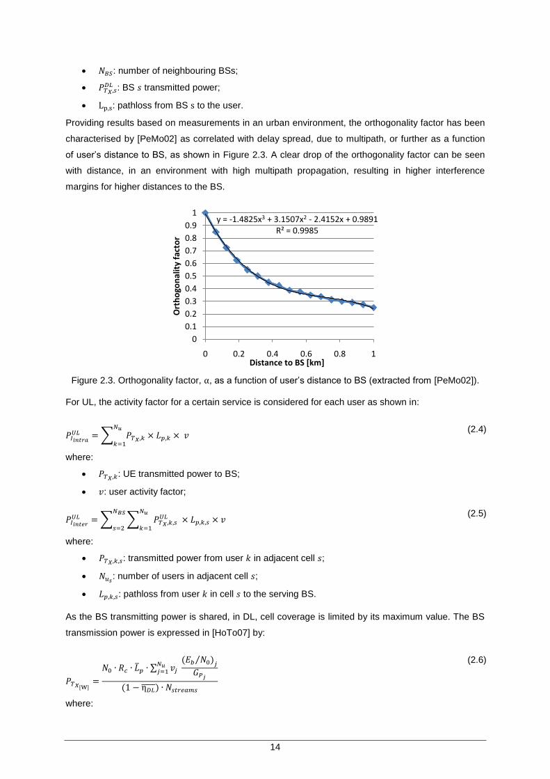
Providing results based on measurements in an urban environment, the orthogonality factor has been
characterised by [PeMo02] as correlated with delay spread, due to multipath, or further as a function
of user‟s distance to BS, as shown in Figure 2.3. A clear drop of the orthogonality factor can be seen
with distance, in an environment with high multipath propagation, resulting in higher interference
margins for higher distances to the BS.
Figure 2.3. Orthogonality factor, , as a function of user‟s distance to BS (extracted from [PeMo02]).
For UL, the activity factor for a certain service is considered for each user as shown in:
(2.4) (2.
4)
where:
: UE transmitted power to BS;
: user activity factor;
(2.5) (2.
5)
where:
: transmitted power from user in adjacent cell ;
: number of users in adjacent cell ;
: pathloss from user in cell to the serving BS.
As the BS transmitting power is shared, in DL, cell coverage is limited by its maximum value. The BS
transmission power is expressed in [HoTo07] by:
(2.6) (2.
6)
where:
y = -1.4825x3 + 3.1507x2 - 2.4152x + 0.9891R² = 0.9985
0
0.1
0.2
0.3
0.4
0.5
0.6
0.7
0.8
0.9
1
0 0.2 0.4 0.6 0.8 1
Ort
ho
gon
alit
y fa
cto
r
Distance to BS [km]
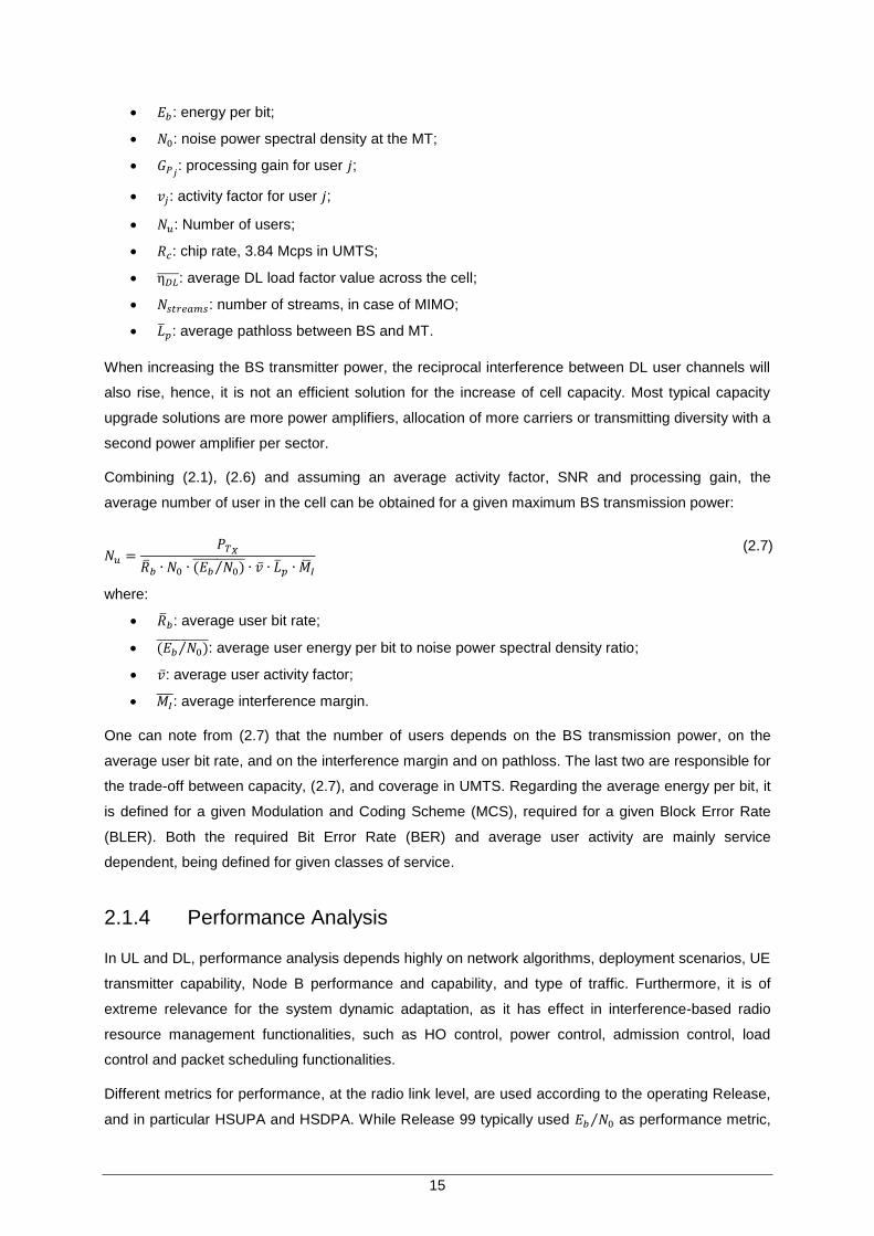
15
: energy per bit;
: noise power spectral density at the MT;
: processing gain for user ;
: activity factor for user ;
: Number of users;
: chip rate, 3.84 Mcps in UMTS;
: average DL load factor value across the cell;
: number of streams, in case of MIMO;
: average pathloss between BS and MT.
When increasing the BS transmitter power, the reciprocal interference between DL user channels will
also rise, hence, it is not an efficient solution for the increase of cell capacity. Most typical capacity
upgrade solutions are more power amplifiers, allocation of more carriers or transmitting diversity with a
second power amplifier per sector.
Combining (2.1), (2.6) and assuming an average activity factor, SNR and processing gain, the
average number of user in the cell can be obtained for a given maximum BS transmission power:
(2.7) (
2.
7)
where:
: average user bit rate;
: average user energy per bit to noise power spectral density ratio;
: average user activity factor;
: average interference margin.
One can note from (2.7) that the number of users depends on the BS transmission power, on the
average user bit rate, and on the interference margin and on pathloss. The last two are responsible for
the trade-off between capacity, (2.7), and coverage in UMTS. Regarding the average energy per bit, it
is defined for a given Modulation and Coding Scheme (MCS), required for a given Block Error Rate
(BLER). Both the required Bit Error Rate (BER) and average user activity are mainly service
dependent, being defined for given classes of service.
2.1.4 Performance Analysis
In UL and DL, performance analysis depends highly on network algorithms, deployment scenarios, UE
transmitter capability, Node B performance and capability, and type of traffic. Furthermore, it is of
extreme relevance for the system dynamic adaptation, as it has effect in interference-based radio
resource management functionalities, such as HO control, power control, admission control, load
control and packet scheduling functionalities.
Different metrics for performance, at the radio link level, are used according to the operating Release,
and in particular HSUPA and HSDPA. While Release 99 typically used as performance metric,
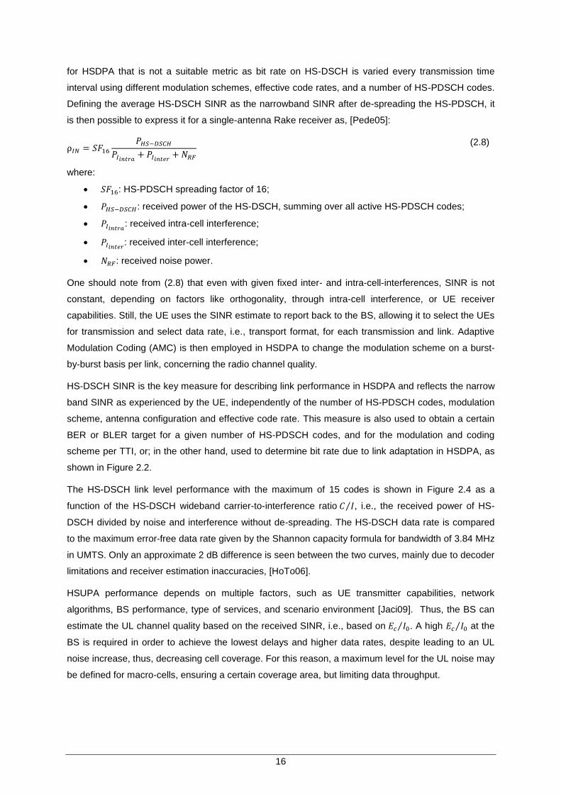
16
for HSDPA that is not a suitable metric as bit rate on HS-DSCH is varied every transmission time
interval using different modulation schemes, effective code rates, and a number of HS-PDSCH codes.
Defining the average HS-DSCH SINR as the narrowband SINR after de-spreading the HS-PDSCH, it
is then possible to express it for a single-antenna Rake receiver as, [Pede05]:
(2.8) (
2.8)
where:
: HS-PDSCH spreading factor of 16;
: received power of the HS-DSCH, summing over all active HS-PDSCH codes;
: received intra-cell interference;
: received inter-cell interference;
: received noise power.
One should note from (2.8) that even with given fixed inter- and intra-cell-interferences, SINR is not
constant, depending on factors like orthogonality, through intra-cell interference, or UE receiver
capabilities. Still, the UE uses the SINR estimate to report back to the BS, allowing it to select the UEs
for transmission and select data rate, i.e., transport format, for each transmission and link. Adaptive
Modulation Coding (AMC) is then employed in HSDPA to change the modulation scheme on a burst-
by-burst basis per link, concerning the radio channel quality.
HS-DSCH SINR is the key measure for describing link performance in HSDPA and reflects the narrow
band SINR as experienced by the UE, independently of the number of HS-PDSCH codes, modulation
scheme, antenna configuration and effective code rate. This measure is also used to obtain a certain
BER or BLER target for a given number of HS-PDSCH codes, and for the modulation and coding
scheme per TTI, or; in the other hand, used to determine bit rate due to link adaptation in HSDPA, as
shown in Figure 2.2.
The HS-DSCH link level performance with the maximum of 15 codes is shown in Figure 2.4 as a
function of the HS-DSCH wideband carrier-to-interference ratio , i.e., the received power of HS-
DSCH divided by noise and interference without de-spreading. The HS-DSCH data rate is compared
to the maximum error-free data rate given by the Shannon capacity formula for bandwidth of 3.84 MHz
in UMTS. Only an approximate 2 dB difference is seen between the two curves, mainly due to decoder
limitations and receiver estimation inaccuracies, [HoTo06].
HSUPA performance depends on multiple factors, such as UE transmitter capabilities, network
algorithms, BS performance, type of services, and scenario environment [Jaci09]. Thus, the BS can
estimate the UL channel quality based on the received SINR, i.e., based on . A high at the
BS is required in order to achieve the lowest delays and higher data rates, despite leading to an UL
noise increase, thus, decreasing cell coverage. For this reason, a maximum level for the UL noise may
be defined for macro-cells, ensuring a certain coverage area, but limiting data throughput.
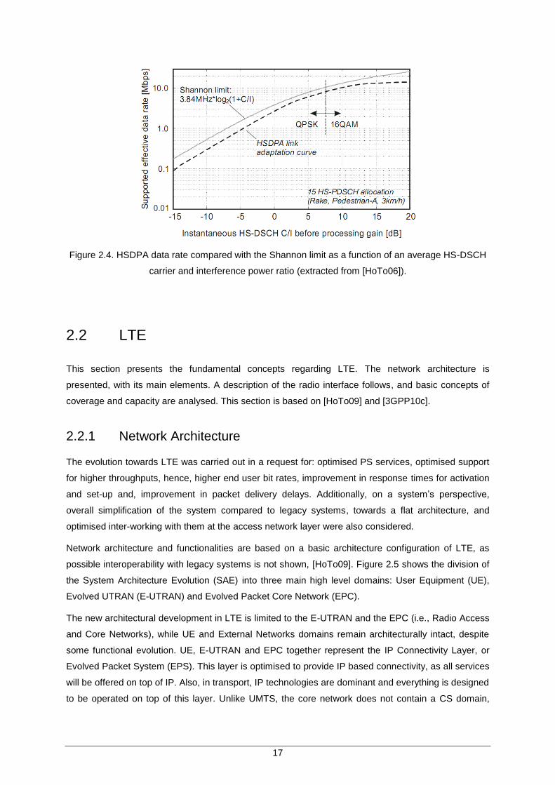
17
Figure 2.4. HSDPA data rate compared with the Shannon limit as a function of an average HS-DSCH
carrier and interference power ratio (extracted from [HoTo06]).
2.2 LTE
This section presents the fundamental concepts regarding LTE. The network architecture is
presented, with its main elements. A description of the radio interface follows, and basic concepts of
coverage and capacity are analysed. This section is based on [HoTo09] and [3GPP10c].
2.2.1 Network Architecture
The evolution towards LTE was carried out in a request for: optimised PS services, optimised support
for higher throughputs, hence, higher end user bit rates, improvement in response times for activation
and set-up and, improvement in packet delivery delays. Additionally, on a system‟s perspective,
overall simplification of the system compared to legacy systems, towards a flat architecture, and
optimised inter-working with them at the access network layer were also considered.
Network architecture and functionalities are based on a basic architecture configuration of LTE, as
possible interoperability with legacy systems is not shown, [HoTo09]. Figure 2.5 shows the division of
the System Architecture Evolution (SAE) into three main high level domains: User Equipment (UE),
Evolved UTRAN (E-UTRAN) and Evolved Packet Core Network (EPC).
The new architectural development in LTE is limited to the E-UTRAN and the EPC (i.e., Radio Access
and Core Networks), while UE and External Networks domains remain architecturally intact, despite
some functional evolution. UE, E-UTRAN and EPC together represent the IP Connectivity Layer, or
Evolved Packet System (EPS). This layer is optimised to provide IP based connectivity, as all services
will be offered on top of IP. Also, in transport, IP technologies are dominant and everything is designed
to be operated on top of this layer. Unlike UMTS, the core network does not contain a CS domain,
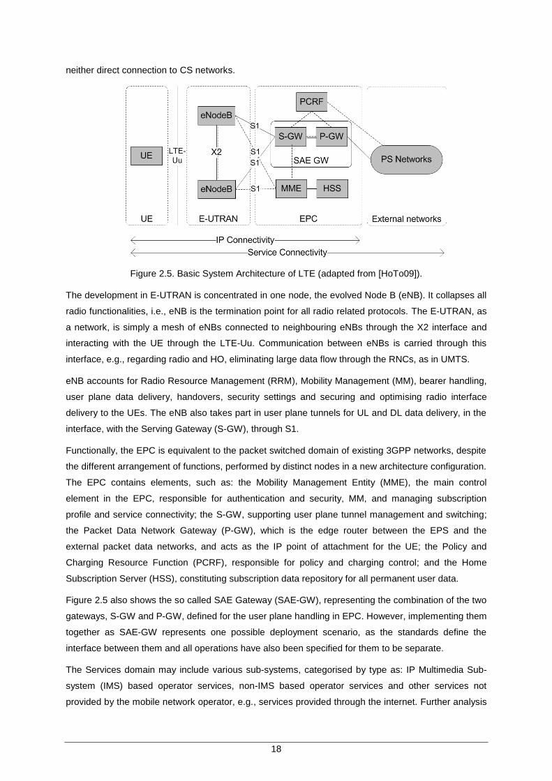
18
neither direct connection to CS networks.
Figure 2.5. Basic System Architecture of LTE (adapted from [HoTo09]).
The development in E-UTRAN is concentrated in one node, the evolved Node B (eNB). It collapses all
radio functionalities, i.e., eNB is the termination point for all radio related protocols. The E-UTRAN, as
a network, is simply a mesh of eNBs connected to neighbouring eNBs through the X2 interface and
interacting with the UE through the LTE-Uu. Communication between eNBs is carried through this
interface, e.g., regarding radio and HO, eliminating large data flow through the RNCs, as in UMTS.
eNB accounts for Radio Resource Management (RRM), Mobility Management (MM), bearer handling,
user plane data delivery, handovers, security settings and securing and optimising radio interface
delivery to the UEs. The eNB also takes part in user plane tunnels for UL and DL data delivery, in the
interface, with the Serving Gateway (S-GW), through S1.
Functionally, the EPC is equivalent to the packet switched domain of existing 3GPP networks, despite
the different arrangement of functions, performed by distinct nodes in a new architecture configuration.
The EPC contains elements, such as: the Mobility Management Entity (MME), the main control
element in the EPC, responsible for authentication and security, MM, and managing subscription
profile and service connectivity; the S-GW, supporting user plane tunnel management and switching;
the Packet Data Network Gateway (P-GW), which is the edge router between the EPS and the
external packet data networks, and acts as the IP point of attachment for the UE; the Policy and
Charging Resource Function (PCRF), responsible for policy and charging control; and the Home
Subscription Server (HSS), constituting subscription data repository for all permanent user data.
Figure 2.5 also shows the so called SAE Gateway (SAE-GW), representing the combination of the two
gateways, S-GW and P-GW, defined for the user plane handling in EPC. However, implementing them
together as SAE-GW represents one possible deployment scenario, as the standards define the
interface between them and all operations have also been specified for them to be separate.
The Services domain may include various sub-systems, categorised by type as: IP Multimedia Sub-
system (IMS) based operator services, non-IMS based operator services and other services not
provided by the mobile network operator, e.g., services provided through the internet. Further analysis
19
about service level systems is out of the scope of this thesis, but particularly for IMS, the preferred
service machinery for LTE/SAE, the interested reader should refer to [HoTo09] and [PoMa09].
2.2.2 Radio Interface
For LTE, two multiple access techniques are employed: Orthogonal Frequency Division Multiple
Access (OFDMA) for DL and Single Carrier Frequency Division Multiple Access (SC-FDMA) with
Cyclic Prefix (CP) for UL. OFDMA allows the access of multiple users on the available bandwidth by
dynamically assigning each user to a specific time-frequency resource. Using SC-FDMA, the same
technique is employed, but with the distinguishing feature that it leads to a single-carrier transmit
signal, while OFDMA is a multi-carrier transmission scheme. LTE supports both Frequency Division
Duplexing (FDD) and Time Division Duplexing (TDD), although only FDD is addressed in this thesis
due to its wide adoption in the majority of European networks. According to the specifications, there
are 17 frequency FDD bands and 8 TDD bands of LTE spectrum allocated [3GPP10d]. In Europe, and
particularly in Portugal, regulation has been issued under public consultation for the auction of the
800 MHz, 900 MHz, 1800 MHz, 2.1 GHz and 2.6 GHz frequency bands [ANAC11].
The difference in the access techniques chosen for DL and UL is mainly related with the
characteristics of better efficiency power and lower Peak-to-Average-power-Ratio (PAR). Compared to
OFDM, SC-FDMA in UL ultimately maximises battery life for the MT as a reduction of 2 dB in PAR is
achieved comparing to OFDMA, [Zeme08]. Additionally, the CP avoids Inter-Symbol Interference (ISI),
and can be chosen to be normal or extended so to be slightly longer than the longest delay spread in
the radio channel. This approach allows for simple frequency-domain processing, such as channel
estimation and equalisation, with advantages both in UL and DL.
Channel estimation is necessary in LTE, both in UL and DL, as the receiver still has to deal with the
channel impact for the individual subcarriers that have experienced frequency dependent phase and
amplitude errors. The estimation is done through the use of pilot or reference symbols, which facilitate
coherent channel estimation and allow reverting channel impact for each subcarrier, e.g., by using a
frequency domain equaliser.
In DL, it is allowed for scalable carrier bandwidths, from 1.4 up to 20 MHz, with subcarrier spacing of
15 kHz [3GPP10c]. In LTE, the concept of a Resource Block (RB) is used, which is a block of 12
subcarriers in one slot, i.e., 180 kHz in the frequency domain. Each time slot is 0.5 ms long, a group of
2 slots is a sub-frame of 1 ms (or the TTI) and each frame is 10 ms. Furthermore, a transport block is
a group of resource blocks with a common modulation or coding. The physical interface is a transport
block, which corresponds to the data carried in a period of time allocated to a particular UE. Multiple
UEs can be serviced on DL at any particular time in one transport block.
The time domain structure of the frame used in LTE is, in most respects, the same for FDD and TDD,
Figure 2.6. Some differences exist between the two duplex modes, most notably the presence of a
special sub-frame in case of TDD. Nevertheless, LTE‟s physical layer, like the general system, is
designed for maximum efficiency of the packet-based transmission, and for this reason, there are only
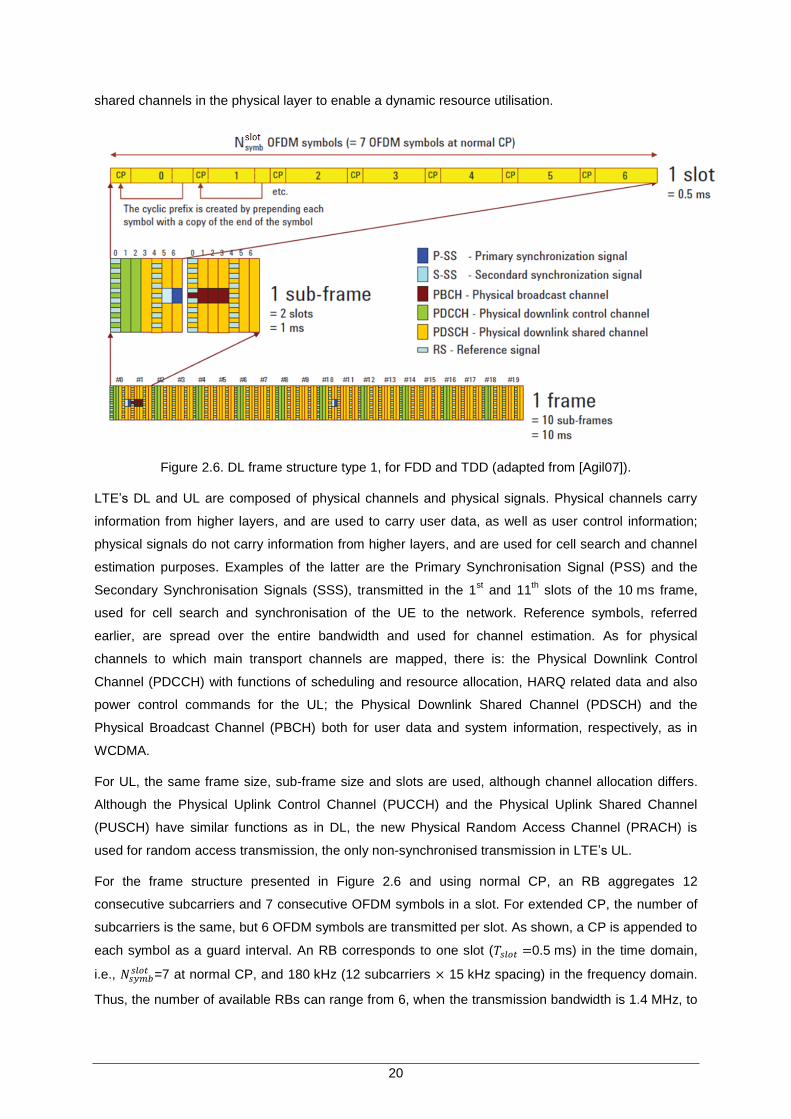
20
shared channels in the physical layer to enable a dynamic resource utilisation.
Figure 2.6. DL frame structure type 1, for FDD and TDD (adapted from [Agil07]).
LTE‟s DL and UL are composed of physical channels and physical signals. Physical channels carry
information from higher layers, and are used to carry user data, as well as user control information;
physical signals do not carry information from higher layers, and are used for cell search and channel
estimation purposes. Examples of the latter are the Primary Synchronisation Signal (PSS) and the
Secondary Synchronisation Signals (SSS), transmitted in the 1st and 11
th slots of the 10 ms frame,
used for cell search and synchronisation of the UE to the network. Reference symbols, referred
earlier, are spread over the entire bandwidth and used for channel estimation. As for physical
channels to which main transport channels are mapped, there is: the Physical Downlink Control
Channel (PDCCH) with functions of scheduling and resource allocation, HARQ related data and also
power control commands for the UL; the Physical Downlink Shared Channel (PDSCH) and the
Physical Broadcast Channel (PBCH) both for user data and system information, respectively, as in
WCDMA.
For UL, the same frame size, sub-frame size and slots are used, although channel allocation differs.
Although the Physical Uplink Control Channel (PUCCH) and the Physical Uplink Shared Channel
(PUSCH) have similar functions as in DL, the new Physical Random Access Channel (PRACH) is
used for random access transmission, the only non-synchronised transmission in LTE‟s UL.
For the frame structure presented in Figure 2.6 and using normal CP, an RB aggregates 12
consecutive subcarriers and 7 consecutive OFDM symbols in a slot. For extended CP, the number of
subcarriers is the same, but 6 OFDM symbols are transmitted per slot. As shown, a CP is appended to
each symbol as a guard interval. An RB corresponds to one slot ( 0.5 ms) in the time domain,
i.e., =7 at normal CP, and 180 kHz (12 subcarriers 15 kHz spacing) in the frequency domain.
Thus, the number of available RBs can range from 6, when the transmission bandwidth is 1.4 MHz, to
21
100, when it is 20 MHz.
For LTE, power control only exists for UL, and does not control absolute power, but rather the power
spectral density, for a particular device. Furthermore, the use of orthogonal resources in UL facilitates
the use of a slower rate for power control, unlike WCDMA systems where fast power control is
required. The key motivation in LTE is, hence, to reduce terminal power consumption and also to
avoid overly large dynamic range in the eNB receiver, rather than to mitigate interference.
Besides optimisation in time and frequency domains, antenna optimisation through MIMO is the key
enabler of a high data rate in LTE. For this reason, plain SISO transmission is not supported as UEs
are required to have at least two receiving antennas and the SIMO case constitutes then the simplest
scheme. Further information on MIMO for LTE is presented in Annex D.
2.2.3 Capacity and Coverage
Theoretical bit rates, can be obtained for DL using:
(2.9) (
2.9)
where:
: number of subcarriers per resource block (assumed 12 for 15 kHz subcarrier spacing);
: number of user resource blocks;
: order of the modulation considered;
: number of symbols per sub-frame (14 symbols for normal CP or 12 for extended CP);
: number of streams, in case of MIMO;
: sub-frame period, 1 ms.
As seen in (2.9), end-user throughput depends on parameters like modulation and MIMO
configurations used, directly related with channel conditions, CP size used, and number of resource
blocks allocated for a certain user. However, note also that user throughput depends additionally on
the overhead amount due to synchronisation and reference signals as well as control channels.
Moreover given the dynamic allocation of time-frequency resources in the eNB, the multi-user
scheduling strategies are directly related to user data rates and user capacity, both at the cellular and
system level. Main capacity limiting factors include the number of resource blocks, scheduler
implementation efficiency, inter-cell interference, MIMO, and supported modulation and coding
schemes.
To maximise service delivery for the user, a variety of resource scheduling algorithms may be applied
by the eNB, depending on the optimisation criteria required, searching for a fair balance between
throughput maximisation for delay-tolerant applications against QoS for delay applications. The
prioritisation of data will typically consider the corresponding traffic classes, as shown in [HoTo09]. For
this, multi-user diversity is an important factor, especially if the user density is high, in which case the
multi-user diversity gain will enable the scheduler to achieve a high capacity, even with tight delay
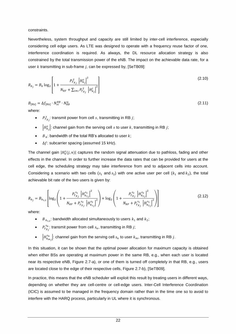
22
constraints.
Nevertheless, system throughput and capacity are still limited by inter-cell interference, especially
considering cell edge users. As LTE was designed to operate with a frequency reuse factor of one,
interference coordination is required. As always, the DL resource allocation strategy is also
constrained by the total transmission power of the eNB. The impact on the achievable data rate, for a
user transmitting in sub-frame , can be expressed by, [SeTB09]:
(2.10) (2.13)
(2.11) (2.14)
where:
: transmit power from cell , transmitting in RB ;
: channel gain from the serving cell to user , transmitting in RB ;
: bandwidth of the total RB‟s allocated to user ;
: subcarrier spacing (assumed 15 kHz).
The channel gain captures the random signal attenuation due to pathloss, fading and other
effects in the channel. In order to further increase the data rates that can be provided for users at the
cell edge, the scheduling strategy may take interference from and to adjacent cells into account.
Considering a scenario with two cells ( and ) with one active user per cell ( and ), the total
achievable bit rate of the two users is given by:
(2.12) (2.15)
where:
: bandwidth allocated simultaneously to users and ;
: transmit power from cell , transmitting in RB ;
: channel gain from the serving cell to user , transmitting in RB .
In this situation, it can be shown that the optimal power allocation for maximum capacity is obtained
when either BSs are operating at maximum power in the same RB, e.g., when each user is located
near its respective eNB, Figure 2.7-a), or one of them is turned off completely in that RB, e.g., users
are located close to the edge of their respective cells, Figure 2.7-b), [SeTB09].
In practice, this means that the eNB scheduler will exploit this result by treating users in different ways,
depending on whether they are cell-centre or cell-edge users. Inter-Cell Interference Coordination
(ICIC) is assumed to be managed in the frequency domain rather than in the time one so to avoid to
interfere with the HARQ process, particularly in UL where it is synchronous.
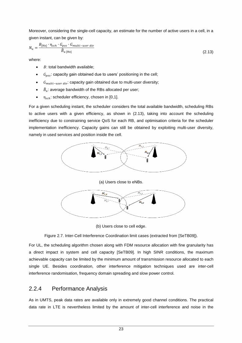
23
Moreover, considering the single-cell capacity, an estimate for the number of active users in a cell, in a
given instant, can be given by:
(2.13) (2.13)
where:
: total bandwidth available;
: capacity gain obtained due to users‟ positioning in the cell;
: capacity gain obtained due to multi-user diversity;
: average bandwidth of the RBs allocated per user;
: scheduler efficiency, chosen in [0,1].
For a given scheduling instant, the scheduler considers the total available bandwidth, scheduling RBs
to active users with a given efficiency, as shown in (2.13), taking into account the scheduling
inefficiency due to constraining service QoS for each RB, and optimisation criteria for the scheduler
implementation inefficiency. Capacity gains can still be obtained by exploiting multi-user diversity,
namely in used services and position inside the cell.
(a) Users close to eNBs.
(b) Users close to cell edge.
Figure 2.7. Inter-Cell Interference Coordination limit cases (extracted from [SeTB09]).
For UL, the scheduling algorithm chosen along with FDM resource allocation with fine granularity has
a direct impact in system and cell capacity [SeTB09]. In high SINR conditions, the maximum
achievable capacity can be limited by the minimum amount of transmission resource allocated to each
single UE. Besides coordination, other interference mitigation techniques used are inter-cell
interference randomisation, frequency domain spreading and slow power control.
2.2.4 Performance Analysis
As in UMTS, peak data rates are available only in extremely good channel conditions. The practical
data rate in LTE is nevertheless limited by the amount of inter-cell interference and noise in the
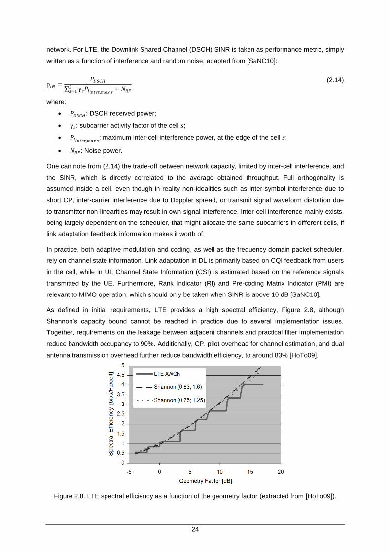
24
network. For LTE, the Downlink Shared Channel (DSCH) SINR is taken as performance metric, simply
written as a function of interference and random noise, adapted from [SaNC10]:
(2.14) (
2.14)
where:
: DSCH received power;
: subcarrier activity factor of the cell ;
: maximum inter-cell interference power, at the edge of the cell ;
: Noise power.
One can note from (2.14) the trade-off between network capacity, limited by inter-cell interference, and
the SINR, which is directly correlated to the average obtained throughput. Full orthogonality is
assumed inside a cell, even though in reality non-idealities such as inter-symbol interference due to
short CP, inter-carrier interference due to Doppler spread, or transmit signal waveform distortion due
to transmitter non-linearities may result in own-signal interference. Inter-cell interference mainly exists,
being largely dependent on the scheduler, that might allocate the same subcarriers in different cells, if
link adaptation feedback information makes it worth of.
In practice, both adaptive modulation and coding, as well as the frequency domain packet scheduler,
rely on channel state information. Link adaptation in DL is primarily based on CQI feedback from users
in the cell, while in UL Channel State Information (CSI) is estimated based on the reference signals
transmitted by the UE. Furthermore, Rank Indicator (RI) and Pre-coding Matrix Indicator (PMI) are
relevant to MIMO operation, which should only be taken when SINR is above 10 dB [SaNC10].
As defined in initial requirements, LTE provides a high spectral efficiency, Figure 2.8, although
Shannon‟s capacity bound cannot be reached in practice due to several implementation issues.
Together, requirements on the leakage between adjacent channels and practical filter implementation
reduce bandwidth occupancy to 90%. Additionally, CP, pilot overhead for channel estimation, and dual
antenna transmission overhead further reduce bandwidth efficiency, to around 83% [HoTo09].
Figure 2.8. LTE spectral efficiency as a function of the geometry factor (extracted from [HoTo09]).
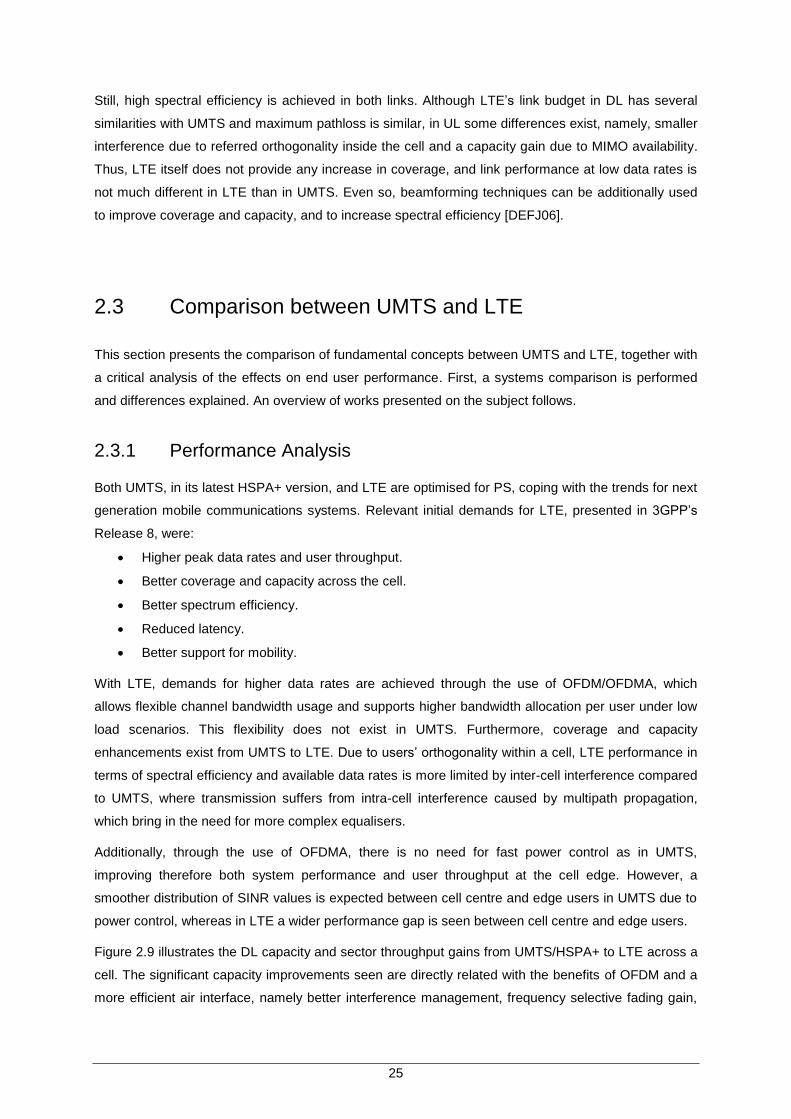
25
Still, high spectral efficiency is achieved in both links. Although LTE‟s link budget in DL has several
similarities with UMTS and maximum pathloss is similar, in UL some differences exist, namely, smaller
interference due to referred orthogonality inside the cell and a capacity gain due to MIMO availability.
Thus, LTE itself does not provide any increase in coverage, and link performance at low data rates is
not much different in LTE than in UMTS. Even so, beamforming techniques can be additionally used
to improve coverage and capacity, and to increase spectral efficiency [DEFJ06].
2.3 Comparison between UMTS and LTE
This section presents the comparison of fundamental concepts between UMTS and LTE, together with
a critical analysis of the effects on end user performance. First, a systems comparison is performed
and differences explained. An overview of works presented on the subject follows.
2.3.1 Performance Analysis
Both UMTS, in its latest HSPA+ version, and LTE are optimised for PS, coping with the trends for next
generation mobile communications systems. Relevant initial demands for LTE, presented in 3GPP‟s
Release 8, were:
Higher peak data rates and user throughput.
Better coverage and capacity across the cell.
Better spectrum efficiency.
Reduced latency.
Better support for mobility.
With LTE, demands for higher data rates are achieved through the use of OFDM/OFDMA, which
allows flexible channel bandwidth usage and supports higher bandwidth allocation per user under low
load scenarios. This flexibility does not exist in UMTS. Furthermore, coverage and capacity
enhancements exist from UMTS to LTE. Due to users‟ orthogonality within a cell, LTE performance in
terms of spectral efficiency and available data rates is more limited by inter-cell interference compared
to UMTS, where transmission suffers from intra-cell interference caused by multipath propagation,
which bring in the need for more complex equalisers.
Additionally, through the use of OFDMA, there is no need for fast power control as in UMTS,
improving therefore both system performance and user throughput at the cell edge. However, a
smoother distribution of SINR values is expected between cell centre and edge users in UMTS due to
power control, whereas in LTE a wider performance gap is seen between cell centre and edge users.
Figure 2.9 illustrates the DL capacity and sector throughput gains from UMTS/HSPA+ to LTE across a
cell. The significant capacity improvements seen are directly related with the benefits of OFDM and a
more efficient air interface, namely better interference management, frequency selective fading gain,
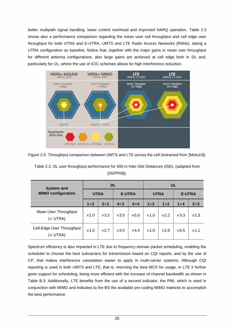
26
better multipath signal handling, lower control overhead and improved HARQ operation. Table 2.3
shows also a performance comparison regarding the mean user cell throughput and cell edge user
throughput for both UTRA and E-UTRA, UMTS and LTE Radio Access Networks (RANs), taking a
UTRA configuration as baseline. Notice that, together with the major gains in mean user throughput
for different antenna configurations, also large gains are achieved at cell edge both in DL and,
particularly for UL, where the use of ICIC schemes allows for high interference reduction.
Figure 2.9. Throughput comparison between UMTS and LTE across the cell (extracted from [Moto10]).
Table 2.3. DL user throughput performance for 500 m Inter-Site Distances (ISD), (adapted from
[3GPP09]).
System and
MIMO configuration
DL UL
UTRA E-UTRA UTRA E-UTRA
1 2 2 2 4 2 4 4 1 2 1 2 1 4 2 2
Mean User Throughput
( UTRA) 1.0 3.2 3.5 5.0 1.0 2.2 3.3 2.3
Cell-Edge User Throughput
( UTRA) 1.0 2.7 3.0 4.4 1.0 2.5 5.5 1.1
Spectrum efficiency is also impacted in LTE due to frequency domain packet scheduling, enabling the
scheduler to choose the best subcarriers for transmission based on CQI reports, and by the use of
CP, that makes interference cancelation easier to apply in multi-carrier systems. Although CQI
reporting is used in both UMTS and LTE, that is, returning the best MCS for usage, in LTE it further
gives support for scheduling, being more efficient with the increase of channel bandwidth as shown in
Table B.3. Additionally, LTE benefits from the use of a second indicator, the PMI, which is used in
conjunction with MIMO and indicates to the BS the available pre-coding MIMO matrices to accomplish
the best performance.
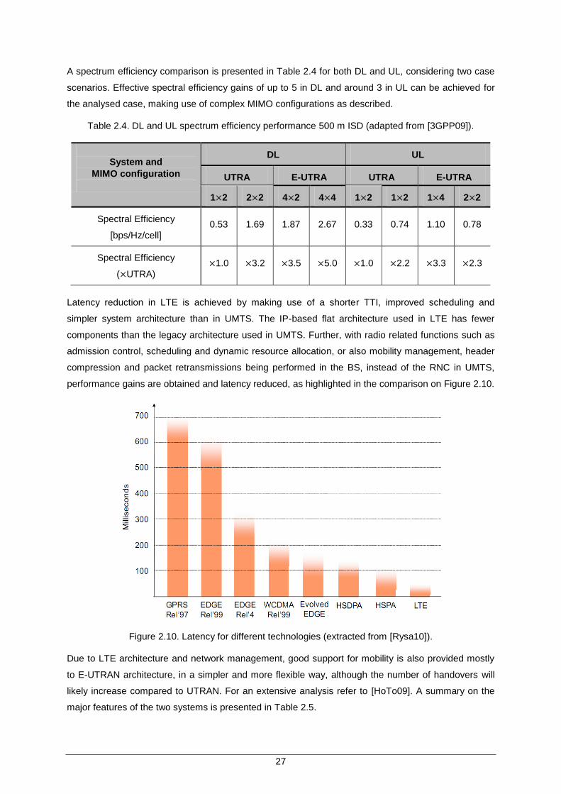
27
A spectrum efficiency comparison is presented in Table 2.4 for both DL and UL, considering two case
scenarios. Effective spectral efficiency gains of up to 5 in DL and around 3 in UL can be achieved for
the analysed case, making use of complex MIMO configurations as described.
Table 2.4. DL and UL spectrum efficiency performance 500 m ISD (adapted from [3GPP09]).
System and
MIMO configuration
DL UL
UTRA E-UTRA UTRA E-UTRA
1 2 2 2 4 2 4 4 1 2 1 2 1 4 2 2
Spectral Efficiency
[bps/Hz/cell] 0.53 1.69 1.87 2.67 0.33 0.74 1.10 0.78
Spectral Efficiency
( UTRA) 1.0 3.2 3.5 5.0 1.0 2.2 3.3 2.3
Latency reduction in LTE is achieved by making use of a shorter TTI, improved scheduling and
simpler system architecture than in UMTS. The IP-based flat architecture used in LTE has fewer
components than the legacy architecture used in UMTS. Further, with radio related functions such as
admission control, scheduling and dynamic resource allocation, or also mobility management, header
compression and packet retransmissions being performed in the BS, instead of the RNC in UMTS,
performance gains are obtained and latency reduced, as highlighted in the comparison on Figure 2.10.
Figure 2.10. Latency for different technologies (extracted from [Rysa10]).
Due to LTE architecture and network management, good support for mobility is also provided mostly
to E-UTRAN architecture, in a simpler and more flexible way, although the number of handovers will
likely increase compared to UTRAN. For an extensive analysis refer to [HoTo09]. A summary on the
major features of the two systems is presented in Table 2.5.
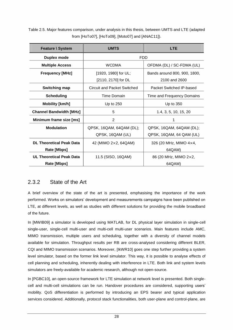
28
Table 2.5. Major features comparison, under analysis in this thesis, between UMTS and LTE (adapted
from [HoTo07], [HoTo09], [Moto07] and [ANAC11]).
Feature \ System UMTS LTE
Duplex mode FDD
Multiple Access WCDMA OFDMA (DL) / SC-FDMA (UL)
Frequency [MHz] [1920, 1980] for UL;
[2110, 2170] for DL
Bands around 800, 900, 1800,
2100 and 2600
Switching map Circuit and Packet Switched Packet Switched IP-based
Scheduling Time Domain Time and Frequency Domains
Mobility [km/h] Up to 250 Up to 350
Channel Bandwidth [MHz] 5 1.4, 3, 5, 10, 15, 20
Minimum frame size [ms] 2 1
Modulation QPSK, 16QAM, 64QAM (DL);
QPSK, 16QAM (UL)
QPSK, 16QAM, 64QAM (DL);
QPSK, 16QAM, 64 QAM (UL)
DL Theoretical Peak Data
Rate [Mbps]
42 (MIMO 2 2, 64QAM) 326 (20 MHz, MIMO 4 4,
64QAM)
UL Theoretical Peak Data
Rate [Mbps]
11.5 (SISO, 16QAM) 86 (20 MHz, MIMO 2 2,
64QAM)
2.3.2 State of the Art
A brief overview of the state of the art is presented, emphasising the importance of the work
performed. Works on simulators‟ development and measurements campaigns have been published on
LTE, at different levels, as well as studies with different solutions for providing the mobile broadband
of the future.
In [MWIB09] a simulator is developed using MATLAB, for DL physical layer simulation in single-cell
single-user, single-cell multi-user and multi-cell multi-user scenarios. Main features include AMC,
MIMO transmission, multiple users and scheduling, together with a diversity of channel models
available for simulation. Throughput results per RB are cross-analysed considering different BLER,
CQI and MIMO transmission scenarios. Moreover, [IkWR10] goes one step further providing a system
level simulator, based on the former link level simulator. This way, it is possible to analyse effects of
cell planning and scheduling, inherently dealing with interference in LTE. Both link and system levels
simulators are freely-available for academic research, although not open-source.
In [PGBC10], an open-source framework for LTE simulation at network level is presented. Both single-
cell and multi-cell simulations can be run. Handover procedures are considered, supporting users‟
mobility. QoS differentiation is performed by introducing an EPS bearer and typical application
services considered. Additionally, protocol stack functionalities, both user-plane and control-plane, are
29
considered for MAC, RLC, Packet Data Convergence Protocol (PDCP) and IP layers. Remarkable
resource management features, namely bandwidth management, frequency reuse scheme selection,
frame structure selection and radio resource scheduling are available for simulation.
Additionally, manufactures have led trial tests on future LTE system. [Eric08] shows LTE performance
results on the field. MIMO gains are measured in realistic environments and good system performance
verified for varying bandwidth, antenna configuration, channel and service, using two kinds of
terminals. Increases of 50% and 113% at the median are further measured in [Eric10] at cell centre
and cell edge, from 2 2 MIMO to 4 4 MIMO. [Noki09] also shows similar measurements‟ results over
mobility scenarios, terminal category, antenna configuration, modulation scheme, layer-1 and IP layer
and QoS bearer.
Focusing on LTE specific features, [Duar08] extensively analyses different technologies in UMTS
evolution to LTE, whereas [Jaci09] studied both systems over a network perspective, evaluating
effects when varying bandwidth, frequency band, service user profiles and the use of adaptive
modulation. In the latter, higher average network throughput of 13.5 Mbps and average ratio of served
users of 72% are presented, compared to 9.8 Mbps and 66% in UMTS/HSPA+.
In an alternative approach, some studies have been conducted using a combination of different
technologies including or excluding LTE, as the next mobile communications system. Whereas
[Perg08] studies the deployment of Worldwide Interoperability for Microwave Access (WiMAX) as an
alternative to UMTS in the specific scenario of Mobility, [VeCo11] goes ahead in presenting a solution
for the resource management in a heterogeneous network solution using UMTS, Wi-Fi and WiMAX.
Despite the rich research on the subject, space still exists for specific analyses. While simulation
provides for an accurate analysis regarding LTE‟s system features, in practice either due to varying
implementation decisions taken by the equipment‟s manufacturer, varying system planning and
consequent deployment, different environment characteristics, or simply to practical matters on users‟
behaviour and usage profile, among other factors, obtained results differ drastically. Although provided
with adequate planning tools, operators still have the need for studies of more practical value.
On the other hand, manufacturer‟s measurements vary deeply with implementation aspects, left
unspecified by 3GPP and also with the study conditions. Additionally, manufacturer‟s in general have
the obvious interest of providing for the best results on the gains with the new technology, pushing the
migration into the next generation systems. In this sense, trial deployments are conceded to operators
in lab environment, with the objective of showing the best of all possible results.
Thus, by presenting a capacity and coverage study based on both simulation and measurements in a
live LTE network, this thesis is expected to be of great practical value for operators and manufacturers
in general. Furthermore, as a new model is developed for LTE simulation, embedded in LTE
measurements results, the work contributes for research on the topic inside the academic community.
Additionally, by comparing theoretical and measurements‟ results and further comparing them to the
legacy UMTS system, in typical environments, the analysis provides support on the operators‟
decision of migration to the next generation system.

31
Chapter 3
Models Description
3 Models
In this chapter, an overview of the Single Cell model and the UMTS/LTE simulator is presented. The
former is intended to provide an analysis of an average system cell, regarding data rate performance
and cell range for UMTS and LTE, in the case of a certain service required by the user. The multi-user
scenario in one cell is then also considered by simply extending the single-user scenario. The chapter
concludes with the assessment of the simulator.
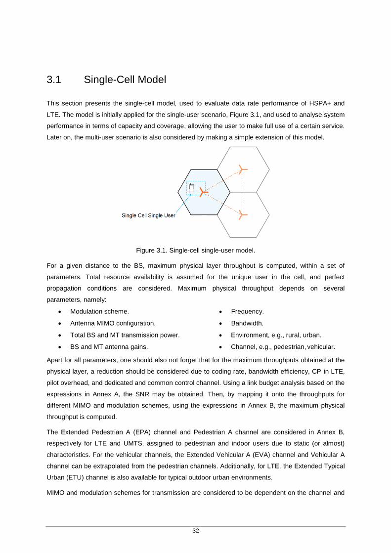
32
3.1 Single-Cell Model
This section presents the single-cell model, used to evaluate data rate performance of HSPA+ and
LTE. The model is initially applied for the single-user scenario, Figure 3.1, and used to analyse system
performance in terms of capacity and coverage, allowing the user to make full use of a certain service.
Later on, the multi-user scenario is also considered by making a simple extension of this model.
Figure 3.1. Single-cell single-user model.
For a given distance to the BS, maximum physical layer throughput is computed, within a set of
parameters. Total resource availability is assumed for the unique user in the cell, and perfect
propagation conditions are considered. Maximum physical throughput depends on several
parameters, namely:
Modulation scheme.
Antenna MIMO configuration.
Total BS and MT transmission power.
BS and MT antenna gains.
Frequency.
Bandwidth.
Environment, e.g., rural, urban.
Channel, e.g., pedestrian, vehicular.
Apart for all parameters, one should also not forget that for the maximum throughputs obtained at the
physical layer, a reduction should be considered due to coding rate, bandwidth efficiency, CP in LTE,
pilot overhead, and dedicated and common control channel. Using a link budget analysis based on the
expressions in Annex A, the SNR may be obtained. Then, by mapping it onto the throughputs for
different MIMO and modulation schemes, using the expressions in Annex B, the maximum physical
throughput is computed.
The Extended Pedestrian A (EPA) channel and Pedestrian A channel are considered in Annex B,
respectively for LTE and UMTS, assigned to pedestrian and indoor users due to static (or almost)
characteristics. For the vehicular channels, the Extended Vehicular A (EVA) channel and Vehicular A
channel can be extrapolated from the pedestrian channels. Additionally, for LTE, the Extended Typical
Urban (ETU) channel is also available for typical outdoor urban environments.
MIMO and modulation schemes for transmission are considered to be dependent on the channel and
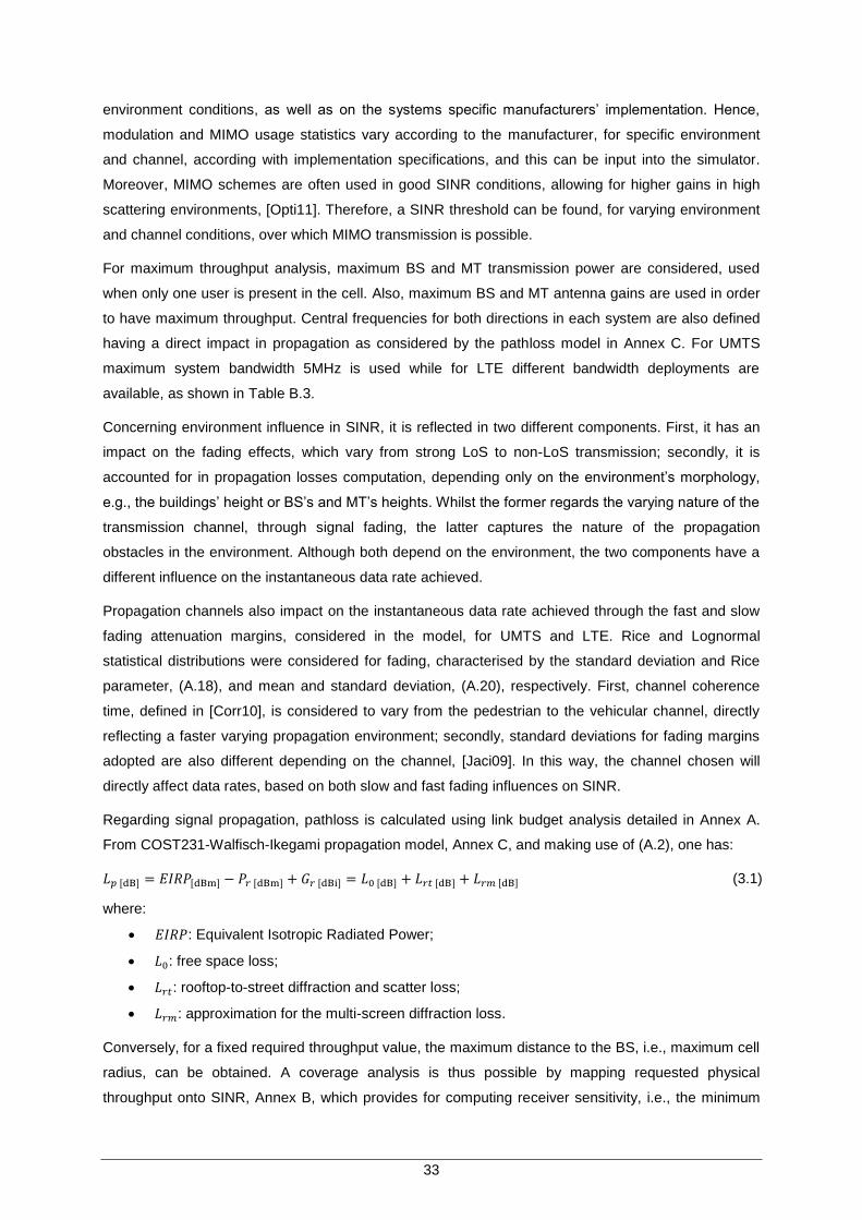
33
environment conditions, as well as on the systems specific manufacturers‟ implementation. Hence,
modulation and MIMO usage statistics vary according to the manufacturer, for specific environment
and channel, according with implementation specifications, and this can be input into the simulator.
Moreover, MIMO schemes are often used in good SINR conditions, allowing for higher gains in high
scattering environments, [Opti11]. Therefore, a SINR threshold can be found, for varying environment
and channel conditions, over which MIMO transmission is possible.
For maximum throughput analysis, maximum BS and MT transmission power are considered, used
when only one user is present in the cell. Also, maximum BS and MT antenna gains are used in order
to have maximum throughput. Central frequencies for both directions in each system are also defined
having a direct impact in propagation as considered by the pathloss model in Annex C. For UMTS
maximum system bandwidth 5MHz is used while for LTE different bandwidth deployments are
available, as shown in Table B.3.
Concerning environment influence in SINR, it is reflected in two different components. First, it has an
impact on the fading effects, which vary from strong LoS to non-LoS transmission; secondly, it is
accounted for in propagation losses computation, depending only on the environment‟s morphology,
e.g., the buildings‟ height or BS‟s and MT‟s heights. Whilst the former regards the varying nature of the
transmission channel, through signal fading, the latter captures the nature of the propagation
obstacles in the environment. Although both depend on the environment, the two components have a
different influence on the instantaneous data rate achieved.
Propagation channels also impact on the instantaneous data rate achieved through the fast and slow
fading attenuation margins, considered in the model, for UMTS and LTE. Rice and Lognormal
statistical distributions were considered for fading, characterised by the standard deviation and Rice
parameter, (A.18), and mean and standard deviation, (A.20), respectively. First, channel coherence
time, defined in [Corr10], is considered to vary from the pedestrian to the vehicular channel, directly
reflecting a faster varying propagation environment; secondly, standard deviations for fading margins
adopted are also different depending on the channel, [Jaci09]. In this way, the channel chosen will
directly affect data rates, based on both slow and fast fading influences on SINR.
Regarding signal propagation, pathloss is calculated using link budget analysis detailed in Annex A.
From COST231-Walfisch-Ikegami propagation model, Annex C, and making use of (A.2), one has:
(3.1) (3.
1) where:
: Equivalent Isotropic Radiated Power;
: free space loss;
: rooftop-to-street diffraction and scatter loss;
: approximation for the multi-screen diffraction loss.
Conversely, for a fixed required throughput value, the maximum distance to the BS, i.e., maximum cell
radius, can be obtained. A coverage analysis is thus possible by mapping requested physical
throughput onto SINR, Annex B, which provides for computing receiver sensitivity, i.e., the minimum
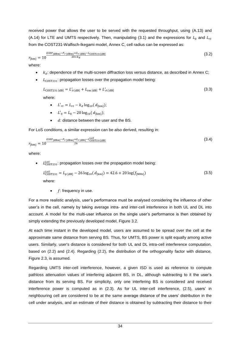
34
received power that allows the user to be served with the requested throughput, using (A.13) and
(A.14) for LTE and UMTS respectively. Then, manipulating (3.1) and the expressions for and
from the COST231-Walfisch-Ikegami model, Annex C, cell radius can be expressed as:
(3.2) (
3.
2)
where:
: dependence of the multi-screen diffraction loss versus distance, as described in Annex C;
: propagation losses over the propagation model being:
(3.3) (3.
3) where:
;
;
: distance between the user and the BS.
For LoS conditions, a similar expression can be also derived, resulting in:
(3.4) (
3.
4)
where:
: propagation losses over the propagation model being:
(3.5) (
3.
3) where:
: frequency in use.
For a more realistic analysis, user‟s performance must be analysed considering the influence of other
user‟s in the cell, namely by taking average intra- and inter-cell interference in both UL and DL into
account. A model for the multi-user influence on the single user‟s performance is then obtained by
simply extending the previously developed model, Figure 3.2.
At each time instant in the developed model, users are assumed to be spread over the cell at the
approximate same distance from serving BS. Thus, for UMTS, BS power is split equally among active
users. Similarly, user's distance is considered for both UL and DL intra-cell interference computation,
based on (2.2) and (2.4). Regarding (2.2), the distribution of the orthogonality factor with distance,
Figure 2.3, is assumed.
Regarding UMTS inter-cell interference, however, a given ISD is used as reference to compute
pathloss attenuation values of interfering adjacent BS, in DL, although subtracting to it the user‟s
distance from its serving BS. For simplicity, only one interfering BS is considered and received
interference power is computed as in (2.3). As for UL inter-cell interference, (2.5), users‟ in
neighbouring cell are considered to be at the same average distance of the users‟ distribution in the
cell under analysis, and an estimate of their distance is obtained by subtracting their distance to their
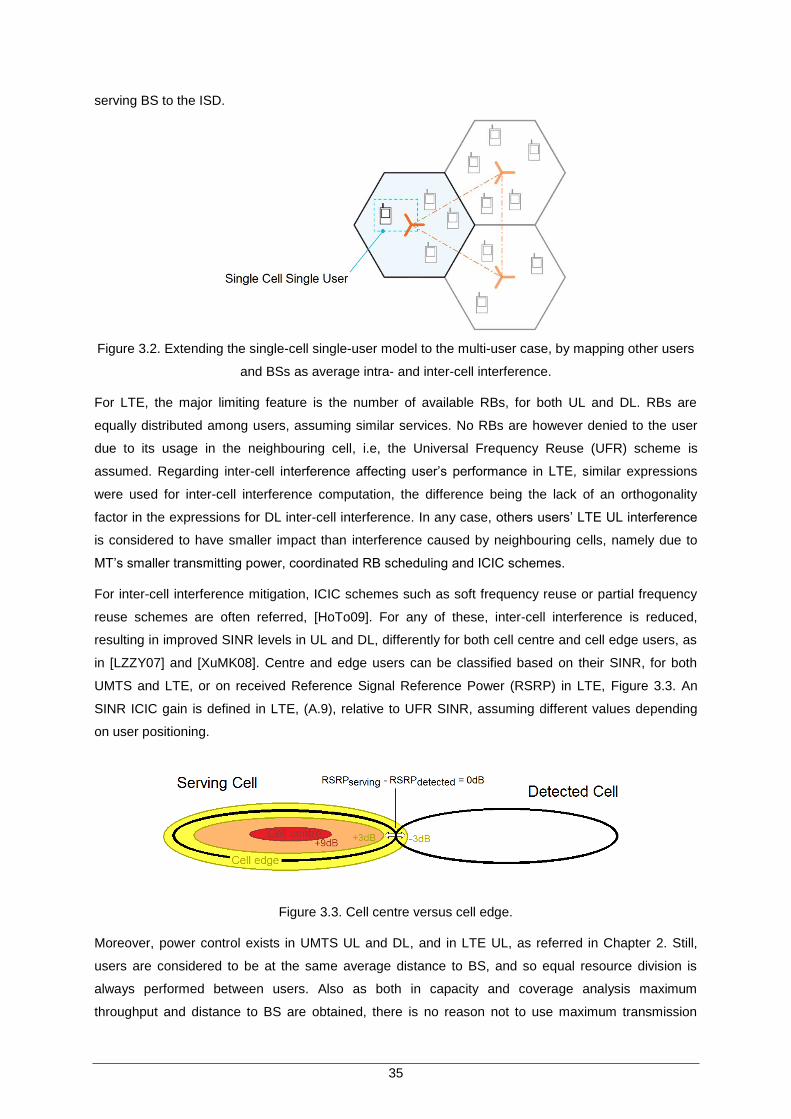
35
serving BS to the ISD.
Figure 3.2. Extending the single-cell single-user model to the multi-user case, by mapping other users
and BSs as average intra- and inter-cell interference.
For LTE, the major limiting feature is the number of available RBs, for both UL and DL. RBs are
equally distributed among users, assuming similar services. No RBs are however denied to the user
due to its usage in the neighbouring cell, i.e, the Universal Frequency Reuse (UFR) scheme is
assumed. Regarding inter-cell interference affecting user‟s performance in LTE, similar expressions
were used for inter-cell interference computation, the difference being the lack of an orthogonality
factor in the expressions for DL inter-cell interference. In any case, others users‟ LTE UL interference
is considered to have smaller impact than interference caused by neighbouring cells, namely due to
MT‟s smaller transmitting power, coordinated RB scheduling and ICIC schemes.
For inter-cell interference mitigation, ICIC schemes such as soft frequency reuse or partial frequency
reuse schemes are often referred, [HoTo09]. For any of these, inter-cell interference is reduced,
resulting in improved SINR levels in UL and DL, differently for both cell centre and cell edge users, as
in [LZZY07] and [XuMK08]. Centre and edge users can be classified based on their SINR, for both
UMTS and LTE, or on received Reference Signal Reference Power (RSRP) in LTE, Figure 3.3. An
SINR ICIC gain is defined in LTE, (A.9), relative to UFR SINR, assuming different values depending
on user positioning.
Figure 3.3. Cell centre versus cell edge.
Moreover, power control exists in UMTS UL and DL, and in LTE UL, as referred in Chapter 2. Still,
users are considered to be at the same average distance to BS, and so equal resource division is
always performed between users. Also as both in capacity and coverage analysis maximum
throughput and distance to BS are obtained, there is no reason not to use maximum transmission
36
power, providing for a straightforward comparison between systems, as long as these assumptions
are clearly understood.
Also, both in UMTS and LTE, interference power is considered to be equally spread over the
transmission bandwidth, for a realistic analysis under an equally loaded system, reducing SNR for
both LTE and UMTS comparing to the single-user‟s case. Apart from the last considerations, all
additional interference due to external factors is considered to be negligible.
3.2 UMTS and LTE Simulator
Specific implementation aspects regarding the developed HSPA+ and LTE simulator are presented in
this section. First, the simulator file structure is presented, followed by the description of simulator‟s
implementation features, and finally a global simulator evaluation is performed.
3.2.1 Simulator Overview
The simulator was developed in C++ and is composed by two main components, each one dedicated
to one of the two systems, UMTS and LTE, and able to perform both capacity and coverage analyses.
Inside each of these, a link budget analysis module exists for both UL and DL. Parallel to the
simulators, two separate modules exist, the pathloss propagation model and the channel simulation,
used to simulate propagation conditions, Figure 3.4.
Figure 3.4. UMTS and LTE Simulator‟s architecture.
The simulator receives the input parameters either directly typed in the interface developed or also by
loading Excel input files, in Comma-Separated Values (CSV) format. Output results are always
presented in a CSV Excel file, allowing to take advantage of Excel‟s capabilities for data analysis.
37
The structure chosen allows for a simpler and isolated implementation of the different modules,
particularly for different propagation models or channel simulators. More importantly, however, is that
the chosen structure allows for a comparison between systems‟ performance, by using the same
channel simulation, i.e., the same channel conditions generated, repeatedly by any of the two
simulators.
Both UMTS and LTE simulation modules receive BS‟s and UE‟s features as input for the link budgets‟
analysis, the system‟s specific parameters, namely frequencies and bandwidth, and also general
simulation parameters, namely UE‟s positions vector and simulation period. The results computation is
performed inside each link module, receiving as inputs the channel simulation and the pathloss
results, respectively from the channel simulation and the propagation model modules. Further analysis
regarding the developed simulator is presented in the simulator‟s user manual, Annex E.
3.2.2 UMTS and LTE Implementation Analysis
The modules have the purpose to do the main overall calculations obtaining the coverage and
capacity analyses for both systems, through an instantaneous snapshot approach, i.e., for a set of
defined time frames. To perform the single cell analysis, some parameters are considered, which can
be modified in the simulator:
BS‟s transmission power.
MT‟s transmission power.
BS and MT antenna gain.
Noise figure.
User and cable losses.
Signalling & Control power percentage.
Central frequency.
Bandwidth.
Modulation usage.
MIMO usage threshold.
Slow and fast fading margins.
Environment.
Channel.
Neighbouring BS‟s transmission power.
Neighbouring MT‟s transmission power.
Radio parameters, such as DL and UL transmission power, MT antenna gain, user and cable losses
and noise figure are considered the same for UMTS and LTE, being used in the simulation modules.
Specifically for DL and UL transmission powers, the same power was considered for both systems in
order to perform a fair comparison. Thus, although MT categories are a relevant constraint to
maximum user throughput, this will not be taken into account, assuming that a MT supports all
available throughputs.
Additionally, it should be considered that part of the transmission power is used for signalling and
control purposes. Namely for UMTS, the BS power split between signalling and control and user data
varies with the operating Release, as referred in Section 2.1.3. For LTE DL, one OFDM symbol is
discounted per RB and in UL, one SC-FDMA symbol, due to the reference signals, [Jaci09].
Regarding LTE DL signalling, the symbols occupied by the P-SCH and S-SCH are neglected here,
since they only account for 12 OFDM symbols in a frame, corresponding to percentages as low as
0.2% in the best case [Duar08].
38
Frequency and bandwidth, LTE specific variables, together with modulation and antenna configuration
are performance key parameters, heavily affecting achievable maximum user data rate. Considering
an analysis on the systems‟ capacity, maximum number of available codes is considered for UMTS
(15 codes in DL) whereas for LTE variable bandwidth can be chosen in the simulator, as in Table B.3.
The comparison between UMTS and LTE for the same bandwidth (5 MHz) or for maximum system
capacity (20 MHz in LTE) is thus possible.
Regarding antenna configurations, different schemes were considered: SISO, SIMO and MIMO.
Additionally, for LTE DL also a MISO configuration was taken into account. Maximum physical layer
throughput values are given as a function of the measured SNR by the expressions in Annex B,
obtained based on the 3GPP documentation and on MIMO models explained in Annex D. For the
MIMO configurations of both systems, transmission modes providing for maximum throughputs were
considered, i.e., considering spatial multiplexing transmission schemes and not transmit or receive
diversity schemes. However, an SINR level was defined as threshold for the usage of MIMO, in
particular, for each environment, due to the correlation of MIMO transmissions with the good SINR
conditions and with the scattering characteristics of the environment, as referred in Section 3.1.
Regarding modulation, while usage statistics can be specified for different schemes, throughput
calculation can also be done for each modulation scheme available and the best scheme, i.e., the one
that maximises throughput is chosen, simulating AMC techniques in both LTE and UMTS. While the
former is adopted for comparison with measured data, the latter is employed for all other capacity and
coverage analysis. Due to lack of information and to the complexity involved, adaptive coding rate is
not exploited, and only one coding scheme is considered for each modulation scheme and antenna
configuration as shown in Annex B.
Slow and fast fading margins, computed in the channel simulation module, are both probabilistic
distributions, given by Rice, (A.18), and Lognormal distributions, (A.20). Distributions‟ standard
deviations, K parameter for the Rice distribution, and channel coherence times are all input into the
simulator. Fading margins are computed in the channel module, at each coherence time interval, for
both UL and DL.
Particularly for Rice fading, different values for the K parameter were chosen according to the
environment. From the three environments implemented, Axial, Urban and Dense Urban, the Axial
benefits from LoS transmission reflected by a higher value for K, comparing to the Urban and Dense
Urban environments. Apart from this, different building configurations are taken for the Urban and
Dense Urban environments, having an influence in obtained pathloss values for these environments.
For the pedestrian and vehicular channels, due to the information available, different implementations
were considered inside each system simulator. Regarding UMTS, the pedestrian channel is based on
the data for the Pedestrian A channel, as shown in Annex B, and the vehicular channel is also
obtained based on this results as detailed in Annex B. For LTE, the pedestrian channel is obtained
based on the data for the EPA5Hz channel, and for the vehicular channel the ETU70Hz‟s results are
used for the Urban and Dense Urban environments while the extrapolation based on EPA5Hz‟s
results, similar to UMTS‟s, is taken for the Axial environment, Annex B.
39
Interference power is computed differently in each system module, as intra-cell interference exists in
UMTS. Regarding inter-cell interference in both systems, it is computed as detailed in Section 3.1, i.e.,
considering the user distance to the interfering BS, in DL, and the average neighbouring cell users‟
distance to the serving BS, in UL. Neighbouring BS‟s and MT‟s power are also inputted into the
simulator, making it possible to consider a neighbouring BS transmitting at 50% of maximum power,
for example, reflecting a lower cell load situation. Intra-cell interference only exists in UMTS, and as
average users‟ distance to BS is known, received interference power in UL and DL is simply
computed.
For both user and interference power received, the propagation model module computes pathloss, as
in Annex C, depending on environment characterisation and distance between emitting and receiving
antennas. Conversely, for coverage analysis, the module computes the and , used in
(3.2) and (3.4).
Furthermore, for simulation, three main parameters are defined as inputs, depending on the type of
analysis required. For the capacity analysis, distance to BS statistics, i.e., mean and standard
deviation of a Gaussian distribution, and number of cell users are required for single- and multi-user
analysis. Differently, for service coverage analysis, service required data rate and number of cell users
are inputted, so to obtain maximum cell range, for which the user is still served. Apart from these, also
the simulation period is defined for simulation, independently of the performed analysis.
Output results vary depending on the analysis, either capacity or coverage. Instantaneous user‟s
distance to BS, pathloss, fading margins, SINR, throughput, modulation and antenna configuration are
output for the first, while pathloss, fading margins, cell range, modulation and antenna configuration
for the second, for UL and DL by both UMTS and LTE simulators.
3.3 Simulator Assessment and Model Evaluation
Prior to results analysis, the simulator was assessed, namely regarding the validity of the output and
the necessary number of simulations that ensure statistical relevance of the results. For this purpose,
statistical parameters such as the average, standard deviation and correlation coefficients of the
results were analysed. The simulator, i.e., the implemented model, is further compared with the
measured results obtained in subsequent chapters.
Output results mean, standard deviation and correlation coefficient between data sets were obtained
using (3.6), (3.7) and (3.8), as defined in [Mora10].
(3.6) (
3.
6)
where:
: sample ;
: number of samples.
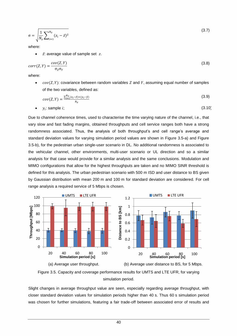
40
(3.7) (
3.
7)
where:
: average value of sample set .
(3.8) (
3.
8)
where:
: covariance between random variables and , assuming equal number of samples
of the two variables, defined as:
(3.9) (
3.
7)
: sample ; (3.10)
Due to channel coherence times, used to characterise the time varying nature of the channel, i.e., that
vary slow and fast fading margins, obtained throughputs and cell service ranges both have a strong
randomness associated. Thus, the analysis of both throughput‟s and cell range‟s average and
standard deviation values for varying simulation period values are shown in Figure 3.5-a) and Figure
3.5-b), for the pedestrian urban single-user scenario in DL. No additional randomness is associated to
the vehicular channel, other environments, multi-user scenario or UL direction and so a similar
analysis for that case would provide for a similar analysis and the same conclusions. Modulation and
MIMO configurations that allow for the highest throughputs are taken and no MIMO SINR threshold is
defined for this analysis. The urban pedestrian scenario with 500 m ISD and user distance to BS given
by Gaussian distribution with mean 200 m and 100 m for standard deviation are considered. For cell
range analysis a required service of 5 Mbps is chosen.
(a) Average user throughput. (b) Average user distance to BS, for 5 Mbps.
Figure 3.5. Capacity and coverage performance results for UMTS and LTE UFR, for varying
simulation period.
Slight changes in average throughput value are seen, especially regarding average throughput, with
closer standard deviation values for simulation periods higher than 40 s. Thus 60 s simulation period
was chosen for further simulations, featuring a fair trade-off between associated error of results and
0
20
40
60
80
100
120
20 40 60 80 100
Th
rou
gh
pu
t [M
bp
s]
Simulation period [s]
UMTS LTE UFR
0
0.2
0.4
0.6
0.8
1
1.2
20 40 60 80 100
Dis
tan
ce
to
BS
[k
m]
Simulation period [s]
UMTS LTE UFR
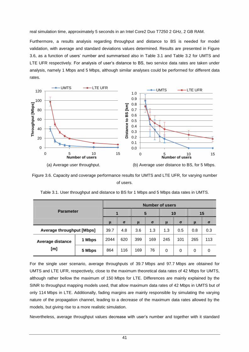
41
real simulation time, approximately 5 seconds in an Intel Core2 Duo T7250 2 GHz, 2 GB RAM.
Furthermore, a results analysis regarding throughput and distance to BS is needed for model
validation, with average and standard deviations values determined. Results are presented in Figure
3.6, as a function of users‟ number and summarised also in Table 3.1 and Table 3.2 for UMTS and
LTE UFR respectively. For analysis of user‟s distance to BS, two service data rates are taken under
analysis, namely 1 Mbps and 5 Mbps, although similar analyses could be performed for different data
rates.
(a) Average user throughput. (b) Average user distance to BS, for 5 Mbps.
Figure 3.6. Capacity and coverage performance results for UMTS and LTE UFR, for varying number
of users.
Table 3.1. User throughput and distance to BS for 1 Mbps and 5 Mbps data rates in UMTS.
Parameter
Number of users
1 5 10 15
Average throughput [Mbps] 39.7 4.8 3.6 1.3 1.3 0.5 0.8 0.3
Average distance
[m]
1 Mbps 2044 620 399 169 245 101 265 113
5 Mbps 864 116 169 76 0 0 0 0
For the single user scenario, average throughputs of 39.7 Mbps and 97.7 Mbps are obtained for
UMTS and LTE UFR, respectively, close to the maximum theoretical data rates of 42 Mbps for UMTS,
although rather bellow the maximum of 150 Mbps for LTE. Differences are mainly explained by the
SINR to throughput mapping models used, that allow maximum data rates of 42 Mbps in UMTS but of
only 114 Mbps in LTE. Additionally, fading margins are mainly responsible by simulating the varying
nature of the propagation channel, leading to a decrease of the maximum data rates allowed by the
models, but giving rise to a more realistic simulation.
Nevertheless, average throughput values decrease with user‟s number and together with it standard
0
20
40
60
80
100
120
0 5 10 15
Th
rou
gh
pu
t [M
bp
s]
Number of users
UMTS LTE UFR
0.0
0.1
0.2
0.3
0.4
0.5
0.6
0.7
0.8
0.9
1.0
0 5 10 15
Dis
tan
ce
to
BS
[k
m]
Number of users
UMTS LTE UFR

42
deviation, naturally, due to the smaller absolute throughput values. A great drop in average throughput
is seen from the single- to the multi-user scenario, as expected, in both UMTS and LTE UFR.
Whereas for UMTS throughput is mainly reduced by the presence of intra-cell interference, rising with
the number of cell users, in LTE the split of available RBs between users also reduces data rates, as it
is clearly seen in results in Table 3.2. Smaller growths in intra-cell interference and decreases in RBs
per user occur, however, for higher user‟s number in the multi-user scenario, resulting in smaller
decrease in average throughput.
Table 3.2. User throughput and distance to BS for 1 Mbps and 5 Mbps data rates in LTE UFR.
Parameter
Number of users
1 5 10 15
Average throughput [Mbps] 97.7 9.5 19.6 1.3 9.8 0.5 6.5 0.3
Average distance
[m]
1 Mbps 880 236 682 221 531 171 465 176
5 Mbps 768 116 346 126 243 81 167 48
Regarding cell range, for any of the considered services, it decreases with users‟ number but also with
the absolute value of the required service throughput. For higher user‟s number, users‟ may even not
be served, as it is seen with UMTS for more than 10 users, due to the limited BS transmission power
and limiting intra- and inter-cell interference power levels. Regarding LTE the limitation is still in the
number of RB‟s per user. Nevertheless, UMTS still provides for higher cell ranges for the single-user
scenario in 1 Mbps and in 5 Mbps assured data rates.
43
Chapter 4
Results Analysis
4 Models
This chapter presents the results from the LTE measurements campaign performed as well as the
simulator results for both UMTS and LTE. Measurements results are initially analysed, describing the
scenario used and drawing different analysis regarding SNIR and physical throughput. A comparison
between measurements‟ and simulations‟ results is then performed, comparing SINR and throughput
for varying channel and environment. Finally, UMTS‟s and LTE‟s simulation results are compared, and
performance gains computed, presenting conclusions on systems‟ capacity and coverage.
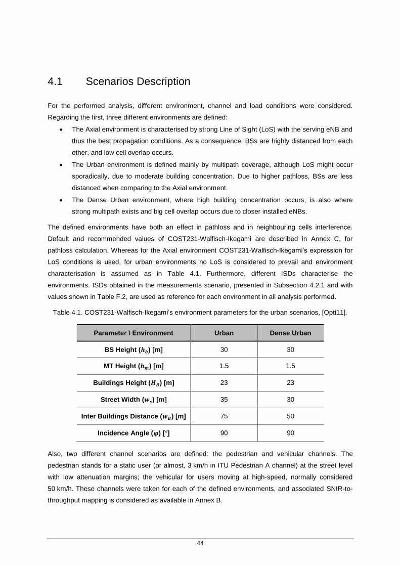
44
4.1 Scenarios Description
For the performed analysis, different environment, channel and load conditions were considered.
Regarding the first, three different environments are defined:
The Axial environment is characterised by strong Line of Sight (LoS) with the serving eNB and
thus the best propagation conditions. As a consequence, BSs are highly distanced from each
other, and low cell overlap occurs.
The Urban environment is defined mainly by multipath coverage, although LoS might occur
sporadically, due to moderate building concentration. Due to higher pathloss, BSs are less
distanced when comparing to the Axial environment.
The Dense Urban environment, where high building concentration occurs, is also where
strong multipath exists and big cell overlap occurs due to closer installed eNBs.
The defined environments have both an effect in pathloss and in neighbouring cells interference.
Default and recommended values of COST231-Walfisch-Ikegami are described in Annex C, for
pathloss calculation. Whereas for the Axial environment COST231-Walfisch-Ikegami‟s expression for
LoS conditions is used, for urban environments no LoS is considered to prevail and environment
characterisation is assumed as in Table 4.1. Furthermore, different ISDs characterise the
environments. ISDs obtained in the measurements scenario, presented in Subsection 4.2.1 and with
values shown in Table F.2, are used as reference for each environment in all analysis performed.
Table 4.1. COST231-Walfisch-Ikegami‟s environment parameters for the urban scenarios, [Opti11].
Parameter \ Environment Urban Dense Urban
BS Height ( ) [m] 30 30
MT Height ( ) [m] 1.5 1.5
Buildings Height ( ) [m] 23 23
Street Width ( ) [m] 35 30
Inter Buildings Distance ( ) [m] 75 50
Incidence Angle ( ) [ ] 90 90
Also, two different channel scenarios are defined: the pedestrian and vehicular channels. The
pedestrian stands for a static user (or almost, 3 km/h in ITU Pedestrian A channel) at the street level
with low attenuation margins; the vehicular for users moving at high-speed, normally considered
50 km/h. These channels were taken for each of the defined environments, and associated SNIR-to-
throughput mapping is considered as available in Annex B.
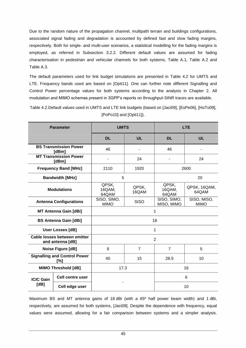
45
Due to the random nature of the propagation channel, multipath terrain and buildings configurations,
associated signal fading and degradation is accounted by defined fast and slow fading margins,
respectively. Both for single- and multi-user scenarios, a statistical modelling for the fading margins is
employed, as referred in Subsection 3.2.2. Different default values are assumed for fading
characterisation in pedestrian and vehicular channels for both systems, Table A.1, Table A.2 and
Table A.3.
The default parameters used for link budget simulations are presented in Table 4.2 for UMTS and
LTE. Frequency bands used are based on [Opti11]. One can further note different Signalling and
Control Power percentage values for both systems according to the analysis in Chapter 2. All
modulation and MIMO schemes present in 3GPP‟s reports on throughput-SINR traces are available.
Table 4.2.Default values used in UMTS and LTE link budgets (based on [Jaci09], [EsPe06], [HoTo09],
[PoPo10] and [Opti11]).
Parameter UMTS LTE
DL UL DL UL
BS Transmission Power [dBm]
46 - 46 -
MT Transmission Power [dBm]
- 24 - 24
Frequency Band [MHz] 2110 1920 2600
Bandwidth [MHz] 5
20
Modulations QPSK,
16QAM, 64QAM
QPSK, 16QAM
QPSK, 16QAM, 64QAM
QPSK, 16QAM, 64QAM
Antenna Configurations SISO, SIMO,
MIMO SISO
SISO, SIMO, MISO, MIMO
SISO, MISO, MIMO
MT Antenna Gain [dBi] 1
BS Antenna Gain [dBi] 18
User Losses [dB] 1
Cable losses between emitter and antenna [dB]
2
Noise Figure [dB] 9 7 7 5
Signalling and Control Power [%]
40 15 28.5 10
MIMO Threshold [dB] 17.3 16
ICIC Gain [dB]
Cell centre user -
6
Cell edge user 10
Maximum BS and MT antenna gains of 18 dBi (with a 65º half power beam width) and 1 dBi,
respectively, are assumed for both systems, [Jaci09]. Despite the dependence with frequency, equal
values were assumed, allowing for a fair comparison between systems and a simpler analysis.
46
Additionally, both equipment gains are manufacturer dependent and may vary according to the type of
hardware.
Identical transmission power values were also set in order for a fair system‟s comparison. Actually,
some HSPA+ sites exist that are already being supplied by 40 W. However, general values are below
this target, according to [Jaci09], namely 43 or 44.7 dBm for macro-cells. For LTE, BSs are commonly
deployed with 46 dBm maximum transmission power, [Opti11].
As the human body absorbs energy, a body loss margin of 1 dB is established. Moreover, losses
generated by feeders, connectors and all external equipment between the antenna and the BS
receiver are considered. Although varying with the equipment type and manufacturers and operators
implementation issues, a margin of 2 dB is used.
A 5 MHz bandwidth is assumed for UMTS transmission whereas for LTE the maximum of 20 MHz is
used. Although the same bandwidth could be considered, for LTE the system is designed to allow for
higher bandwidths, differently than for UMTS, and thus one should not restrict itself to a comparison
using 5 MHz LTE. Nevertheless, if the latter scenario is the case, the same results are applicable
although dividing maximum throughputs obtained by a factor of 4, assuming equal spectral efficiency
for 5 and 20 MHz, Table B.3.
A SINR threshold level is defined for both systems, above which MIMO transmission can be
scheduled. For UMTS, the reference threshold value was adapted from [Bati08], where it was
considered as SINR threshold for the maximum throughputs in DL for HSPA+. For LTE, the assumed
value is obtained in Section 4.2, based on measurements results.
Additionally for LTE ICIC variant, a higher SINR gain is considered for cell edge users than for cell
centre users, based on results in [LZZY07] and [XuMK08]. Although different gain values could be
assumed, depending on the environment, due to different interference levels felt in each environment,
for simplicity no differences are here assumed. Moreover, the obtained gain in SINR is largely
dependent on the ICIC scheme chosen, e.g. soft frequency reuse or partial frequency reuse schemes,
and in practical implementation considerations. Again, a simple but meaningful solution is preferred.
Interference power is computed as defined by the Single-Cell model developed, both intra- and inter-
cell. However, although users in the cell under study are considered to be at maximum load, i.e.,
transmitting with maximum power in both UL and DL, neighbouring cells are considered to serve the
same amount of users but at 50% of maximum transmitted power, [Opti11]. Therefore, in DL,
neighbouring BS‟s maximum transmitted power is 42.97 dBm, Table 4.3, and in UL, neighbouring
MTs‟ maximum transmitted power is 21 dBm, 50% of the respective MT power in Table 4.2.
Regarding the coverage analysis, i.e., distance to BS as a function of number of users‟ analysis,
different services were considered to provide a broader coverage of vast types of services possible.
Particularly, three service types were considered: a Web service, for UL and DL, requiring typical data
rates of 1 Mbps according to [Jaci09]; a video streaming service, for DL, with typical maximum
throughput values of 5 Mbps for MPEG-2‟s primary distribution according to [Pere11]; and a File
Transfer Protocol (FTP) service, considering a possible requested throughput of 10 Mbps, Table 4.4.
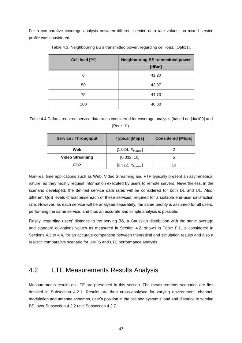
47
For a comparative coverage analysis between different service data rate values, no mixed service
profile was considered.
Table 4.3. Neighbouring BS‟s transmitted power, regarding cell load, [Opti11].
Cell load [%] Neighbouring BS transmitted power
[dBm]
0 41.20
50 42.97
75 44.73
100 46.00
Table 4.4.Default required service data rates considered for coverage analysis (based on [Jaci09] and
[Pere11]).
Service / Throughput Typical [Mbps] Considered [Mbps]
Web [1.024, ] 2
Video Streaming [0.032, 10] 5
FTP [0.512, ] 10
Non-real time applications such as Web, Video Streaming and FTP typically present an asymmetrical
nature, as they mostly request information executed by users to remote servers. Nevertheless, in the
scenario developed, the defined service data rates will be considered for both DL and UL. Also,
different QoS levels characterise each of these services, required for a suitable end-user satisfaction
rate. However, as each service will be analysed separately, the same priority is assumed for all users,
performing the same service, and thus an accurate and simple analysis is possible.
Finally, regarding users‟ distance to the serving BS, a Gaussian distribution with the same average
and standard deviations values as measured in Section 4.2, shown in Table F.1, is considered in
Sections 4.3 to 4.4, for an accurate comparison between theoretical and simulation results and also a
realistic comparative scenario for UMTS and LTE performance analysis.
4.2 LTE Measurements Results Analysis
Measurements results on LTE are presented in this section. The measurements scenarios are first
detailed in Subsection 4.2.1. Results are then cross-analysed for varying environment, channel,
modulation and antenna schemes, user‟s position in the cell and system‟s load and distance to serving
BS, over Subsection 4.2.2 until Subsection 4.2.7.
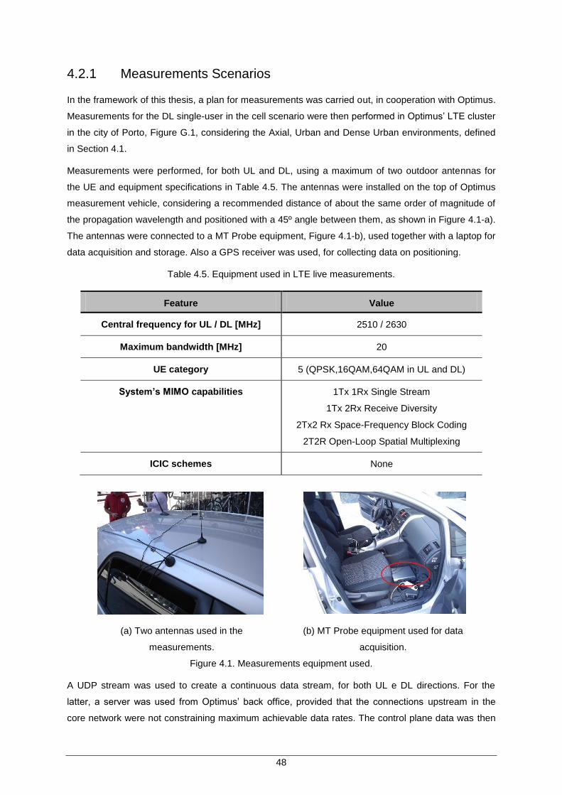
48
4.2.1 Measurements Scenarios
In the framework of this thesis, a plan for measurements was carried out, in cooperation with Optimus.
Measurements for the DL single-user in the cell scenario were then performed in Optimus‟ LTE cluster
in the city of Porto, Figure G.1, considering the Axial, Urban and Dense Urban environments, defined
in Section 4.1.
Measurements were performed, for both UL and DL, using a maximum of two outdoor antennas for
the UE and equipment specifications in Table 4.5. The antennas were installed on the top of Optimus
measurement vehicle, considering a recommended distance of about the same order of magnitude of
the propagation wavelength and positioned with a 45º angle between them, as shown in Figure 4.1-a).
The antennas were connected to a MT Probe equipment, Figure 4.1-b), used together with a laptop for
data acquisition and storage. Also a GPS receiver was used, for collecting data on positioning.
Table 4.5. Equipment used in LTE live measurements.
Feature Value
Central frequency for UL / DL [MHz] 2510 / 2630
Maximum bandwidth [MHz] 20
UE category 5 (QPSK,16QAM,64QAM in UL and DL)
System’s MIMO capabilities 1Tx 1Rx Single Stream
1Tx 2Rx Receive Diversity
2Tx2 Rx Space-Frequency Block Coding
2T2R Open-Loop Spatial Multiplexing
ICIC schemes None
(a) Two antennas used in the
measurements.
(b) MT Probe equipment used for data
acquisition.
Figure 4.1. Measurements equipment used.
A UDP stream was used to create a continuous data stream, for both UL e DL directions. For the
latter, a server was used from Optimus‟ back office, provided that the connections upstream in the
core network were not constraining maximum achievable data rates. The control plane data was then
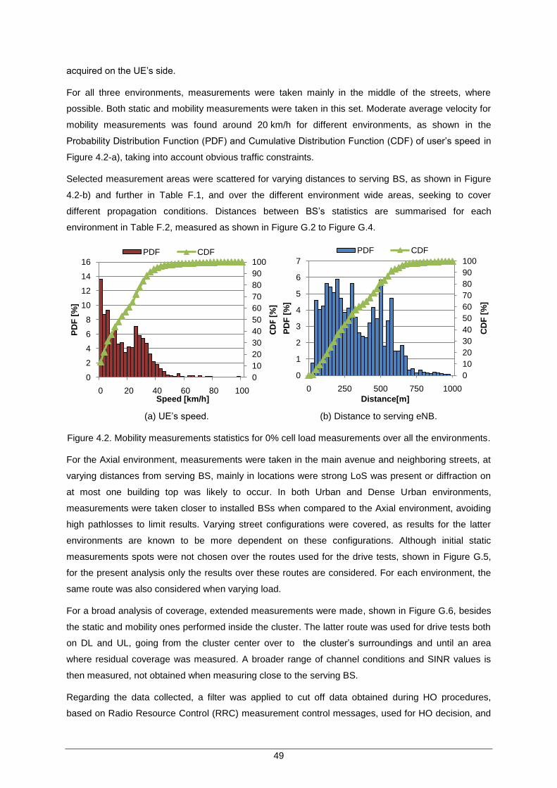
49
acquired on the UE‟s side.
For all three environments, measurements were taken mainly in the middle of the streets, where
possible. Both static and mobility measurements were taken in this set. Moderate average velocity for
mobility measurements was found around 20 km/h for different environments, as shown in the
Probability Distribution Function (PDF) and Cumulative Distribution Function (CDF) of user‟s speed in
Figure 4.2-a), taking into account obvious traffic constraints.
Selected measurement areas were scattered for varying distances to serving BS, as shown in Figure
4.2-b) and further in Table F.1, and over the different environment wide areas, seeking to cover
different propagation conditions. Distances between BS‟s statistics are summarised for each
environment in Table F.2, measured as shown in Figure G.2 to Figure G.4.
(a) UE‟s speed. (b) Distance to serving eNB.
Figure 4.2. Mobility measurements statistics for 0% cell load measurements over all the environments.
For the Axial environment, measurements were taken in the main avenue and neighboring streets, at
varying distances from serving BS, mainly in locations were strong LoS was present or diffraction on
at most one building top was likely to occur. In both Urban and Dense Urban environments,
measurements were taken closer to installed BSs when compared to the Axial environment, avoiding
high pathlosses to limit results. Varying street configurations were covered, as results for the latter
environments are known to be more dependent on these configurations. Although initial static
measurements spots were not chosen over the routes used for the drive tests, shown in Figure G.5,
for the present analysis only the results over these routes are considered. For each environment, the
same route was also considered when varying load.
For a broad analysis of coverage, extended measurements were made, shown in Figure G.6, besides
the static and mobility ones performed inside the cluster. The latter route was used for drive tests both
on DL and UL, going from the cluster center over to the cluster‟s surroundings and until an area
where residual coverage was measured. A broader range of channel conditions and SINR values is
then measured, not obtained when measuring close to the serving BS.
Regarding the data collected, a filter was applied to cut off data obtained during HO procedures,
based on Radio Resource Control (RRC) measurement control messages, used for HO decision, and
0
10
20
30
40
50
60
70
80
90
100
0
2
4
6
8
10
12
14
16
0 20 40 60 80 100
CD
F [%
]
PD
F [
%]
Speed [km/h]
PDF CDF
0
10
20
30
40
50
60
70
80
90
100
0
1
2
3
4
5
6
7
0 250 500 750 1000
CD
F [
%]
PD
F [
%]
Distance[m]
PDF CDF
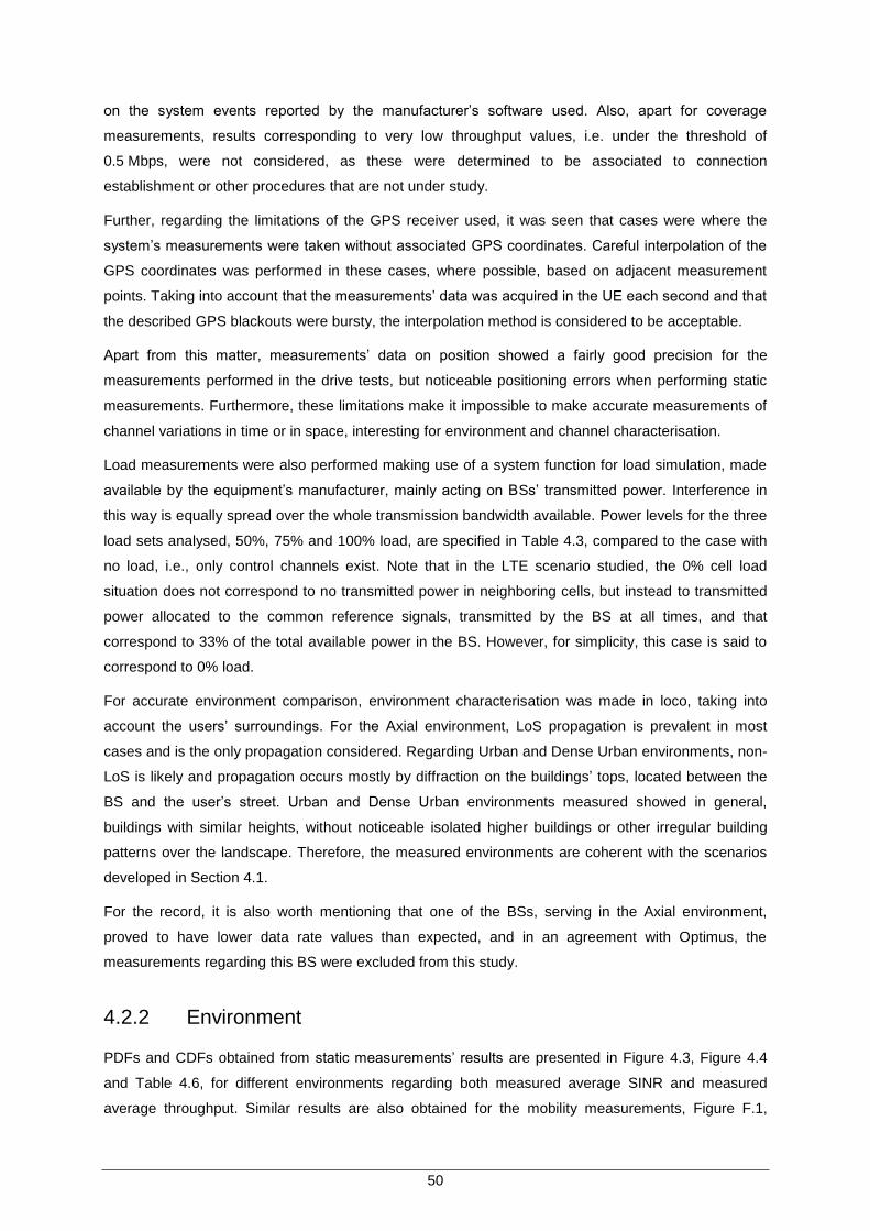
50
on the system events reported by the manufacturer‟s software used. Also, apart for coverage
measurements, results corresponding to very low throughput values, i.e. under the threshold of
0.5 Mbps, were not considered, as these were determined to be associated to connection
establishment or other procedures that are not under study.
Further, regarding the limitations of the GPS receiver used, it was seen that cases were where the
system‟s measurements were taken without associated GPS coordinates. Careful interpolation of the
GPS coordinates was performed in these cases, where possible, based on adjacent measurement
points. Taking into account that the measurements‟ data was acquired in the UE each second and that
the described GPS blackouts were bursty, the interpolation method is considered to be acceptable.
Apart from this matter, measurements‟ data on position showed a fairly good precision for the
measurements performed in the drive tests, but noticeable positioning errors when performing static
measurements. Furthermore, these limitations make it impossible to make accurate measurements of
channel variations in time or in space, interesting for environment and channel characterisation.
Load measurements were also performed making use of a system function for load simulation, made
available by the equipment‟s manufacturer, mainly acting on BSs‟ transmitted power. Interference in
this way is equally spread over the whole transmission bandwidth available. Power levels for the three
load sets analysed, 50%, 75% and 100% load, are specified in Table 4.3, compared to the case with
no load, i.e., only control channels exist. Note that in the LTE scenario studied, the 0% cell load
situation does not correspond to no transmitted power in neighboring cells, but instead to transmitted
power allocated to the common reference signals, transmitted by the BS at all times, and that
correspond to 33% of the total available power in the BS. However, for simplicity, this case is said to
correspond to 0% load.
For accurate environment comparison, environment characterisation was made in loco, taking into
account the users‟ surroundings. For the Axial environment, LoS propagation is prevalent in most
cases and is the only propagation considered. Regarding Urban and Dense Urban environments, non-
LoS is likely and propagation occurs mostly by diffraction on the buildings‟ tops, located between the
BS and the user‟s street. Urban and Dense Urban environments measured showed in general,
buildings with similar heights, without noticeable isolated higher buildings or other irregular building
patterns over the landscape. Therefore, the measured environments are coherent with the scenarios
developed in Section 4.1.
For the record, it is also worth mentioning that one of the BSs, serving in the Axial environment,
proved to have lower data rate values than expected, and in an agreement with Optimus, the
measurements regarding this BS were excluded from this study.
4.2.2 Environment
PDFs and CDFs obtained from static measurements‟ results are presented in Figure 4.3, Figure 4.4
and Table 4.6, for different environments regarding both measured average SINR and measured
average throughput. Similar results are also obtained for the mobility measurements, Figure F.1,
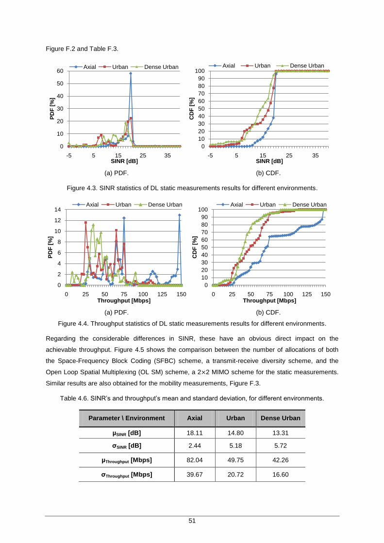
51
Figure F.2 and Table F.3.
(a) PDF. (b) CDF.
Figure 4.3. SINR statistics of DL static measurements results for different environments.
(a) PDF. (b) CDF.
Figure 4.4. Throughput statistics of DL static measurements results for different environments.
Regarding the considerable differences in SINR, these have an obvious direct impact on the
achievable throughput. Figure 4.5 shows the comparison between the number of allocations of both
the Space-Frequency Block Coding (SFBC) scheme, a transmit-receive diversity scheme, and the
Open Loop Spatial Multiplexing (OL SM) scheme, a 2 2 MIMO scheme for the static measurements.
Similar results are also obtained for the mobility measurements, Figure F.3.
Table 4.6. SINR‟s and throughput‟s mean and standard deviation, for different environments.
Parameter \ Environment Axial Urban Dense Urban
µSINR [dB] 18.11 14.80 13.31
σSINR [dB] 2.44 5.18 5.72
µThroughput [Mbps] 82.04 49.75 42.26
σThroughput [Mbps] 39.67 20.72 16.60
-5 5 15 25 35
0
10
20
30
40
50
60
SINR [dB]
PD
F [
%]
Axial Urban Dense Urban
-5 5 15 25 35
0
10
20
30
40
50
60
70
80
90
100
SINR [dB]
CD
F [
%]
Axial Urban Dense Urban
0 25 50 75 100 125 150
0
2
4
6
8
10
12
14
Throughput [Mbps]
PD
F [
%]
Axial Urban Dense Urban
0 25 50 75 100 125 150
0
10
20
30
40
50
60
70
80
90
100
Throughput [Mbps]
CD
F [
%]
Axial Urban Dense Urban
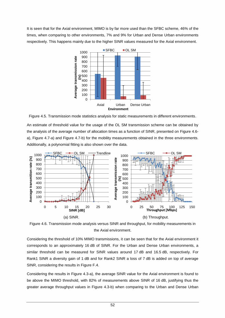
52
It is seen that for the Axial environment, MIMO is by far more used than the SFBC scheme, 46% of the
times, when comparing to other environments, 7% and 9% for Urban and Dense Urban environments
respectively. This happens mainly due to the higher SINR values measured for the Axial environment.
Figure 4.5. Transmission mode statistics analysis for static measurements in different environments.
An estimate of threshold value for the usage of the OL SM transmission scheme can be obtained by
the analysis of the average number of allocation times as a function of SINR, presented on Figure 4.6-
a), Figure 4.7-a) and Figure 4.7-b) for the mobility measurements obtained in the three environments.
Additionally, a polynomial fitting is also shown over the data.
(a) SINR. (b) Throughput.
Figure 4.6. Transmission mode analysis versus SINR and throughput, for mobility measurements in
the Axial environment.
Considering the threshold of 10% MIMO transmissions, it can be seen that for the Axial environment it
corresponds to an approximately 16 dB of SINR. For the Urban and Dense Urban environments, a
similar threshold can be measured for SINR values around 17 dB and 16.5 dB, respectively. For
Rank1 SINR a diversity gain of 1 dB and for Rank2 SINR a loss of 7 dB is added on top of average
SINR, considering the results in Figure F.4.
Considering the results in Figure 4.3-a), the average SINR value for the Axial environment is found to
be above the MIMO threshold, with 82% of measurements above SINR of 16 dB, justifying thus the
greater average throughput values in Figure 4.3-b) when comparing to the Urban and Dense Urban
0
100
200
300
400
500
600
700
800
900
1000
Axial Urban Dense Urban
Ave
rag
e t
ran
sm
iss
ion
ra
te
(/s
)
Environment
SFBC OL SM
0
100
200
300
400
500
600
700
800
900
1000
0 5 10 15 20 25 30
Ave
rag
e t
ran
sm
itio
n r
ate
(/s
)
SINR [dB]
SFBC OL SM Trendline
0
100
200
300
400
500
600
700
800
900
1000
0 25 50 75 100 125 150
Ave
rag
e t
ran
sm
iss
ion
rate
(/s
)
Throughput [Mbps]
SFBC OL SM
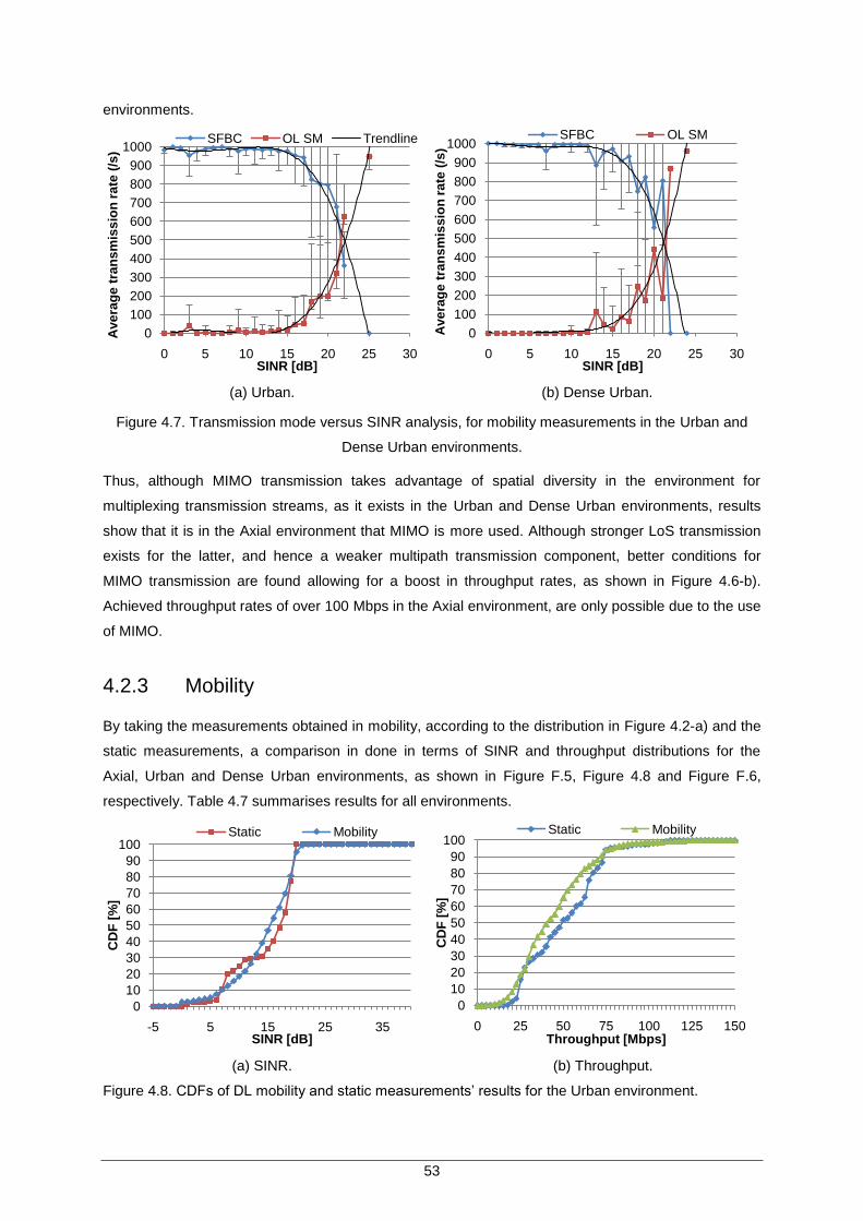
53
environments.
(a) Urban. (b) Dense Urban.
Figure 4.7. Transmission mode versus SINR analysis, for mobility measurements in the Urban and
Dense Urban environments.
Thus, although MIMO transmission takes advantage of spatial diversity in the environment for
multiplexing transmission streams, as it exists in the Urban and Dense Urban environments, results
show that it is in the Axial environment that MIMO is more used. Although stronger LoS transmission
exists for the latter, and hence a weaker multipath transmission component, better conditions for
MIMO transmission are found allowing for a boost in throughput rates, as shown in Figure 4.6-b).
Achieved throughput rates of over 100 Mbps in the Axial environment, are only possible due to the use
of MIMO.
4.2.3 Mobility
By taking the measurements obtained in mobility, according to the distribution in Figure 4.2-a) and the
static measurements, a comparison in done in terms of SINR and throughput distributions for the
Axial, Urban and Dense Urban environments, as shown in Figure F.5, Figure 4.8 and Figure F.6,
respectively. Table 4.7 summarises results for all environments.
(a) SINR. (b) Throughput.
Figure 4.8. CDFs of DL mobility and static measurements‟ results for the Urban environment.
0
100
200
300
400
500
600
700
800
900
1000
0 5 10 15 20 25 30
Ave
rag
e t
ran
sm
iss
ion
ra
te (
/s)
SINR [dB]
SFBC OL SM Trendline
0
100
200
300
400
500
600
700
800
900
1000
0 5 10 15 20 25 30
Ave
rag
e t
ran
sm
iss
ion
ra
te (
/s)
SINR [dB]
SFBC OL SM
-5 5 15 25 35
0
10
20
30
40
50
60
70
80
90
100
SINR [dB]
CD
F [
%]
Static Mobility
0 25 50 75 100 125 150
0
10
20
30
40
50
60
70
80
90
100
Throughput [Mbps]
CD
F [
%]
Static Mobility
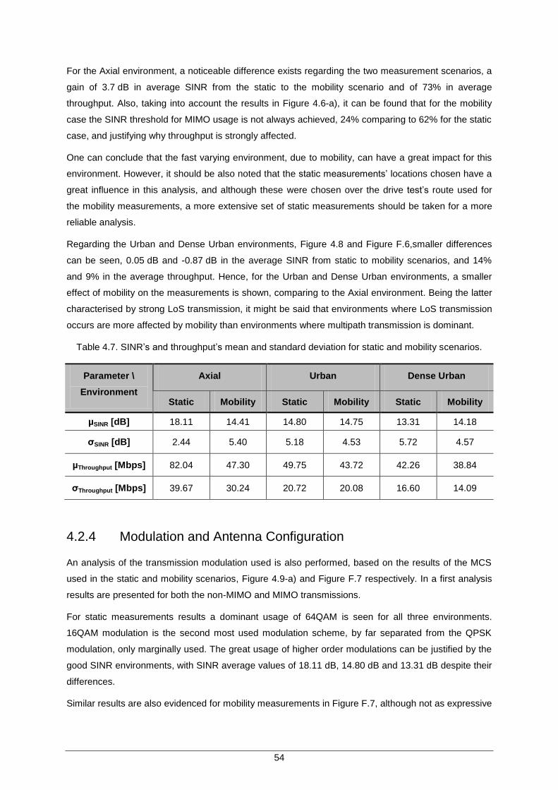
54
For the Axial environment, a noticeable difference exists regarding the two measurement scenarios, a
gain of 3.7 dB in average SINR from the static to the mobility scenario and of 73% in average
throughput. Also, taking into account the results in Figure 4.6-a), it can be found that for the mobility
case the SINR threshold for MIMO usage is not always achieved, 24% comparing to 62% for the static
case, and justifying why throughput is strongly affected.
One can conclude that the fast varying environment, due to mobility, can have a great impact for this
environment. However, it should be also noted that the static measurements‟ locations chosen have a
great influence in this analysis, and although these were chosen over the drive test‟s route used for
the mobility measurements, a more extensive set of static measurements should be taken for a more
reliable analysis.
Regarding the Urban and Dense Urban environments, Figure 4.8 and Figure F.6,smaller differences
can be seen, 0.05 dB and -0.87 dB in the average SINR from static to mobility scenarios, and 14%
and 9% in the average throughput. Hence, for the Urban and Dense Urban environments, a smaller
effect of mobility on the measurements is shown, comparing to the Axial environment. Being the latter
characterised by strong LoS transmission, it might be said that environments where LoS transmission
occurs are more affected by mobility than environments where multipath transmission is dominant.
Table 4.7. SINR‟s and throughput‟s mean and standard deviation for static and mobility scenarios.
Parameter \
Environment
Axial Urban Dense Urban
Static Mobility Static Mobility Static Mobility
µSINR [dB] 18.11 14.41 14.80 14.75 13.31 14.18
σSINR [dB] 2.44 5.40 5.18 4.53 5.72 4.57
µThroughput [Mbps] 82.04 47.30 49.75 43.72 42.26 38.84
σThroughput [Mbps] 39.67 30.24 20.72 20.08 16.60 14.09
4.2.4 Modulation and Antenna Configuration
An analysis of the transmission modulation used is also performed, based on the results of the MCS
used in the static and mobility scenarios, Figure 4.9-a) and Figure F.7 respectively. In a first analysis
results are presented for both the non-MIMO and MIMO transmissions.
For static measurements results a dominant usage of 64QAM is seen for all three environments.
16QAM modulation is the second most used modulation scheme, by far separated from the QPSK
modulation, only marginally used. The great usage of higher order modulations can be justified by the
good SINR environments, with SINR average values of 18.11 dB, 14.80 dB and 13.31 dB despite their
differences.
Similar results are also evidenced for mobility measurements in Figure F.7, although not as expressive
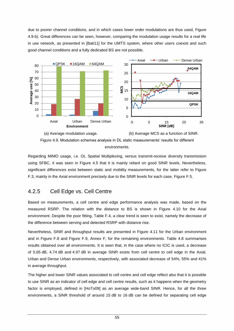
55
due to poorer channel conditions, and in which cases lower order modulations are thus used, Figure
4.9-b). Great differences can be seen, however, comparing the modulation usage results for a real life
in use network, as presented in [Bati11] for the UMTS system, where other users coexist and such
good channel conditions and a fully dedicated BS are not possible.
(a) Average modulation usage. (b) Average MCS as a function of SINR.
Figure 4.9. Modulation schemes analysis in DL static measurements‟ results for different
environments.
Regarding MIMO usage, i.e. OL Spatial Multiplexing, versus transmit-receive diversity transmission
using SFBC, it was seen in Figure 4.5 that it is mainly reliant on good SINR levels. Nevertheless,
significant differences exist between static and mobility measurements, for the latter refer to Figure
F.3, mainly in the Axial environment precisely due to the SINR levels for each case, Figure F.5.
4.2.5 Cell Edge vs. Cell Centre
Based on measurements, a cell centre and edge performance analysis was made, based on the
measured RSRP. The relation with the distance to BS is shown in Figure 4.10 for the Axial
environment. Despite the poor fitting, Table F.4, a clear trend is seen to exist, namely the decrease of
the difference between serving and detected RSRP with distance rise.
Nevertheless, SINR and throughput results are presented in Figure 4.11 for the Urban environment
and in Figure F.8 and Figure F.9, Annex F, for the remaining environments. Table 4.8 summarises
results obtained over all environments. It is seen that, in the case where no ICIC is used, a decrease
of 5.65 dB, 4.74 dB and 4.97 dB in average SINR exists from cell centre to cell edge in the Axial,
Urban and Dense Urban environments, respectively, with associated decrease of 54%, 55% and 41%
in average throughput.
The higher and lower SINR values associated to cell centre and cell edge reflect also that it is possible
to use SINR as an indicator of cell edge and cell centre results, such as it happens when the geometry
factor is employed, defined in [HoTo09] as an average wide-band SINR. Hence, for all the three
environments, a SINR threshold of around 15 dB to 16 dB can be defined for separating cell edge
0
10
20
30
40
50
60
70
80
Axial Urban Dense Urban
Ave
rag
e u
se
[%
]
Environment
QPSK 16QAM 64QAM
0
5
10
15
20
25
30
-5 5 15 25 35M
CS
SINR [dB]
Axial Urban Dense Urban
QPSK
16QAM
64QAM
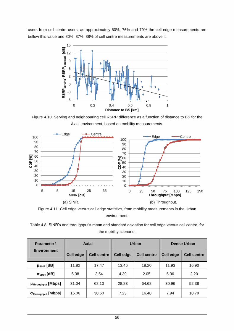
56
users from cell centre users, as approximately 80%, 76% and 79% the cell edge measurements are
bellow this value and 80%, 87%, 88% of cell centre measurements are above it.
Figure 4.10. Serving and neighbouring cell RSRP difference as a function of distance to BS for the
Axial environment, based on mobility measurements.
(a) SINR. (b) Throughput.
Figure 4.11. Cell edge versus cell edge statistics, from mobility measurements in the Urban
environment.
Table 4.8. SINR‟s and throughput‟s mean and standard deviation for cell edge versus cell centre, for
the mobility scenario.
Parameter \
Environment
Axial Urban Dense Urban
Cell edge Cell centre Cell edge Cell centre Cell edge Cell centre
µSINR [dB] 11.82 17.47 13.46 18.20 11.93 16.90
σSINR [dB] 5.38 3.54 4.39 2.05 5.36 2.20
µThroughput [Mbps] 31.04 68.10 28.83 64.68 30.96 52.38
σThroughput [Mbps] 16.06 30.60 7.23 16.40 7.94 10.79
-6
-3
0
3
6
9
12
15
0 0.2 0.4 0.6 0.8 1
RS
RP
serv
ing-
RS
RP
de
tecte
d[d
B]
Distance to BS [km]
-5 5 15 25 35
0
10
20
30
40
50
60
70
80
90
100
SINR [dB]
CD
F [
%]
Edge Centre
0 25 50 75 100 125 150
0
10
20
30
40
50
60
70
80
90
100
Throughput [Mbps]
CD
F [
%]
Edge Centre
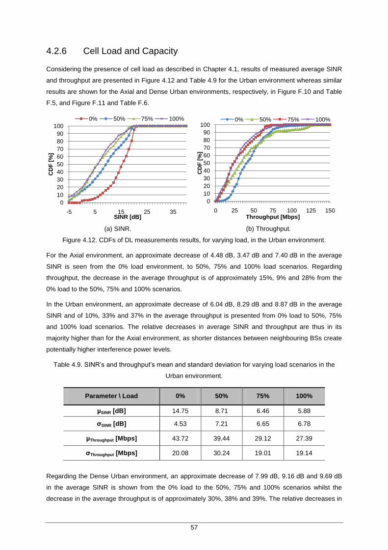
57
4.2.6 Cell Load and Capacity
Considering the presence of cell load as described in Chapter 4.1, results of measured average SINR
and throughput are presented in Figure 4.12 and Table 4.9 for the Urban environment whereas similar
results are shown for the Axial and Dense Urban environments, respectively, in Figure F.10 and Table
F.5, and Figure F.11 and Table F.6.
(a) SINR. (b) Throughput.
Figure 4.12. CDFs of DL measurements results, for varying load, in the Urban environment.
For the Axial environment, an approximate decrease of 4.48 dB, 3.47 dB and 7.40 dB in the average
SINR is seen from the 0% load environment, to 50%, 75% and 100% load scenarios. Regarding
throughput, the decrease in the average throughput is of approximately 15%, 9% and 28% from the
0% load to the 50%, 75% and 100% scenarios.
In the Urban environment, an approximate decrease of 6.04 dB, 8.29 dB and 8.87 dB in the average
SINR and of 10%, 33% and 37% in the average throughput is presented from 0% load to 50%, 75%
and 100% load scenarios. The relative decreases in average SINR and throughput are thus in its
majority higher than for the Axial environment, as shorter distances between neighbouring BSs create
potentially higher interference power levels.
Table 4.9. SINR‟s and throughput‟s mean and standard deviation for varying load scenarios in the
Urban environment.
Parameter \ Load 0% 50% 75% 100%
µSINR [dB] 14.75 8.71 6.46 5.88
σSINR [dB] 4.53 7.21 6.65 6.78
µThroughput [Mbps] 43.72 39.44 29.12 27.39
σThroughput [Mbps] 20.08 30.24 19.01 19.14
Regarding the Dense Urban environment, an approximate decrease of 7.99 dB, 9.16 dB and 9.69 dB
in the average SINR is shown from the 0% load to the 50%, 75% and 100% scenarios whilst the
decrease in the average throughput is of approximately 30%, 38% and 39%. The relative decreases in
-5 5 15 25 35
0
10
20
30
40
50
60
70
80
90
100
SINR [dB]
CD
F [
%]
0% 50% 75% 100%
0 25 50 75 100 125 150
0
10
20
30
40
50
60
70
80
90
100
Throughput [Mbps]
CD
F [
%]
0% 50% 75% 100%
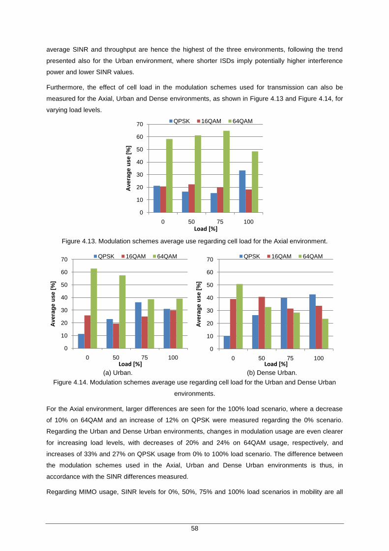
58
average SINR and throughput are hence the highest of the three environments, following the trend
presented also for the Urban environment, where shorter ISDs imply potentially higher interference
power and lower SINR values.
Furthermore, the effect of cell load in the modulation schemes used for transmission can also be
measured for the Axial, Urban and Dense environments, as shown in Figure 4.13 and Figure 4.14, for
varying load levels.
Figure 4.13. Modulation schemes average use regarding cell load for the Axial environment.
(a) Urban. (b) Dense Urban.
Figure 4.14. Modulation schemes average use regarding cell load for the Urban and Dense Urban
environments.
For the Axial environment, larger differences are seen for the 100% load scenario, where a decrease
of 10% on 64QAM and an increase of 12% on QPSK were measured regarding the 0% scenario.
Regarding the Urban and Dense Urban environments, changes in modulation usage are even clearer
for increasing load levels, with decreases of 20% and 24% on 64QAM usage, respectively, and
increases of 33% and 27% on QPSK usage from 0% to 100% load scenario. The difference between
the modulation schemes used in the Axial, Urban and Dense Urban environments is thus, in
accordance with the SINR differences measured.
Regarding MIMO usage, SINR levels for 0%, 50%, 75% and 100% load scenarios in mobility are all
0
10
20
30
40
50
60
70
0 50 75 100
Ave
rag
e u
se
[%
]
Load [%]
QPSK 16QAM 64QAM
0
10
20
30
40
50
60
70
0 50 75 100
Ave
rag
e u
se
[%
]
Load [%]
QPSK 16QAM 64QAM
0
10
20
30
40
50
60
70
0 50 75 100
Ave
rag
e u
se
[%
]
Load [%]
QPSK 16QAM 64QAM
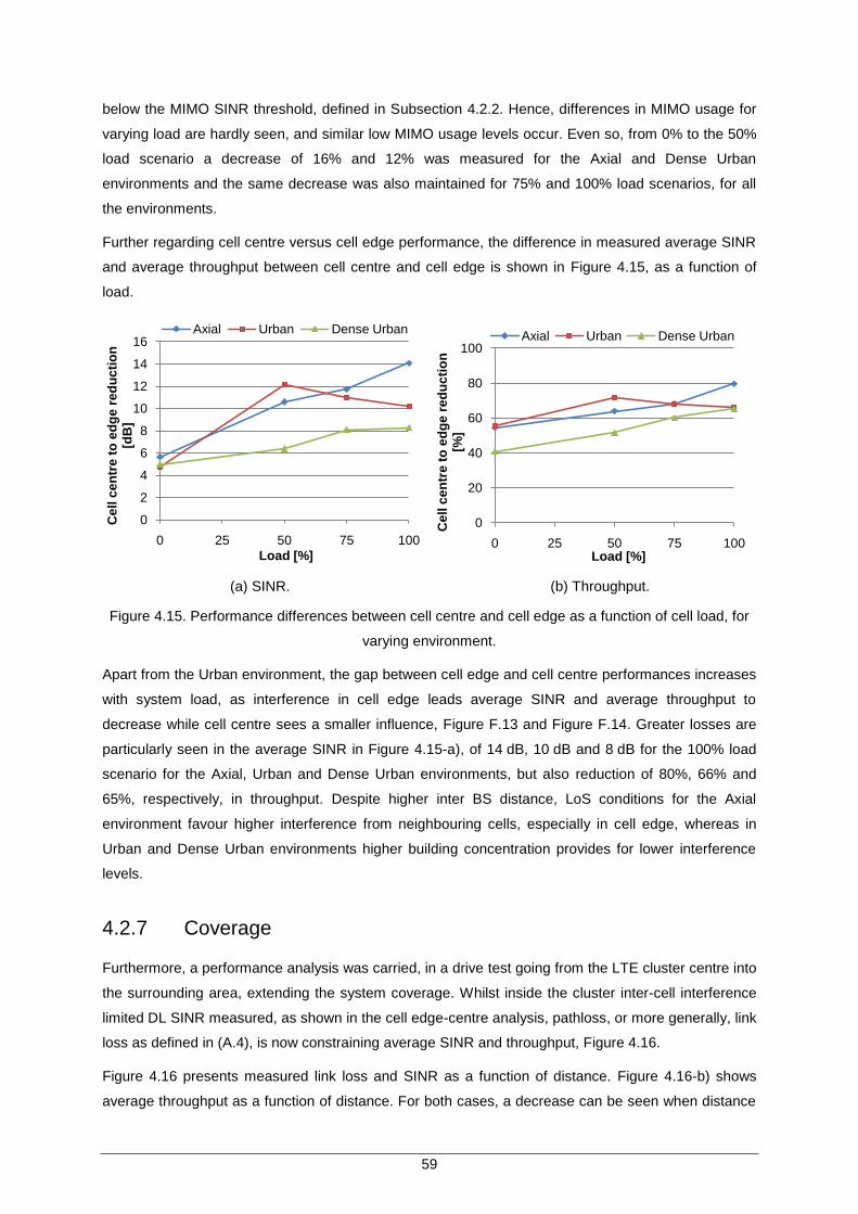
59
below the MIMO SINR threshold, defined in Subsection 4.2.2. Hence, differences in MIMO usage for
varying load are hardly seen, and similar low MIMO usage levels occur. Even so, from 0% to the 50%
load scenario a decrease of 16% and 12% was measured for the Axial and Dense Urban
environments and the same decrease was also maintained for 75% and 100% load scenarios, for all
the environments.
Further regarding cell centre versus cell edge performance, the difference in measured average SINR
and average throughput between cell centre and cell edge is shown in Figure 4.15, as a function of
load.
(a) SINR. (b) Throughput.
Figure 4.15. Performance differences between cell centre and cell edge as a function of cell load, for
varying environment.
Apart from the Urban environment, the gap between cell edge and cell centre performances increases
with system load, as interference in cell edge leads average SINR and average throughput to
decrease while cell centre sees a smaller influence, Figure F.13 and Figure F.14. Greater losses are
particularly seen in the average SINR in Figure 4.15-a), of 14 dB, 10 dB and 8 dB for the 100% load
scenario for the Axial, Urban and Dense Urban environments, but also reduction of 80%, 66% and
65%, respectively, in throughput. Despite higher inter BS distance, LoS conditions for the Axial
environment favour higher interference from neighbouring cells, especially in cell edge, whereas in
Urban and Dense Urban environments higher building concentration provides for lower interference
levels.
4.2.7 Coverage
Furthermore, a performance analysis was carried, in a drive test going from the LTE cluster centre into
the surrounding area, extending the system coverage. Whilst inside the cluster inter-cell interference
limited DL SINR measured, as shown in the cell edge-centre analysis, pathloss, or more generally, link
loss as defined in (A.4), is now constraining average SINR and throughput, Figure 4.16.
Figure 4.16 presents measured link loss and SINR as a function of distance. Figure 4.16-b) shows
average throughput as a function of distance. For both cases, a decrease can be seen when distance
0 25 50 75 100
0
2
4
6
8
10
12
14
16
Load [%]
Cell
ce
ntr
e t
o e
dg
e r
ed
uc
tio
n
[dB
]
Axial Urban Dense Urban
0 25 50 75 100
0
20
40
60
80
100
Load [%]
Cell
ce
ntr
e t
o e
dg
e r
ed
uc
tio
n
[%]
Axial Urban Dense Urban
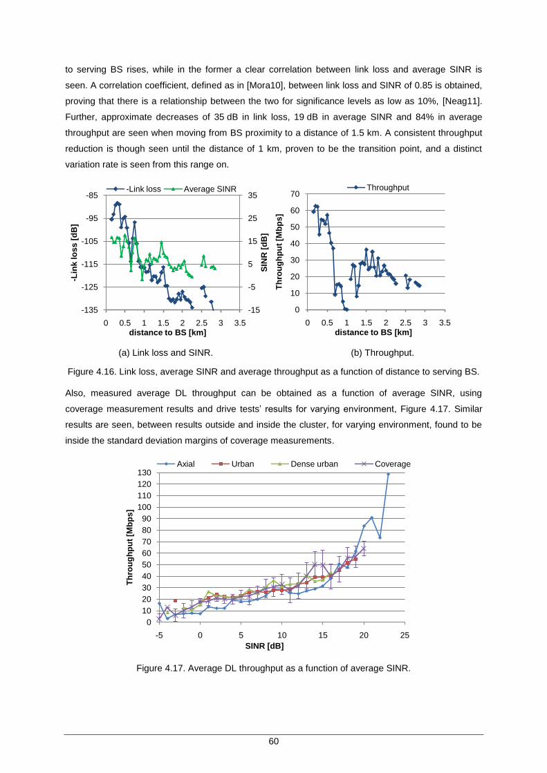
60
to serving BS rises, while in the former a clear correlation between link loss and average SINR is
seen. A correlation coefficient, defined as in [Mora10], between link loss and SINR of 0.85 is obtained,
proving that there is a relationship between the two for significance levels as low as 10%, [Neag11].
Further, approximate decreases of 35 dB in link loss, 19 dB in average SINR and 84% in average
throughput are seen when moving from BS proximity to a distance of 1.5 km. A consistent throughput
reduction is though seen until the distance of 1 km, proven to be the transition point, and a distinct
variation rate is seen from this range on.
(a) Link loss and SINR. (b) Throughput.
Figure 4.16. Link loss, average SINR and average throughput as a function of distance to serving BS.
Also, measured average DL throughput can be obtained as a function of average SINR, using
coverage measurement results and drive tests‟ results for varying environment, Figure 4.17. Similar
results are seen, between results outside and inside the cluster, for varying environment, found to be
inside the standard deviation margins of coverage measurements.
Figure 4.17. Average DL throughput as a function of average SINR.
-15
-5
5
15
25
35
-135
-125
-115
-105
-95
-85
0 0.5 1 1.5 2 2.5 3 3.5
SIN
R [
dB
]
-Lin
k lo
ss
[d
B]
distance to BS [km]
-Link loss Average SINR
0
10
20
30
40
50
60
70
0 0.5 1 1.5 2 2.5 3 3.5
Th
rou
gh
pu
t [M
bp
s]
distance to BS [km]
Throughput
0
10
20
30
40
50
60
70
80
90
100
110
120
130
-5 0 5 10 15 20 25
Th
rou
gh
pu
t [M
bp
s]
SINR [dB]
Axial Urban Dense urban Coverage
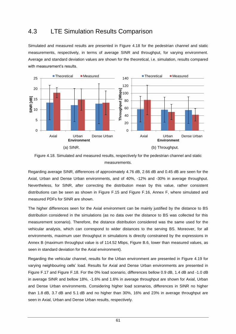
61
4.3 LTE Simulation Results Comparison
Simulated and measured results are presented in Figure 4.18 for the pedestrian channel and static
measurements, respectively, in terms of average SINR and throughput, for varying environment.
Average and standard deviation values are shown for the theoretical, i.e. simulation, results compared
with measurement‟s results.
(a) SINR. (b) Throughput.
Figure 4.18. Simulated and measured results, respectively for the pedestrian channel and static
measurements.
Regarding average SINR, differences of approximately 4.76 dB, 2.66 dB and 0.45 dB are seen for the
Axial, Urban and Dense Urban environments, and of 40%, -12% and -30% in average throughput.
Nevertheless, for SINR, after correcting the distribution mean by this value, rather consistent
distributions can be seen as shown in Figure F.15 and Figure F.16, Annex F, where simulated and
measured PDFs for SINR are shown.
The higher differences seen for the Axial environment can be mainly justified by the distance to BS
distribution considered in the simulations (as no data over the distance to BS was collected for this
measurement scenario). Therefore, the distance distribution considered was the same used for the
vehicular analysis, which can correspond to wider distances to the serving BS. Moreover, for all
environments, maximum user throughput in simulations is directly constrained by the expressions in
Annex B (maximum throughput value is of 114.52 Mbps, Figure B.6, lower than measured values, as
seen in standard deviation for the Axial environment).
Regarding the vehicular channel, results for the Urban environment are presented in Figure 4.19 for
varying neighbouring cells‟ load. Results for Axial and Dense Urban environments are presented in
Figure F.17 and Figure F.18. For the 0% load scenario, differences bellow 0.9 dB, 1.4 dB and -1.0 dB
in average SINR and bellow 18%, -1.6% and 1.6% in average throughput are shown for Axial, Urban
and Dense Urban environments. Considering higher load scenarios, differences in SINR no higher
than 1.8 dB, 3.7 dB and 5.1 dB and no higher than 30%, 16% and 23% in average throughput are
seen in Axial, Urban and Dense Urban results, respectively.
0
5
10
15
20
25
Axial Urban Dense Urban
SIN
R [
dB
]
Environment
Theoretical Measured
0
20
40
60
80
100
120
140
Axial Urban Dense Urban
Th
rou
gh
pu
t [M
bp
s]
Environment
Theoretical Measured
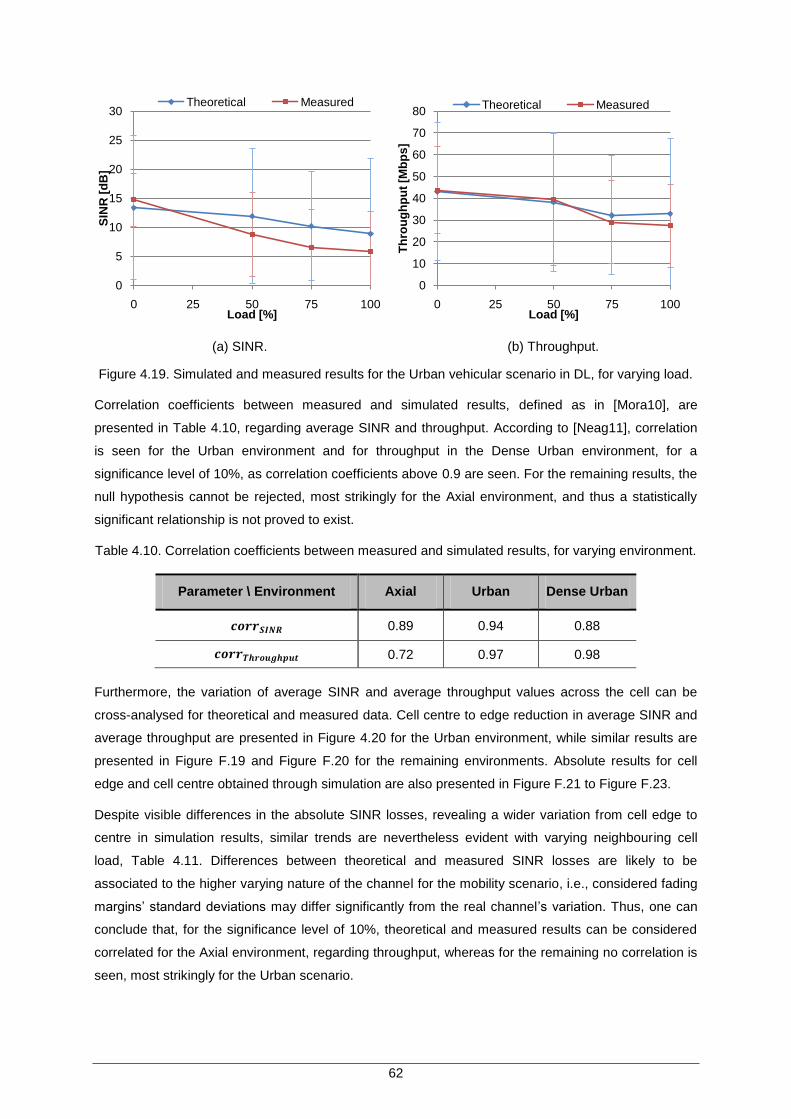
62
(a) SINR. (b) Throughput.
Figure 4.19. Simulated and measured results for the Urban vehicular scenario in DL, for varying load.
Correlation coefficients between measured and simulated results, defined as in [Mora10], are
presented in Table 4.10, regarding average SINR and throughput. According to [Neag11], correlation
is seen for the Urban environment and for throughput in the Dense Urban environment, for a
significance level of 10%, as correlation coefficients above 0.9 are seen. For the remaining results, the
null hypothesis cannot be rejected, most strikingly for the Axial environment, and thus a statistically
significant relationship is not proved to exist.
Table 4.10. Correlation coefficients between measured and simulated results, for varying environment.
Parameter \ Environment Axial Urban Dense Urban
0.89 0.94 0.88
0.72 0.97 0.98
Furthermore, the variation of average SINR and average throughput values across the cell can be
cross-analysed for theoretical and measured data. Cell centre to edge reduction in average SINR and
average throughput are presented in Figure 4.20 for the Urban environment, while similar results are
presented in Figure F.19 and Figure F.20 for the remaining environments. Absolute results for cell
edge and cell centre obtained through simulation are also presented in Figure F.21 to Figure F.23.
Despite visible differences in the absolute SINR losses, revealing a wider variation from cell edge to
centre in simulation results, similar trends are nevertheless evident with varying neighbouring cell
load, Table 4.11. Differences between theoretical and measured SINR losses are likely to be
associated to the higher varying nature of the channel for the mobility scenario, i.e., considered fading
margins‟ standard deviations may differ significantly from the real channel‟s variation. Thus, one can
conclude that, for the significance level of 10%, theoretical and measured results can be considered
correlated for the Axial environment, regarding throughput, whereas for the remaining no correlation is
seen, most strikingly for the Urban scenario.
0
5
10
15
20
25
30
0 25 50 75 100
SIN
R [
dB
]
Load [%]
Theoretical Measured
0
10
20
30
40
50
60
70
80
0 25 50 75 100
Th
rou
gh
pu
t [M
bp
s]
Load [%]
Theoretical Measured
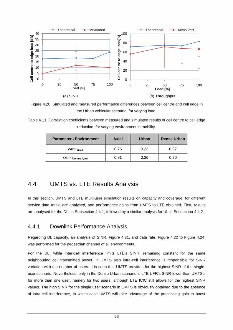
63
(a) SINR. (b) Throughput.
Figure 4.20. Simulated and measured performance differences between cell centre and cell edge in
the Urban vehicular scenario, for varying load.
Table 4.11. Correlation coefficients between measured and simulated results of cell centre to cell edge
reduction, for varying environment in mobility.
Parameter \ Environment Axial Urban Dense Urban
0.76 0.23 0.57
0.91 0.36 0.70
4.4 UMTS vs. LTE Results Analysis
In this section, UMTS and LTE multi-user simulation results on capacity and coverage, for different
service data rates, are analysed, and performance gains from UMTS to LTE obtained. First, results
are analysed for the DL, in Subsection 4.4.1, followed by a similar analysis for UL in Subsection 4.4.2.
4.4.1 Downlink Performance Analysis
Regarding DL capacity, an analysis of SINR, Figure 4.21, and data rate, Figure 4.22 to Figure 4.24,
was performed for the pedestrian channel of all environments.
For the DL, while inter-cell interference limits LTE‟s SINR, remaining constant for the same
neighbouring cell transmitted power, in UMTS also intra-cell interference is responsible for SINR
variation with the number of users. It is seen that UMTS provides for the highest SINR of the single-
user scenario. Nevertheless, only in the Dense Urban scenario is LTE UFR‟s SINR lower than UMTS‟s
for more than one user, namely for two users, although LTE ICIC still allows for the highest SINR
values. The high SINR for the single user scenario in UMTS is obviously obtained due to the absence
of intra-cell interference, in which case UMTS will take advantage of the processing gain to boost
0 25 50 75 100
0
5
10
15
20
25
30
35
40
Load [%]
Ce
ll c
en
tre
to
ed
ge
lo
ss
[d
B]
Theoretical Measured
0 25 50 75 100
0
20
40
60
80
100
Load [%]
Ce
ll c
en
tre
to
ed
ge
lo
ss
[%]
Theoretical Measured
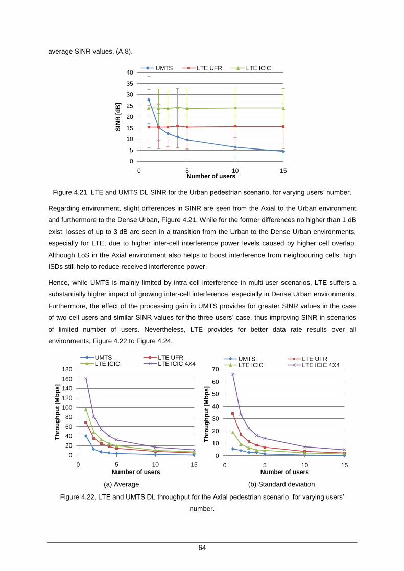
64
average SINR values, (A.8).
Figure 4.21. LTE and UMTS DL SINR for the Urban pedestrian scenario, for varying users‟ number.
Regarding environment, slight differences in SINR are seen from the Axial to the Urban environment
and furthermore to the Dense Urban, Figure 4.21. While for the former differences no higher than 1 dB
exist, losses of up to 3 dB are seen in a transition from the Urban to the Dense Urban environments,
especially for LTE, due to higher inter-cell interference power levels caused by higher cell overlap.
Although LoS in the Axial environment also helps to boost interference from neighbouring cells, high
ISDs still help to reduce received interference power.
Hence, while UMTS is mainly limited by intra-cell interference in multi-user scenarios, LTE suffers a
substantially higher impact of growing inter-cell interference, especially in Dense Urban environments.
Furthermore, the effect of the processing gain in UMTS provides for greater SINR values in the case
of two cell users and similar SINR values for the three users‟ case, thus improving SINR in scenarios
of limited number of users. Nevertheless, LTE provides for better data rate results over all
environments, Figure 4.22 to Figure 4.24.
(a) Average. (b) Standard deviation.
Figure 4.22. LTE and UMTS DL throughput for the Axial pedestrian scenario, for varying users‟
number.
0
5
10
15
20
25
30
35
40
0 5 10 15
SIN
R [
dB
]
Number of users
UMTS LTE UFR LTE ICIC
0
20
40
60
80
100
120
140
160
180
0 5 10 15
Th
rou
gh
pu
t [M
bp
s]
Number of users
UMTS LTE UFRLTE ICIC LTE ICIC 4X4
0
10
20
30
40
50
60
70
0 5 10 15
Th
rou
gh
pu
t [M
bp
s]
Number of users
UMTS LTE UFRLTE ICIC LTE ICIC 4X4
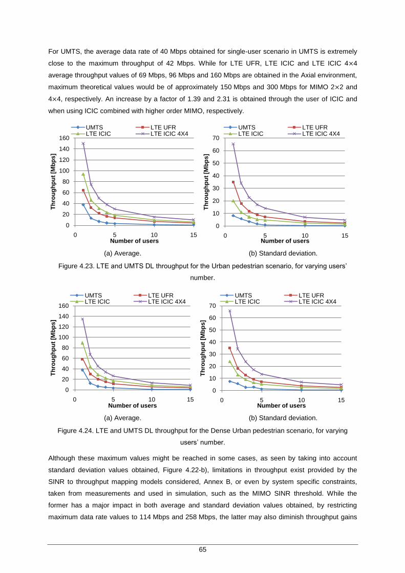
65
For UMTS, the average data rate of 40 Mbps obtained for single-user scenario in UMTS is extremely
close to the maximum throughput of 42 Mbps. While for LTE UFR, LTE ICIC and LTE ICIC 4 4
average throughput values of 69 Mbps, 96 Mbps and 160 Mbps are obtained in the Axial environment,
maximum theoretical values would be of approximately 150 Mbps and 300 Mbps for MIMO 2 2 and
4 4, respectively. An increase by a factor of 1.39 and 2.31 is obtained through the user of ICIC and
when using ICIC combined with higher order MIMO, respectively.
(a) Average. (b) Standard deviation.
Figure 4.23. LTE and UMTS DL throughput for the Urban pedestrian scenario, for varying users‟
number.
(a) Average. (b) Standard deviation.
Figure 4.24. LTE and UMTS DL throughput for the Dense Urban pedestrian scenario, for varying
users‟ number.
Although these maximum values might be reached in some cases, as seen by taking into account
standard deviation values obtained, Figure 4.22-b), limitations in throughput exist provided by the
SINR to throughput mapping models considered, Annex B, or even by system specific constraints,
taken from measurements and used in simulation, such as the MIMO SINR threshold. While the
former has a major impact in both average and standard deviation values obtained, by restricting
maximum data rate values to 114 Mbps and 258 Mbps, the latter may also diminish throughput gains
0
20
40
60
80
100
120
140
160
0 5 10 15
Th
rou
gh
pu
t [M
bp
s]
Number of users
UMTS LTE UFRLTE ICIC LTE ICIC 4X4
0
10
20
30
40
50
60
70
0 5 10 15
Th
rou
gh
pu
t [M
bp
s]
Number of users
UMTS LTE UFRLTE ICIC LTE ICIC 4X4
0
20
40
60
80
100
120
140
160
0 5 10 15
Th
rou
gh
pu
t [M
bp
s]
Number of users
UMTS LTE UFRLTE ICIC LTE ICIC 4X4
0
10
20
30
40
50
60
70
0 5 10 15
Th
rou
gh
pu
t [M
bp
s]
Number of users
UMTS LTE UFRLTE ICIC LTE ICIC 4X4
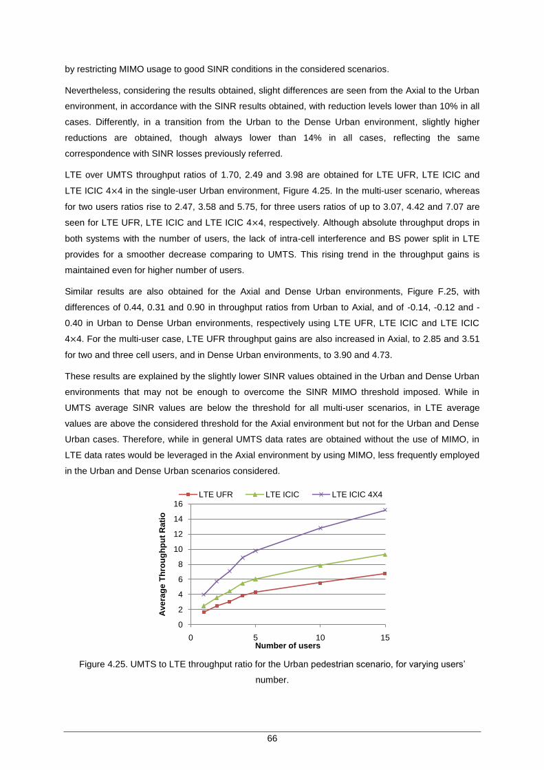
66
by restricting MIMO usage to good SINR conditions in the considered scenarios.
Nevertheless, considering the results obtained, slight differences are seen from the Axial to the Urban
environment, in accordance with the SINR results obtained, with reduction levels lower than 10% in all
cases. Differently, in a transition from the Urban to the Dense Urban environment, slightly higher
reductions are obtained, though always lower than 14% in all cases, reflecting the same
correspondence with SINR losses previously referred.
LTE over UMTS throughput ratios of 1.70, 2.49 and 3.98 are obtained for LTE UFR, LTE ICIC and
LTE ICIC 4 4 in the single-user Urban environment, Figure 4.25. In the multi-user scenario, whereas
for two users ratios rise to 2.47, 3.58 and 5.75, for three users ratios of up to 3.07, 4.42 and 7.07 are
seen for LTE UFR, LTE ICIC and LTE ICIC 4 4, respectively. Although absolute throughput drops in
both systems with the number of users, the lack of intra-cell interference and BS power split in LTE
provides for a smoother decrease comparing to UMTS. This rising trend in the throughput gains is
maintained even for higher number of users.
Similar results are also obtained for the Axial and Dense Urban environments, Figure F.25, with
differences of 0.44, 0.31 and 0.90 in throughput ratios from Urban to Axial, and of -0.14, -0.12 and -
0.40 in Urban to Dense Urban environments, respectively using LTE UFR, LTE ICIC and LTE ICIC
4 4. For the multi-user case, LTE UFR throughput gains are also increased in Axial, to 2.85 and 3.51
for two and three cell users, and in Dense Urban environments, to 3.90 and 4.73.
These results are explained by the slightly lower SINR values obtained in the Urban and Dense Urban
environments that may not be enough to overcome the SINR MIMO threshold imposed. While in
UMTS average SINR values are below the threshold for all multi-user scenarios, in LTE average
values are above the considered threshold for the Axial environment but not for the Urban and Dense
Urban cases. Therefore, while in general UMTS data rates are obtained without the use of MIMO, in
LTE data rates would be leveraged in the Axial environment by using MIMO, less frequently employed
in the Urban and Dense Urban scenarios considered.
Figure 4.25. UMTS to LTE throughput ratio for the Urban pedestrian scenario, for varying users‟
number.
0
2
4
6
8
10
12
14
16
0 5 10 15
Ave
rag
e T
hro
ug
hp
ut
Rati
o
Number of users
LTE UFR LTE ICIC LTE ICIC 4X4
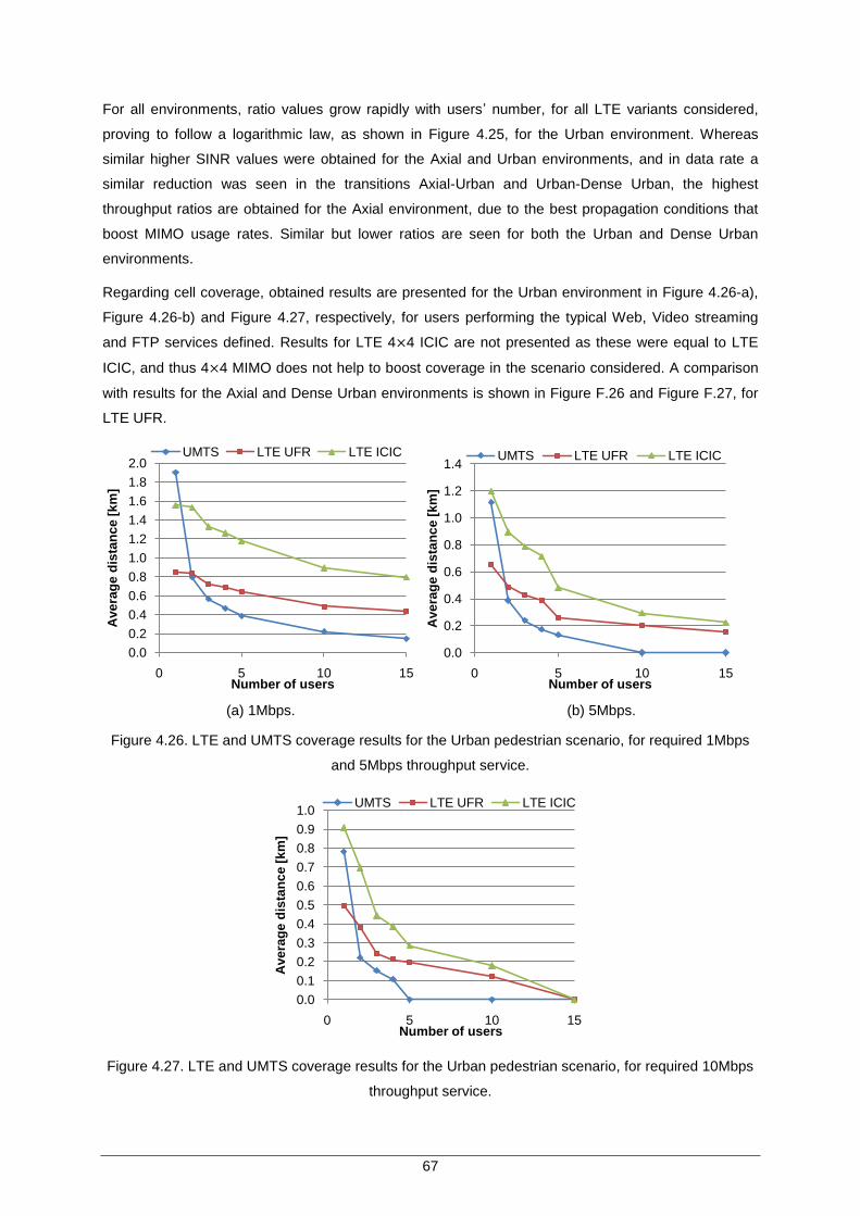
67
For all environments, ratio values grow rapidly with users‟ number, for all LTE variants considered,
proving to follow a logarithmic law, as shown in Figure 4.25, for the Urban environment. Whereas
similar higher SINR values were obtained for the Axial and Urban environments, and in data rate a
similar reduction was seen in the transitions Axial-Urban and Urban-Dense Urban, the highest
throughput ratios are obtained for the Axial environment, due to the best propagation conditions that
boost MIMO usage rates. Similar but lower ratios are seen for both the Urban and Dense Urban
environments.
Regarding cell coverage, obtained results are presented for the Urban environment in Figure 4.26-a),
Figure 4.26-b) and Figure 4.27, respectively, for users performing the typical Web, Video streaming
and FTP services defined. Results for LTE 4 4 ICIC are not presented as these were equal to LTE
ICIC, and thus 4 4 MIMO does not help to boost coverage in the scenario considered. A comparison
with results for the Axial and Dense Urban environments is shown in Figure F.26 and Figure F.27, for
LTE UFR.
(a) 1Mbps. (b) 5Mbps.
Figure 4.26. LTE and UMTS coverage results for the Urban pedestrian scenario, for required 1Mbps
and 5Mbps throughput service.
Figure 4.27. LTE and UMTS coverage results for the Urban pedestrian scenario, for required 10Mbps
throughput service.
0.0
0.2
0.4
0.6
0.8
1.0
1.2
1.4
1.6
1.8
2.0
0 5 10 15
Ave
rag
e d
ista
nc
e [
km
]
Number of users
UMTS LTE UFR LTE ICIC
0.0
0.2
0.4
0.6
0.8
1.0
1.2
1.4
0 5 10 15
Ave
rag
e d
ista
nc
e [
km
]
Number of users
UMTS LTE UFR LTE ICIC
0.0
0.1
0.2
0.3
0.4
0.5
0.6
0.7
0.8
0.9
1.0
0 5 10 15
Ave
rag
e d
ista
nc
e [
km
]
Number of users
UMTS LTE UFR LTE ICIC
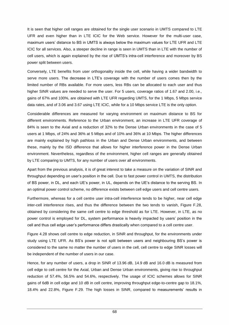
68
It is seen that higher cell ranges are obtained for the single user scenario in UMTS compared to LTE
UFR and even higher than in LTE ICIC for the Web service. However for the multi-user case,
maximum users‟ distance to BS in UMTS is always below the maximum values for LTE UFR and LTE
ICIC for all services. Also, a steeper decline in range is seen in UMTS than in LTE with the number of
cell users, which is again explained by the rise of UMTS‟s intra-cell interference and moreover by BS
power split between users.
Conversely, LTE benefits from user orthogonality inside the cell, while having a wider bandwidth to
serve more users. The decrease in LTE‟s coverage with the number of users comes then by the
limited number of RBs available. For more users, less RBs can be allocated to each user and thus
higher SINR values are needed to serve the user. For 5 users, coverage ratios of 1.67 and 2.00, i.e.,
gains of 67% and 100%, are obtained with LTE UFR regarding UMTS, for the 1 Mbps, 5 Mbps service
data rates, and of 3.06 and 3.67 using LTE ICIC, while for a 10 Mbps service LTE is the only option.
Considerable differences are measured for varying environment on maximum distance to BS for
different environments. Reference to the Urban environment, an increase in LTE UFR coverage of
84% is seen to the Axial and a reduction of 32% to the Dense Urban environments in the case of 5
users at 1 Mbps, of 24% and 36% at 5 Mbps and of 10% and 36% at 10 Mbps. The higher differences
are mainly explained by high pathloss in the Urban and Dense Urban environments, and between
these, mainly by the ISD difference that allows for higher interference power in the Dense Urban
environment. Nevertheless, regardless of the environment, higher cell ranges are generally obtained
by LTE comparing to UMTS, for any number of users over all environments.
Apart from the previous analysis, it is of great interest to take a measure on the variation of SINR and
throughput depending on user‟s position in the cell. Due to fast power control in UMTS, the distribution
of BS power, in DL, and each UE‟s power, in UL, depends on the UE‟s distance to the serving BS. In
an optimal power control scheme, no difference exists between cell edge users and cell centre users.
Furthermore, whereas for a cell centre user intra-cell interference tends to be higher, near cell edge
inter-cell interference rises, and thus the difference between the two tends to vanish, Figure F.28,
obtained by considering the same cell centre to edge threshold as for LTE. However, in LTE, as no
power control is employed for DL, system performance is heavily impacted by users‟ position in the
cell and thus cell edge user‟s performance differs drastically when compared to a cell centre user.
Figure 4.28 shows cell centre to edge reduction, in SINR and throughput, for the environments under
study using LTE UFR. As BS‟s power is not split between users and neighbouring BS‟s power is
considered to the same no matter the number of users in the cell, cell centre to edge SINR losses will
be independent of the number of users in our case.
Hence, for any number of users, a drop in SINR of 13.96 dB, 14.9 dB and 16.0 dB is measured from
cell edge to cell centre for the Axial, Urban and Dense Urban environments, giving rise to throughput
reduction of 57.4%, 56.5% and 54.6%, respectively. The usage of ICIC schemes allows for SINR
gains of 6dB in cell edge and 10 dB in cell centre, improving throughput edge-to-centre gap to 18.1%,
18.4% and 22.8%, Figure F.29. The high losses in SINR, compared to measurements‟ results in
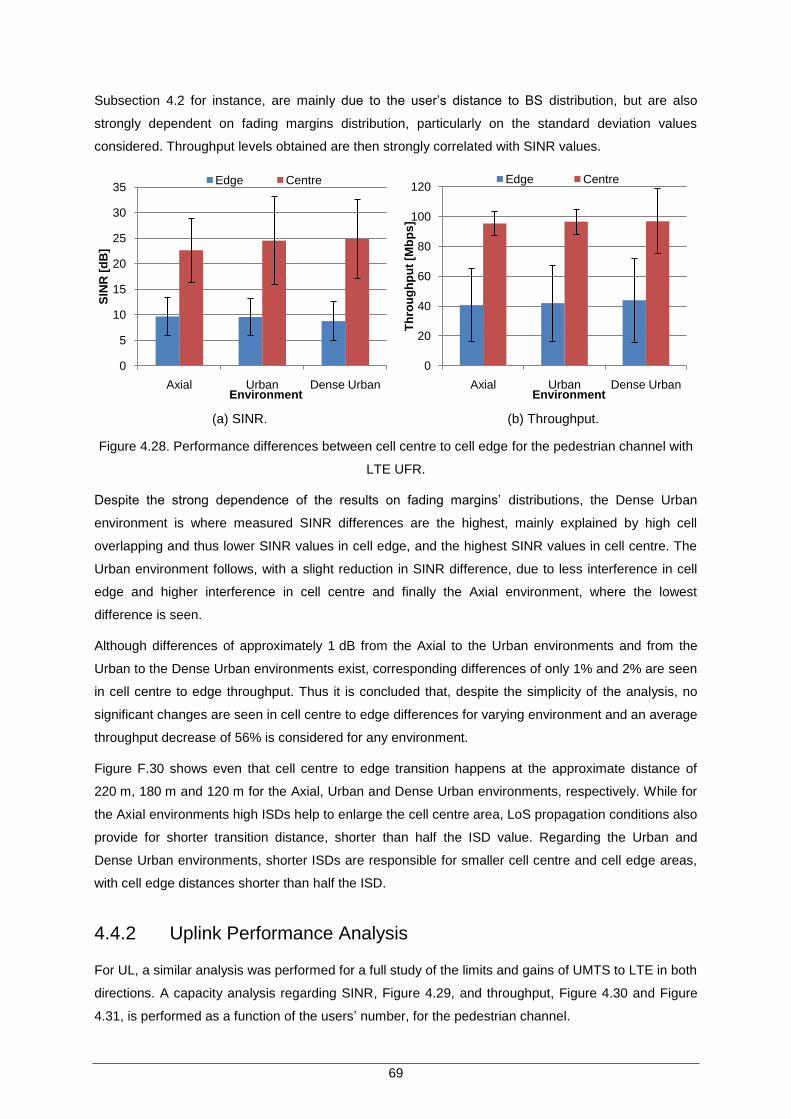
69
Subsection 4.2 for instance, are mainly due to the user‟s distance to BS distribution, but are also
strongly dependent on fading margins distribution, particularly on the standard deviation values
considered. Throughput levels obtained are then strongly correlated with SINR values.
(a) SINR. (b) Throughput.
Figure 4.28. Performance differences between cell centre to cell edge for the pedestrian channel with
LTE UFR.
Despite the strong dependence of the results on fading margins‟ distributions, the Dense Urban
environment is where measured SINR differences are the highest, mainly explained by high cell
overlapping and thus lower SINR values in cell edge, and the highest SINR values in cell centre. The
Urban environment follows, with a slight reduction in SINR difference, due to less interference in cell
edge and higher interference in cell centre and finally the Axial environment, where the lowest
difference is seen.
Although differences of approximately 1 dB from the Axial to the Urban environments and from the
Urban to the Dense Urban environments exist, corresponding differences of only 1% and 2% are seen
in cell centre to edge throughput. Thus it is concluded that, despite the simplicity of the analysis, no
significant changes are seen in cell centre to edge differences for varying environment and an average
throughput decrease of 56% is considered for any environment.
Figure F.30 shows even that cell centre to edge transition happens at the approximate distance of
220 m, 180 m and 120 m for the Axial, Urban and Dense Urban environments, respectively. While for
the Axial environments high ISDs help to enlarge the cell centre area, LoS propagation conditions also
provide for shorter transition distance, shorter than half the ISD value. Regarding the Urban and
Dense Urban environments, shorter ISDs are responsible for smaller cell centre and cell edge areas,
with cell edge distances shorter than half the ISD.
4.4.2 Uplink Performance Analysis
For UL, a similar analysis was performed for a full study of the limits and gains of UMTS to LTE in both
directions. A capacity analysis regarding SINR, Figure 4.29, and throughput, Figure 4.30 and Figure
4.31, is performed as a function of the users‟ number, for the pedestrian channel.
0
5
10
15
20
25
30
35
Axial Urban Dense Urban
SIN
R [
dB
]
Environment
Edge Centre
0
20
40
60
80
100
120
Axial Urban Dense Urban
Th
rou
gh
pu
t [M
bp
s]
Environment
Edge Centre
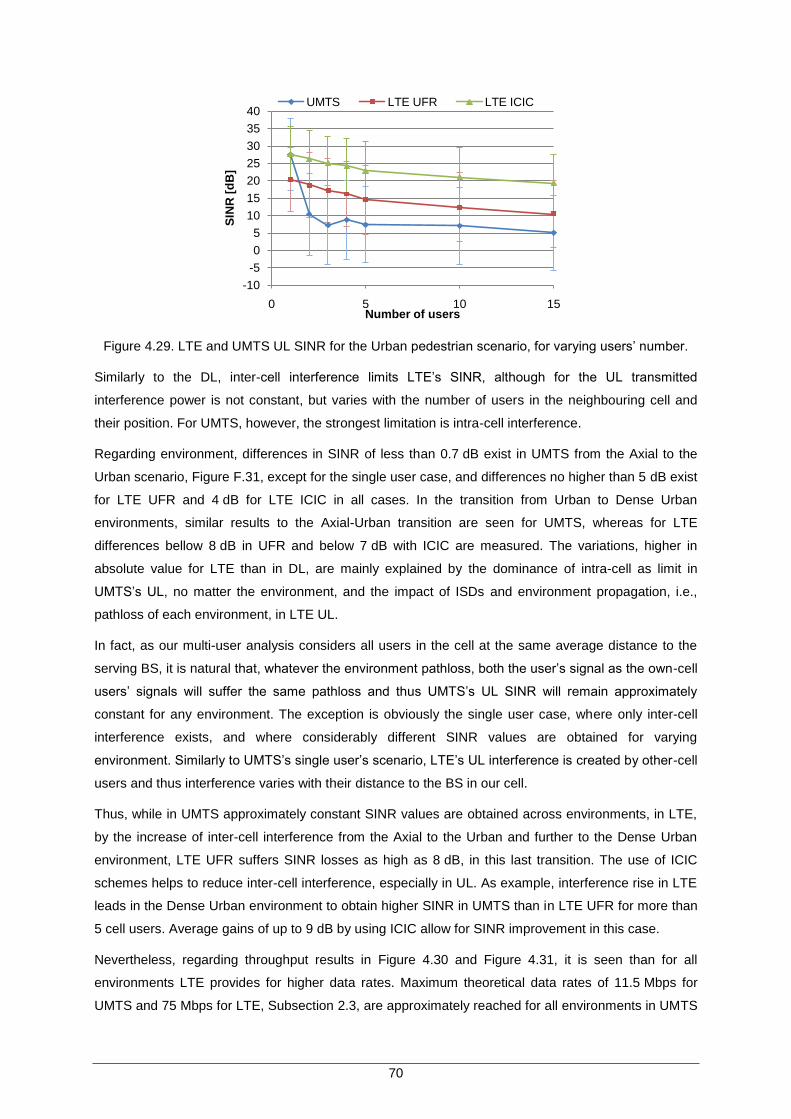
70
Figure 4.29. LTE and UMTS UL SINR for the Urban pedestrian scenario, for varying users‟ number.
Similarly to the DL, inter-cell interference limits LTE‟s SINR, although for the UL transmitted
interference power is not constant, but varies with the number of users in the neighbouring cell and
their position. For UMTS, however, the strongest limitation is intra-cell interference.
Regarding environment, differences in SINR of less than 0.7 dB exist in UMTS from the Axial to the
Urban scenario, Figure F.31, except for the single user case, and differences no higher than 5 dB exist
for LTE UFR and 4 dB for LTE ICIC in all cases. In the transition from Urban to Dense Urban
environments, similar results to the Axial-Urban transition are seen for UMTS, whereas for LTE
differences bellow 8 dB in UFR and below 7 dB with ICIC are measured. The variations, higher in
absolute value for LTE than in DL, are mainly explained by the dominance of intra-cell as limit in
UMTS‟s UL, no matter the environment, and the impact of ISDs and environment propagation, i.e.,
pathloss of each environment, in LTE UL.
In fact, as our multi-user analysis considers all users in the cell at the same average distance to the
serving BS, it is natural that, whatever the environment pathloss, both the user‟s signal as the own-cell
users‟ signals will suffer the same pathloss and thus UMTS‟s UL SINR will remain approximately
constant for any environment. The exception is obviously the single user case, where only inter-cell
interference exists, and where considerably different SINR values are obtained for varying
environment. Similarly to UMTS‟s single user‟s scenario, LTE‟s UL interference is created by other-cell
users and thus interference varies with their distance to the BS in our cell.
Thus, while in UMTS approximately constant SINR values are obtained across environments, in LTE,
by the increase of inter-cell interference from the Axial to the Urban and further to the Dense Urban
environment, LTE UFR suffers SINR losses as high as 8 dB, in this last transition. The use of ICIC
schemes helps to reduce inter-cell interference, especially in UL. As example, interference rise in LTE
leads in the Dense Urban environment to obtain higher SINR in UMTS than in LTE UFR for more than
5 cell users. Average gains of up to 9 dB by using ICIC allow for SINR improvement in this case.
Nevertheless, regarding throughput results in Figure 4.30 and Figure 4.31, it is seen than for all
environments LTE provides for higher data rates. Maximum theoretical data rates of 11.5 Mbps for
UMTS and 75 Mbps for LTE, Subsection 2.3, are approximately reached for all environments in UMTS
-10
-5
0
5
10
15
20
25
30
35
40
0 5 10 15
SIN
R [
dB
]
Number of users
UMTS LTE UFR LTE ICIC
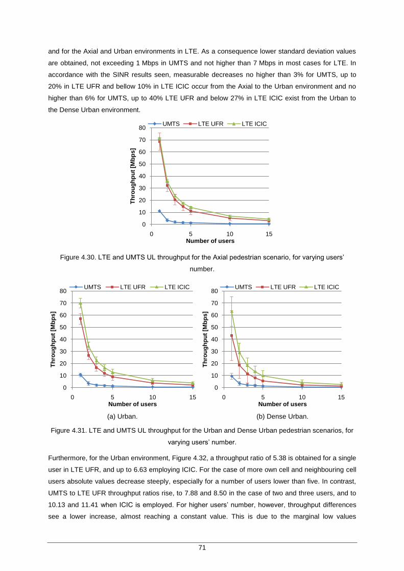
71
and for the Axial and Urban environments in LTE. As a consequence lower standard deviation values
are obtained, not exceeding 1 Mbps in UMTS and not higher than 7 Mbps in most cases for LTE. In
accordance with the SINR results seen, measurable decreases no higher than 3% for UMTS, up to
20% in LTE UFR and bellow 10% in LTE ICIC occur from the Axial to the Urban environment and no
higher than 6% for UMTS, up to 40% LTE UFR and below 27% in LTE ICIC exist from the Urban to
the Dense Urban environment.
Figure 4.30. LTE and UMTS UL throughput for the Axial pedestrian scenario, for varying users‟
number.
(a) Urban. (b) Dense Urban.
Figure 4.31. LTE and UMTS UL throughput for the Urban and Dense Urban pedestrian scenarios, for
varying users‟ number.
Furthermore, for the Urban environment, Figure 4.32, a throughput ratio of 5.38 is obtained for a single
user in LTE UFR, and up to 6.63 employing ICIC. For the case of more own cell and neighbouring cell
users absolute values decrease steeply, especially for a number of users lower than five. In contrast,
UMTS to LTE UFR throughput ratios rise, to 7.88 and 8.50 in the case of two and three users, and to
10.13 and 11.41 when ICIC is employed. For higher users‟ number, however, throughput differences
see a lower increase, almost reaching a constant value. This is due to the marginal low values
0
10
20
30
40
50
60
70
80
0 5 10 15
Th
rou
gh
pu
t [M
bp
s]
Number of users
UMTS LTE UFR LTE ICIC
0
10
20
30
40
50
60
70
80
0 5 10 15
Th
rou
gh
pu
t [M
bp
s]
Number of users
UMTS LTE UFR LTE ICIC
0
10
20
30
40
50
60
70
80
0 5 10 15
Th
rou
gh
pu
t [M
bp
s]
Number of users
UMTS LTE UFR LTE ICIC
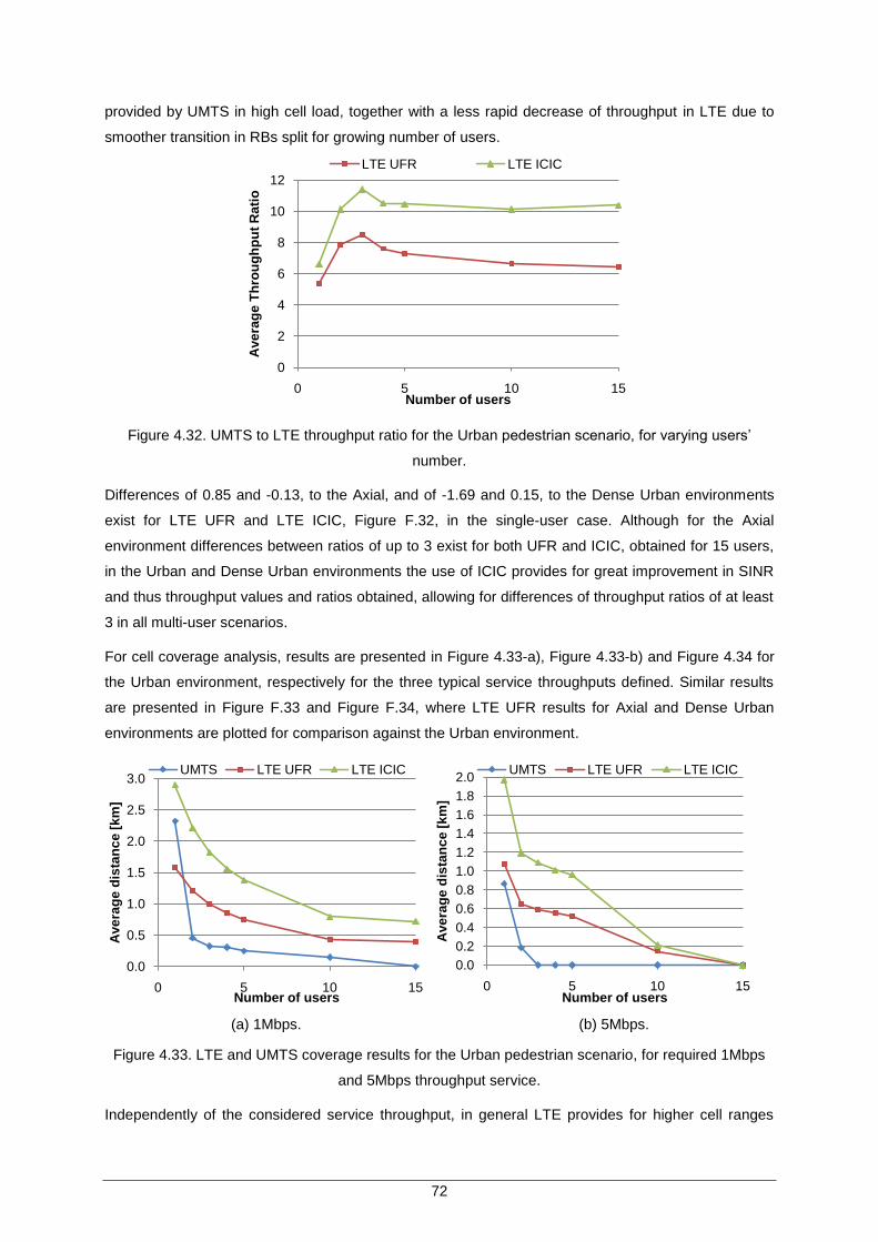
72
provided by UMTS in high cell load, together with a less rapid decrease of throughput in LTE due to
smoother transition in RBs split for growing number of users.
Figure 4.32. UMTS to LTE throughput ratio for the Urban pedestrian scenario, for varying users‟
number.
Differences of 0.85 and -0.13, to the Axial, and of -1.69 and 0.15, to the Dense Urban environments
exist for LTE UFR and LTE ICIC, Figure F.32, in the single-user case. Although for the Axial
environment differences between ratios of up to 3 exist for both UFR and ICIC, obtained for 15 users,
in the Urban and Dense Urban environments the use of ICIC provides for great improvement in SINR
and thus throughput values and ratios obtained, allowing for differences of throughput ratios of at least
3 in all multi-user scenarios.
For cell coverage analysis, results are presented in Figure 4.33-a), Figure 4.33-b) and Figure 4.34 for
the Urban environment, respectively for the three typical service throughputs defined. Similar results
are presented in Figure F.33 and Figure F.34, where LTE UFR results for Axial and Dense Urban
environments are plotted for comparison against the Urban environment.
(a) 1Mbps. (b) 5Mbps.
Figure 4.33. LTE and UMTS coverage results for the Urban pedestrian scenario, for required 1Mbps
and 5Mbps throughput service.
Independently of the considered service throughput, in general LTE provides for higher cell ranges
0
2
4
6
8
10
12
0 5 10 15
Ave
rag
e T
hro
ug
hp
ut
Ra
tio
Number of users
LTE UFR LTE ICIC
0.0
0.5
1.0
1.5
2.0
2.5
3.0
0 5 10 15
Ave
rag
e d
ista
nc
e [
km
]
Number of users
UMTS LTE UFR LTE ICIC
0.0
0.2
0.4
0.6
0.8
1.0
1.2
1.4
1.6
1.8
2.0
0 5 10 15
Ave
rag
e d
ista
nc
e [
km
]
Number of users
UMTS LTE UFR LTE ICIC
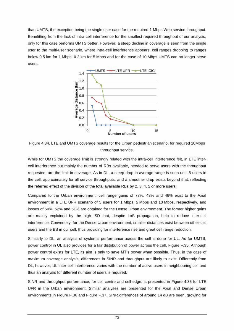
73
than UMTS, the exception being the single user case for the required 1 Mbps Web service throughput.
Benefitting from the lack of intra-cell interference for the smallest required throughput of our analysis,
only for this case performs UMTS better. However, a steep decline in coverage is seen from the single
user to the multi-user scenario, where intra-cell interference appears, cell ranges dropping to ranges
below 0.5 km for 1 Mbps, 0.2 km for 5 Mbps and for the case of 10 Mbps UMTS can no longer serve
users.
Figure 4.34. LTE and UMTS coverage results for the Urban pedestrian scenario, for required 10Mbps
throughput service.
While for UMTS the coverage limit is strongly related with the intra-cell interference felt, in LTE inter-
cell interference but mainly the number of RBs available, needed to serve users with the throughput
requested, are the limit in coverage. As in DL, a steep drop in average range is seen until 5 users in
the cell, approximately for all service throughputs, and a smoother drop exists beyond that, reflecting
the referred effect of the division of the total available RBs by 2, 3, 4, 5 or more users.
Compared to the Urban environment, cell range gains of 77%, 43% and 46% exist to the Axial
environment in a LTE UFR scenario of 5 users for 1 Mbps, 5 Mbps and 10 Mbps, respectively, and
losses of 50%, 52% and 51% are obtained for the Dense Urban environment. The former higher gains
are mainly explained by the high ISD that, despite LoS propagation, help to reduce inter-cell
interference. Conversely, for the Dense Urban environment, smaller distances exist between other-cell
users and the BS in our cell, thus providing for interference rise and great cell range reduction.
Similarly to DL, an analysis of system‟s performance across the cell is done for UL. As for UMTS,
power control in UL also provides for a fair distribution of power across the cell, Figure F.35. Although
power control exists for LTE, its aim is only to save MT‟s power when possible. Thus, in the case of
maximum coverage analysis, differences in SINR and throughput are likely to exist. Differently from
DL, however, UL inter-cell interference varies with the number of active users in neighbouring cell and
thus an analysis for different number of users is required.
SINR and throughput performance, for cell centre and cell edge, is presented in Figure 4.35 for LTE
UFR in the Urban environment. Similar analyses are presented for the Axial and Dense Urban
environments in Figure F.36 and Figure F.37. SINR differences of around 14 dB are seen, growing for
0.0
0.2
0.4
0.6
0.8
1.0
1.2
1.4
0 5 10 15
Ave
rag
e d
ista
nc
e [
km
]
Number of users
UMTS LTE UFR LTE ICIC
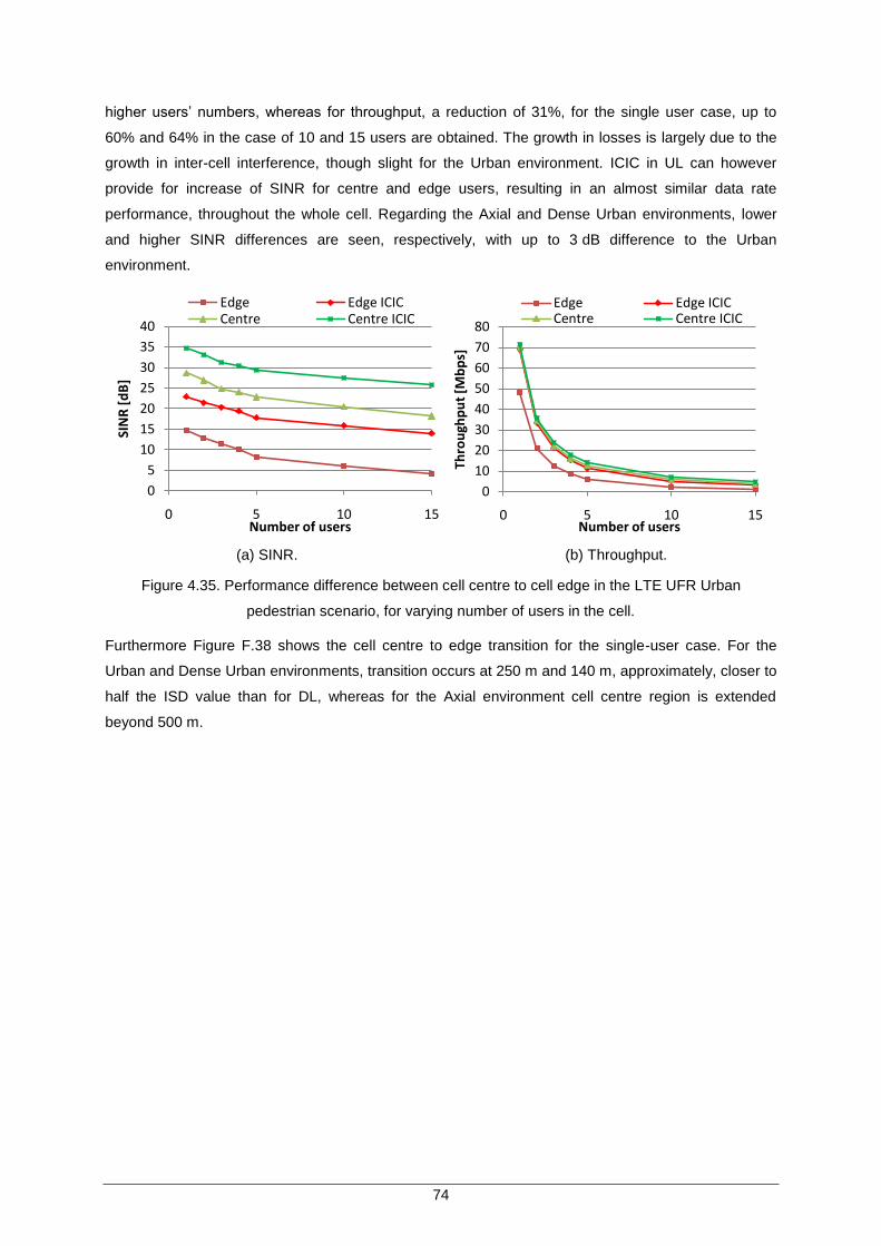
74
higher users‟ numbers, whereas for throughput, a reduction of 31%, for the single user case, up to
60% and 64% in the case of 10 and 15 users are obtained. The growth in losses is largely due to the
growth in inter-cell interference, though slight for the Urban environment. ICIC in UL can however
provide for increase of SINR for centre and edge users, resulting in an almost similar data rate
performance, throughout the whole cell. Regarding the Axial and Dense Urban environments, lower
and higher SINR differences are seen, respectively, with up to 3 dB difference to the Urban
environment.
(a) SINR. (b) Throughput.
Figure 4.35. Performance difference between cell centre to cell edge in the LTE UFR Urban
pedestrian scenario, for varying number of users in the cell.
Furthermore Figure F.38 shows the cell centre to edge transition for the single-user case. For the
Urban and Dense Urban environments, transition occurs at 250 m and 140 m, approximately, closer to
half the ISD value than for DL, whereas for the Axial environment cell centre region is extended
beyond 500 m.
0
5
10
15
20
25
30
35
40
0 5 10 15
SIN
R [
dB
]
Number of users
Edge Edge ICICCentre Centre ICIC
0
10
20
30
40
50
60
70
80
0 5 10 15
Thro
ugh
pu
t [M
bp
s]
Number of users
Edge Edge ICICCentre Centre ICIC
75
Chapter 5
Conclusions
5 Models
This chapter concludes the present dissertation, compiling a discussion and a critical analysis of the
results, presenting the future evolution possibilities of mobile communications, as well as mid-term
future research areas.
76
The main objective of this thesis is to evaluate UMTS/HSPA+ and LTE cellular performance, in terms
of data rate gains, especially regarding capacity and coverage aspects, in different scenarios
regarding channel, environment and the number of users. To accomplish this goal, information was
gathered on both UMTS/HSPA+ and LTE. Higher bandwidth, better spectrum efficiency and more
advanced MIMO schemes allow for higher data rates in LTE than with UMTS, although smoother
performance variation across the cell exists for UMTS.
Based on literature results for both UMTS and LTE, a model was developed and implemented: the
Single Cell model, considering both single- and multi-user scenarios. Two separate components were
considered in the simulator for UMTS and LTE, based on a link budget analysis and literature results
for computing throughput from SINR. COST231-Walfisch-Ikegami propagation model was used to
calculate propagation losses and a channel model was built for computing Rice and Lognormal fading
margins, based on literature studies.
Afterwards, the multi-user approach was considered evolving from the single user one. This extension
to more than one user provides for a more realistic analysis, where different cell load scenarios can be
considered. An important difference from the single to the multi-user scenario is resource sharing,
namely available codes in UMTS and RBs in LTE, and further DL transmission power in UMTS.
Additionally, interference in both systems directly increases with cell load.
Study scenarios were defined, in cooperation with the telecommunications operator Optimus. Axial,
Urban and Dense Urban environments under the pedestrian and vehicular scenarios where
characterised. Further, neighbouring cells load levels were defined for DL, namely by defining BS
transmission power levels. Finally, for the coverage analysis, typical service data rates were defined,
for relevant services described.
A LTE measurements‟ campaign was then conducted in a Portuguese city, where a cluster has been
deployed. DL performance data was collected for the single user case, across the scenarios defined.
Common QPSK, 16QAM and 64QAM modulations were available and up to MIMO 2 2 was possible.
Varying load scenarios were measured. However no ICIC schemes were deployed. The maximum
bandwidth of 20MHz was taken.
Measurements results are analysed regarding varying environment, channel, modulation schemes
and antenna configuration, user positioning in the cell, cell load scenarios and coverage scenarios.
Average throughput values of 82 Mbps, 50 Mbps and 42 Mbps are obtained for static Axial, Urban and
Dense Urban environments, respectively, and of 47 Mbps, 44 Mbps and 39 Mbps for mobility
scenario. For the Axial environment, throughputs are boosted mainly due to MIMO transmission, with
average transmission percentages of 46%, compared to 7% in Urban and 9% in Dense Urban
environments. Static and mobility results are in most cases similar, except for the Axial environment
where measurements spots choices heavily influenced results.
Regarding modulation, 64QAM is the preferred scheme, with 74% average usage over all
environments for the static scenario, followed by 16QAM with 22% and QPSK with 4%. The selection
of HOM schemes is attributed to the lack of load in the system, only used by one user, allowing for low
77
BER levels. Regarding antenna configurations, SINR MIMO thresholds of 16 dB, 17 dB and 16.5 dB
exist for Axial, Urban and Dense Urban environments, above which more than 10% of MIMO usage
occurs.
Users‟ position in the cell is determined to heavily impact obtained data rate, with throughput
reductions of 54%, 55% and 41% measured from cell centre to cell edge in Axial, Urban and Dense
Urban environments, respectively. A cell centre to edge threshold of 15 dB to 16 dB in SINR was
found to exist for all environments measured.
System load, in the form of inter-cell interference, also heavily reduces data rate performance.
Throughput reduction of 10%, 33% and 37% was measured in the Urban environment for 50%, 75%
and 100% load scenarios, regarding the one with 0% load. Similar results were obtained for the
remaining environments. Higher reductions are seen in the Urban compared to the Axial and in the
Dense Urban compared with the Urban environments mainly due to smaller ISDs, higher cell
overlapping and thus higher interference levels.
Furthermore, a reduction in HOM and MIMO usage rates is seen, for rising load, namely due to SINR
reduction. Regarding cell centre to edge transition, data rate reduction tends to increase also for
higher load conditions, with higher difference associated to cell edge users compared to cell centre
ones, due to increase in interference.
Based on measurements‟ results obtained, namely for the same modulation usage distribution and
MIMO SINR threshold for each environment, simulation results were obtained. The same distribution
for user distance to BS, ISD and neighbouring BS power were taken. For both pedestrian and
vehicular channels, results are found to be consistent with static and mobility measurements. Similar
average results are obtained for the former, covered by the measured standard deviation, and
correlation is obtained for the latter, in most cases, for a confidence level of 10%. Nevertheless, higher
standard deviation values are obtained in simulated results, for both the pedestrian and vehicular
channels, suggesting high standard deviation values assumed for the fading margins, mainly
responsible by SINR variation.
Being the simulator validated against measurements results, simulations results were obtained for
UMTS and LTE, for performance comparison. For LTE the deployment of ICIC schemes for UL and
DL and additionally MIMO 4 4 schemes for DL were also considered.
For DL, average 42 Mbps, 69 Mbps, 96 Mbps and 160 Mbps data rates are obtained using UMTS,
LTE UFR, LTE ICIC and LTE ICIC 4 4 and 11 Mbps, 68 Mbps and 72 Mbps using UMTS, LTE UFR,
LTE ICIC for UL in the Axial environment for single-user. High throughputs are mainly explained by
low inter-cell interference existing in this scenario and no intra-cell interference in UMTS. Both for UL
and DL data rates drop rapidly with the number of users. RBs split in LTE and intra-cell interference
rise in UMTS, for UL and DL, and BS power division in UMTS‟s DL justify the performance drop.
Varying environment, decreases in throughput no higher than around 10% exist in DL from the Axial to
Urban and from the Urban to the Axial environments, for both UMTS and LTE, and bellow 6% and
27% in UL, for UMTS and LTE, respectively. Especially for the UL, neighbouring cell users‟ are
78
responsible for steep interference rise in Urban and Dense Urban environments, due to the shortest
ISDs.
DL throughput ratios of 1.73, 2.39 and 4.01 are obtained from UMTS to LTE UFR, LTE ICIC and LTE
ICIC 4 4, for the single-user in the Axial environment. Similar gains are obtained for the Urban and
Dense Urban environments in single user scenario. For increasing number of users, throughput gains
increase rapidly and the highest gains are obtained for the Axial environment, followed by the Urban
and Dense Urban environments. Moreover, average throughput ratio‟s growth in DL proves to follow a
logarithmic law with the number of users, for all analysed environments.
The rapid growth in data rate gains is explained by the increase in intra-cell interference and BS power
split in UMTS, providing for a drop in SINR and hence data rate. Conversely, for LTE, SINR remains
constant for higher number of users, and only the division of available RBs constrains users‟ data
rates. Furthermore, by deploying an ICIC scheme and further using 4 4 MIMO, throughput gains are
significantly improved.
In UL, higher throughput ratios are obtained, of 6.23 and 6.5, respectively employing LTE UFR and
LTE ICIC in the single user Axial scenario. For the multi-user case throughput ratios rise due to intra-
cell interference rise in UMTS, lowering throughputs, and due to a smaller throughput reduction in
LTE, due to RBs split between users. For the Urban environment, a decrease is seen to 5.83 and 6.63
throughput ratios for LTE UFR and LTE ICIC and 4.54 and 6.65 for the Dense Urban. For the multi-
user scenario similar differences are maintained, justified by higher inter-cell interference in Urban and
Dense Urban environments.
Regarding DL coverage, cell ranges of 0.64 km, 0.26 km and 0.20 km are seen with LTE UFR in 5
users‟ Urban scenario, respectively for required 1 Mbps and 5 Mbps 10 Mbps. For UMTS ranges of
0.39 km and 0.13 km, for 1 Mbps and 5 Mbps, are allowed in the same scenario, while for 10 Mbps
users cannot be served. For UL, cell ranges of 0.25 km and 0.75 km are seen with UMTS and LTE
UFR, for serving 5 users at 1 Mbps in the Urban environment, while for higher data rates only LTE is
able to serve all users. Also, for the majority of single- and multi-users scenarios, over all
environments, it is even seen that, for the same throughput, coverage limitations are not imposed by
the UL but by the DL in both systems.
Benefiting from orthogonality inside the cell and a wider bandwidth LTE provides for higher cell ranges
despite higher inter-cell interference comparing to UMTS. Additionally, no BS power split occurs in
LTE DL, which reduces cell range in UMTS for the same power sensitivity.
Moreover, while in UMTS DL cell centre to edge performance tends to be similar by means of power
control, for LTE UFR 56% throughput drops occur from cell centre to cell edge, for the Urban
environment with small differences to the Axial and Dense Urban environments. For UL high losses
are also measured, of approximately 54% and 60% for 5 and 10 cell users. Nevertheless, the centre-
to-edge gap can be significantly reduced by the use of ICIC schemes, to approximately 18% in DL and
to 20% and 27% in UL with 5 and 10 cell users, respectively.
Existing variations in centre-to-edge gap are more significant from the Axial to the Urban and Dense
79
Urban environments and further more in UL than DL namely due to smaller ISDs that boost inter-cell
interference in cell edge. Moreover, while in DL cell centre to edge transition is determined to occur at
the distances 180 m and 120 m respectively for Urban and Dense Urban environments, in UL the
transition occurs at 250 m and 140 m. Thus a greater cell centre region is measured for UL than DL.
All in all, through the analysis of UMTS versus LTE performance it is seen that, apart from very
particular scenarios, higher performance is obtained by the use of LTE especially in the multi-user
case. However, considering different scenarios, e.g. different ISDs, user's distribution in the cell, BS
and MT transmitted powers in cell load and building concentration, results will certainly vary.
As LTE deployment examples start to emerge, and demand for the next generation technology grows,
this thesis is of great practical value. Data rate gains from UMTS to LTE are determined for both
systems and performance aspects analysed, providing for an in depth study across the scenarios of
interest. Furthermore, as LTE presents new challenges at the network management level, gains on
SINR and throughput provided by ICIC and advanced antenna configurations are estimated and
analysed.
Nevertheless, in future work, the impact of varying ICIC schemes should be analysed in more depth,
providing for a more accurate estimation of the gains associated to the different resource managing
schemes and algorithms, both at the cell and network level. The improvement that can be obtained will
have a great impact on the overall LTE system performance, affecting capacity and coverage results.
Similarly, MIMO configurations also boost performance if proper channel conditions are met, and
associated gains for LTE are in need to be studied with a base on real world data, especially for
advanced antenna configurations.
In a more global perspective, end-users are only concerned about having reliant broadband
connection. The use of other solutions such as hybrid UMTS and LTE system with seamless overlay
between the two, UMTS and Wi-Fi, or other combinations that may also make use of WiMAX are of
great interest to the operators, manufacturers and any companies related to the mobile
communications market. The deployment of the next generation systems, converging to a single
platform based on IP, opens a diversity of options carrying different trade-offs between performance
and associated costs, adequate for a variety of distinct case studies.

81
Annex A – Link Budget Annex A – Link Budget
The description in Annex D of COST231-Walfisch-Ikegami was made in the perspective of an outdoor
propagation in the radio link between BS and MT. For indoor cases an extra attenuation could then
added, reflecting building/obstacle penetration, obtaining thus the total attenuation, (A.1).
where:
: pathloss due to outdoor propagation;
: pathloss due to indoor propagation.
(A.1) (A.
1)
The link budget used in this thesis is based on the one on Release 99, as presented in [Jaci09],
adapted to HSPA+ and LTE.
The pathloss can be calculated by:
(A.2) (
A.
2)
where:
: pathloss;
: transmitting power at antenna port;
: transmitting antenna gain;
: available receiving power at antenna port;
: receiving antenna gain.
If diversity is used, is given by:
(A.3) (
B.
2)
where:
:diversity gain.
The diversity gain defined is mainly dependent on the diversity type applied and on the propagation
environment. Typical values stand for 2 or 3 dB for 2 antennas and for SIMO configuration. Assuming
minimally correlated signals, a measure of the maximum values is given by the antenna array, (D.5),
or considering a Maximal Ratio Combining (MRC) scheme, (D.6), taken in this thesis.
Apart from pathloss, also link loss can be defined as:
(A.4) (A.
4)
The Equivalent Isotropic Radiated Power (EIRP) can be calculated for DL by (A.5), and for UL by
(A.6).
82
(A.5) (A.
5)
(A.6) (
A.
6)
where:
: total BS or MT transmission power at the remote radio head output;
: cable losses between transmitter and antenna;
: user losses;
: masthead amplifier gain, being 0 dB in the MU comparison, while in SU is set to 3 dB;
the use of near antenna amplifier provides cable loss compensation and consequent diminish
of noise figure;
: signalling and control power.
SINR can be computed using the results from EIRP and pathloss expressions, respectively for LTE
and HSPA+:
(A.7) (
A.
7)
(A.8) (A.
8)
where:
: total noise power;
: processing gain, equal to 16 for HSPA+ DL and variable for UL.
Specifically for LTE, a SINR gain due to employing an ICIC scheme can be defined:
(A.9) (
A.
9)
where:
: ICIC gain, relative to the scenario with no ICIC, varying depending on user‟s position in
the cell.
Total noise power, defined for the computation of SINR, is given by:
(A.10) (A.10)
where:
: average noise power at the receiver is given by:
(A.11) (B.9)
: interference margin;
: bandwidth of the total RB‟s allocated, while in UMTS equals ;
: noise figure of the receiver.
Alternatively, total interference power can be computed instead of using the interference margin as
given by:
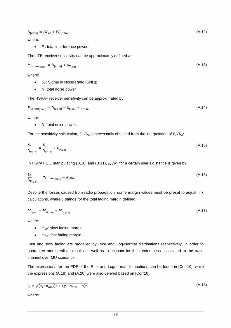
83
(A.12) (A.12)
where:
: total interference power.
The LTE receiver sensitivity can be approximately defined as:
(A.13) (A.13)
where:
: Signal to Noise Ratio (SNR);
: total noise power
The HSPA+ receiver sensitivity can be approximated by:
(A.14) (
A.14)
where:
: total noise power.
For the sensitivity calculation, is necessarily obtained from the interpolation of :
(A.15)
In HSPA+ UL, manipulating (B.10) and (B.11), for a certain user‟s distance is given by:
(A.16)
Despite the losses caused from radio propagation, some margin values must be preset to adjust link
calculations, where (A.17) stands for the total fading margin defined:
(A.17) (
A.17)
where:
: slow fading margin;
: fast fading margin.
Fast and slow fading are modelled by Rice and Log-Normal distributions respectively, in order to
guarantee more realistic results as well as to account for the randomness associated to the radio
channel over MU scenarios.
The expressions for the PDF of the Rice and Lognormal distributions can be found in [Corr10], while
the expressions (A.18) and (A.20) were also derived based on [Corr10]:
(A.18) (A.18)
where:
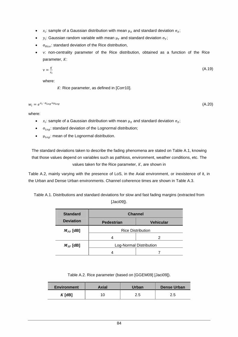
84
: sample of a Gaussian distribution with mean and standard deviation ;
: Gaussian random variable with mean and standard deviation ;
: standard deviation of the Rice distribution,
: non-centrality parameter of the Rice distribution, obtained as a function of the Rice
parameter, :
(A.19) (
A.17)
where:
: Rice parameter, as defined in [Corr10].
(A.20) (A.20)
where:
: sample of a Gaussian distribution with mean and standard deviation ;
: standard deviation of the Lognormal distribution;
: mean of the Lognormal distribution.
The standard deviations taken to describe the fading phenomena are stated on Table A.1, knowing
that those values depend on variables such as pathloss, environment, weather conditions, etc. The
values taken for the Rice parameter, , are shown in
Table A.2, mainly varying with the presence of LoS, in the Axial environment, or inexistence of it, in
the Urban and Dense Urban environments. Channel coherence times are shown in Table A.3.
Table A.1. Distributions and standard deviations for slow and fast fading margins (extracted from
[Jaci09]).
Standard
Deviation
Channel
Pedestrian Vehicular
[dB] Rice Distribution
4 2
[dB] Log-Normal Distribution
4 7
Table A.2. Rice parameter (based on [GGEM09] [Jaci09]).
Environment Axial Urban Dense Urban
[dB] 10 2.5 2.5
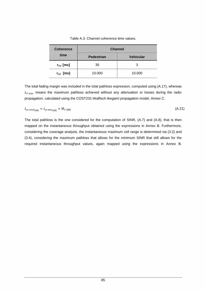
85
Table A.3. Channel coherence time values.
Coherence
time
Channel
Pedestrian Vehicular
[ms] 35 3
[ms] 10.000 10.000
The total fading margin was included in the total pathloss expression, computed using (A.17), whereas
means the maximum pathloss achieved without any attenuation or losses during the radio
propagation, calculated using the COST231-Walfisch-Ikegami propagation model, Annex C.
(A.21) (B.17)
The total pathloss is the one considered for the computation of SINR, (A.7) and (A.8), that is then
mapped on the instantaneous throughput obtained using the expressions in Annex B. Furthermore,
considering the coverage analysis, the instantaneous maximum cell range is determined via (3.2) and
(3.4), considering the maximum pathloss that allows for the minimum SINR that still allows for the
required instantaneous throughput values, again mapped using the expressions in Annex B.

87
Annex B – SINR and Data Rate
Models Annex B – SINR and Data Rate Models
This Annex presents the HSPA+ and LTE models, used to determine SINR and throughput for each
system for several system configurations. The considered models are referred to the throughput over
the physical layer of each system, not considering overhead load and Block Error Rate (BLER).
B.1 UMTS/HSPA+
For UMTS, theoretical throughput values were already presented in Figure 2.2 for a Pedestrian A
channel. Nevertheless, exact expressions are presented to precise SINR, , as a function of
Throughput, , Figure B.1 and Figure B.2, and vice-versa, Figure B.3 and Figure B.4, for several
antenna configuration and modulation schemes, in DL and UL directions. These interpolations were
mainly extracted from [Jaci09] and [Bati11]. Due to the relevance of interference in CDMA systems,
SINR is considered and not SNR.
The results are presented here for a Pedestrian A channel. Due to the relevance of the study of
different radio channels, present in the real environment, different radio channel models should also
be considered. The Vehicular A channel is, in this sense, a usual reference model, and it can be
further be obtained by shifting down the Pedestrian A channel curves presented in 1 dB.
It is worth noticing that the interpolations made bear relative mean errors not greater than 5%,
considered reasonable for this study. Furthermore, the following models consider 15 HS-PDSCH
codes, contrary to the real 14 HS-PDSCH available for traffic, as there were found no results for the
latter number of codes.
Due to lack of suitable data, expressions for QPSK modulation in DL were extrapolated from the ones
for 16QAM, considering the relation between the number of bits per symbol of the two modulation
schemes. Thus, for SISO configuration and QPSK, in DL, SINR is given by the obtained expression:
(B.1)
For SISO configuration and 16QAM, in DL, SINR is given by:
88
(B.2)
For SISO configuration and 64QAM, in DL, one has:
(B.3)
For SIMO 1 2 configuration and QPSK, in DL, SINR is given by:
(B.4)
For SIMO 1 2 configuration and 16QAM, in DL, SINR is given by:
(B.5)
Considering SIMO 1 2 configuration with 64QAM, in DL, SINR is given by;
(B.6)
For MIMO 2 2 using QPSK, in DL, one has:
89
(B.7)
For MIMO 2 2 using 16QAM, in DL, one has:
(B.8)
For a MIMO 2 2 configuration with 64QAM, for DL, SINR is given by:
(B.9)
For QPSK, considering now the UL direction, one has:
(B.10)
Considering 16QAM for UL, the obtained interpolation obtained by (C.8) is shown in Figure B.2.
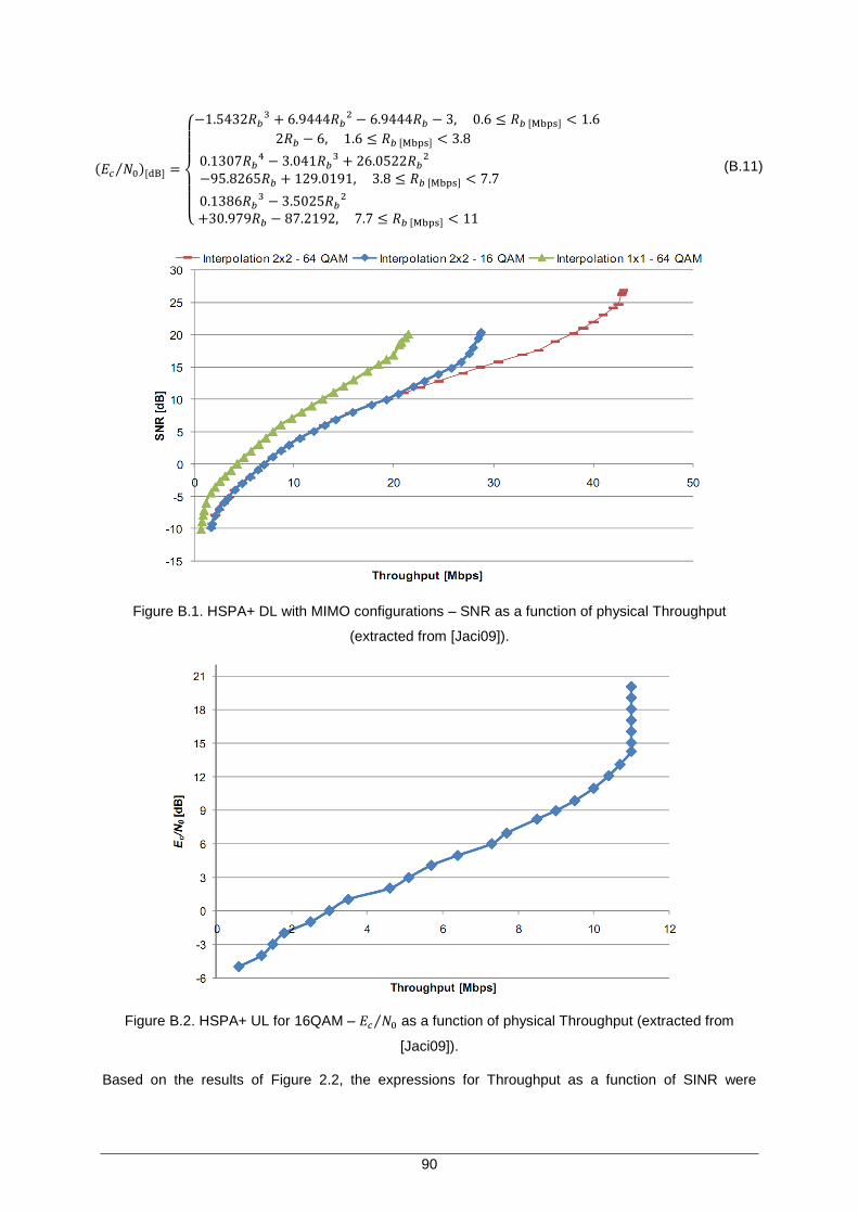
90
(B.11)
Figure B.1. HSPA+ DL with MIMO configurations – SNR as a function of physical Throughput
(extracted from [Jaci09]).
Figure B.2. HSPA+ UL for 16QAM – as a function of physical Throughput (extracted from
[Jaci09]).
Based on the results of Figure 2.2, the expressions for Throughput as a function of SINR were
91
obtained, for HSPA+ in DL direction. Expressions for QPSK modulation in DL were once more
extrapolated from the ones for 16QAM, and data rate for QPSK is simply considered to be half of the
one for 16QAM.
Considering a SISO configuration, with 16QAM, one has for DL:
(B.12)
For SISO configuration and 64QAM, the DL throughput is given by:
(B.13)
For SIMO 1 2 configuration, with 16QAM, the DL throughput is obtained using:
(B.14)
Considering a SIMO 1 2 configuration and 64QAM, throughput for DL is given by:
(B.15)
For MIMO 2 2 configuration, 16QAM, the DL throughput is:
(B.16)
For MIMO 2 2, with 64QAM, the DL throughput is computed using:
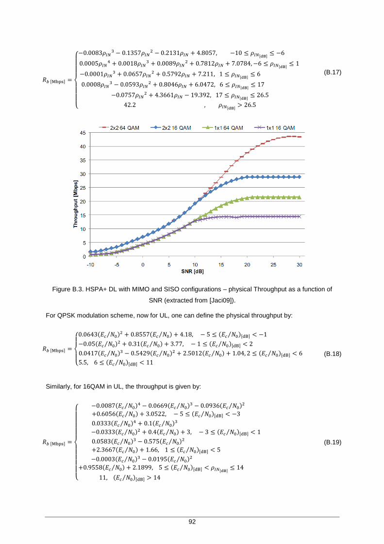
92
(B.17)
Figure B.3. HSPA+ DL with MIMO and SISO configurations – physical Throughput as a function of
SNR (extracted from [Jaci09]).
For QPSK modulation scheme, now for UL, one can define the physical throughput by:
(B.18)
Similarly, for 16QAM in UL, the throughput is given by:
(B.19)
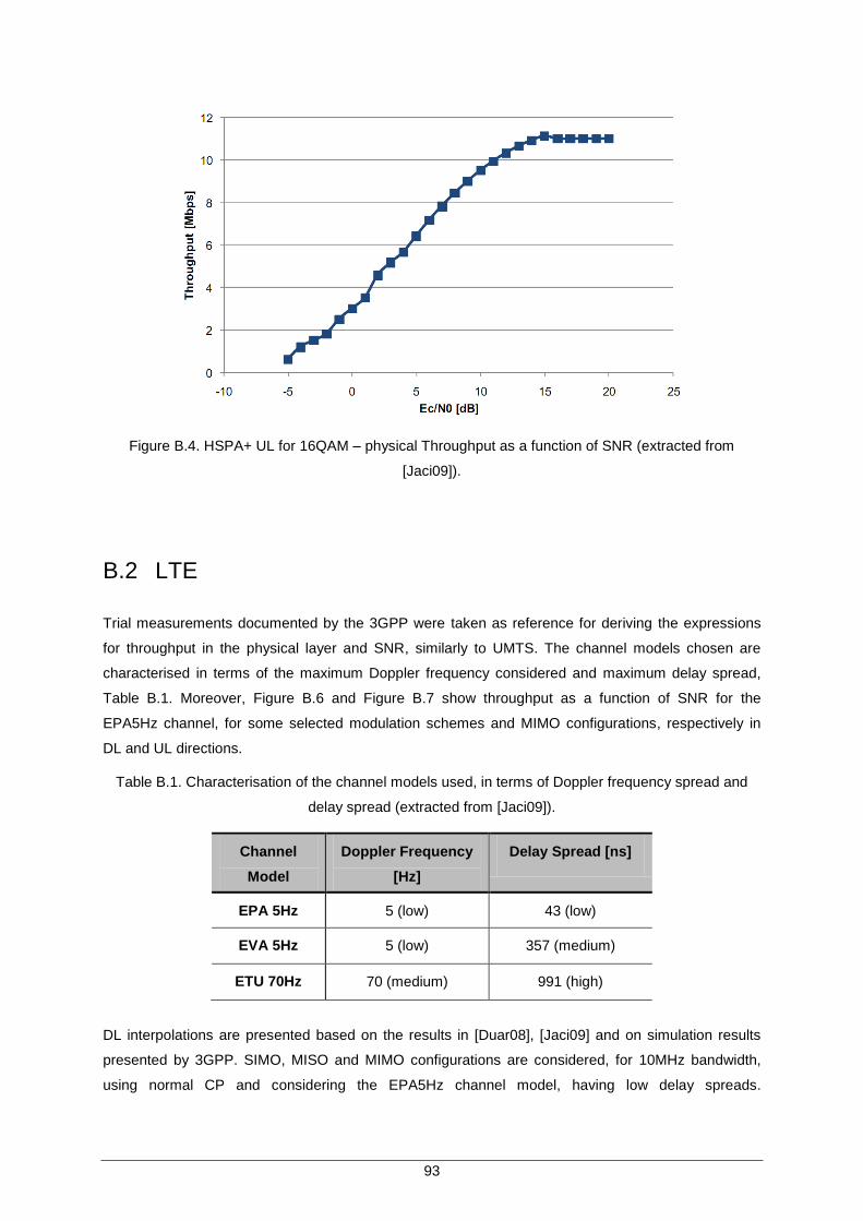
93
Figure B.4. HSPA+ UL for 16QAM – physical Throughput as a function of SNR (extracted from
[Jaci09]).
B.2 LTE
Trial measurements documented by the 3GPP were taken as reference for deriving the expressions
for throughput in the physical layer and SNR, similarly to UMTS. The channel models chosen are
characterised in terms of the maximum Doppler frequency considered and maximum delay spread,
Table B.1. Moreover, Figure B.6 and Figure B.7 show throughput as a function of SNR for the
EPA5Hz channel, for some selected modulation schemes and MIMO configurations, respectively in
DL and UL directions.
Table B.1. Characterisation of the channel models used, in terms of Doppler frequency spread and
delay spread (extracted from [Jaci09]).
Channel
Model
Doppler Frequency
[Hz]
Delay Spread [ns]
EPA 5Hz 5 (low) 43 (low)
EVA 5Hz 5 (low) 357 (medium)
ETU 70Hz 70 (medium) 991 (high)
DL interpolations are presented based on the results in [Duar08], [Jaci09] and on simulation results
presented by 3GPP. SIMO, MISO and MIMO configurations are considered, for 10MHz bandwidth,
using normal CP and considering the EPA5Hz channel model, having low delay spreads.
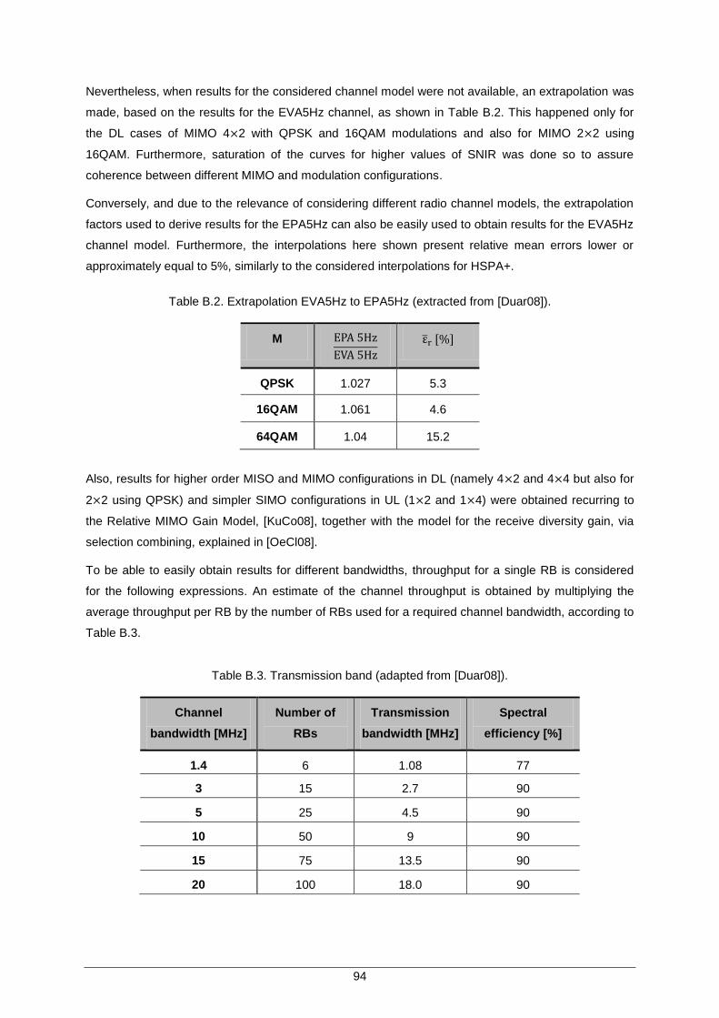
94
Nevertheless, when results for the considered channel model were not available, an extrapolation was
made, based on the results for the EVA5Hz channel, as shown in Table B.2. This happened only for
the DL cases of MIMO 4 2 with QPSK and 16QAM modulations and also for MIMO 2 2 using
16QAM. Furthermore, saturation of the curves for higher values of SNIR was done so to assure
coherence between different MIMO and modulation configurations.
Conversely, and due to the relevance of considering different radio channel models, the extrapolation
factors used to derive results for the EPA5Hz can also be easily used to obtain results for the EVA5Hz
channel model. Furthermore, the interpolations here shown present relative mean errors lower or
approximately equal to 5%, similarly to the considered interpolations for HSPA+.
Table B.2. Extrapolation EVA5Hz to EPA5Hz (extracted from [Duar08]).
M
QPSK 1.027 5.3
16QAM 1.061 4.6
64QAM 1.04 15.2
Also, results for higher order MISO and MIMO configurations in DL (namely 4 2 and 4 4 but also for
2 2 using QPSK) and simpler SIMO configurations in UL (1 2 and 1 4) were obtained recurring to
the Relative MIMO Gain Model, [KuCo08], together with the model for the receive diversity gain, via
selection combining, explained in [OeCl08].
To be able to easily obtain results for different bandwidths, throughput for a single RB is considered
for the following expressions. An estimate of the channel throughput is obtained by multiplying the
average throughput per RB by the number of RBs used for a required channel bandwidth, according to
Table B.3.
Table B.3. Transmission band (adapted from [Duar08]).
Channel
bandwidth [MHz]
Number of
RBs
Transmission
bandwidth [MHz]
Spectral
efficiency [%]
1.4 6 1.08 77
3 15 2.7 90
5 25 4.5 90
10 50 9 90
15 75 13.5 90
20 100 18.0 90
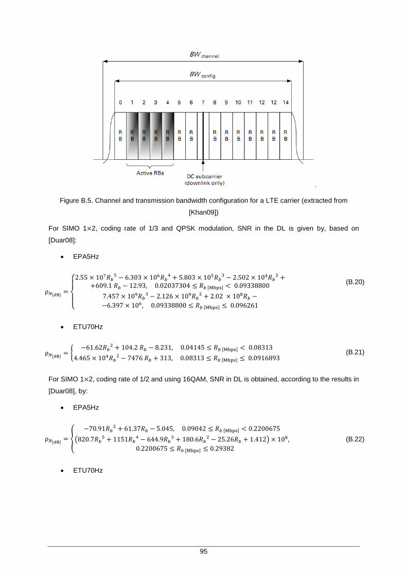
95
.
Figure B.5. Channel and transmission bandwidth configuration for a LTE carrier (extracted from
[Khan09])
For SIMO 1 2, coding rate of 1/3 and QPSK modulation, SNR in the DL is given by, based on
[Duar08]:
EPA5Hz
(B.20)
ETU70Hz
(B.21)
For SIMO 1 2, coding rate of 1/2 and using 16QAM, SNR in DL is obtained, according to the results in
[Duar08], by:
EPA5Hz
(B.22)
ETU70Hz
96
(B.23)
In SIMO 1 2, coding rate of 3/4 and 64QAM modulation, one gets for DL, [Duar08]:
EPA5Hz
(B.24)
ETU70Hz
(B.25)
For MIMO 2 2, coding rate of 1/2 and 16QAM, for DL, SNR is obtained based on the results in
[3GPP08a], [3GPP08b], [3GPP08c] and [3GPP08d]:
EPA5Hz
(B.26)
ETU70Hz
(B.27)
For MIMO 2 2, coding rate of 3/4 and 64QAM, based on the results in [3GPP08a], DL SNR is given
97
by:
EPA5Hz
(B.28)
ETU70Hz
(B.29)
In the case of the UL direction main results regarding MIMO 2 2 and 4 4 configurations in [Duar08]
were used, updated in some cases with the results documented by the 3GPP.
For MIMO 2 2, coding rate of 1/3 and QPSK, considering the UL direction, SNR is given by:
EPA5Hz
(B.30)
ETU70Hz
(B.31)
Similarly, for MIMO 2 2, coding rate of 3/4 and 16QAM, UL, SNR is given by:
EPA5Hz
(B.32)
ETU70Hz
(B.33)
98
For MIMO 2 2, coding rate of 5/6 and 64QAM, UL, SNR is given by:
EPA5Hz
(B.34)
ETU70Hz
(B.35)
For a MIMO 2 4 configuration, coding rate of 1/3 and QPSK, in UL, SNR is given by:
EPA5Hz
(B.36)
ETU70Hz
(B.37)
For MIMO 2 4, coding rate of 3/4 and 16QAM, UL, SNR is obtained by:
EPA5Hz
(B.38)
ETU70Hz
(B.39)
For the case of MIMO 2 4, coding rate of 5/6 and 64QAM, UL, SNR is given by:
EPA5Hz
(B.40)
ETU70Hz
99
(B.41)
Considering throughput in the physical layer as a function of the SNR in LTE, interpolated expressions
were obtained.
For SIMO 1 2, coding rate of 1/3 and using QPSK, DL throughput is given by, [Duar08] e [3GPP08a]:
EPA5Hz
(B.42)
ETU70Hz
(B.43)
For SIMO 1 2, coding rate of 1/2 and 16QAM, DL throughput is given by, [Duar08] and [3GPP07]:
EPA5Hz
(B.44)
ETU70Hz
(B.45)
For SIMO 1 2, coding rate of 3/4 and 64QAM, DL throughput is obtained by, [Duar08]:
EPA5Hz
100
(B.46)
ETU70Hz
(B.47)
For MIMO 2 2, coding rate of 1/2 and 16QAM, DL throughput is given based on the results in
[3GPP08a], [3GPP08b], [3GPP08c] and [3GPP08d]:
EPA5Hz
(B.48)
ETU70Hz
(B.49)
Considering MIMO 2 2, coding rate of 3/4 and 64QAM, based on the results in [3GPP08a],
throughput in the DL is given by:
EPA5Hz
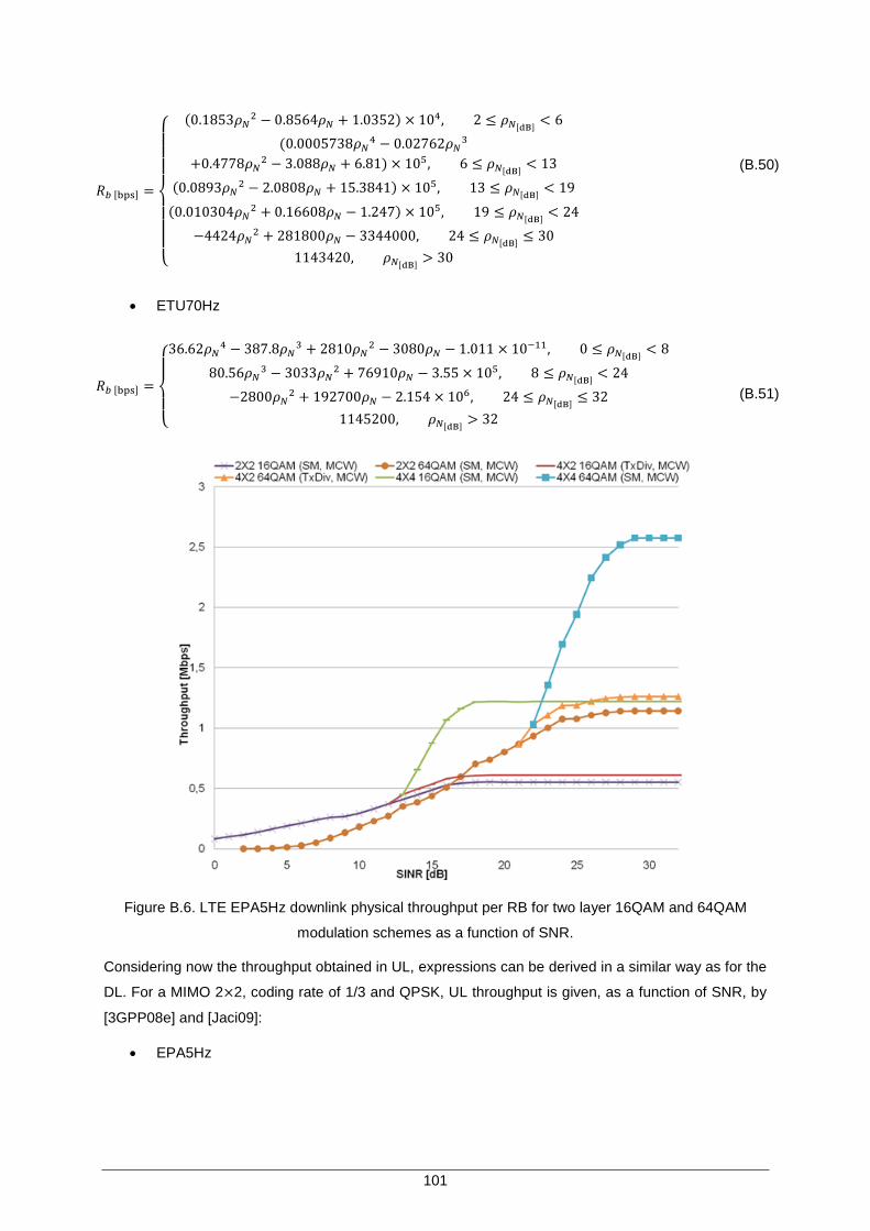
101
(B.50)
ETU70Hz
(B.51)
Figure B.6. LTE EPA5Hz downlink physical throughput per RB for two layer 16QAM and 64QAM
modulation schemes as a function of SNR.
Considering now the throughput obtained in UL, expressions can be derived in a similar way as for the
DL. For a MIMO 2 2, coding rate of 1/3 and QPSK, UL throughput is given, as a function of SNR, by
[3GPP08e] and [Jaci09]:
EPA5Hz
102
(B.52)
ETU70Hz
(B.53)
For MIMO 2 2, coding rate of 3/4 and 16QAM, UL throughput is given by [3GPP08e], [Duar08]:
EPA5Hz
(B.54)
ETU70Hz
(B.55)
For MIMO 2 2, coding rate of 5/6 and 64QAM, UL throughput is given by [3GPP08e] and [Jaci09]:
EPA5Hz
(B.56)
ETU70Hz
(B.57)
For MIMO 2 4, coding rate of 1/3 and QPSK, UL throughput is given by [Jaci09] and [3GPP08e]:
EPA5Hz
103
(B.58)
ETU70Hz
(B.59)
For MIMO 2 4, coding rate of 3/4 and 16QAM, UL throughput is computed as in [3GPP08e] and
[Jaci09]:
EPA5Hz
(B.60)
ETU70Hz
(B.61)
Considering a MIMO 2 4, coding rate of 5/6 and 64QAM, UL throughput is given based on the
measurements in [3GPP08e] and [Duar08]:
EPA5Hz
(B.62)
ETU70Hz
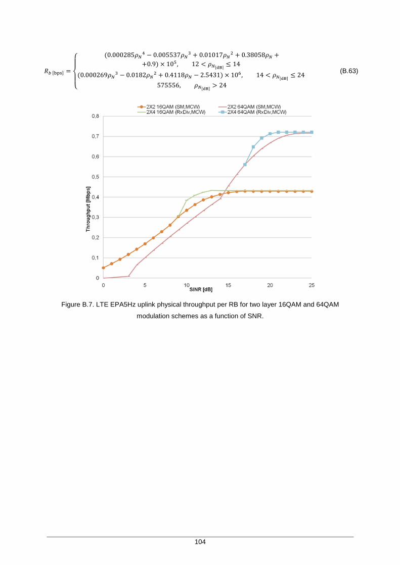
104
(B.63)
Figure B.7. LTE EPA5Hz uplink physical throughput per RB for two layer 16QAM and 64QAM
modulation schemes as a function of SNR.
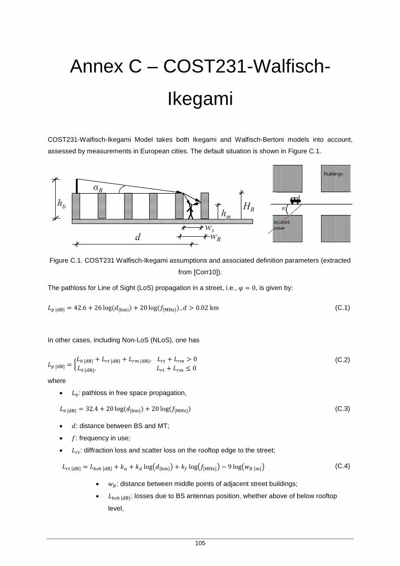
105
Annex C – COST231-Walfisch-
Ikegami Annex C – COST231-Walfisch-Ikegami
COST231-Walfisch-Ikegami Model takes both Ikegami and Walfisch-Bertoni models into account,
assessed by measurements in European cities. The default situation is shown in Figure C.1.
Figure C.1. COST231 Walfisch-Ikegami assumptions and associated definition parameters (extracted
from [Corr10]).
The pathloss for Line of Sight (LoS) propagation in a street, i.e., , is given by:
(C.1)
In other cases, including Non-LoS (NLoS), one has
(C.2)
where
: pathloss in free space propagation,
(C.3)
: distance between BS and MT;
: frequency in use;
: diffraction loss and scatter loss on the rooftop edge to the street;
(C.4)
: distance between middle points of adjacent street buildings;
: losses due to BS antennas position, whether above of below rooftop
level,
106
(C.5)
: BS height;
: building height.
: increase of the pathloss for BS antennas below the rooftops of the adjacent
buildings,
(C.6)
: dependence of multi-screen diffraction loss versus distance,
(C.7)
: dependence of multi-screen diffraction loss versus frequency,
(C.8)
: approximation for multiple screen diffraction loss,
(C.9)
: street width;
: MT height;
: street orientation loss,
(C.10)
: street orientation with respect to the direct radio link path.
The model is valid under the defined ranges for
f [800, 2000] MHz;
d [0.02, 5] km;
[4, 50] m;
[1, 3] m.
Although the frequency bands for HSPA+ DL are [2110,2170] MHz and for LTE are around 2500 MHz
and 2600 MHz, falling off the frequency range considered, this model is still the most adequate model
to consider in Urban and Suburban NLoS propagation environments.
The COST231-Walfisch-Ikegami Model standard deviation takes values from 4 dB to 7 dB, and the
107
error of the model increases as decreases relative to [Corr10]. In absence of specific values, the
following are recommended [Corr10]:
[20, 50] m;
;
;
;
.

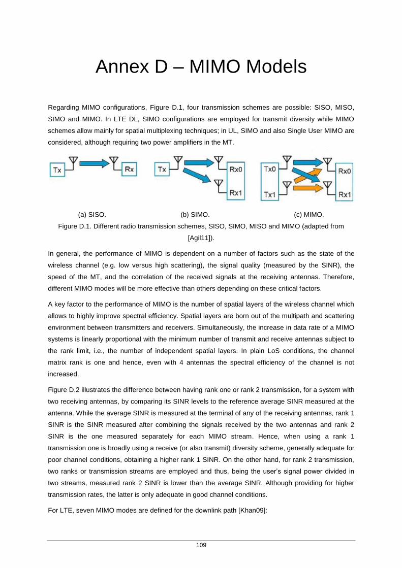
109
Annex D – MIMO Models Annex D – MIMO Models
Regarding MIMO configurations, Figure D.1, four transmission schemes are possible: SISO, MISO,
SIMO and MIMO. In LTE DL, SIMO configurations are employed for transmit diversity while MIMO
schemes allow mainly for spatial multiplexing techniques; in UL, SIMO and also Single User MIMO are
considered, although requiring two power amplifiers in the MT.
(a) SISO. (b) SIMO. (c) MIMO.
Figure D.1. Different radio transmission schemes, SISO, SIMO, MISO and MIMO (adapted from
[Agil11]).
In general, the performance of MIMO is dependent on a number of factors such as the state of the
wireless channel (e.g. low versus high scattering), the signal quality (measured by the SINR), the
speed of the MT, and the correlation of the received signals at the receiving antennas. Therefore,
different MIMO modes will be more effective than others depending on these critical factors.
A key factor to the performance of MIMO is the number of spatial layers of the wireless channel which
allows to highly improve spectral efficiency. Spatial layers are born out of the multipath and scattering
environment between transmitters and receivers. Simultaneously, the increase in data rate of a MIMO
systems is linearly proportional with the minimum number of transmit and receive antennas subject to
the rank limit, i.e., the number of independent spatial layers. In plain LoS conditions, the channel
matrix rank is one and hence, even with 4 antennas the spectral efficiency of the channel is not
increased.
Figure D.2 illustrates the difference between having rank one or rank 2 transmission, for a system with
two receiving antennas, by comparing its SINR levels to the reference average SINR measured at the
antenna. While the average SINR is measured at the terminal of any of the receiving antennas, rank 1
SINR is the SINR measured after combining the signals received by the two antennas and rank 2
SINR is the one measured separately for each MIMO stream. Hence, when using a rank 1
transmission one is broadly using a receive (or also transmit) diversity scheme, generally adequate for
poor channel conditions, obtaining a higher rank 1 SINR. On the other hand, for rank 2 transmission,
two ranks or transmission streams are employed and thus, being the user‟s signal power divided in
two streams, measured rank 2 SINR is lower than the average SINR. Although providing for higher
transmission rates, the latter is only adequate in good channel conditions.
For LTE, seven MIMO modes are defined for the downlink path [Khan09]:
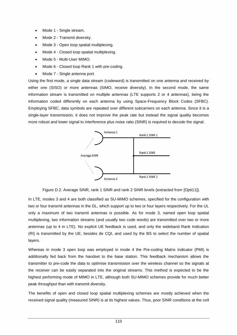
110
Mode 1 - Single stream.
Mode 2 - Transmit diversity.
Mode 3 - Open loop spatial multiplexing.
Mode 4 - Closed loop spatial multiplexing.
Mode 5 - Multi-User MIMO.
Mode 6 - Closed loop Rank 1 with pre-coding.
Mode 7 - Single antenna port.
Using the first mode, a single data stream (codeword) is transmitted on one antenna and received by
either one (SISO) or more antennas (SIMO, receive diversity). In the second mode, the same
information stream is transmitted on multiple antennas (LTE supports 2 or 4 antennas), being the
information coded differently on each antenna by using Space-Frequency Block Codes (SFBC).
Employing SFBC, data symbols are repeated over different subcarriers on each antenna. Since it is a
single-layer transmission, it does not improve the peak rate but instead the signal quality becomes
more robust and lower signal to interference plus noise ratio (SINR) is required to decode the signal.
Figure D.2. Average SINR, rank 1 SINR and rank 2 SINR levels (extracted from [Opti11]).
In LTE, modes 3 and 4 are both classified as SU-MIMO schemes, specified for the configuration with
two or four transmit antennas in the DL, which support up to two or four layers respectively. For the UL
only a maximum of two transmit antennas is possible. As for mode 3, named open loop spatial
multiplexing, two information streams (and usually two code words) are transmitted over two or more
antennas (up to 4 in LTE). No explicit UE feedback is used, and only the wideband Rank Indication
(RI) is transmitted by the UE, besides de CQI, and used by the BS to select the number of spatial
layers.
Whereas in mode 3 open loop was employed in mode 4 the Pre-coding Matrix Indicator (PMI) is
additionally fed back from the handset to the base station. This feedback mechanism allows the
transmitter to pre-code the data to optimise transmission over the wireless channel so the signals at
the receiver can be easily separated into the original streams. This method is expected to be the
highest performing mode of MIMO in LTE, although both SU-MIMO schemes provide for much better
peak throughput than with transmit diversity.
The benefits of open and closed loop spatial multiplexing schemes are mostly achieved when the
received signal quality (measured SINR) is at its highest values. Thus, poor SINR conditions at the cell
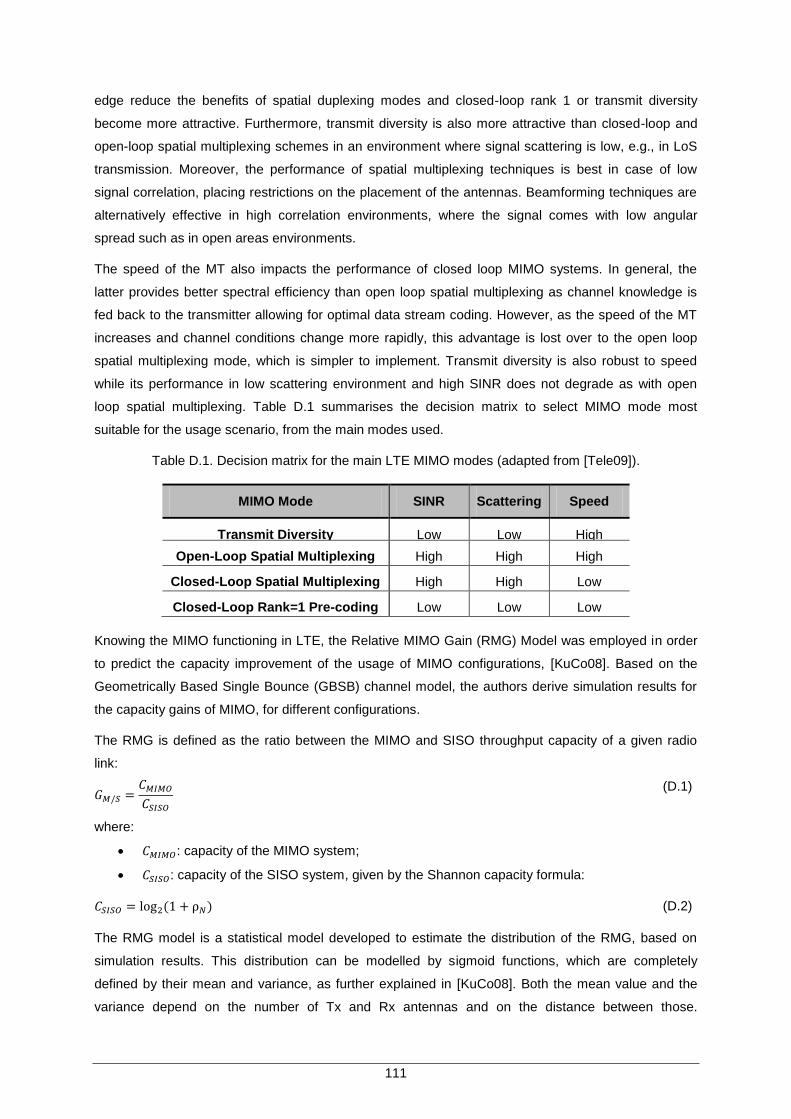
111
edge reduce the benefits of spatial duplexing modes and closed-loop rank 1 or transmit diversity
become more attractive. Furthermore, transmit diversity is also more attractive than closed-loop and
open-loop spatial multiplexing schemes in an environment where signal scattering is low, e.g., in LoS
transmission. Moreover, the performance of spatial multiplexing techniques is best in case of low
signal correlation, placing restrictions on the placement of the antennas. Beamforming techniques are
alternatively effective in high correlation environments, where the signal comes with low angular
spread such as in open areas environments.
The speed of the MT also impacts the performance of closed loop MIMO systems. In general, the
latter provides better spectral efficiency than open loop spatial multiplexing as channel knowledge is
fed back to the transmitter allowing for optimal data stream coding. However, as the speed of the MT
increases and channel conditions change more rapidly, this advantage is lost over to the open loop
spatial multiplexing mode, which is simpler to implement. Transmit diversity is also robust to speed
while its performance in low scattering environment and high SINR does not degrade as with open
loop spatial multiplexing. Table D.1 summarises the decision matrix to select MIMO mode most
suitable for the usage scenario, from the main modes used.
Table D.1. Decision matrix for the main LTE MIMO modes (adapted from [Tele09]).
MIMO Mode SINR Scattering Speed
Transmit Diversity Low Low High
Open-Loop Spatial Multiplexing High High High
Closed-Loop Spatial Multiplexing High High Low
Closed-Loop Rank=1 Pre-coding Low Low Low
Knowing the MIMO functioning in LTE, the Relative MIMO Gain (RMG) Model was employed in order
to predict the capacity improvement of the usage of MIMO configurations, [KuCo08]. Based on the
Geometrically Based Single Bounce (GBSB) channel model, the authors derive simulation results for
the capacity gains of MIMO, for different configurations.
The RMG is defined as the ratio between the MIMO and SISO throughput capacity of a given radio
link:
(D.1)
where:
: capacity of the MIMO system;
: capacity of the SISO system, given by the Shannon capacity formula:
(D.2)
The RMG model is a statistical model developed to estimate the distribution of the RMG, based on
simulation results. This distribution can be modelled by sigmoid functions, which are completely
defined by their mean and variance, as further explained in [KuCo08]. Both the mean value and the
variance depend on the number of Tx and Rx antennas and on the distance between those.
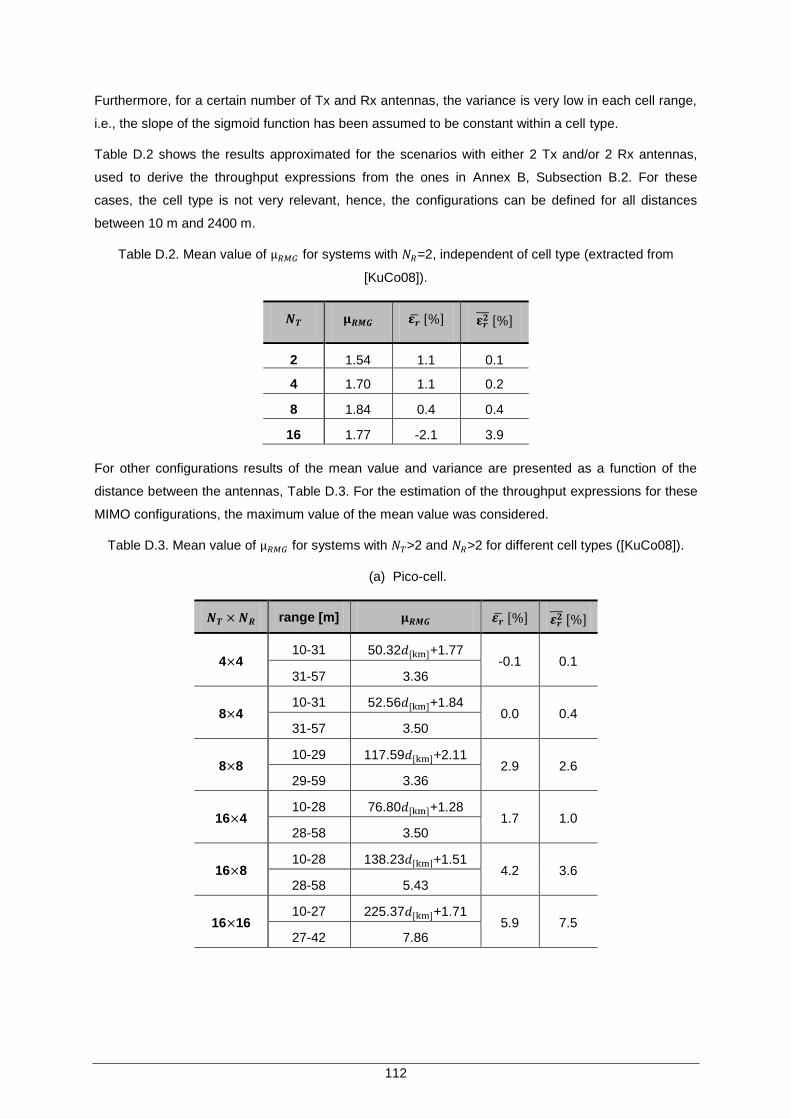
112
Furthermore, for a certain number of Tx and Rx antennas, the variance is very low in each cell range,
i.e., the slope of the sigmoid function has been assumed to be constant within a cell type.
Table D.2 shows the results approximated for the scenarios with either 2 Tx and/or 2 Rx antennas,
used to derive the throughput expressions from the ones in Annex B, Subsection B.2. For these
cases, the cell type is not very relevant, hence, the configurations can be defined for all distances
between 10 m and 2400 m.
Table D.2. Mean value of for systems with =2, independent of cell type (extracted from
[KuCo08]).
2 1.54 1.1 0.1
4 1.70 1.1 0.2
8 1.84 0.4 0.4
16 1.77 -2.1 3.9
For other configurations results of the mean value and variance are presented as a function of the
distance between the antennas, Table D.3. For the estimation of the throughput expressions for these
MIMO configurations, the maximum value of the mean value was considered.
Table D.3. Mean value of for systems with >2 and >2 for different cell types ([KuCo08]).
(a) Pico-cell.
range [m]
4 4 10-31 50.32 +1.77
-0.1
0.1 31-57 3.36
8 4 10-31 52.56 +1.84
0.0
0.4 31-57 3.50
8 8 10-29 117.59 +2.11
2.9
2.6 29-59 3.36
16 4 10-28 76.80 +1.28
1.7
1.0 28-58 3.50
16 8 10-28 138.23 +1.51
4.2
3.6 28-58 5.43
16 16 10-27 225.37 +1.71
5.9
7.5 27-42 7.86
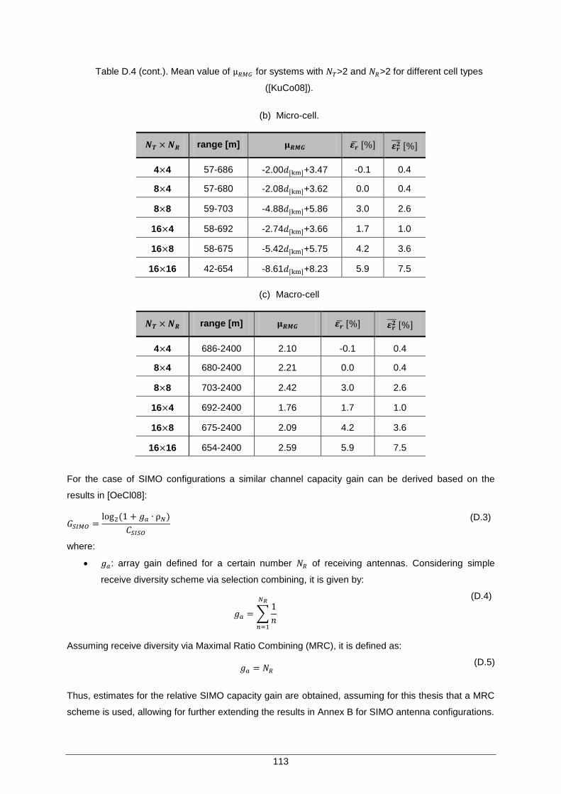
113
Table D.4 (cont.). Mean value of for systems with >2 and >2 for different cell types
([KuCo08]).
(b) Micro-cell.
range [m]
4 4 57-686 -2.00 +3.47 -0.1 0.4
8 4 57-680 -2.08 +3.62 0.0 0.4
8 8 59-703 -4.88 +5.86 3.0 2.6
16 4 58-692 -2.74 +3.66 1.7 1.0
16 8 58-675 -5.42 +5.75 4.2 3.6
16 16 42-654 -8.61 +8.23 5.9 7.5
(c) Macro-cell
range [m]
4 4 686-2400 2.10 -0.1 0.4
8 4 680-2400 2.21 0.0 0.4
8 8 703-2400 2.42 3.0 2.6
16 4 692-2400 1.76 1.7 1.0
16 8 675-2400 2.09 4.2 3.6
16 16 654-2400 2.59 5.9 7.5
For the case of SIMO configurations a similar channel capacity gain can be derived based on the
results in [OeCl08]:
(D.3) (
E.4)
where:
: array gain defined for a certain number of receiving antennas. Considering simple
receive diversity scheme via selection combining, it is given by:
(D.4) (D.5)
Assuming receive diversity via Maximal Ratio Combining (MRC), it is defined as:
(D.5) (
D.6)
Thus, estimates for the relative SIMO capacity gain are obtained, assuming for this thesis that a MRC
scheme is used, allowing for further extending the results in Annex B for SIMO antenna configurations.

114
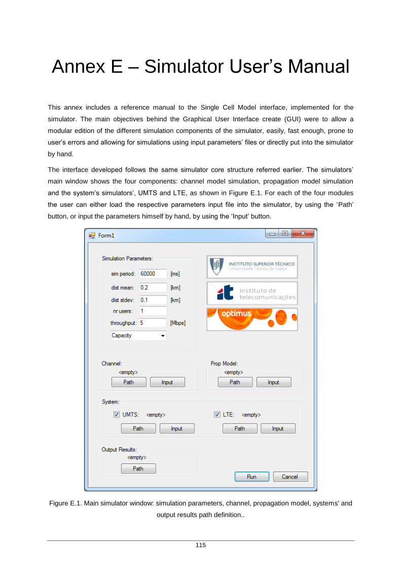
115
Annex E – Simulator User‟s Manual Annex E – Simulator User’s Manual
This annex includes a reference manual to the Single Cell Model interface, implemented for the
simulator. The main objectives behind the Graphical User Interface create (GUI) were to allow a
modular edition of the different simulation components of the simulator, easily, fast enough, prone to
user‟s errors and allowing for simulations using input parameters‟ files or directly put into the simulator
by hand.
The interface developed follows the same simulator core structure referred earlier. The simulators‟
main window shows the four components: channel model simulation, propagation model simulation
and the system‟s simulators‟, UMTS and LTE, as shown in Figure E.1. For each of the four modules
the user can either load the respective parameters input file into the simulator, by using the „Path‟
button, or input the parameters himself by hand, by using the „Input‟ button.
Figure E.1. Main simulator window: simulation parameters, channel, propagation model, systems' and
output results path definition..
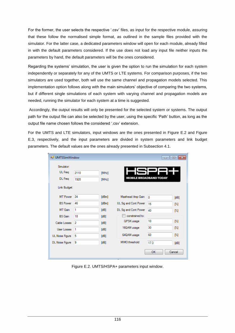
116
For the former, the user selects the respective „.csv‟ files, as input for the respective module, assuring
that these follow the normalised simple format, as outlined in the sample files provided with the
simulator. For the latter case, a dedicated parameters window will open for each module, already filled
in with the default parameters considered. If the use does not load any input file neither inputs the
parameters by hand, the default parameters will be the ones considered.
Regarding the systems‟ simulation, the user is given the option to run the simulation for each system
independently or separately for any of the UMTS or LTE systems. For comparison purposes, if the two
simulators are used together, both will use the same channel and propagation models selected. This
implementation option follows along with the main simulators‟ objective of comparing the two systems,
but if different single simulations of each system with varying channel and propagation models are
needed, running the simulator for each system at a time is suggested.
Accordingly, the output results will only be presented for the selected system or systems. The output
path for the output file can also be selected by the user, using the specific „Path‟ button, as long as the
output file name chosen follows the considered „.csv‟ extension.
For the UMTS and LTE simulators, input windows are the ones presented in Figure E.2 and Figure
E.3, respectively, and the input parameters are divided in system parameters and link budget
parameters. The default values are the ones already presented in Subsection 4.1.
Figure E.2. UMTS/HSPA+ parameters input window.
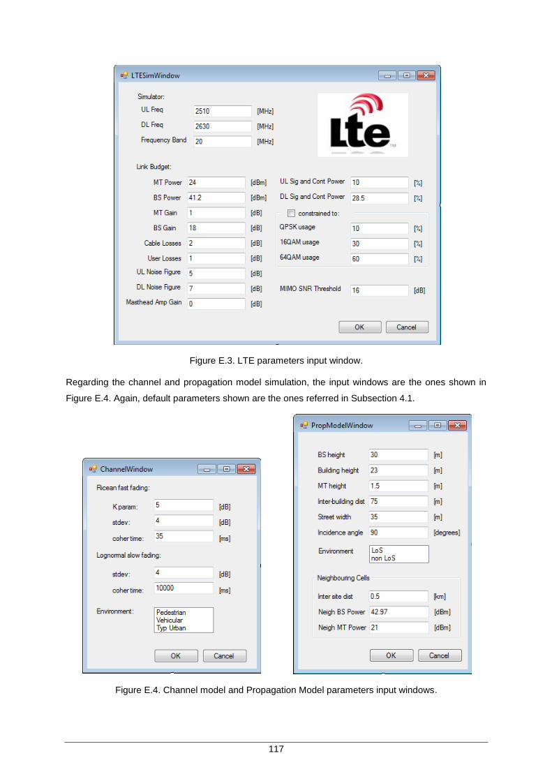
117
Figure E.3. LTE parameters input window.
Regarding the channel and propagation model simulation, the input windows are the ones shown in
Figure E.4. Again, default parameters shown are the ones referred in Subsection 4.1.
Figure E.4. Channel model and Propagation Model parameters input windows.

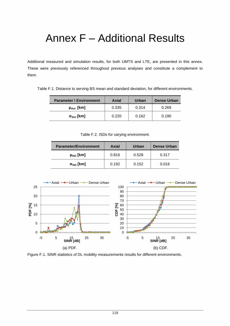
119
Annex F – Additional Results Annex F – Additional Results
Additional measured and simulation results, for both UMTS and LTE, are presented in this annex.
These were previously referenced throughout previous analyses and constitute a complement to
them.
Table F.1. Distance to serving BS mean and standard deviation, for different environments.
Parameter \ Environment Axial Urban Dense Urban
µdist [km] 0.335 0.314 0.269
σdist [km] 0.220 0.162 0.190
Table F.2. ISDs for varying environment.
Parameter/Environment Axial Urban Dense Urban
µISD [km] 0.816 0.528 0.317
σISD [km] 0.192 0.152 0.016
(a) PDF. (b) CDF.
Figure F.1. SINR statistics of DL mobility measurements results for different environments.
-5 5 15 25 35
0
5
10
15
20
25
SINR [dB]
PD
F [
%]
Axial Urban Dense Urban
-5 5 15 25 35
0
10
20
30
40
50
60
70
80
90
100
SINR [dB]
CD
F [
%]
Axial Urban Dense Urban
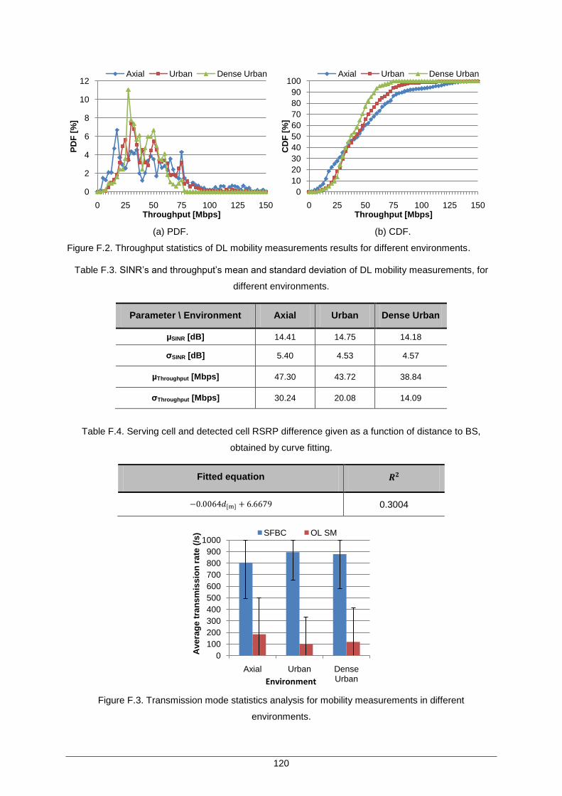
120
(a) PDF. (b) CDF.
Figure F.2. Throughput statistics of DL mobility measurements results for different environments.
Table F.3. SINR‟s and throughput‟s mean and standard deviation of DL mobility measurements, for
different environments.
Parameter \ Environment Axial Urban Dense Urban
µSINR [dB] 14.41 14.75 14.18
σSINR [dB] 5.40 4.53 4.57
µThroughput [Mbps] 47.30 43.72 38.84
σThroughput [Mbps] 30.24 20.08 14.09
Table F.4. Serving cell and detected cell RSRP difference given as a function of distance to BS,
obtained by curve fitting.
Fitted equation
0.3004
Figure F.3. Transmission mode statistics analysis for mobility measurements in different
environments.
0 25 50 75 100 125 150
0
2
4
6
8
10
12
Throughput [Mbps]
PD
F [
%]
Axial Urban Dense Urban
0 25 50 75 100 125 150
0
10
20
30
40
50
60
70
80
90
100
Throughput [Mbps]
CD
F [
%]
Axial Urban Dense Urban
0
100
200
300
400
500
600
700
800
900
1000
Axial Urban Dense Urban
Ave
rag
e t
ran
sm
iss
ion
rate
(/s
)
Environment
SFBC OL SM
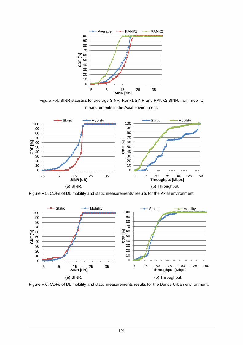
121
Figure F.4. SINR statistics for average SINR, Rank1 SINR and RANK2 SINR, from mobility
measurements in the Axial environment.
(a) SINR. (b) Throughput.
Figure F.5. CDFs of DL mobility and static measurements‟ results for the Axial environment.
(a) SINR. (b) Throughput.
Figure F.6. CDFs of DL mobility and static measurements results for the Dense Urban environment.
-5 5 15 25 35
0
10
20
30
40
50
60
70
80
90
100
SINR [dB]
CD
F [
%]
Average RANK1 RANK2
-5 5 15 25 35
0
10
20
30
40
50
60
70
80
90
100
SINR [dB]
CD
F [
%]
Static Mobility
0 25 50 75 100 125 150
0
10
20
30
40
50
60
70
80
90
100
Throughput [Mbps]
CD
F [
%]
Static Mobility
-5 5 15 25 35
0
10
20
30
40
50
60
70
80
90
100
SINR [dB]
CD
F [
%]
Static Mobility
0 25 50 75 100 125 150
0
10
20
30
40
50
60
70
80
90
100
Throughput [Mbps]
CD
F [
%]
Static Mobility
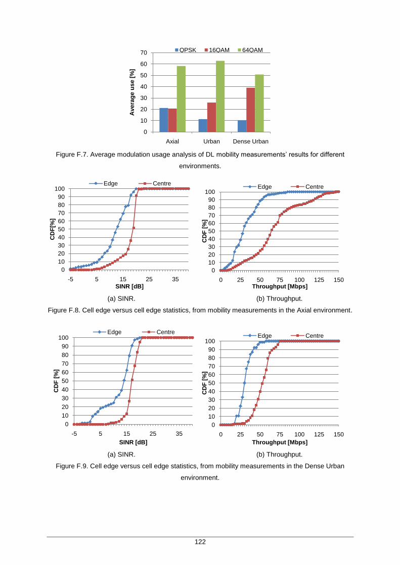
122
Figure F.7. Average modulation usage analysis of DL mobility measurements‟ results for different
environments.
(a) SINR. (b) Throughput.
Figure F.8. Cell edge versus cell edge statistics, from mobility measurements in the Axial environment.
(a) SINR. (b) Throughput.
Figure F.9. Cell edge versus cell edge statistics, from mobility measurements in the Dense Urban
environment.
0
10
20
30
40
50
60
70
Axial Urban Dense Urban
Ave
rag
e u
se
[%
]
QPSK 16QAM 64QAM
-5 5 15 25 35
0
10
20
30
40
50
60
70
80
90
100
SINR [dB]
CD
F[%
]
Edge Centre
0 25 50 75 100 125 150
0
10
20
30
40
50
60
70
80
90
100
Throughput [Mbps]
CD
F [
%]
Edge Centre
-5 5 15 25 35
0
10
20
30
40
50
60
70
80
90
100
SINR [dB]
CD
F [
%]
Edge Centre
0 25 50 75 100 125 150
0
10
20
30
40
50
60
70
80
90
100
Throughput [Mbps]
CD
F [
%]
Edge Centre
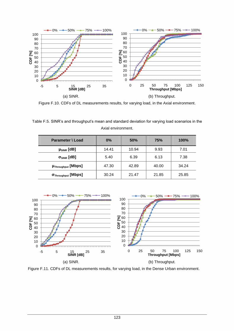
123
(a) SINR. (b) Throughput.
Figure F.10. CDFs of DL measurements results, for varying load, in the Axial environment.
Table F.5. SINR‟s and throughput‟s mean and standard deviation for varying load scenarios in the
Axial environment.
Parameter \ Load 0% 50% 75% 100%
µSINR [dB] 14.41 10.94 9.93 7.01
σSINR [dB] 5.40 6.39 6.13 7.38
µThroughput [Mbps] 47.30 42.89 40.00 34.24
σThroughput [Mbps] 30.24 21.47 21.85 25.85
(a) SINR. (b) Throughput.
Figure F.11. CDFs of DL measurements results, for varying load, in the Dense Urban environment.
-5 5 15 25 35
0
10
20
30
40
50
60
70
80
90
100
SINR [dB]
CD
F [
%]
0% 50% 75% 100%
0 25 50 75 100 125 150
0
10
20
30
40
50
60
70
80
90
100
Throughput [Mbps]
CD
F [
%]
0% 50% 75% 100%
-5 5 15 25 35
0
10
20
30
40
50
60
70
80
90
100
SINR [dB]
CD
F [
%]
0% 50% 75% 100%
0 25 50 75 100 125 150
0
10
20
30
40
50
60
70
80
90
100
Throughput [Mbps]
CD
F [
%]
0% 50% 75% 100%
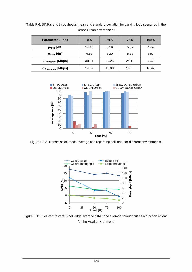
124
Table F.6. SINR‟s and throughput‟s mean and standard deviation for varying load scenarios in the
Dense Urban environment.
Parameter \ Load 0% 50% 75% 100%
µSINR [dB] 14.18 6.19 5.02 4.49
σSINR [dB] 4.57 5.20 5.72 5.67
µThroughput [Mbps] 38.84 27.25 24.15 23.69
σThroughput [Mbps] 14.09 13.98 14.55 16.92
Figure F.12. Transmission mode average use regarding cell load, for different environments.
Figure F.13. Cell centre versus cell edge average SINR and average throughput as a function of load,
for the Axial environment.
0
10
20
30
40
50
60
70
80
90
100
0 50 75 100
Ave
rag
e u
se
[%
]
Load [%]
SFBC Axial SFBC Urban SFBC Dense UrbanOL SM Axial OL SM Urban OL SM Dense Urban
0
20
40
60
80
100
120
140
-5
0
5
10
15
20
0 25 50 75 100
Thro
ugh
pu
t [M
bp
s]
SIN
R [
dB
]
Load [%]
Centre SINR Edge SINRCentre throughput Edge throughput
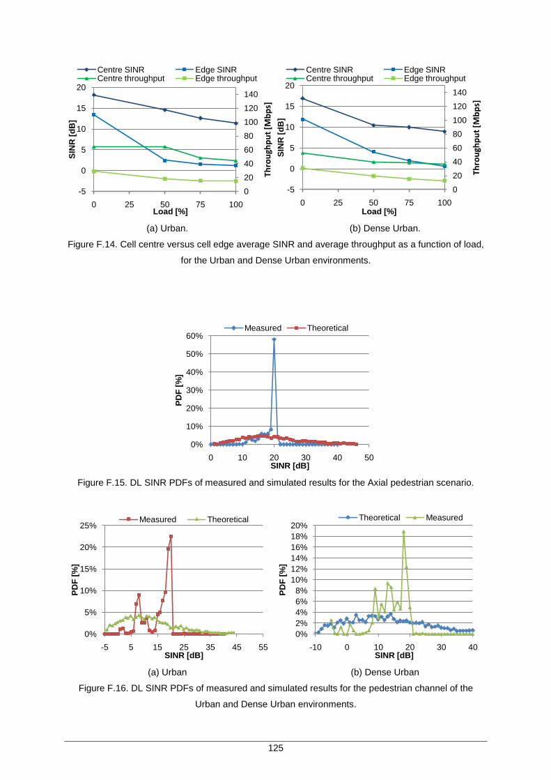
125
(a) Urban. (b) Dense Urban.
Figure F.14. Cell centre versus cell edge average SINR and average throughput as a function of load,
for the Urban and Dense Urban environments.
Figure F.15. DL SINR PDFs of measured and simulated results for the Axial pedestrian scenario.
(a) Urban (b) Dense Urban
Figure F.16. DL SINR PDFs of measured and simulated results for the pedestrian channel of the
Urban and Dense Urban environments.
0
20
40
60
80
100
120
140
-5
0
5
10
15
20
0 25 50 75 100
Thro
ugh
pu
t [M
bp
s]
SIN
R [
dB
]
Load [%]
Centre SINR Edge SINRCentre throughput Edge throughput
0
20
40
60
80
100
120
140
-5
0
5
10
15
20
0 25 50 75 100
Thro
ugh
pu
t [M
bp
s]
SIN
R [
dB
]
Load [%]
Centre SINR Edge SINRCentre throughput Edge throughput
0 10 20 30 40 50
0%
10%
20%
30%
40%
50%
60%
SINR [dB]
PD
F [
%]
Measured Theoretical
-5 5 15 25 35 45 55
0%
5%
10%
15%
20%
25%
SINR [dB]
PD
F [
%]
Measured Theoretical
-10 0 10 20 30 40
0%
2%
4%
6%
8%
10%
12%
14%
16%
18%
20%
SINR [dB]
PD
F [
%]
Theoretical Measured
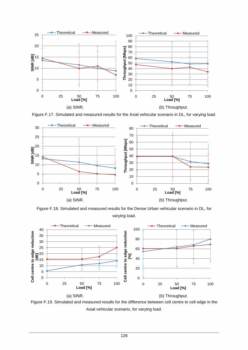
126
(a) SINR. (b) Throughput.
Figure F.17. Simulated and measured results for the Axial vehicular scenario in DL, for varying load.
(a) SINR. (b) Throughput.
Figure F.18. Simulated and measured results for the Dense Urban vehicular scenario in DL, for
varying load.
(a) SINR. (b) Throughput.
Figure F.19. Simulated and measured results for the difference between cell centre to cell edge in the
Axial vehicular scenario, for varying load.
0
5
10
15
20
25
0 25 50 75 100
SIN
R [
dB
]
Load [%]
Theoretical Measured
0
10
20
30
40
50
60
70
80
90
100
0 25 50 75 100
Th
rou
gh
pu
t [M
bp
s]
Load [%]
Theoretical Measured
0
5
10
15
20
25
30
0 25 50 75 100
SIN
R [
dB
]
Load [%]
Theoretical Measured
0
10
20
30
40
50
60
70
80
0 25 50 75 100
Th
rou
gh
pu
t [M
bp
s]
Load [%]
Theoretical Measured
0 25 50 75 100
0
5
10
15
20
25
30
35
40
Load [%]
Cell
ce
ntr
e t
o e
dg
e r
ed
uc
tio
n
[dB
]
Theoretical Measured
0 25 50 75 100
0
20
40
60
80
100
Load [%]
Cell
ce
ntr
e t
o e
dg
e r
ed
uc
tio
n
[%]
Theoretical Measured
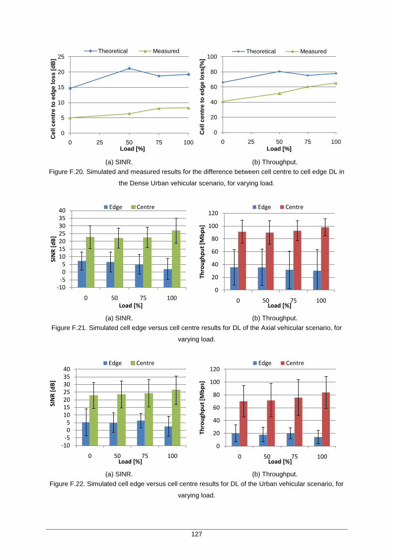
127
(a) SINR. (b) Throughput.
Figure F.20. Simulated and measured results for the difference between cell centre to cell edge DL in
the Dense Urban vehicular scenario, for varying load.
(a) SINR. (b) Throughput.
Figure F.21. Simulated cell edge versus cell centre results for DL of the Axial vehicular scenario, for
varying load.
(a) SINR. (b) Throughput.
Figure F.22. Simulated cell edge versus cell centre results for DL of the Urban vehicular scenario, for
varying load.
0 25 50 75 100
0
5
10
15
20
25
Load [%]
Ce
ll c
en
tre
to
ed
ge
lo
ss
[d
B]
Theoretical Measured
0 25 50 75 100
0
20
40
60
80
100
Load [%]
Ce
ll c
en
tre
to
ed
ge
lo
ss
[%]
Theoretical Measured
-10-505
10152025303540
0 50 75 100
SIN
R [
dB
]
Load [%]
Edge Centre
0
20
40
60
80
100
120
0 50 75 100
Thro
ugh
pu
t [M
bp
s]
Load [%]
Edge Centre
-10-505
10152025303540
0 50 75 100
SIN
R [
dB
]
Load [%]
Edge Centre
0
20
40
60
80
100
120
0 50 75 100
Thro
ugh
pu
t [M
bp
s]
Load [%]
Edge Centre
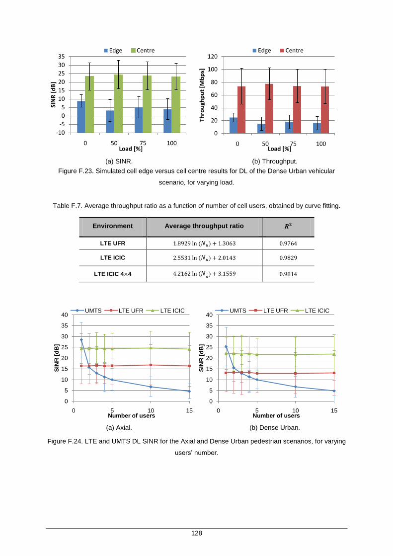
128
(a) SINR. (b) Throughput.
Figure F.23. Simulated cell edge versus cell centre results for DL of the Dense Urban vehicular
scenario, for varying load.
Table F.7. Average throughput ratio as a function of number of cell users, obtained by curve fitting.
Environment Average throughput ratio
LTE UFR
LTE ICIC
LTE ICIC 4 4
(a) Axial. (b) Dense Urban.
Figure F.24. LTE and UMTS DL SINR for the Axial and Dense Urban pedestrian scenarios, for varying
users‟ number.
-10
-5
0
5
10
15
20
25
30
35
0 50 75 100
SIN
R [
dB
]
Load [%]
Edge Centre
0
20
40
60
80
100
120
0 50 75 100
Thro
ugh
pu
t [M
bp
s]
Load [%]
Edge Centre
0
5
10
15
20
25
30
35
40
0 5 10 15
SIN
R [
dB
]
Number of users
UMTS LTE UFR LTE ICIC
0
5
10
15
20
25
30
35
40
0 5 10 15
SIN
R [
dB
]
Number of users
UMTS LTE UFR LTE ICIC
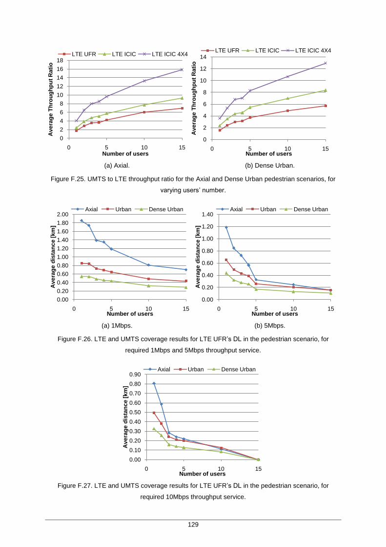
129
(a) Axial. (b) Dense Urban.
Figure F.25. UMTS to LTE throughput ratio for the Axial and Dense Urban pedestrian scenarios, for
varying users‟ number.
(a) 1Mbps. (b) 5Mbps.
Figure F.26. LTE and UMTS coverage results for LTE UFR‟s DL in the pedestrian scenario, for
required 1Mbps and 5Mbps throughput service.
Figure F.27. LTE and UMTS coverage results for LTE UFR‟s DL in the pedestrian scenario, for
required 10Mbps throughput service.
0
2
4
6
8
10
12
14
16
18
0 5 10 15
Ave
rag
e T
hro
ug
hp
ut
Ra
tio
Number of users
LTE UFR LTE ICIC LTE ICIC 4X4
0
2
4
6
8
10
12
14
0 5 10 15
Ave
rag
e T
hro
ug
hp
ut
Ra
tio
Number of users
LTE UFR LTE ICIC LTE ICIC 4X4
0.00
0.20
0.40
0.60
0.80
1.00
1.20
1.40
1.60
1.80
2.00
0 5 10 15
Ave
rag
e d
ista
nc
e [
km
]
Number of users
Axial Urban Dense Urban
0.00
0.20
0.40
0.60
0.80
1.00
1.20
1.40
0 5 10 15
Ave
rag
e d
ista
nc
e [
km
]
Number of users
Axial Urban Dense Urban
0.00
0.10
0.20
0.30
0.40
0.50
0.60
0.70
0.80
0.90
0 5 10 15
Ave
rag
e d
ista
nc
e [
km
]
Number of users
Axial Urban Dense Urban
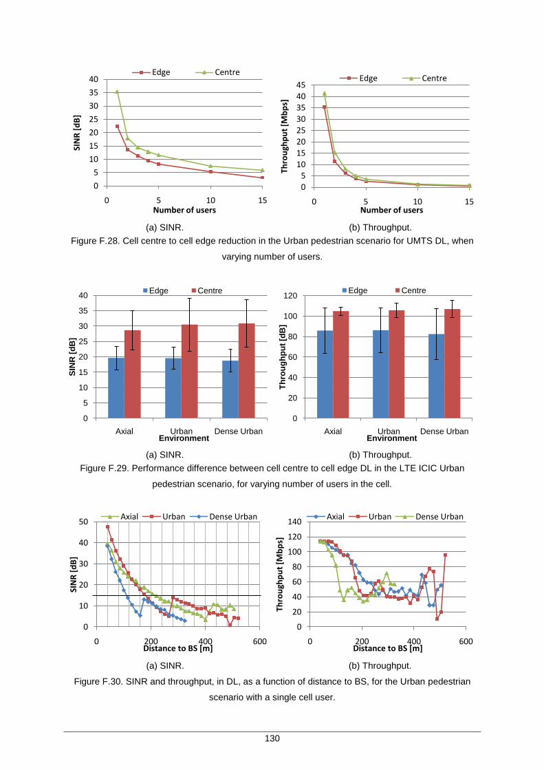
130
(a) SINR. (b) Throughput.
Figure F.28. Cell centre to cell edge reduction in the Urban pedestrian scenario for UMTS DL, when
varying number of users.
(a) SINR. (b) Throughput.
Figure F.29. Performance difference between cell centre to cell edge DL in the LTE ICIC Urban
pedestrian scenario, for varying number of users in the cell.
(a) SINR. (b) Throughput.
Figure F.30. SINR and throughput, in DL, as a function of distance to BS, for the Urban pedestrian
scenario with a single cell user.
0
5
10
15
20
25
30
35
40
0 5 10 15
SIN
R [
dB
]
Number of users
Edge Centre
05
1015202530354045
0 5 10 15
Thro
ugh
pu
t [M
bp
s]
Number of users
Edge Centre
0
5
10
15
20
25
30
35
40
Axial Urban Dense Urban
SIN
R [
dB
]
Environment
Edge Centre
0
20
40
60
80
100
120
Axial Urban Dense Urban
Th
rou
gh
pu
t [d
B]
Environment
Edge Centre
0
10
20
30
40
50
0 200 400 600
SIN
R [
dB
]
Distance to BS [m]
Axial Urban Dense Urban
0
20
40
60
80
100
120
140
0 200 400 600
Thro
ugh
pu
t [M
bp
s]
Distance to BS [m]
Axial Urban Dense Urban
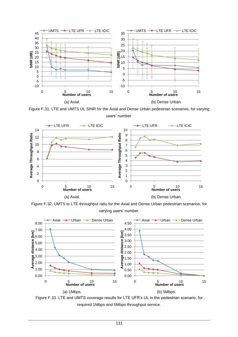
131
(a) Axial. (b) Dense Urban.
Figure F.31. LTE and UMTS UL SINR for the Axial and Dense Urban pedestrian scenarios, for varying
users‟ number.
(a) Axial. (b) Dense Urban.
Figure F.32. UMTS to LTE throughput ratio for the Axial and Dense Urban pedestrian scenarios, for
varying users‟ number.
(a) 1Mbps. (b) 5Mbps.
Figure F.33. LTE and UMTS coverage results for LTE UFR‟s UL in the pedestrian scenario, for
required 1Mbps and 5Mbps throughput service.
-10
-5
0
5
10
15
20
25
30
35
40
45
0 5 10 15
SIN
R [
dB
]
Number of users
UMTS LTE UFR LTE ICIC
-10
-5
0
5
10
15
20
25
30
35
0 5 10 15
SIN
R [
dB
]
Number of users
UMTS LTE UFR LTE ICIC
0
2
4
6
8
10
12
14
0 5 10 15
Ave
rag
e T
hro
ug
hp
ut
Rati
o
Number of users
LTE UFR LTE ICIC
0
1
2
3
4
5
6
7
8
9
10
0 5 10 15
Ave
rag
e T
hro
ug
hp
ut
Rati
o
Number of users
LTE UFR LTE ICIC
0.00
1.00
2.00
3.00
4.00
5.00
6.00
7.00
8.00
0 5 10 15
Ave
rag
e d
ista
nc
e [
km
]
Number of users
Axial Urban Dense Urban
0.00
0.50
1.00
1.50
2.00
2.50
3.00
3.50
4.00
4.50
0 5 10 15
Ave
rag
e d
ista
nc
e [
km
]
Number of users
Axial Urban Dense Urban
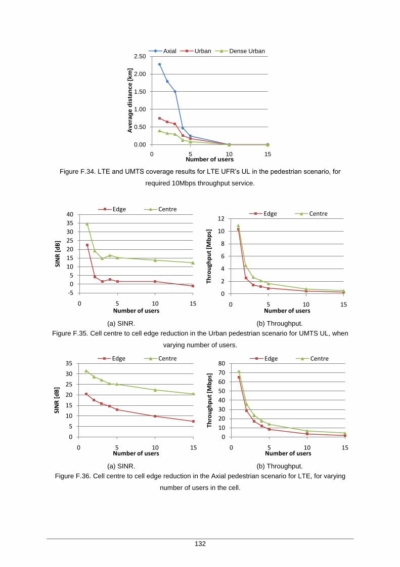
132
Figure F.34. LTE and UMTS coverage results for LTE UFR‟s UL in the pedestrian scenario, for
required 10Mbps throughput service.
(a) SINR. (b) Throughput.
Figure F.35. Cell centre to cell edge reduction in the Urban pedestrian scenario for UMTS UL, when
varying number of users.
(a) SINR. (b) Throughput.
Figure F.36. Cell centre to cell edge reduction in the Axial pedestrian scenario for LTE, for varying
number of users in the cell.
0.00
0.50
1.00
1.50
2.00
2.50
0 5 10 15
Ave
rag
e d
ista
nc
e [
km
]
Number of users
Axial Urban Dense Urban
-5
0
5
10
15
20
25
30
35
40
0 5 10 15
SIN
R [
dB
]
Number of users
Edge Centre
0
2
4
6
8
10
12
0 5 10 15
Thro
ugh
pu
t [M
bp
s]
Number of users
Edge Centre
0
5
10
15
20
25
30
35
0 5 10 15
SIN
R [
dB
]
Number of users
Edge Centre
0
10
20
30
40
50
60
70
80
0 5 10 15
Thro
ugh
pu
t [M
bp
s]
Number of users
Edge Centre
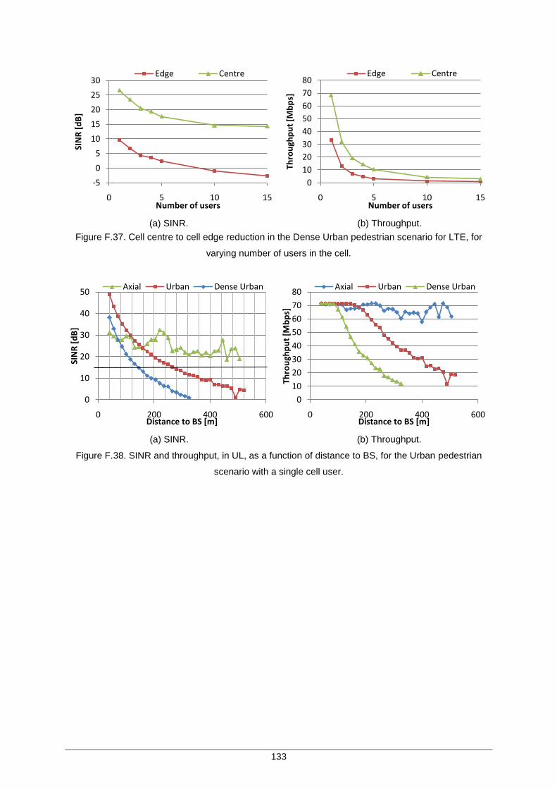
133
(a) SINR. (b) Throughput.
Figure F.37. Cell centre to cell edge reduction in the Dense Urban pedestrian scenario for LTE, for
varying number of users in the cell.
(a) SINR. (b) Throughput.
Figure F.38. SINR and throughput, in UL, as a function of distance to BS, for the Urban pedestrian
scenario with a single cell user.
-5
0
5
10
15
20
25
30
0 5 10 15
SIN
R [
dB
]
Number of users
Edge Centre
0
10
20
30
40
50
60
70
80
0 5 10 15
Thro
ugh
pu
t [M
bp
s]
Number of users
Edge Centre
0
10
20
30
40
50
0 200 400 600
SIN
R [
dB
]
Distance to BS [m]
Axial Urban Dense Urban
0
10
20
30
40
50
60
70
80
0 200 400 600
Thro
ugh
pu
t [M
bp
s]
Distance to BS [m]
Axial Urban Dense Urban

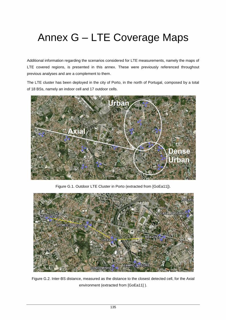
135
Annex G – LTE Coverage Maps Annex F – Additional Results
Additional information regarding the scenarios considered for LTE measurements, namely the maps of
LTE covered regions, is presented in this annex. These were previously referenced throughout
previous analyses and are a complement to them.
The LTE cluster has been deployed in the city of Porto, in the north of Portugal, composed by a total
of 18 BSs, namely an indoor cell and 17 outdoor cells.
Figure G.1. Outdoor LTE Cluster in Porto (extracted from [GoEa11]).
Figure G.2. Inter-BS distance, measured as the distance to the closest detected cell, for the Axial
environment (extracted from [GoEa11] ).
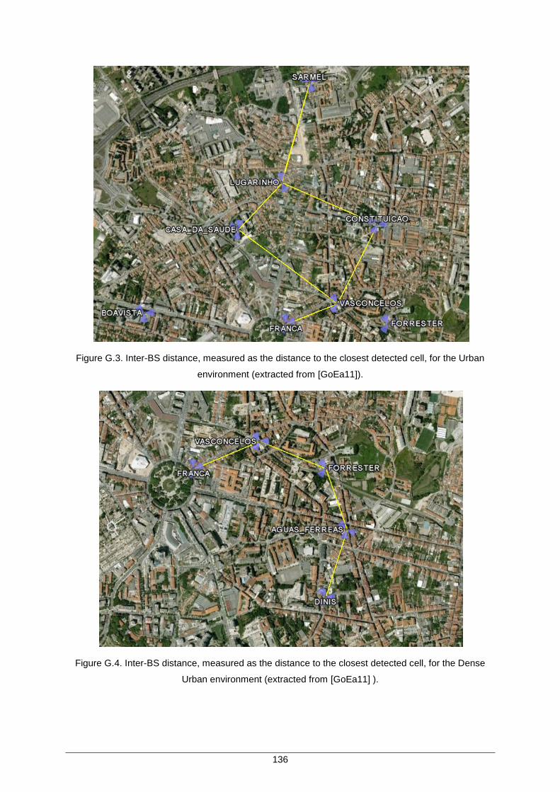
136
Figure G.3. Inter-BS distance, measured as the distance to the closest detected cell, for the Urban
environment (extracted from [GoEa11]).
Figure G.4. Inter-BS distance, measured as the distance to the closest detected cell, for the Dense
Urban environment (extracted from [GoEa11] ).
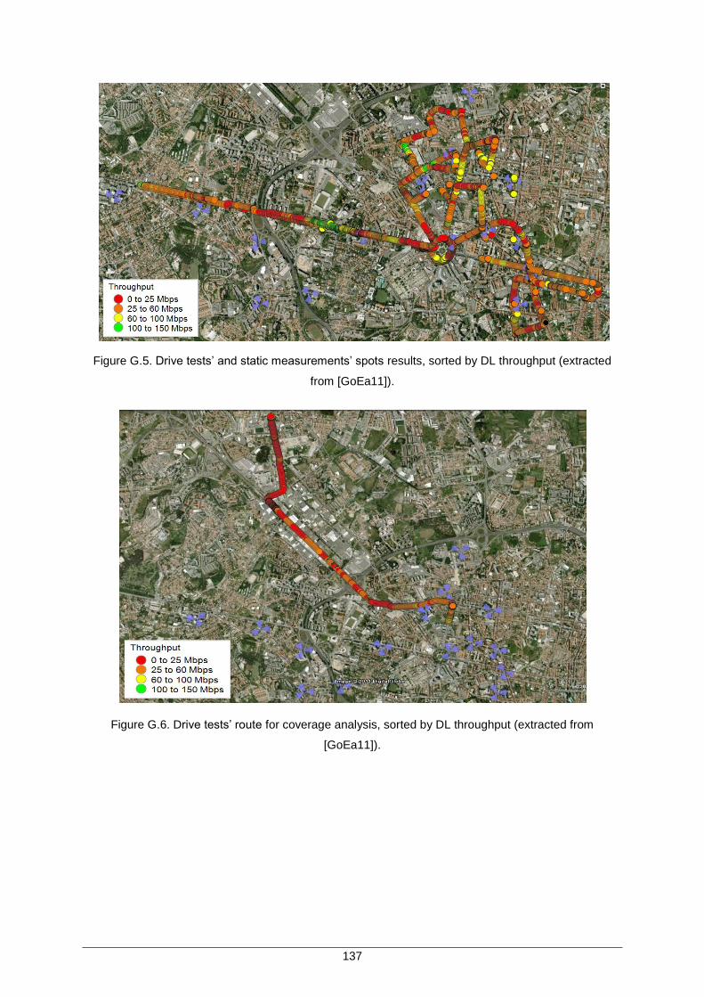
137
Figure G.5. Drive tests‟ and static measurements‟ spots results, sorted by DL throughput (extracted
from [GoEa11]).
Figure G.6. Drive tests‟ route for coverage analysis, sorted by DL throughput (extracted from
[GoEa11]).

139
Annex A – Link Budget
References
[3GPP07] 3GPP, Technical Specification Group - Radio Access Network Working, Collection of
PDSCH results, Report R4-072218, Jeju, Korea, Nov. 2007.
[3GPP08a] 3GPP, Technical Specification Group - Radio Access Network Working, PDSCH
Demodulation Ideal Results, Report R4-080194, Sorrento, Italy, Feb. 2008.
[3GPP08b] 3GPP, Technical Specification Group - Radio Access Network Working, PDSCH 2x2
MCW Ideal Simulation Results, Report R4-081792, Jeju, Korea, Aug. 2008.
[3GPP08c] 3GPP, Technical Specification Group - Radio Access Network Working, LTE UE PDSCH
demodulation results with impairments for MIMO-FDD case, Report R4-081439, Munich,
Germany, Jun. 2008.
[3GPP08d] 3GPP, Technical Specification Group - Radio Access Network Working, PDSCH MIMO
FDD results, Report R4-081129, Kansas City, USA, May 2008.
[3GPP08e] 3GPP, Technical Specification Group - Radio Access Network Working, PUSCH
Simulation Results, Report R4-071730, Shangai, China, Oct. 2007.
[3GPP09] 3GPP, Technical Specification Group Radio Access Network, Feasibility study for
evolved Universal Terrestrial Radio Access (UTRA) and Universal Terrestrial Radio
Access Network (UTRAN) (Release 9), Report TS 25.912, V9.0.0, Sep. 2009
(http://www.3gpp.org/ftp/specs/html-info/25912.htm).
[3GPP10a] 3GPP, Technical Specification Group Radio Access Network, BS Radio transmission and
Reception (FDD) (Release 99), Report TS 25.14.0, V9.6.0, Dec. 2010
(http://www.3gpp.org/ftp/Specs/html-info/25104.htm).
[3GPP10b] 3GPP, Technical Specification Group Radio Access Network, User Equipment (UE) radio
transmission and reception (FDD) (Release 9), Report TS 25.101, V9.6.0, Dec. 2010
(http://www.3gpp.org/ftp/specs/html-info/25101.htm).
[3GPP10c] 3GPP, Technical Specification Group Radio Access Network, Evolved Universal
Terrestrial Radio Access (E-UTRA) and Evolved Universal Terrestrial Radio Access
Network (E-UTRAN), Overall description, Stage 2 (Release 9), Report TS 36.300,
V.9.6.0, Dec. 2010 (http://www.3gpp.org/ftp/Specs/html-info/36300.htm).
[3GPP10d] 3GPP, Technical Specification Group Radio Access Network, Evolved Universal
140
Terrestrial Radio Access (E-UTRA); Base Station (BS) radio transmission and reception
(Release 9), Report TS 36.104, V.9.6.0, Dec. 2010
(http://www.3gpp.org/ftp/Specs/html-info/36104.htm).
[Agil07] Agilent, Agilent Technologies Solutions for 3GPP LTE, White Paper, USA, September
2007 (http://cp.literature.agilent.com/litweb/pdf/5989-6331EN.pdf).
[Agil11] Agilent, Transforming MIMO Test With Fast, Accurate Signal Creation and Channel
Emulation, Press Release, USA, Mar. 2011
(http://www.agilent.com/about/newsroom/tmnews/background/2008/01oct2008_pxb.html)
[ANAC11] ANACOM, Draft rules of the auction for allocation of rights for use of the frequency bands
of 450MHz, 900MHz, 1800MHz, 2.1GHz and 2.6 GHz, Public Consultation, Lisbon,
Portugal, 17th Mar. 2011
(http://www.anacom.pt/streaming/Regulation_auction_consultationDUF.pdf?contentId=10
93325&field=ATTACHED_FILE).
[Bati08] Batista,T.R., Capacity Increase in UMTS/HSPA+ Through the Use of MIMO Systems,
M.Sc. Thesis, Technical University of Lisbon, Lisbon, Portugal, 2008.
[Bati11] Batista,R.S., Performance Evaluation of UMTS/HSPA+ Data Transmission for Indoor
Coverage, M.Sc. Thesis, Technical University of Lisbon, Lisbon, Portugal, 2011.
[BEGG08] Bergman,J., Ericson,M., Gerstenberger,D., Göransson,B., Peisa,J. and Wager,S., “HSPA
Evolution – Boosting the performance of mobile broadband access”, Ericsson Review,
Vol.85, No.1, 2008.
[Carv09] Carvalho,G.N., Data Rate Performance Gains in UMTS Evolution at the Cellular Level,
M.Sc. Thesis, Technical University of Lisbon, Lisbon, Portugal, 2009.
[Cisc11] Cisco, Cisco Visual Networking Index: Global Mobile Data Traffic Forecast Update, 2010-
2015, White Paper, Cisco Systems, San Jose, California, USA, Feb. 2011
(http://www.cisco.com/en/US/solutions/collateral/ns341/ns525/ns537/ns705/ns827/white_
paper_c11-520862.pdf).
[Corr10] Correia,L.M., Mobile Communication Systems – Course Notes, IST-UTL, Lisbon,
Portugal, 2010.
[DEFJ06] Dahlman, E., Ekstrom, H., Furuskar, A., Jading, Y., Karlsson, J., Lundevall, M., Parkvall,
S., “3G Long-Term Evolution – Radio Interface Concepts and Performance Evaluation”,
in Proc. of VTC’06 Spring – 63rd
IEEE Vehicular Technology Conference, Melbourne,
Australia, May 2006.
[Duar08] Duarte, S., Analysis of Technologies for Long Term Evolution in UMTS, M.Sc. Thesis,
Technical University of Lisbon, Lisbon, Portugal, Sep.2008.
[Eric08] Ericsson, Initial field performance measurements of LTE, White Paper, Ericsson,
Stockholm, Sweden, Mar. 2008
141
(http://www.ericsson.com/res/thecompany/docs/publications/ericsson_review/2010/lte-
mimo.pdf).
[Eric10] Ericsson, Field trials of LTE with 4×4 MIMO, White Paper, Ericsson, Stockholm, Sweden,
Jan. 2010 (http://www.ericsson.com/res/thecompany/docs/publications
/ericsson_review/2010/lte-mimo.pdf).
[Eric11] Ericsson, Ericsson Achieves Three HSPA World Firsts, Press Release, Ericsson,
Stockholm, Sweden, Jan. 2011 (http://hugin.info/1061/R/1483840/419356.pdf).
[EsPe06] Esteves, H. and Pereira M., Impact of Intra- and Inter-Cellular Interference in UMTS
Capacity (in Portuguese), Dipl. Thesis, Technical University of Lisbon, Lisbon, Portugal,
June 2006.
[GGEM09] Greenstein, L.J., Ghassemzadeh, S.S., Erceg, V., Michelson, D.G., “Ricean K Factors in
Narrow-Band Fixed Wireless Channels: Theory, Experiments, and Statistical Models”,
IEEE Transactions on Vehicular Technology, Vol. 58, No. 8, Oct. 2009, pp. 4000-4012.
[GoEa11] http://earth.google.com/, May 2011.
[HoTo06] Holma, H. and Toskala, A., HSDPA/HSUPA for UMTS (1st Edition), John Wiley & Sons,
Chichester, UK, 2006.
[HoTo07] Holma, H. and Toskala, A., WCDMA for UMTS – HSPA Evolution and LTE (4th Edition),
John Wiley & Sons, Chichester, UK, 2007.
[HoTo09] Holma, H. and Toskala, A., LTE for UMTS – OFDMA and SC-FDMA Based Radio Access
(1st Edition), John Wiley & Sons, Chichester, UK, 2009.
[IkWR10] Ikuno, J.C., Wrulich, M., Rupp, M., “System Level Simulation of LTE Networks”, in Proc.
of VTC’10 Spring – 71st IEEE Vehicular Technology Conference, Taipei, Taiwan, June
2010.
[Jaci09] Jacinto, N.M., Performance Gains Evaluation from UMTS/HSPA+ to LTE at the Radio
Network Level, M.Sc. Thesis, Technical University of Lisbon, Lisbon, Portugal, 2009.
[JBGB09] Johansson, K., Bergman, J., Gerstenberger, D., Blomgren, M., Wallén, A., “Multi-Carrier
HSPA Evolution”, in Proc. of VTC’09 Spring – 69th IEEE Vehicular Technology
Conference, Barcelona, Spain, Apr. 2009.
[Khan09] Khan, F., LTE for 4G Mobile Broadband – Air Interface Technologies and Performance
(1st Edition), Cambridge University Press, Cambridge, UK, 2009.
[KuCo08] Kuipers, M., Correia, L.M., “Modelling the Relative MIMO Gain”, in Proc. of PIMRC’08 –
IEEE Personal, Indoor and Mobile Radio Communications, Cannes, France, Sep. 2008.
[LZZY07] Lei, H., Zhang, L., Zhang, X., Yang, D., “A Novel Multi-Cell OFDMA System Structure
using Fractional Frequency Reuse”, in Proc. of PIMRC’07 – IEEE Personal, Indoor and
Mobile Radio Communications, Athens, Greece, Sep. 2007.
142
[Mora10] Morais, M.C., Probability and Statistics – Course Notes (in Portuguese), Technical
University of Lisbon, Lisbon, Portugal, 2010 (http://www.math.ist.utl.pt/~mjmorais/2010-
09-12-NotasApoioPE-EdRevista-SeccaoFolhas.pdf).
[Moto07] Motorola, Long Term Evolution (LTE): Overview of LTE Air-Interface Technical White
Paper, White Paper, Motorola, USA, 2007
(http://business.motorola.com/experiencelte/pdf/LTEAirInterfaceWhitePaper.pdf).
[Moto09] Motorola, UMTS/HSPA to LTE Migration, White Paper, Motorola, USA, 2009
(http://www.motorola.com/web/Business/_Documents/static%20files/UMTS_to_LTE_Migr
ation_White_Paper.pdf).
[Moto10] Motorola, Motorola LTE Solution, LTE Systems Overview Brochure, Motorola, USA, 2010
(http://www.motorola.com/web/Business/Solutions/Industry%20Solutions/Service%20Pro
viders/Network%20Operators/LTE/_Document/LTE_Documents/Static_Files/LTE%20Sys
tems%20Overview%20Brochure.pdf).
[MWIB09] Mehlfuhrer, C., Wrulich, M., Ikuno, J.C., Bosanska, D., Rupp, M., “Simulating the Long
Term Evolution Physical Layer”, in Proc. of 17th European Signal Processing Conference,
Glasgow, UK, Aug. 2009.
[Neag11] http://www.gifted.uconn.edu/siegle/research/Correlation/alphaleve.htm, July, 2011.
[Noki09] Nokia Siemens Networks, LTE performance for initial deployments, White paper, Finland,
2009 (http://w3.nokiasiemensnetworks.com/NR/rdonlyres/46DBDFFE-0B36-40E8-8279-
5A56AADB8F6C/0/LTE_measurement_A4_1302.pdf).
[OeCl08] Oestges, C., Clerckx, B., MIMO Wireless Communications – From Real-World
Propagation to Space-Time Code Design (1st Edition), Elsevier, Oxford, UK, 2008.
[Open10] OPENET, Closing the Mobile Data Revenue Gap, White Paper, OPENET Telecom,
Dublin, Ireland, 2010 (http://ibmtelconewsletter.files.wordpress.com/2011/02/
wp_closing_mobile_data_revenue_gap_a4.pdf).
[Opti11] Private Communication, Optimus, 2011.
[Pede05] Pedersen, K.I., “Quality Based HSDPA Access Algorithms”, in Proc. of VTC’05 Fall – 62nd
IEEE Vehicular Technology Conference, Dallas, TX, USA, Sep. 2005.
[PeMo02] Pedersen, K.I., Mogensen, P.E., “The downlink orthogonality factors influence on
WCDMA system performance”, in Proc. of VTC’02 Fall – 56th IEEE Vehicular Technology
Conference, Vancouver, Canada, Dec. 2002.
[Pere11] Pereira, F., Audio and Video Communications – Course Notes, Technical University of
Lisbon, Lisbon, Portugal, 2011.
[Perg08] Perguiça, R., Comparison between UMTS/HSPA+ and WiMAX/IEEE 802.16e in Mobility
Scenarios, M.Sc. Thesis, Technical University of Lisbon, Lisbon, Portugal, Sep. 2008.
[PGBC10] Piro, G., Grieco, L.A., Boggia, G., Capozzi, F., Camarda, P., “Simulating LTE Cellular
143
Systems: an Open Source Framework”, IEEE Transactions on Vehicular Technology,
Vol. 60, No. 2, Feb. 2011, pp.498-513.
[PoMa09] Poikselkä, M. and Mayer, G., The IMS: IP Multimedia Concepts and Services (3rd
Edition), John Wiley & Sons, Chichester, UK, 2009.
[PoPo10] Porjazoski, M., Popovski, B., “Analysis of Intercell interference coordination by Fractional
frequency reuse in LTE”, in Proc. of SoftCOM 2010 International Conference on
Software, Telecommunications and Computer Networks (SoftCOM), Split, Croatia, Sep.
2010.
[PWST07] Peisa, J., Wager, S., Sågfors, M., Torsner, J., Göransson, B., Fulghum, T., Cozzo, C. and
Grant, S., “High Speed Packet Access Evolution – Concept and Technologies”, in Proc.
of VTC’07 - 65th
IEEE Vehicular Technology Conference, Dublin, Ireland, Apr. 2007.
[Rysa10] Rysavi, Transition to 4G – 3GPP Broadband Evolution to IMT-Advanced, Reserach
Report, Rysavi Research, Hood River, USA, Sep. 2010
(http://www.4gamericas.org/documents/3G_Americas_RysavyResearch_HSPA-
LTE_Advanced_FINALv1.pdf).
[SaNC10] Salo, J., Nur-Alam, M., Chang, K., Pratical Introduction to LTE Radio Planning, White
Paper, European Communications Engineering (ECE) Ltd, Espoo, Finland, Nov. 2010
(http://www.eceltd.com/lte_rf_wp_02Nov2010.pdf).
[Seid09] Seidel, E., Standardization updates on HSPA Evolution, Research Report, Nomor
Research GmbH, Munich, Germany, Mar. 2009
(http://www.3g4g.co.uk/Hspa/HSPAE_WP_0903_Nomor.pdf).
[SeTB09] Sesia, S., Toufik, I., Baker, M., LTE – The UMTS Long Term Evolution, From Theory to
Practice (1st Edition), John Wiley & Sons, Chichester, UK, 2009.
[Tele09] Telesystem Innovations, The Seven Modes of MIMO in LTE, White Paper, Telesystem
Innovations (TSI), Toronto, Canada, 2009 (http://www.slideshare.net/allabout4g/the-
seven-modes-of-mimo-in-ltepdf).
[VeCo11] Venes, J., Correia, L.M., “Performance of a Heterogeneous Network with UMTS, Wi-Fi
and WiMAX”, in Proc. of EUROCON – IEEE International Conference on Computer as a
Tool, Lisbon, Portugal, Apr. 2011.
[Voda10] Vodafone Portugal, Vodafone Portugal rolls out Mobile Broadband at speeds up to 43.2
Mbps, Press Release, Vodafone, Lisbon, Portugal, Oct. 2010
(http://www.vodafone.pt/main/A+Vodafone/EN/Press+Releases/pressreleases.htm?id=23
96&year=2010&quarter=4).
[XuMK08] Xuehong M., Maaref, A., Koon H. T., “Adaptive Soft Frequency Reuse for Inter-Cell
Interference Coordination in SC-FDMA Based 3GPP LTE Uplinks”, in Proc. of
GLOBECOM’08 – IEEE Global Communications Conference, New Orleans, L.A., USA,
Dec. 2008.
144
[Zeme08] Zemen, T., OFDMA/SC-FDMA Basics for 3GPP LTE (E-UTRA), Internal Report,
Forschungszentrum Telekommunikation Wien, Vienna, Austria, Apr. 2008
(http://www.nt.tuwien.ac.at/fileadmin/users/wkarner/OFDMA_SCFDMA.pdf).