Data Reconciliation in the process industries

Prof. Cesar de PradaDpt. Systems Engineering and

Automatic ControlUniversity of Valladolid, Spain

prada@autom.uva.es

Outline

PresentationMeasurements and informationData reconciliationGross errorsExamples:

– Sugar factory– Petrol refinery

Conclusions

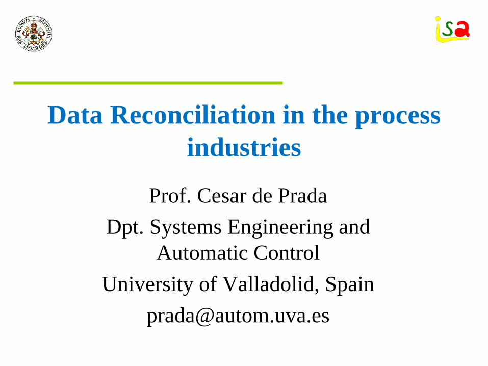
Today’s process plants

More instrumentationand systems

More technology More complex processes

More normsand regulations

Reducedtechnical staff

Higher marketpressures

More data than ever

From data to knowledge

Huge amount of data available in real time or historians.

Better instrumentation and new sensors

With less trained people in the control room or the technical teams, supporting tools are required for process safety, process behaviour predictions, help in Abnormal Situation Management,…

Models and simulations, decision support systems, etc., are recognized as elements to condense knowledge

The focus is on software applications at the MES level

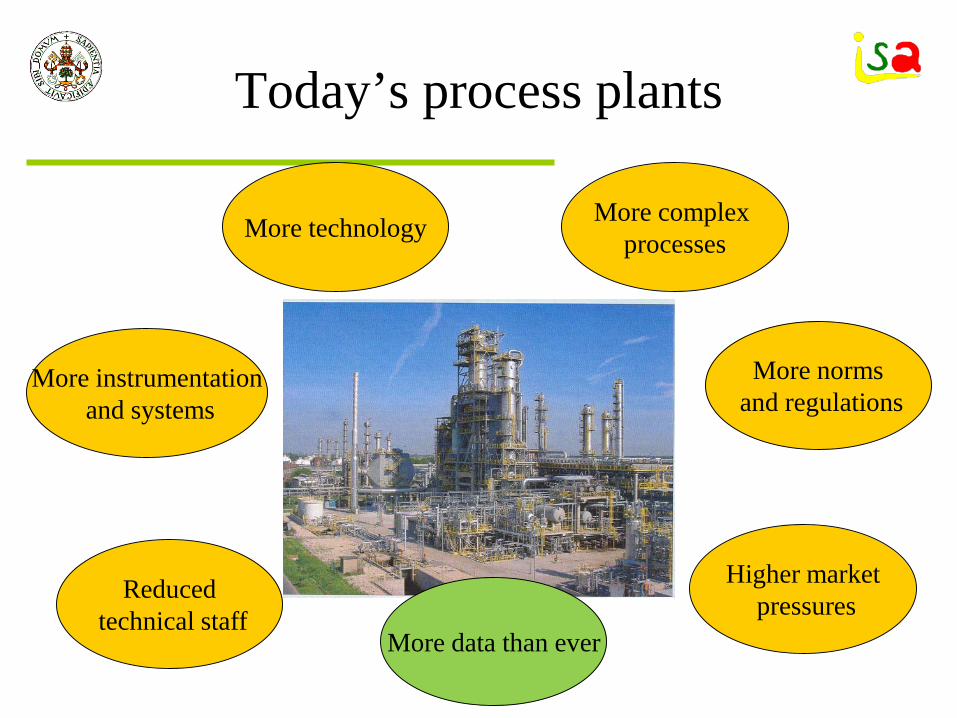
Models

There is a lot of interest in the optimal (economic) operation of the processes

Models play a key role in supporting the decision making process

Advanced Control and Economic Optimization are the right tools

Successful implementation requires suitable models and process information

Few tools for estimating earnings and improvements

Process

Basic Control

MPC

RTO

Dynamic

Static

SP

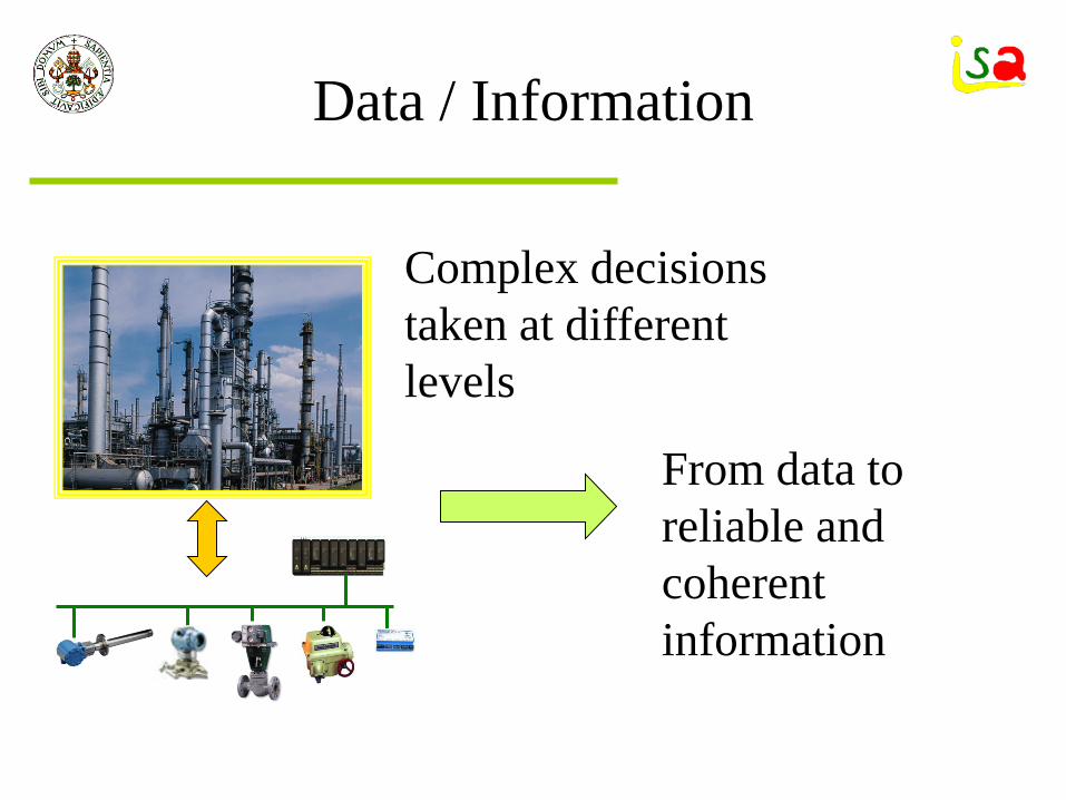
Data / Information

From data to reliable and coherent information

Complex decisions taken at different levels

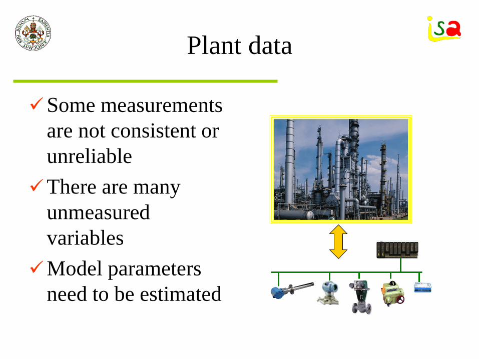
Plant data

Some measurements are not consistent or unreliable

There are many unmeasured variables

Model parameters need to be estimated

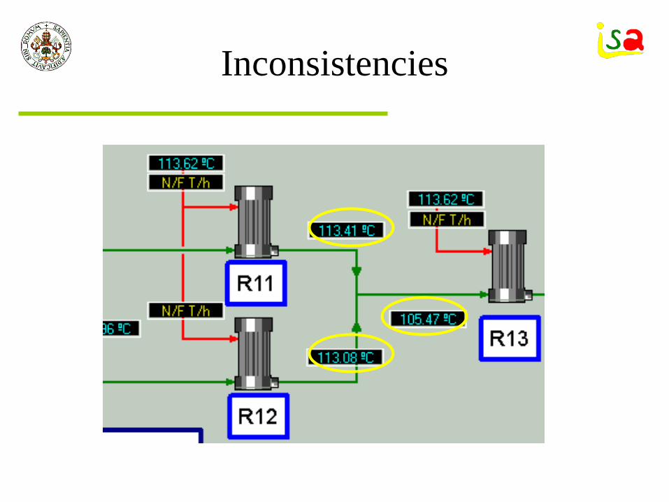
Inconsistencies

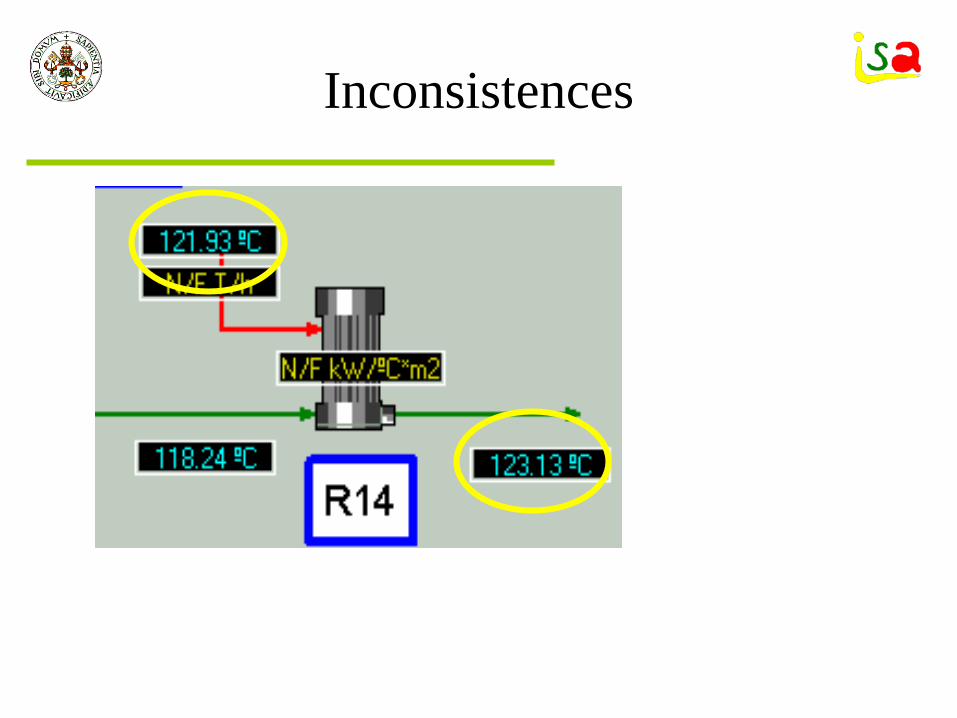
Inconsistences

Data reconciliation

Use plant/lab measurements and knowledge stored in the models to:– Estimate the values of all variables and model

parameters coherent with a process model and as close as possible to the measurements

– Detect and correct inconsistencies in the measurements

Formulated as an optimization problem

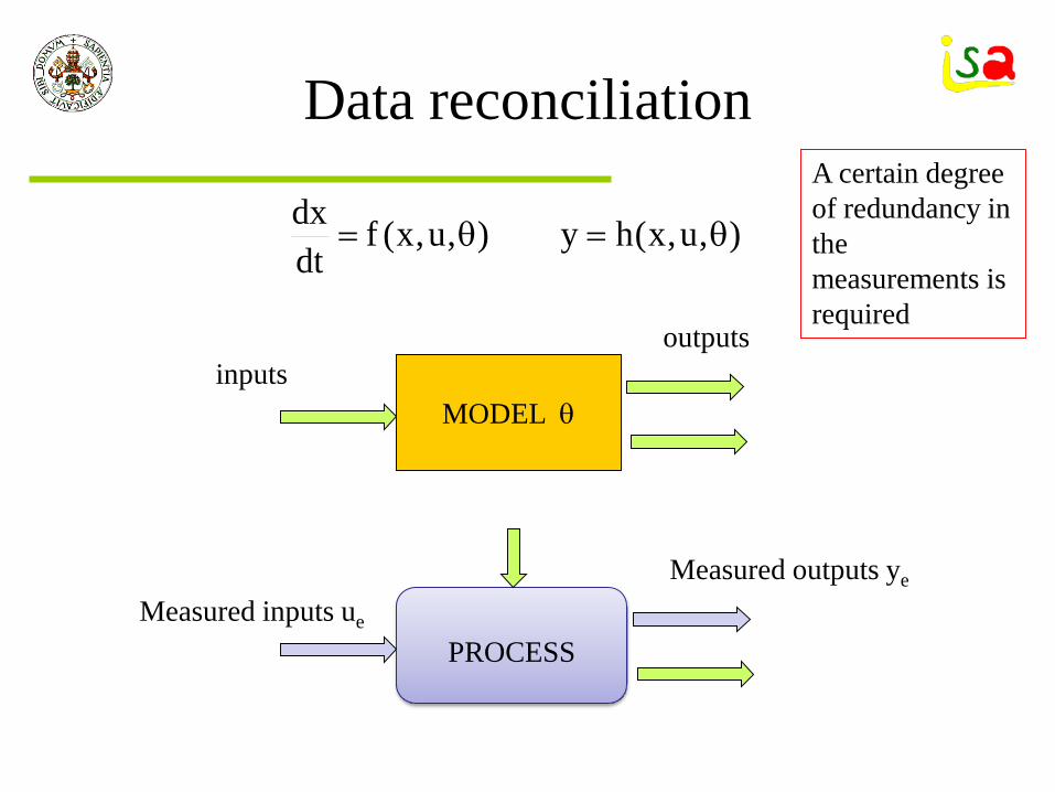
Data reconciliation

MODEL θinputs

PROCESS

outputs

Measured inputs ue

Measured outputs ye

),u,x(hy),u,x(fdtdx

θ=θ=

A certain degree of redundancy in the measurements is required

Redundancy

332211

321XFXFXF

FFF+=

+=

2 equations6 variables

More than 4 measurements are required to avoid having a unique or multiple solutions

Mass balances

F flowX composition

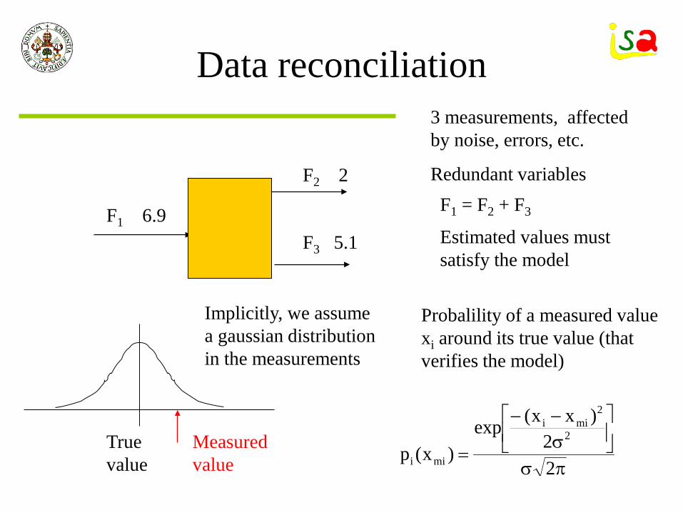
Data reconciliation

F1 6.9

F2 2

F3 5.1

3 measurements, affected by noise, errors, etc.

Redundant variablesF1 = F2 + F3

Estimated values must satisfy the model

True value

Measuredvalue

Probalility of a measured value xi around its true value (that verifies the model)

πσ

σ−−

=22

)xx(exp)x(p

2

2mii

mii

Implicitly, we assume a gaussian distribution in the measurements

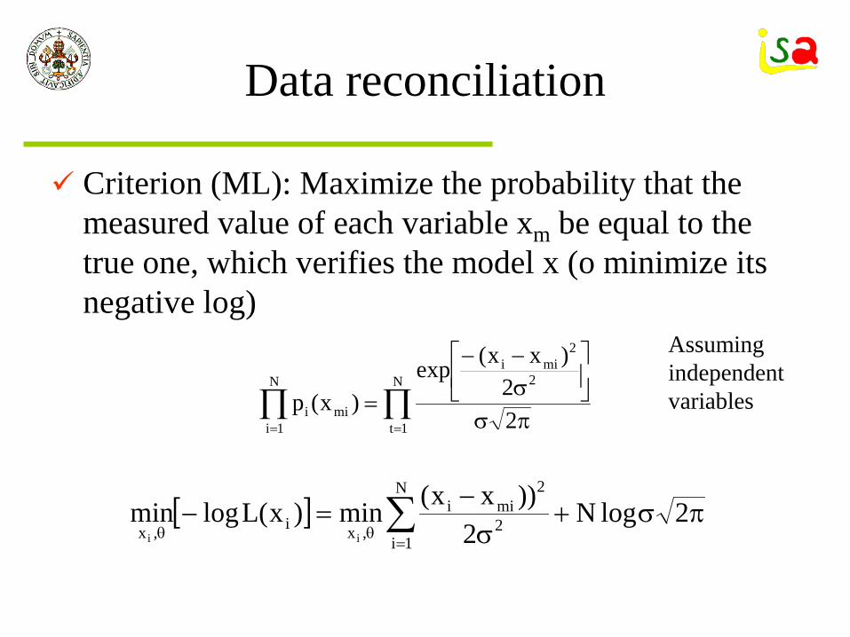
Data reconciliation

Criterion (ML): Maximize the probability that the measured value of each variable xm be equal to the true one, which verifies the model x (o minimize its negative log)

[ ] πσ+σ

−=− ∑

=θθ

2logN2

))xx(min)x(LlogminN

1i2

2mii

,xi,x ii

∏∏== πσ

σ−−

=N

1t

2

2mii

N

1imii 2

2)xx(exp

)x(p

Assuming independent variables

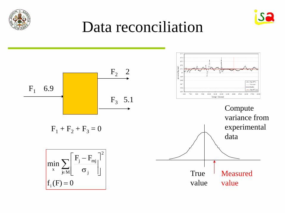
Data reconciliation

F1 6.9

F2 2

F3 5.1

F1 + F2 + F3 = 0

0)F(f

FFmin

i

Mj

2

j

mjj

x

=

σ−

∑∈ True

valueMeasuredvalue

Compute variance from experimental data

Data reconciliation

MODELOutputs y, u Measurements

ym, um

Optimizationproblem

Inputs u

θ

( ) ( )

0),u,y,x(g

),u,x(hy),u,x(fdtdx

uuyyαminmeasuredN

1i

2i,mii

2i,mii,u

≤θ

θ=θ=

−β+−∑=

θm measured values

Errors

Reconciled values

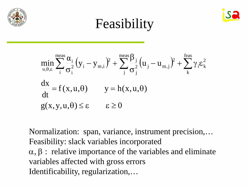
Feasibility

( ) ( )

0),u,y,x(g

),u,x(hy),u,x(fdtdx

uuyyαminfeas

k

2ki

meas

i

meas

j

2j,mj2

j

j2i,mi2

i

i,,u

≥εε≤θ

θ=θ=

εγ+−σβ

+−σ ∑∑ ∑εθ

Normalization: span, variance, instrument precision,…Feasibility: slack variables incorporatedα, β : relative importance of the variables and eliminate variables affected with gross errorsIdentificability, regularization,…

Gross errors

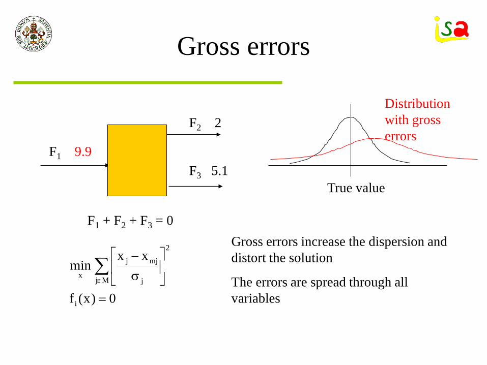
F1 9.9

F2 2

F3 5.1

F1 + F2 + F3 = 0

True value

Gross errors increase the dispersion and distort the solution

The errors are spread through all variables

Distribution with gross errors

0)x(f

xxmin

i

Mj

2

j

mjj

x

=

σ−

∑∈

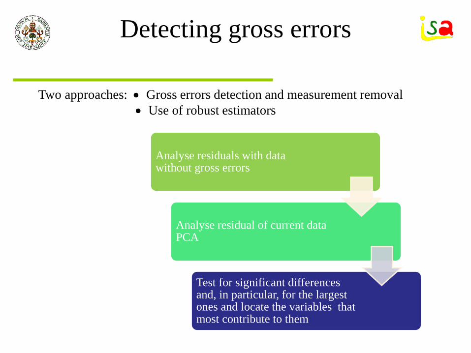
Detecting gross errors

Analyse residuals with data without gross errors

Analyse residual of current data PCA

Test for significant differences and, in particular, for the largest ones and locate the variables that most contribute to them

Two approaches: • Gross errors detection and measurement removal• Use of robust estimators

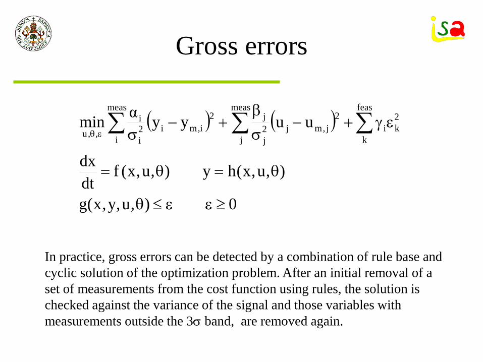
Gross errors

( ) ( )

0),u,y,x(g

),u,x(hy),u,x(fdtdx

uuyyαminfeas

k

2ki

meas

i

meas

j

2j,mj2

j

j2i,mi2

i

i,,u

≥εε≤θ

θ=θ=

εγ+−σβ

+−σ ∑∑ ∑εθ

In practice, gross errors can be detected by a combination of rule base and cyclic solution of the optimization problem. After an initial removal of a set of measurements from the cost function using rules, the solution is checked against the variance of the signal and those variables with measurements outside the 3σ band, are removed again.

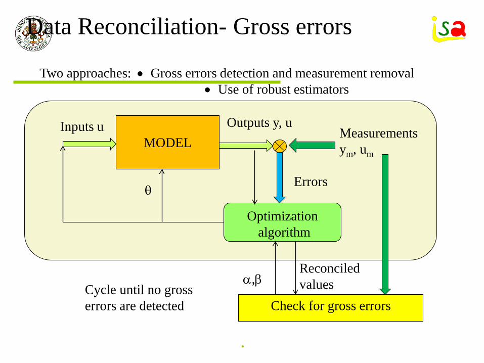
Data Reconciliation- Gross errors

Event • Place20/12/2019

MODELOutputs y, u

Measurements ym, um

Optimizationalgorithm

Inputs u

θ

Check for gross errors

α,βReconciled valuesCycle until no gross

errors are detected

Errors

Two approaches: • Gross errors detection and measurement removal• Use of robust estimators

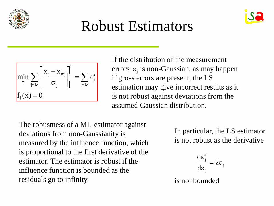
Robust Estimators

0)x(f

xxmin

i

Mj

2j

Mj

2

j

mjj

x

=

ε=

σ−

∑∑∈∈

If the distribution of the measurement errors εj is non-Gaussian, as may happen if gross errors are present, the LS estimation may give incorrect results as it is not robust against deviations from the assumed Gaussian distribution.

The robustness of a ML-estimator against deviations from non-Gaussianity is measured by the influence function, which is proportional to the first derivative of the estimator. The estimator is robust if the influence function is bounded as the residuals go to infinity.

In particular, the LS estimator is not robust as the derivative

jj

2j 2

dd

ε=εε

is not bounded

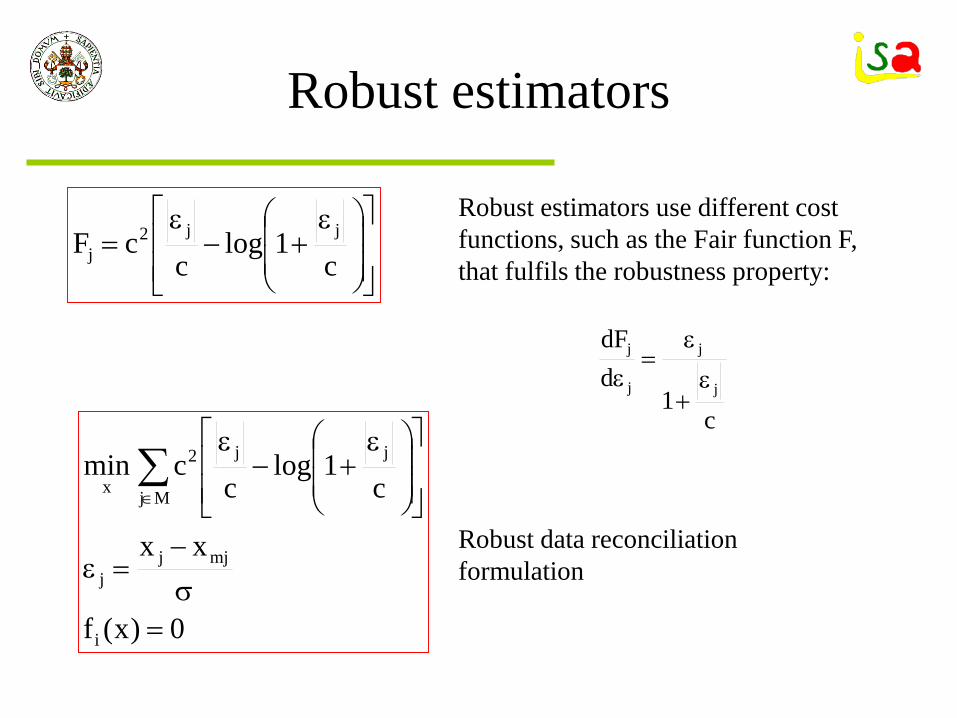
Robust estimators

0)x(f

xx

c1log

ccmin

i

mjjj

Mj

jj2

x

=σ−

=ε

ε+−

ε∑∈

Robust estimators use different cost functions, such as the Fair function F, that fulfils the robustness property:

ε+−

ε=

c1log

ccF jj2

j

c1

ddF

j

j

j

j

ε+

ε=

ε

Robust data reconciliation formulation

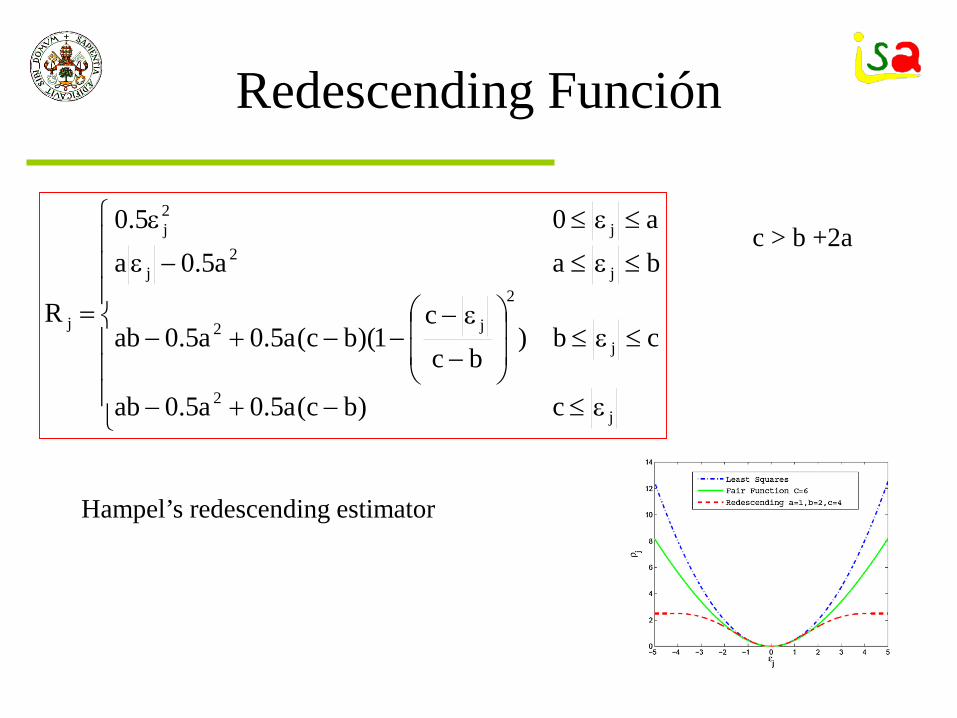
Redescending Función

ε≤−+−

≤ε≤

−

ε−−−+−

≤ε≤−ε

≤ε≤ε

=

j2

j

2

j2

j2

j

j2j

j

c)bc(a5.0a5.0ab

cb)bc

c1)(bc(a5.0a5.0ab

baa5.0aa05.0

R

Hampel’s redescending estimator

c > b +2a

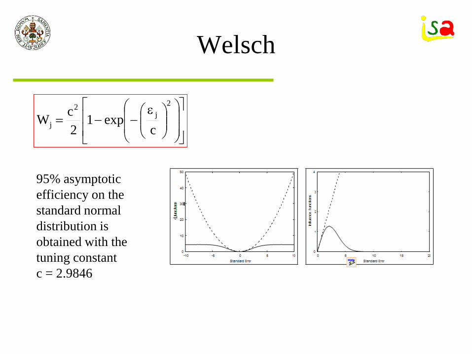
Welsch

ε−−=

2j

2

j cexp1

2cW

95% asymptotic efficiency on the standard normal distribution isobtained with the tuning constant c = 2.9846

Data reconciliation

Data reconciliation

Static Dynamic

Steady state detector

Data averaged over a period of time

Dynamic optimization problem

Batch

Open field

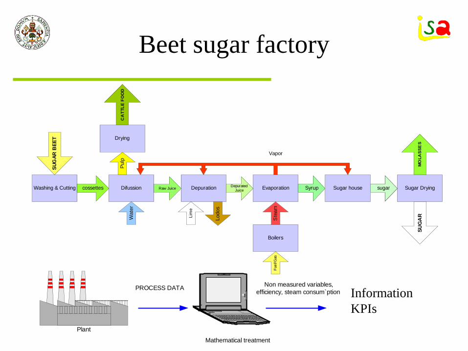
Beet sugar factory

Washing & Cutting

SUG

AR B

EET

Difussion Depuration Evaporation

Boilers

Sugar house Sugar Dryingcossettes Depurated Juice Syrup sugar

Ste

am

Drying

Pulp

SUG

ARWat

er

Fuel

/Gas

Lodo

s

Lim

eRaw Juice

CA

TTLE

FO

OD

MO

LASS

ES

Vapor

PROCESS DATA Non measured variables,

efficiency, steam consum`ption

Plant

Mathematical treatment

InformationKPIs

Sugar plant DR software

Main elements: Periodic characterization of the plant status, using a steady

model of the sugar plant. On line connection with the plan Distributed Control System

(DCS) to obtain, the measured variables necessary for the balances and model identification.

Data reconciliation, correcting measured variables in a way that the model is adjusted and calculating at the same time that unknown variables and model parameters.

As a by-product of the data reconciliation, key performance indicators are estimated from calculated values in the reconciliation.

Models

StaticMass energy balancesFlows, pressuresEquations and properties of the application

domainFormulated in the EcosimPro environmentMeasurements averaged for a period of timeRules to eliminate bad measurements

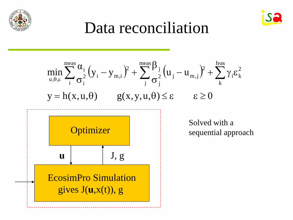
Data reconciliation

EcosimPro Simulationgives J(u,x(t)), g

Optimizer

u J, g

( ) ( )

0),u,y,x(g),u,x(hy

uuyyαminfeas

k

2ki

meas

i

meas

j

2j,mj2

j

j2i,mi2

i

i,,u

≥εε≤θθ=

εγ+−σβ

+−σ ∑∑ ∑εθ

Solved with a sequential approach

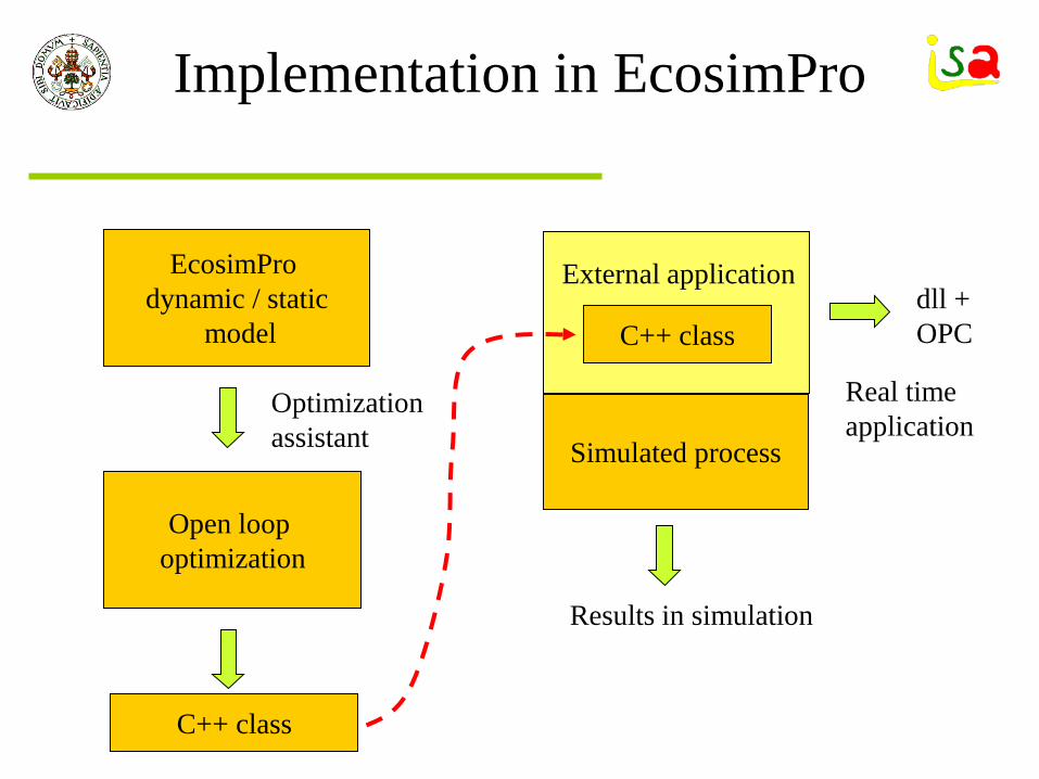
Implementation in EcosimPro

EcosimPro dynamic / static

model

Open loop optimization

Optimization assistant

C++ class

Simulated process

dll + OPC

Real time application

Results in simulation

C++ class

External application

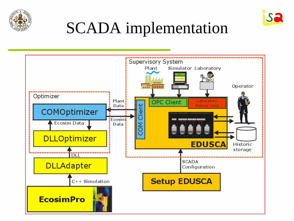
SCADA implementation

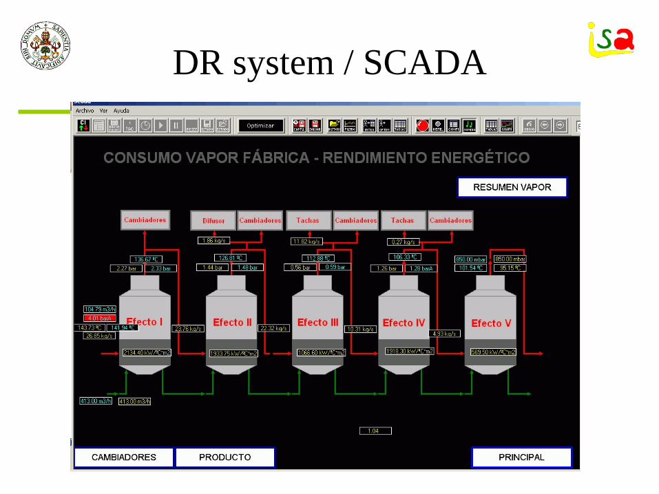
DR system / SCADA

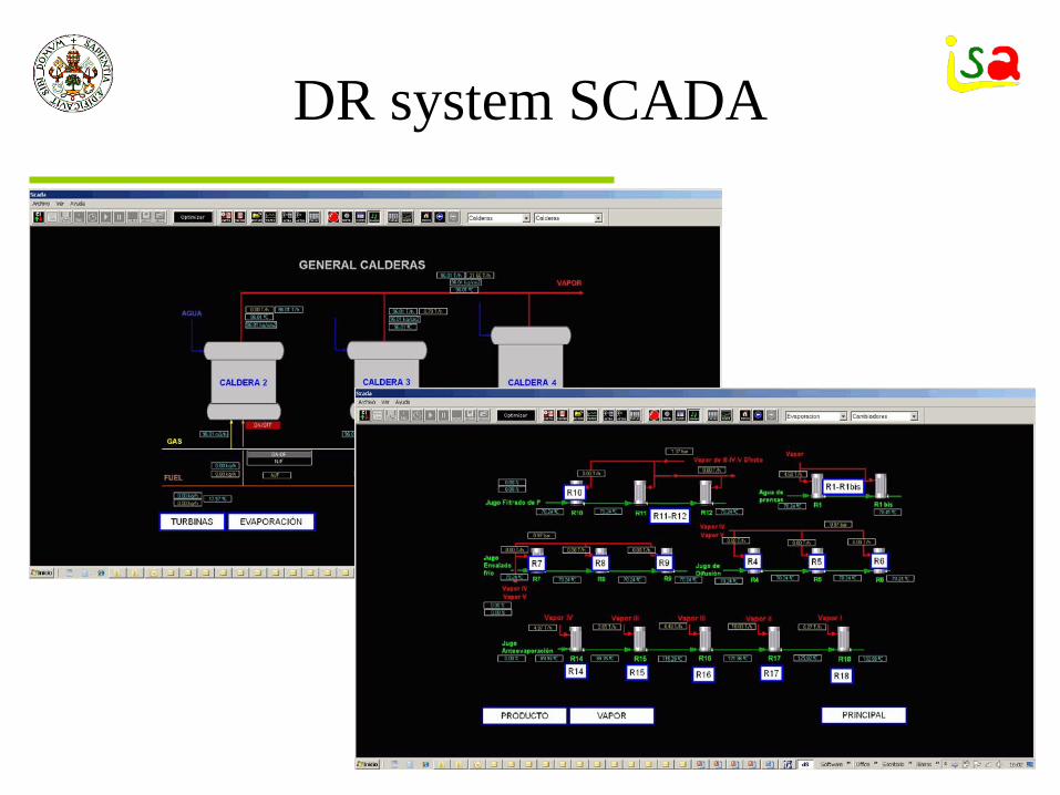
DR system SCADA

Information

Detection of inconsistent measures. Help in fault detection. KPI: Evaluation of energetic behaviour indexes, efficiency,

comparison between process heat transfer coefficients versus theoretical coefficients….

Estimation of all unmeasured variables, some of them relevant for the energy evaluation such as steam consumptions.

Keeping track of the time evolution of key variables during the sugar beet campaign, helping managers in locating malfunctions in the process or equipment fouling and planning maintenance

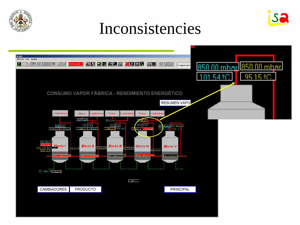
Inconsistencies

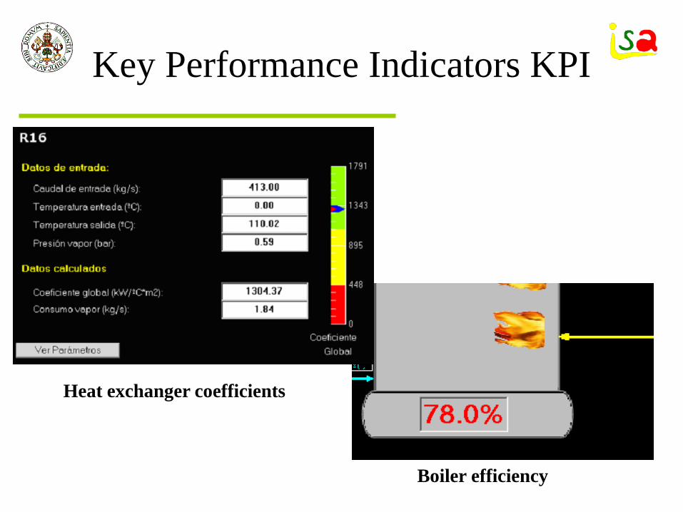
Key Performance Indicators KPI

Heat exchanger coefficients

Boiler efficiency

Hydrogen network

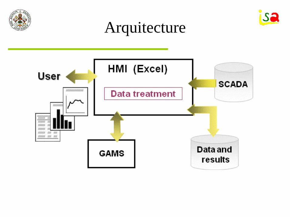
Arquitecture

Data treatmentkey role played by the data treatment in the success of the application in the refinery. If data from the SCADA system are not analyzed and filter previously to their use in the numerical methods, there are no chances to obtain good results. This layer is composed of a set of rules that detect faults and information inconsistences in the raw data and decides which options are the most adequate ones. For instance, detecting when a flow is actually zero, a plant is stopped, a measurement is out of range, etc. It has been developed for specific cases combining physical knowledge and heuristic rules. As a result of these rules, the system adjust the model parameters and optimization weights, so that, e.g. a measurement can be eliminated from the data reconciliation cost function. Mayor changes take place when a plant is not operating. To deal with these cases, the network is formulated as a superstructure that allows to remove groups of equations depending on the value of binary variables that represent the state of the plants.

DR

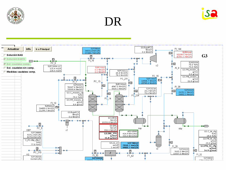
DR

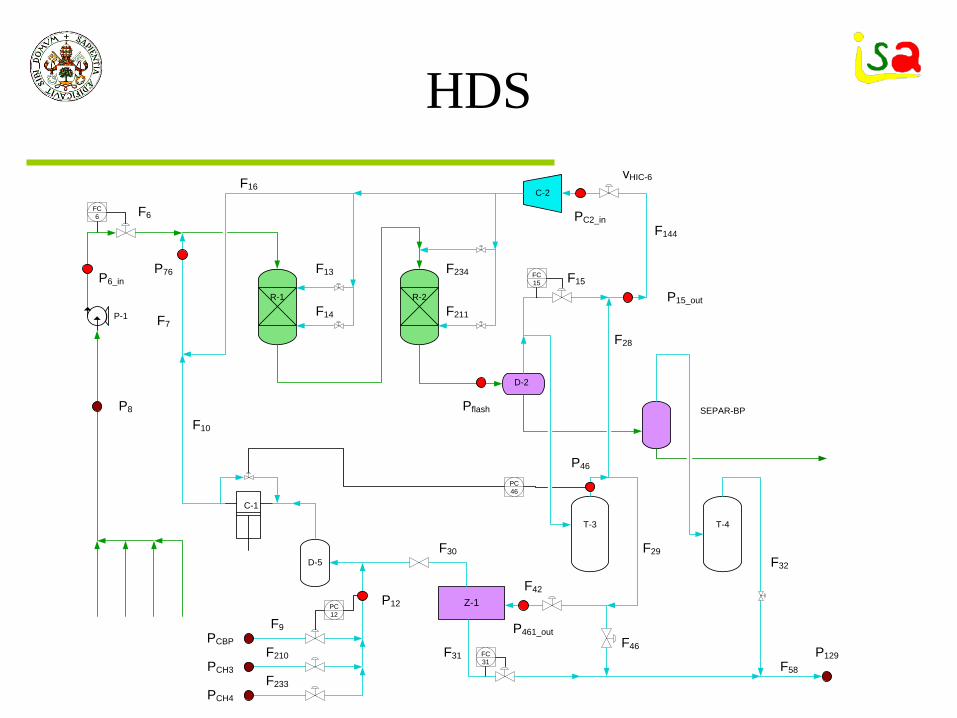
HDS

R-1 R-2

D-2

SEPAR-BP

T-3 T-4

D-5

Z-1

C-2

P76

Pflash

PC2_in

P129

P46

P12

P461_out

F7

F10

F16

F13

F14 F211

F234 F15

F144

F28

F29

F31

F30

F46

F42

F32

F58

F9

F210

F233

P15_out

PCBP

PCH3

PCH4

C-1

P-1

F6

P8

P6_in

vHIC-6

PC46

FC15

FC31

FC6

PC12

DR

Aporte CBP Conc. S salida

Flujo reciclo

Pureza reciclo Pureza BP

Flujo BP

18 days

Conclusions

Data reconciliation is a model based approach to obtain coherent information from the plant.

It allows to compute KPI to follow the time evolution of the process operation.

Formulated as an optimization problem.Open problems:

– Gross error detection– Speed, batch, non-independent variables,…