Embed Size (px)
Citation preview

Olga MoreiraApril 2005
DEA en Sciences“Astérosismologie”
Lectured by Anne Thoul
Data analysis and Its applications Data analysis and Its applications on Asteroseismologyon Asteroseismology

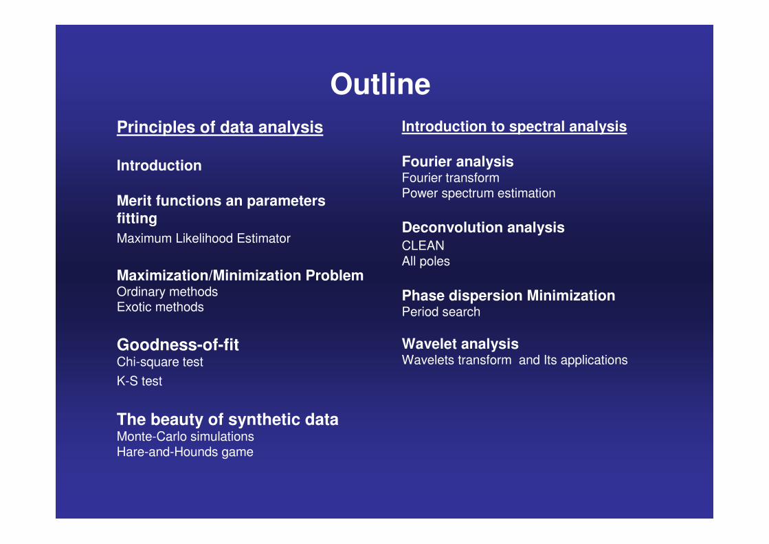
OutlinePrinciples of data analysis
Introduction
Merit functions an parametersfittingMaximum Likelihood Estimator
Maximization/Minimization ProblemOrdinary methodsExotic methods
Goodness-of-fitChi-square testK-S test
The beauty of synthetic dataMonte-Carlo simulationsHare-and-Hounds game
Introduction to spectral analysis
Fourier analysisFourier transformPower spectrum estimation
Deconvolution analysisCLEANAll poles
Phase dispersion MinimizationPeriod search
Wavelet analysisWavelets transform and Its applications

Part IPrinciples of data analysis

Introduction

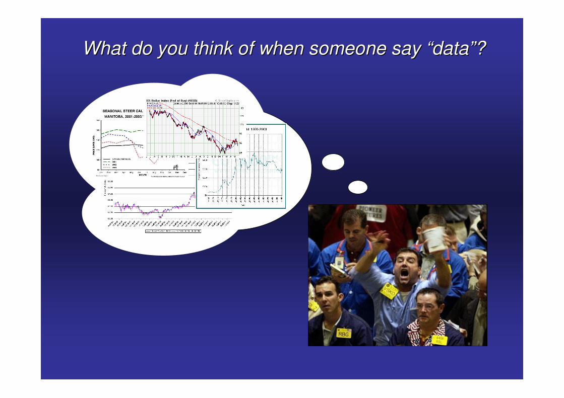
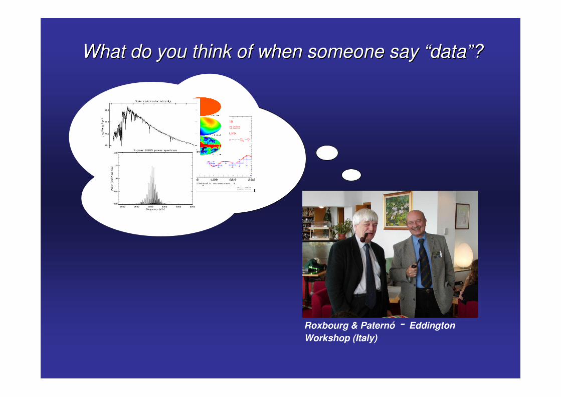
What do you think of when someone say “data”?What do you think of when someone say “data”?
Roxbourg & Paternó - Eddington Workshop (Italy)
What do you think of when someone say “data”?What do you think of when someone say “data”?
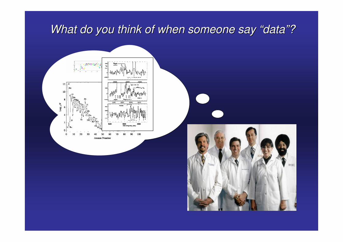
What do you think of when someone say “data”?What do you think of when someone say “data”?

What do you think of when someone say “data”?What do you think of when someone say “data”?

What do you think of when someone say “data”?What do you think of when someone say “data”?
������������������� ����
����������

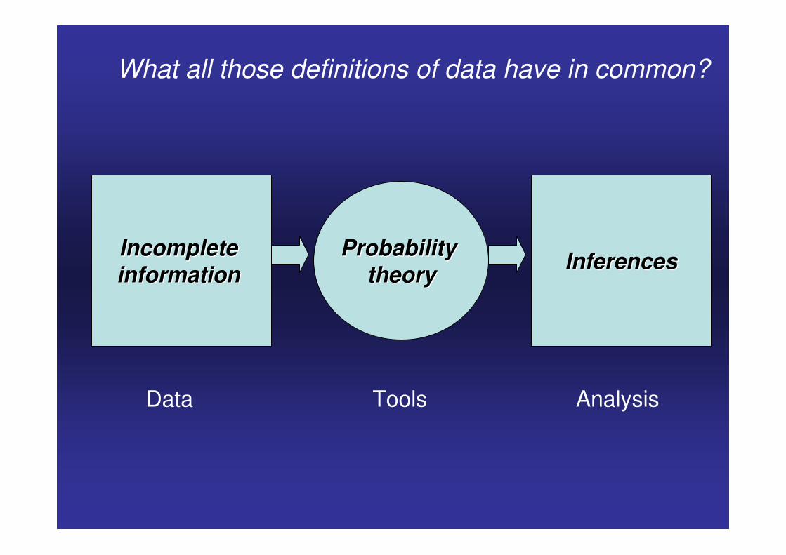
InferencesInferencesProbability Probability theorytheory
Incomplete Incomplete informationinformation
Data Tools Analysis
What all those definitions of data have in common?
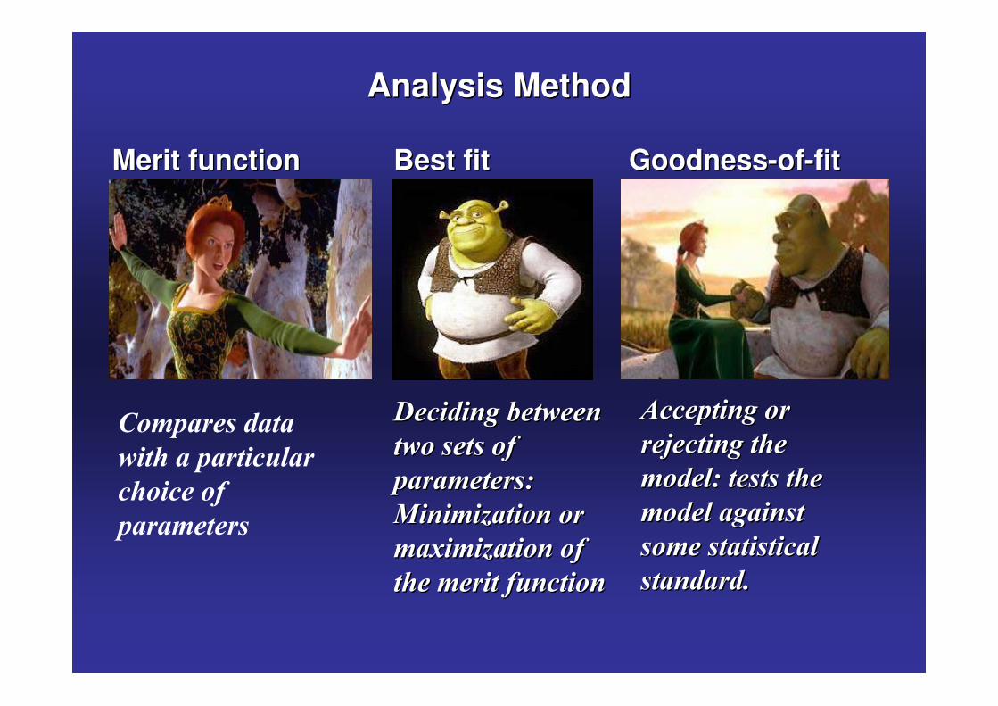
Analysis MethodAnalysis Method
Merit function Merit function
�����������
� ������� �����
��� ����
����������
Best fitBest fit
��� ������������ ���������
������������������
����������������������
� � � ��� ����� � � ��� ����
��� � ��� ������� � ��� ����
������ ������ �������� ������ ��
GoodnessGoodness--ofof--fitfit
������ ���������� ����
������ ����������� �����
��������������������������
������� ���������� ���
�������� �� ����������� �� ���
��������������

Analysis MethodAnalysis Method
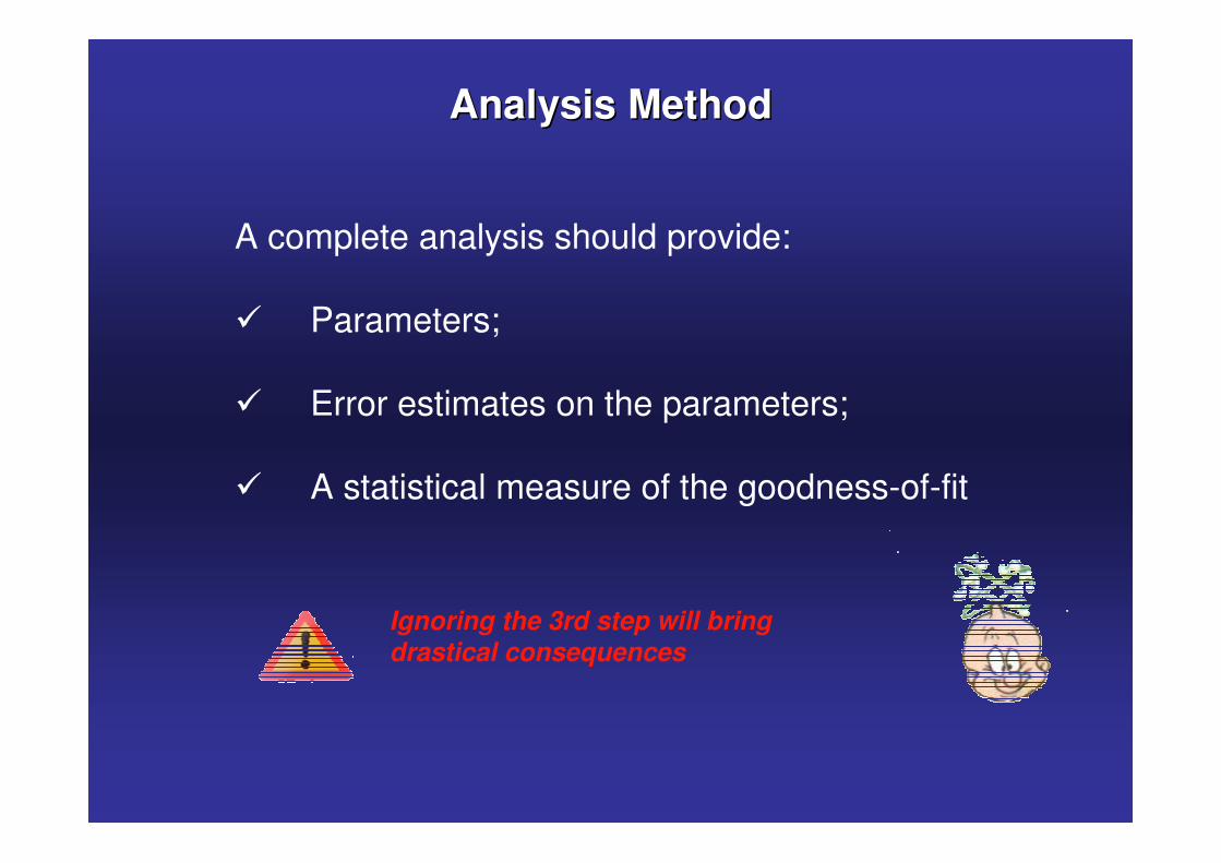
A complete analysis should provide:
� Parameters;
� Error estimates on the parameters;
� A statistical measure of the goodness-of-fit
Ignoring the 3rd step will bring drastical consequences
Merit functions and parameters fitting

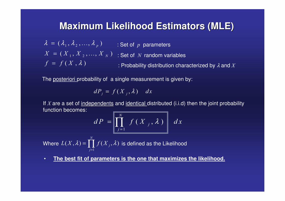
Maximum Likelihood Estimators (MLE)Maximum Likelihood Estimators (MLE)
The posteriori probability of a single measurement is given by:
If � are a set of independents and identical distributed (i.i.d) then the joint probability function becomes:
� � �� ��� � � ��λ=
�
� � ��
�
�
�� � � ��λ=
= ∏
� �
� �
� � � ���� �
� � � ���� �
� � �
�
�� � � �
� � �
λ λ λ λ
λ
=
==
: Set of � parameters
: Set of �random variables
: Probability distribution characterized by λ and �
• The best fit of parameters is the one that maximizes the likelihood.
is defined as the Likelihood�
� � � � � ��
�
�
� � �λ λ=
= ∏Where
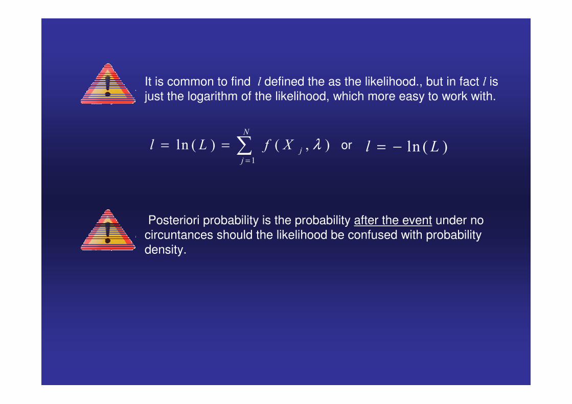
It is common to find � defined the as the likelihood., but in fact � is just the logarithm of the likelihood, which more easy to work with.
�
�� � � � � ��
�
�
� � � λ=
= = � or �� � �� = −
Posteriori probability is the probability after the event under no circuntances should the likelihood be confused with probability density.

���λ�
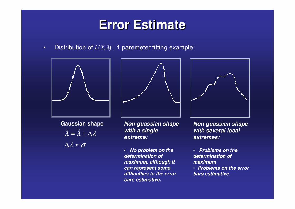
Error EstimateError Estimate
Gaussian shape�λ λ λ
λ σ= ± ∆
∆ ≈
Non-guassian shapewith a single extreme:
• No problem on the determination of maximum, although it can represent some difficulties to the error bars estimative.
Non-guassian shapewith several local extremes:
• Problems on the determination of maximum• Problems on the error bars estimative.
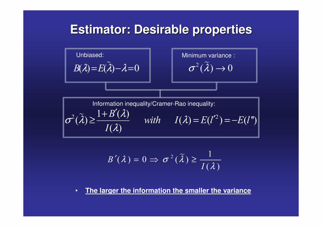
Estimator: Desirable propertiesEstimator: Desirable properties
Unbiased: Minimum variance :
�� � � � �λ λ λ= − = �� � � σ λ →
Information inequality/Cramer-Rao inequality:
�� �� � �� � � � � � � �
� �
���� � � � � �
�
λσ λ λλ′+ ′≥ = = −
• The larger the information the smaller the variance
�� �� � � �
� �
�λ σ λ
λ′ = � ≥
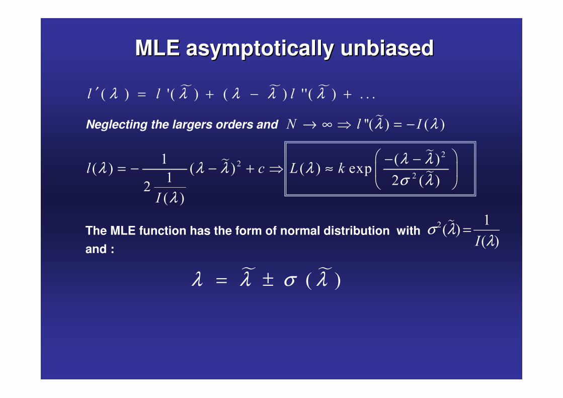
MLE asymptotically unbiasedMLE asymptotically unbiased
� � �� � � � � � � � ���� � �λ λ λ λ λ′ = + − +
Neglecting the largers orders and �� � � �� � �λ λ→ ∞ � = −
��
�
��
�
� � �� � � � � � ��
� � � ��� �
� � �
�
λ λλ λ λ λσ λ
λ
� �− −= − − + � ≈ � �� �
�� �� �
� ��σ λ
λ=The MLE function has the form of normal distribution with
and :
� �� �λ λ σ λ= ±

��
��
� �
� � �
�
� � � �
�
�
� � �
�
� � ����� � � � ����� � � � � � � ��� � � ��
� � � � �� � � � � � � �� �
�
�� � � � � � � �
�
� �� �
�
� � ���
� � �
� � � � � �
� � �� � �
�
�
� � � � ��� � � � � �
� �� �
� � �
�� � � � �
λ λ λ λ λ λ λ
λ λλ λ λ λ λ λ λ λλ λ λ
λ λ λ λ λ λ
λλ λ
=
= = =
= = = =
� � � �∂ ∂= + − − − − +� � � �∂ ∂ ∂� � � �
= + − − +
∂→∞� = =∂ ∂
�
� �� �
�
� �
�
��� � � � �
�
� � �
� � �λ λ λ λ
� �� �� �
� �= − −� �� �
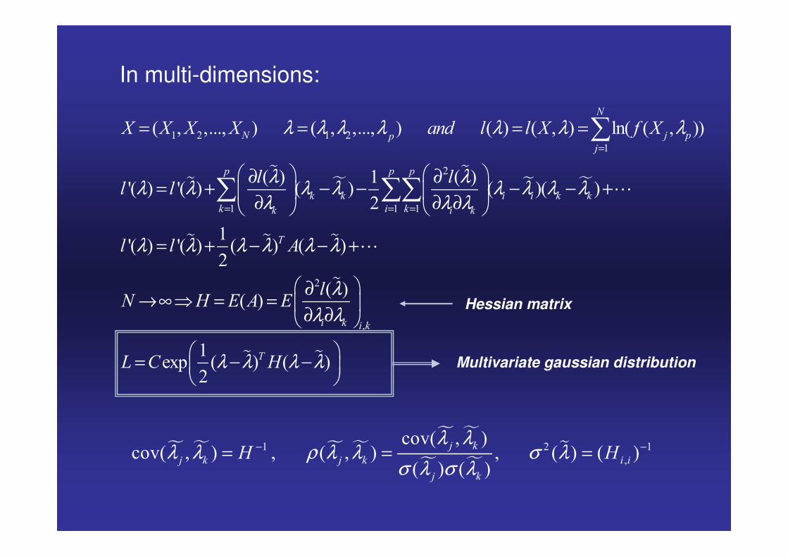
Multivariate gaussian distribution
Hessian matrix
� � � �� �
� �
�� � �
�
���� � ����� � � � � � � � � � � �
� � � �
� �
� � � � � �
� �
� �λ λ
λ λ ρ λ λ σ λσ λ σ λ
− −= = =
In multi-dimensions:

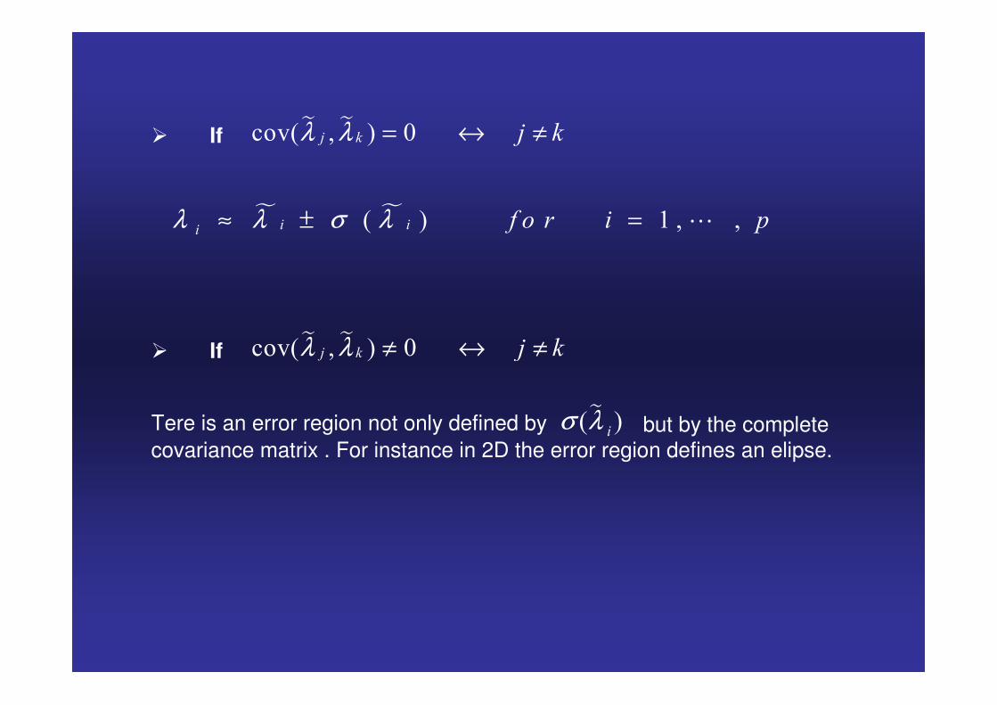
� If � ����� � � � � � �λ λ ≠ ↔ ≠
Tere is an error region not only defined by �� ��σ λ but by the complete covariance matrix . For instance in 2D the error region defines an elipse.
� If � ����� � � � � � �λ λ = ↔ ≠
� �� � � � �� �� � �� � �λ λ σ λ≈ ± = �
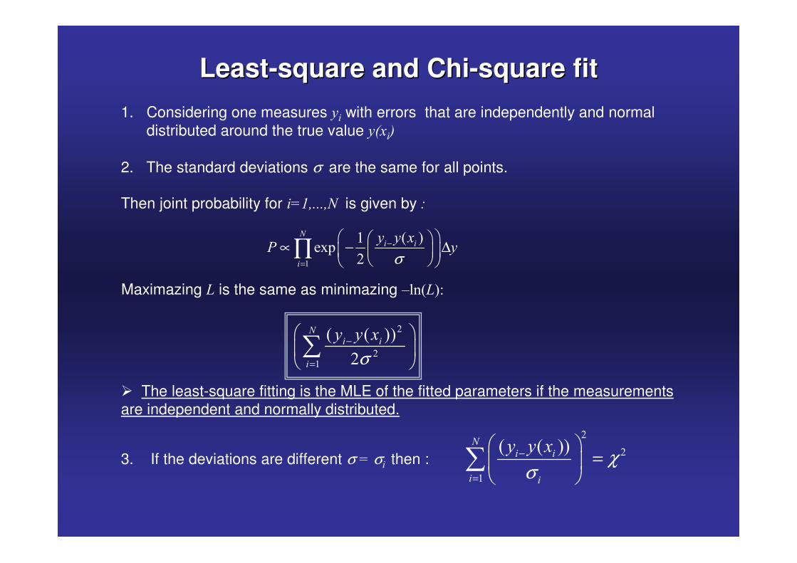
LeastLeast--square and Chisquare and Chi--square fitsquare fit1. Considering one measures �� with errors that are independently and normal
distributed around the true value ����
2. The standard deviations σ are the same for all points.
Then joint probability for �!"�###��is given by $
�
� ����
�
�� �
�
� � �� �
σ−
=
� �� �∝ − ∆� �� �� �� �
∏
Maximazing is the same as minimazing ������
�
��
� � ��
�
�� �
�
� � �
σ−
=
� �� �� ��
� The least-square fitting is the MLE of the fitted parameters if the measurements are independent and normally distributed.
3. If the deviations are different σ !σ� then :
�
�
�
� � ���� �
� �
� � � χσ
−
=
� �=� �
� ��
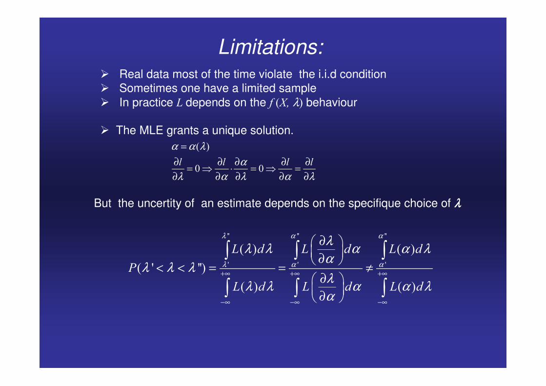
Limitations:� Real data most of the time violate the i.i.d condition� Sometimes one have a limited sample � In practice depends on the ����λ� behaviour
� The MLE grants a unique solution.
But the uncertity of an estimate depends on the specifique choice of λλλλ
� �
� � � �
α α λα
λ α λ α λ
=∂ ∂ ∂ ∂ ∂= � ⋅ = � =∂ ∂ ∂ ∂ ∂
� � � �
� �
� � � �
� � �
�
� � �
λ α α
λ α α
λλ λ α α λα
λ λ λλλ λ α α λα
+∞ +∞ +∞
−∞ −∞ −∞
∂� �� �∂� �< < = = ≠
∂� �� �∂� �

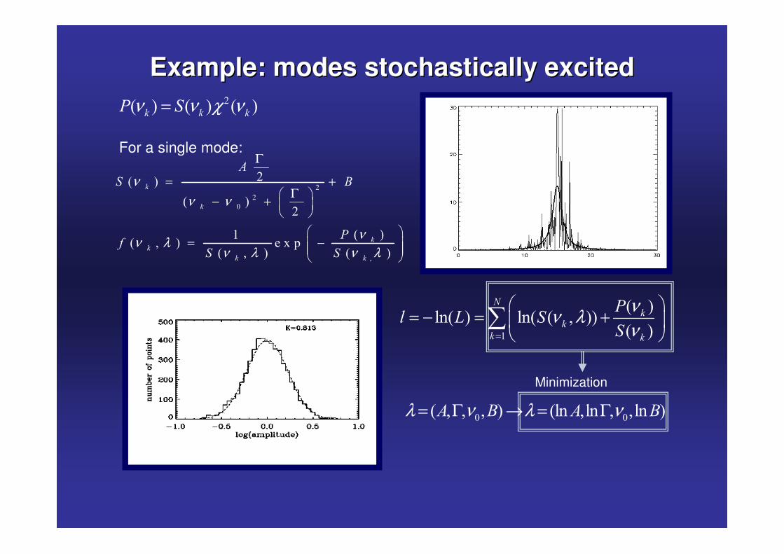
Example: modes stochastically excitedExample: modes stochastically excited�� � � � � �� � �� %ν ν χ ν=
Minimization
For a single mode:
�
�
�
�� �
� ��
� ��� � � ��
� � � � �
�
�
��
� �
�
%
��
% %
νν ν
νν λν λ ν λ
Γ
= +Γ� �− + � �
� �
� �= −� �� �
� �
� � � � � ��� ��� � ��� �� � λ ν λ ν= Γ → = Γ
�
� ���� � ��� � � ��
� �
��
�
� �
�� %
%
νν λν=
� �= − = +� �
� ��

Maximization/Minimization Problem
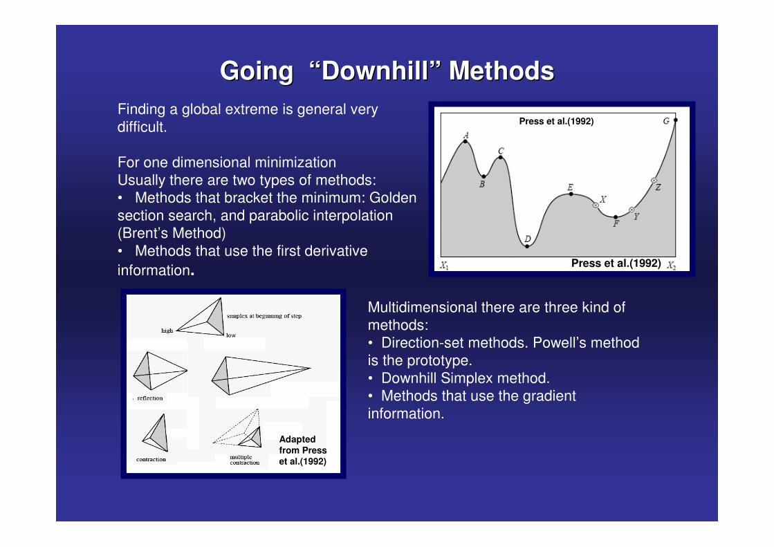
Going “Downhill” MethodsGoing “Downhill” MethodsFinding a global extreme is general very difficult.
For one dimensional minimizationUsually there are two types of methods:• Methods that bracket the minimum: Golden section search, and parabolic interpolation (Brent’s Method)• Methods that use the first derivative information.
Multidimensional there are three kind of methods:• Direction-set methods. Powell’s method is the prototype.• Downhill Simplex method. • Methods that use the gradient information.
Press et al.(1992)
Adapted from Press et al.(1992)
Press et al.(1992)

Falling in the wrong valleyFalling in the wrong valley
The downhill methods a lack on efficiency/robustness. For instance the simplex method can very fast for some functions and very slow for others.
They depend on priori knowledge of the overall structure of vector space, and require repeated manual intervention.
If the function to minimize is not well-known, sometimes, numerically speaking, a smooth hill can become an headache.
They also don’t solve the famous combinatorial analysis problem :The traveling salesman problem
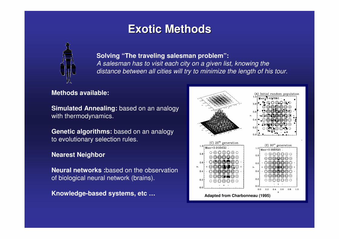
Exotic MethodsExotic Methods
Solving “The traveling salesman problem”:A salesman has to visit each city on a given list, knowing the distance between all cities will try to minimize the length of his tour.
Methods available:
Simulated Annealing: based on an analogy with thermodynamics.
Genetic algorithms: based on an analogy to evolutionary selection rules.
Nearest Neighbor
Neural networks :based on the observation of biological neural network (brains).
Knowledge-based systems, etc … Adapted from Charbonneau (1995)

Goodness-of-fit

ChiChi--square testsquare test
�� !" #$%� &$�"" � '� ��
�( !" #$%" &$� " ( )���
��"* * '����
�+ ! , #$%, ,�������, #+����-��+ #+������
��
�
� ��� �
� �
� �
�χ
=
−=���: is the number of events observed in the ith bin��: is the number expected according to some known distribution
H0: The data follow a specified distribution
Significance level is determined by & is the degree of freedom: &!�'�()*+���+,��)��+�����)+�+�,
Normally acceptable models have -./#//", but day-in and day-out we find accepted models with -!"/'0
�� � �- &χ
� � � � �
� � �
���� � ���
� � � � �� �� � � �
�, +
+
�
�, +
�
1 � - � 1�
� �- � � � ��� �
� �
∞−
=
� � �� �℘ > = + +� � �� � �� �
= − − =+�
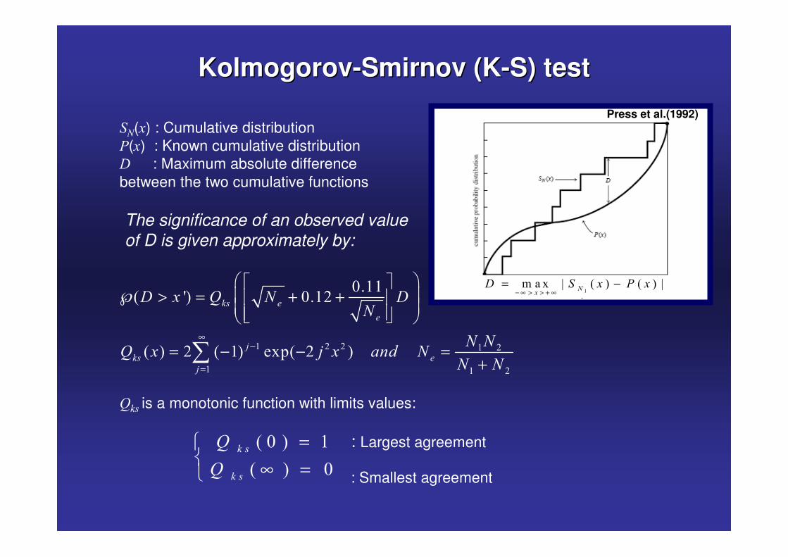
KolmogorovKolmogorov--Smirnov (KSmirnov (K--S) testS) test
%�(�) : Cumulative distribution�(�) : Known cumulative distribution1: Maximum absolute difference between the two cumulative functions
The significance of an observed value of D is given approximately by:
-�, is a monotonic function with limits values:
�� �� � � � � � ��
�1 % � � �
− ∞ > > + ∞= −
Press et al.(1992)
� � �
� �
� ,
� ,
-
-
=�� ∞ =�
: Largest agreement
: Smallest agreement
Synthetic data
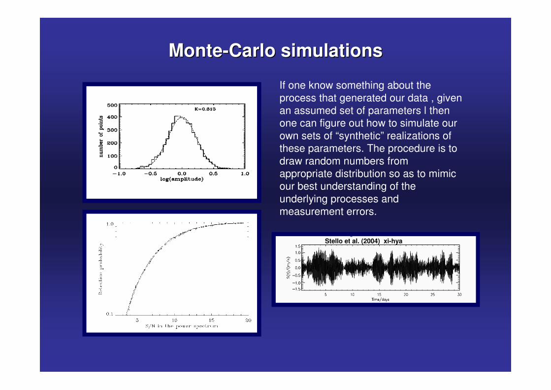
MonteMonte--Carlo simulationsCarlo simulations
If one know something about the process that generated our data , given an assumed set of parameters l then one can figure out how to simulate our own sets of “synthetic” realizations of these parameters. The procedure is to draw random numbers from appropriate distribution so as to mimic our best understanding of the underlying processes and measurement errors.
Stello et al. (2004) xi-hya

HareHare--andand--Hounds gameHounds game
Team A: generates theoretical mode frequencies and synthetic time series.
Team B: analyses the time series, performs the mode identification and fitting, does the structure inversion
Rules: The teams only have access to time series. Nothing else is allowed.

End of Part IOptions available :
• Questions• Coffee break• “Get on with it !!!”

Part II
Introduction to spectral analysis
Fourier transformFourier transform
( )
( )( )
( )
( ) ( )
( )( )
�
� � �� � ��� � � �
� � � � � �
� �� �� � ��
� �
� � � � � � � � � �
� � � � � �
2� � � 2 & � � � &� ��
2� � � 3 � 2 & 4 &
� &2� � 2 & � �� 2 � � � 2
� � � �
� � � � 3 � (�� 2� � � 2 & 4 &
2� � � 3 � 2 & 4 &
π+∞
−∞
+∞
−∞
= =
+ = +
� �� � � �= =� � � �� �� � � �� �
= + ⇔ = ⋅
⊗ = ⋅
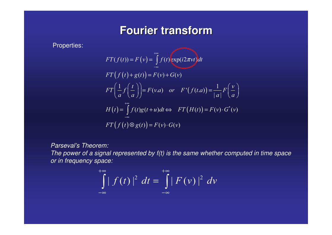
Properties:
Parseval’s Theorem:The power of a signal represented by f(t) is the same whether computed in time space or in frequency space:
� �� � � � � � � �� � �� 2 & �&
+∞ +∞
−∞ −∞
=
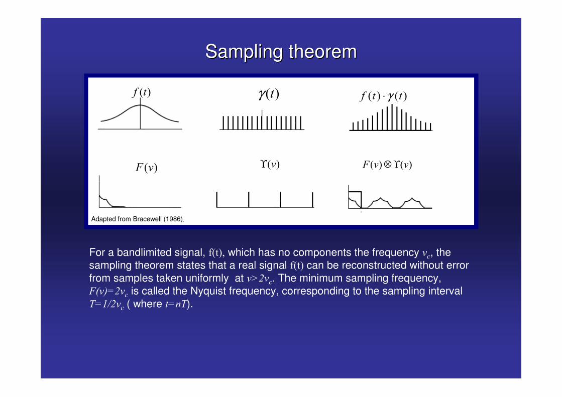
Sampling theoremSampling theorem
For a bandlimited signal, ����� which has no components the frequency &�, the sampling theorem states that a real signal ���� can be reconstructed without error from samples taken uniformly at &.5&�. The minimum sampling frequency, 2�& !5&� is called the Nyquist frequency, corresponding to the sampling interval �!"65&� ( where �!��).
Adapted from Bracewell (1986)
� � � �� � �γ⋅� �� � � ��γ
� �2 & � �&ϒ � � � �2 & &⊗ ϒ

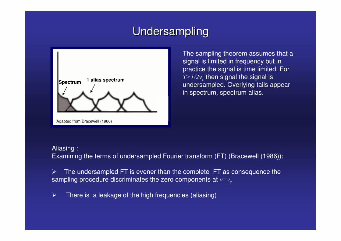
The sampling theorem assumes that a signal is limited in frequency but in practice the signal is time limited. For �."65&� then signal the signal is undersampled. Overlying tails appear in spectrum, spectrum alias.
UndersamplingUndersampling
Adapted from Bracewell (1986)
Spectrum 1 alias spectrum
Aliasing :Examining the terms of undersampled Fourier transform (FT) (Bracewell (1986)):
� The undersampled FT is evener than the complete FT as consequence the sampling procedure discriminates the zero components at &!&�
� There is a leakage of the high frequencies (aliasing)

Discrete Fourier transformDiscrete Fourier transform
�
� � � � �� � � � �� ��
� � � � �
�
2 & � � � & � � � � � �π δ=
= = =� �
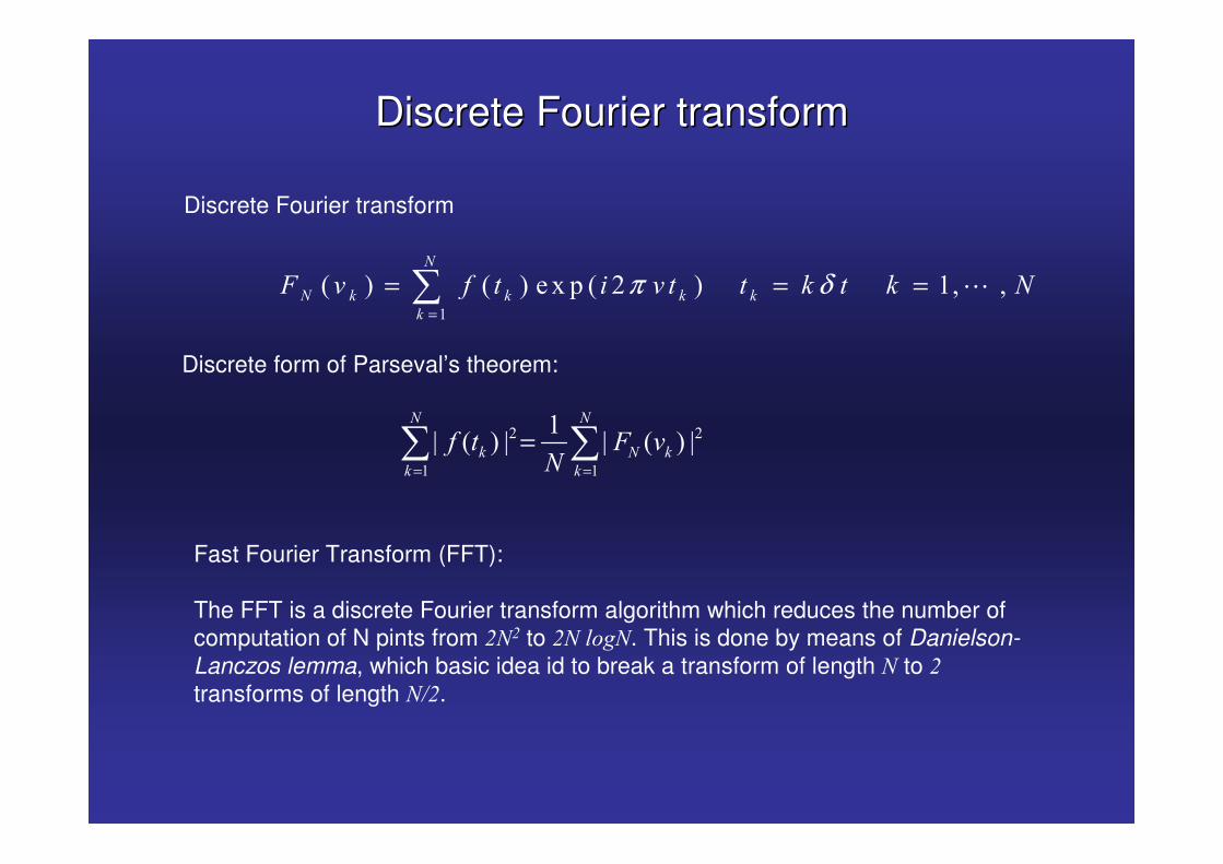
Discrete Fourier transform
� �
� �
�� � �� � � ��
� �
� � �
� �
� � 2 &�= =
=� �
Discrete form of Parseval’s theorem:
Fast Fourier Transform (FFT):
The FFT is a discrete Fourier transform algorithm which reduces the number of computation of N pints from 5�5 to 5���3�. This is done by means of Danielson-Lanczos lemma, which basic idea id to break a transform of length � to 5
transforms of length �65.
Power spectrum estimationPower spectrum estimation
�
�
�
� �
� �
� �� � � � � � �� � � �
�� � � � ����� � � ������ �
�
� �
�
� �
� � � �
� �
� & 2 & � � � &�� �
� & � � &� � � &��
π
π π
=
= =
= =
�� � � �= +� � � � �� � � �� � �
�
� �
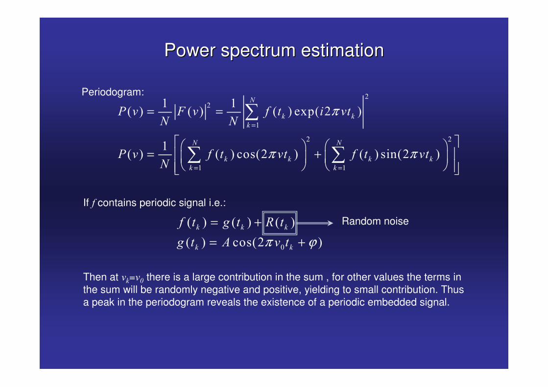
Periodogram:
� � � � � �
� � ����� �
� � �
� �
� � 3 � 7 �
3 � � & �π ϕ= += +
Then at &�=&/ there is a large contribution in the sum , for other values the terms in the sum will be randomly negative and positive, yielding to small contribution. Thus a peak in the periodogram reveals the existence of a periodic embedded signal.
If � contains periodic signal i.e.:
Random noise

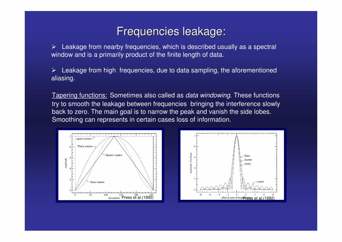
Frequencies leakage:Frequencies leakage:� Leakage from nearby frequencies, which is described usually as a spectral window and is a primarily product of the finite length of data.
� Leakage from high frequencies, due to data sampling, the aforementioned aliasing.
Press et al.(1992) Press et al.(1992)
Tapering functions: Sometimes also called as data windowing. These functions try to smooth the leakage between frequencies bringing the interference slowly back to zero. The main goal is to narrow the peak and vanish the side lobes. Smoothing can represents in certain cases loss of information.
Futher complicationsFuther complications
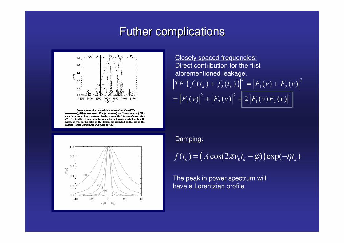
Closely spaced frequencies:Direct contribution for the first aforementioned leakage.
Damping:
( ) � �
� � � �
� �
� � � �
� � � � � � � �
� � � � � � � � �
� ��2 � � � � 2 & 2 &
2 & 2 & 2 & 2 &
+ = +
= + +
( )� � ����� � �� � �� � �� � � & � �π ϕ η= − −
The peak in power spectrum will have a Lorentzian profile

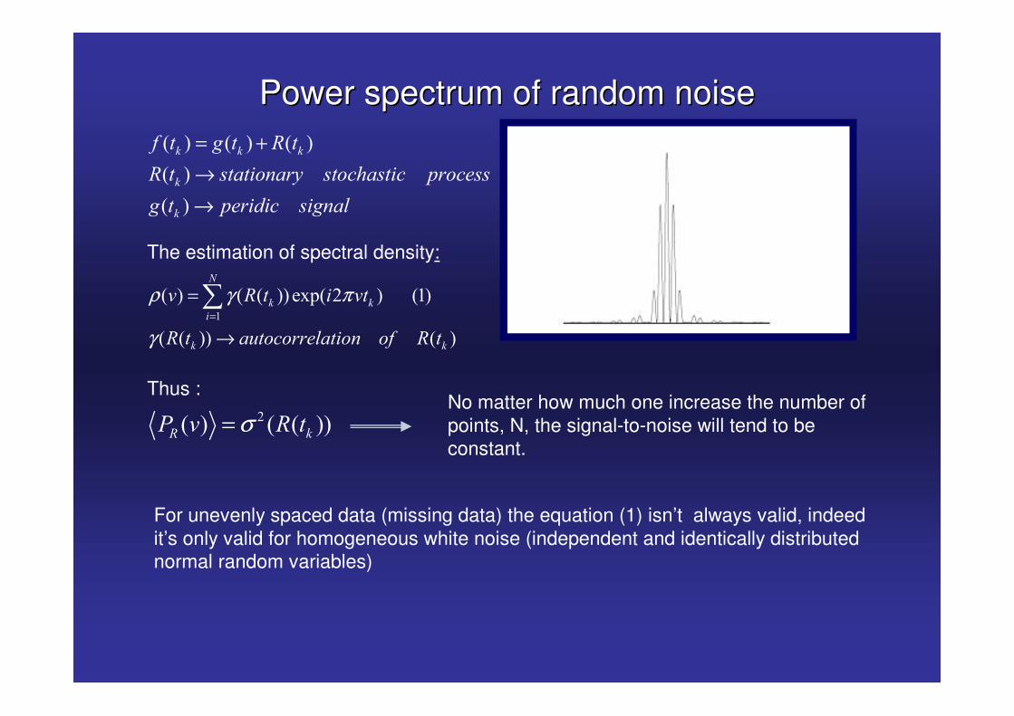
Power spectrum of random noisePower spectrum of random noise� � � � � �
� �
� �
� � �
�
�
� � 3 � 7 �
7 � ,��������� ,�����,��� ����+,,
3 � �+����� ,�3���
= +→→
�
� � � � ���� � � � ���
� � �� � �
�
� �
�
� �
& 7 � � &�
7 � �(������+������ �� 7 �
ρ γ π
γ=
=
→
�
�� � � � ��7 �� & 7 �σ=
The estimation of spectral density:
Thus :No matter how much one increase the number of points, N, the signal-to-noise will tend to be constant.
For unevenly spaced data (missing data) the equation (1) isn’t always valid, indeed it’s only valid for homogeneous white noise (independent and identically distributed normal random variables)

Filling gapsFilling gaps
The unevenly spaced data problem can be solve by (few suggestions):
� Finding a way to reduce the unevenly spaced sample into a evenly spaced.
Basic idea: Interpolation of the missing points (problem: Doesn’t work for long gaps)
� Using the Lomb-Scargle periodogram
� Doing a deconvolution analysis (Filters)

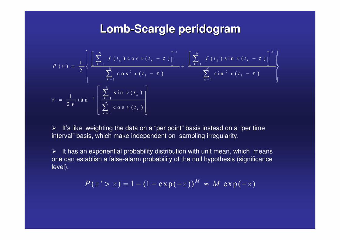
LombLomb--ScargleScargle peridogramperidogram
� �
� �
� �
� �
� �
�
� � ��� � � � � ��� � ��
� ��
��� � � ��� � �
��� � ��
����
��� � �
� �
� � � �
� �
� �
� �
� �
�
�
�
�
�
�
� � & � � � & �
� &
& � & �
& �
&& �
τ τ
τ τ
τ
= =
= =
− =
=
� � � �− −� �� � � �� � � �= +� �� �− −� �� �
�� � =� � � �
� �
� �
�
�
� It’s like weighting the data on a “per point” basis instead on a “per time interval” basis, which make independent on sampling irregularity.
� It has an exponential probability distribution with unit mean, which means one can establish a false-alarm probability of the null hypothesis (significance level).
� � � �� �� � �� �� � �8� 9 9 9 8 9> = − − − ≈ −

Deconvolution analysis
DeconvolutionDeconvolution
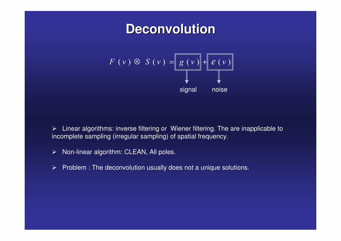
� � � � � � � �2 & % & 3 & &ε⊗ = +
� Linear algorithms: inverse filtering or Wiener filtering. The are inapplicable to incomplete sampling (irregular sampling) of spatial frequency.
� Non-linear algorithm: CLEAN, All poles.
� Problem : The deconvolution usually does not a unique solutions.
noisesignal

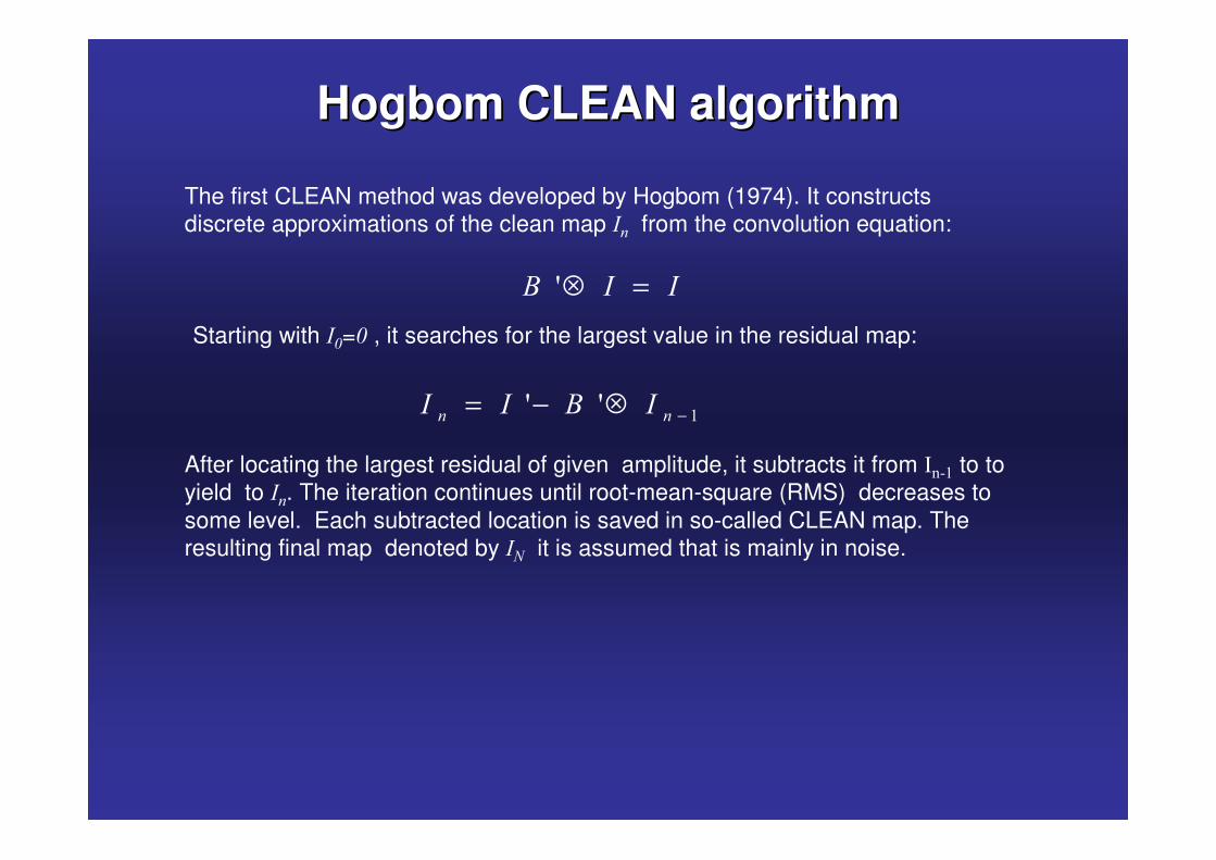
HogbomHogbom CLEAN algorithmCLEAN algorithm
� �⊗ =Starting with �/=/ , it searches for the largest value in the residual map:
The first CLEAN method was developed by Hogbom (1974). It constructs discrete approximations of the clean map �� from the convolution equation:
� � �� � � −= − ⊗
After locating the largest residual of given amplitude, it subtracts it from ���� to toyield to ��. The iteration continues until root-mean-square (RMS) decreases to some level. Each subtracted location is saved in so-called CLEAN map. The resulting final map denoted by �� it is assumed that is mainly in noise.
CLEAN algorithmCLEAN algorithm
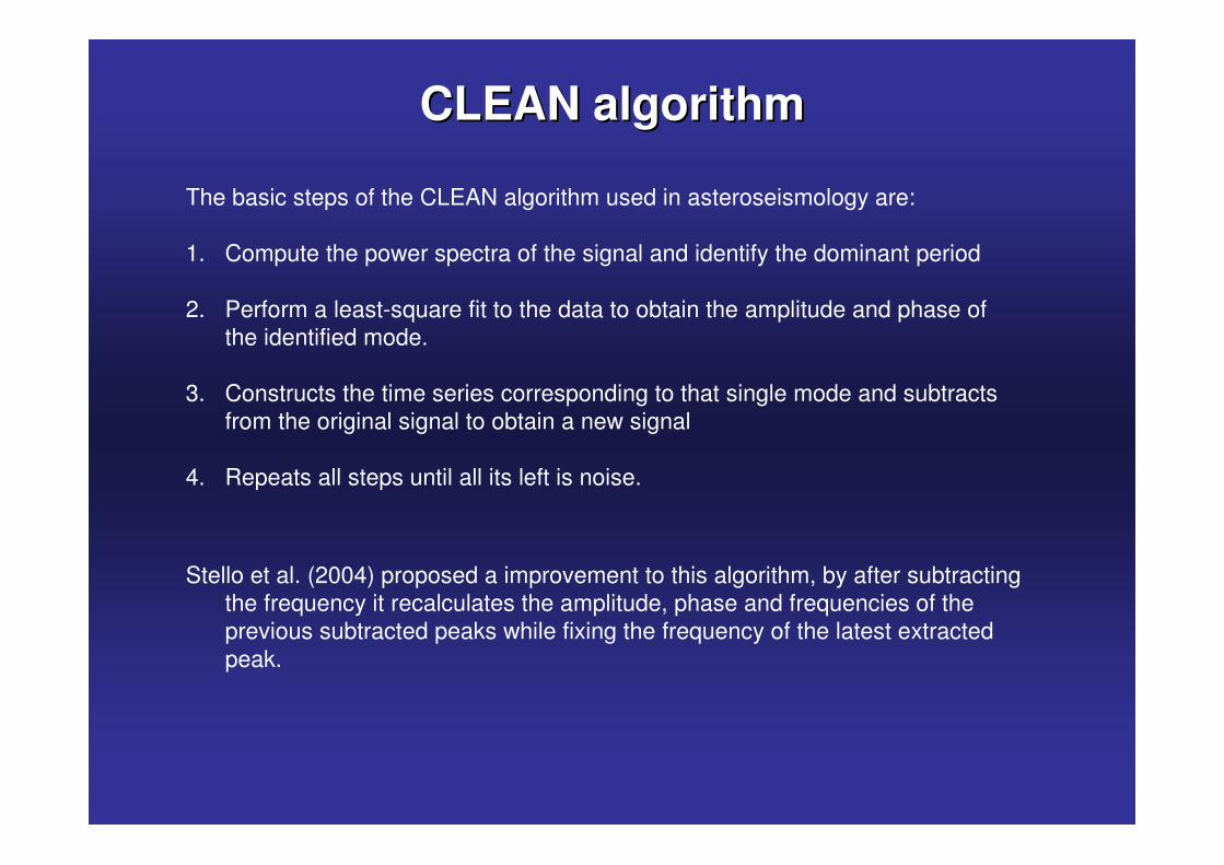
The basic steps of the CLEAN algorithm used in asteroseismology are:
1. Compute the power spectra of the signal and identify the dominant period
2. Perform a least-square fit to the data to obtain the amplitude and phase of the identified mode.
3. Constructs the time series corresponding to that single mode and subtracts from the original signal to obtain a new signal
4. Repeats all steps until all its left is noise.
Stello et al. (2004) proposed a improvement to this algorithm, by after subtracting the frequency it recalculates the amplitude, phase and frequencies of the previous subtracted peaks while fixing the frequency of the latest extracted peak.

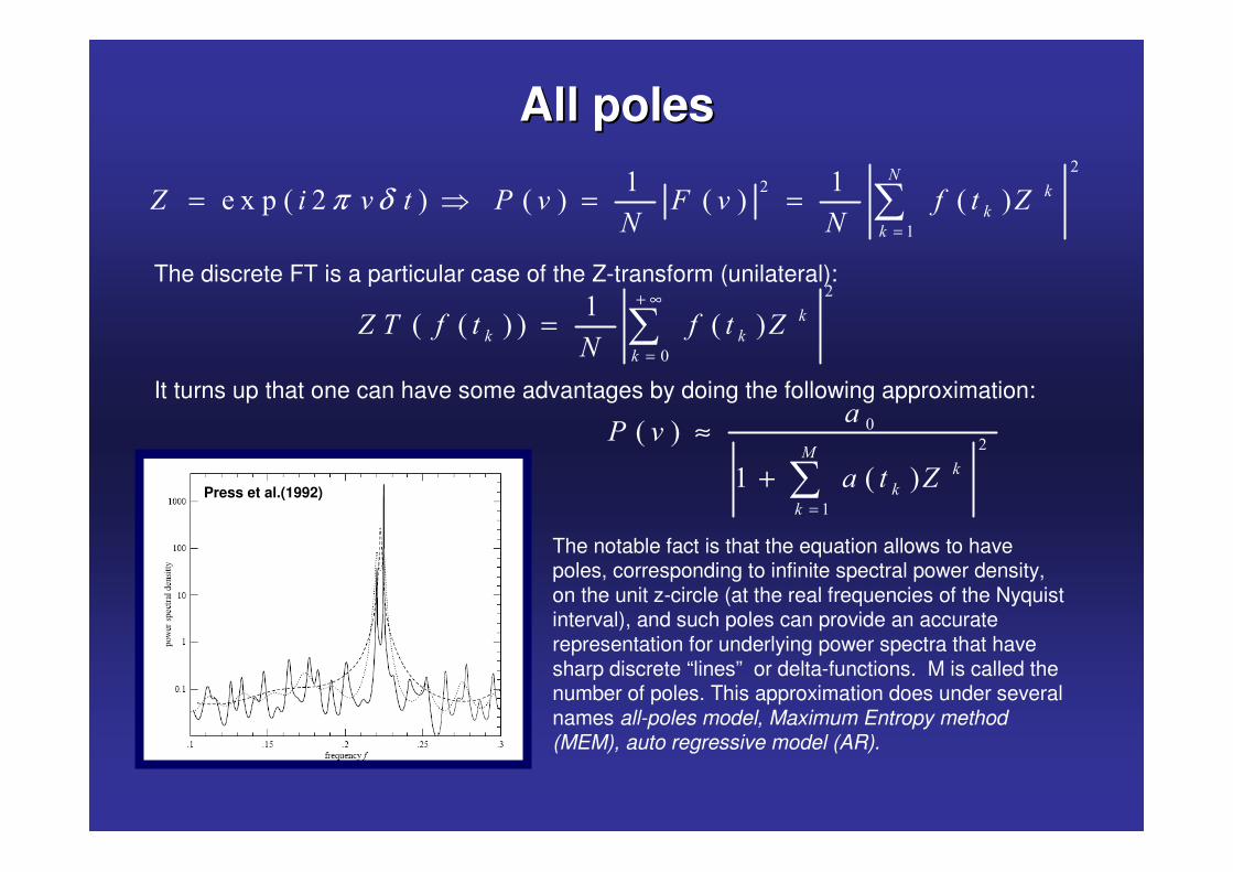
All polesAll poles
The discrete FT is a particular case of the Z-transform (unilateral):
�
�
�
� ��� � � � � � � � � �
��
�
�
: � & � � & 2 & � � :� �
π δ=
= � = = �
�
�� � � � � � �
� �
�
:� � � � � :�
+ ∞
=
= �
�
�
� �
� � �8
�
�
�
�� &
� � :=
≈+ �
It turns up that one can have some advantages by doing the following approximation:
The notable fact is that the equation allows to have poles, corresponding to infinite spectral power density, on the unit z-circle (at the real frequencies of the Nyquistinterval), and such poles can provide an accurate representation for underlying power spectra that have sharp discrete “lines” or delta-functions. M is called the number of poles. This approximation does under several names all-poles model, Maximum Entropy method (MEM), auto regressive model (AR).
Press et al.(1992)

Phase dispersion minimizationPhase dispersion minimization
PDMPDM

DefinitionsDefinitions
�
� �
�
� �
�
�
� �� �
�
� ��
�� �
σ =
=
−= =
−
��
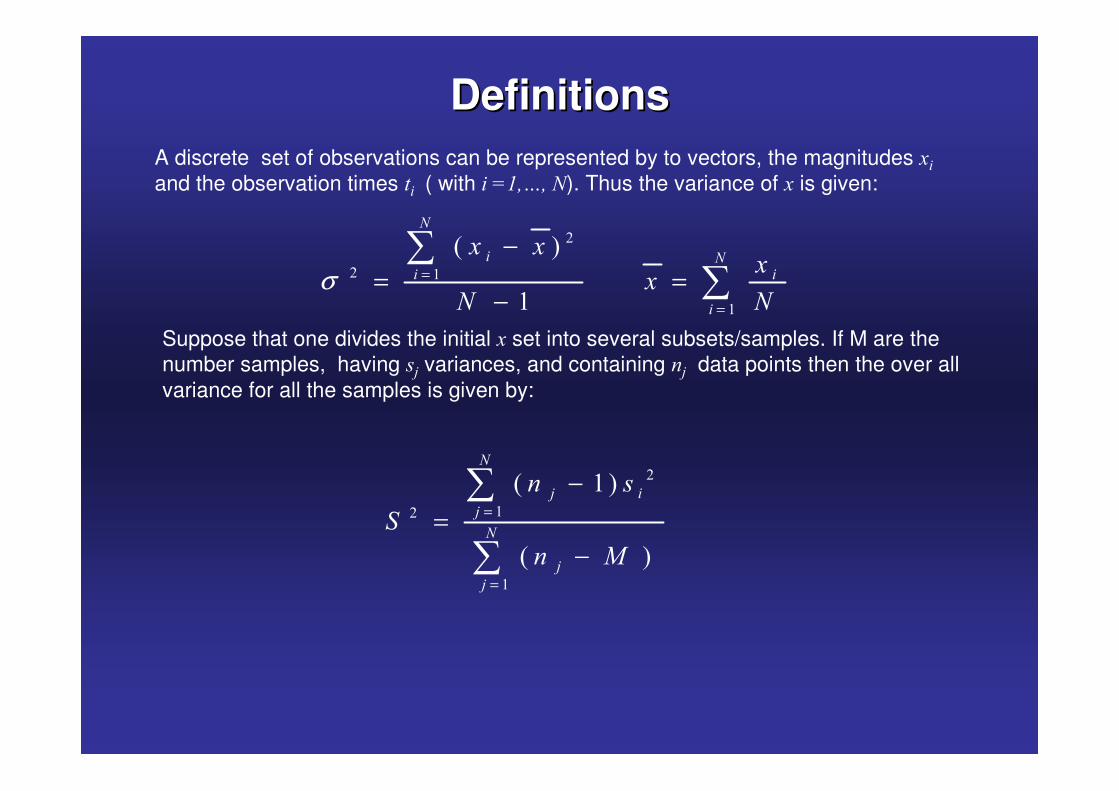
A discrete set of observations can be represented by to vectors, the magnitudes ��
and the observation times �� ( with �!"�;��). Thus the variance of � is given:
Suppose that one divides the initial � set into several subsets/samples. If M are the number samples, having ,� variances, and containing �� data points then the over all variance for all the samples is given by:
�
��
�
� � �
� �
�
� �
�
�
�
�
� ,
%
� 8
=
=
−=
−
�
�
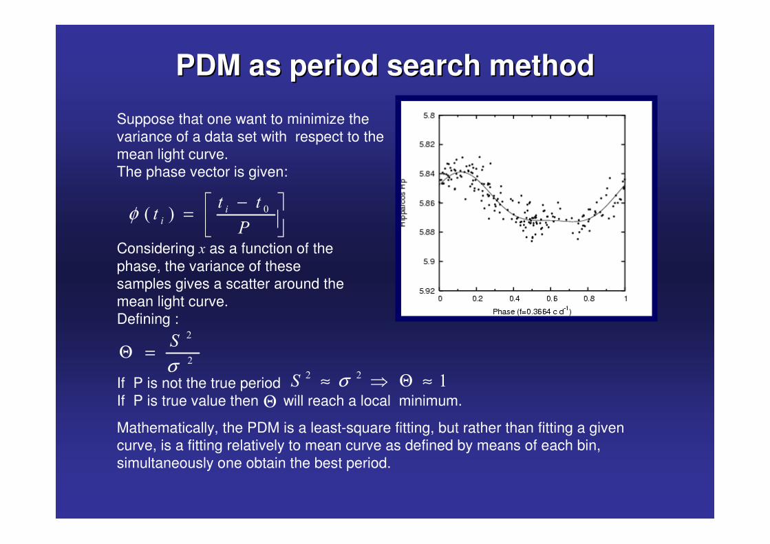
PDM as period search methodPDM as period search method
� � ��
� ��
�φ − �= � � �
Suppose that one want to minimize the variance of a data set with respect to the mean light curve.The phase vector is given:
Considering � as a function of the phase, the variance of these samples gives a scatter around the mean light curve. Defining :
�
�
%
σΘ =
If P is not the true periodIf P is true value then will reach a local minimum.
� � �% σ≈ � Θ ≈Θ
Mathematically, the PDM is a least-square fitting, but rather than fitting a given curve, is a fitting relatively to mean curve as defined by means of each bin, simultaneously one obtain the best period.

WaveletsWavelets

Wavelets transformWavelets transform
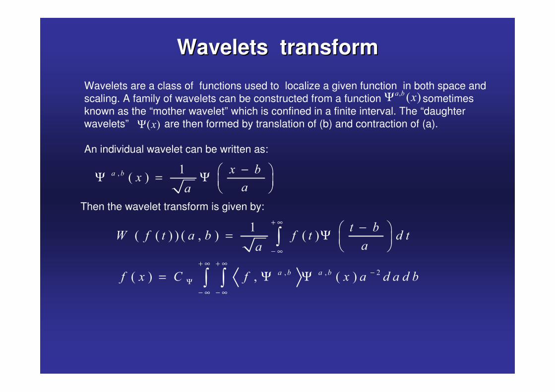
Then the wavelet transform is given by:
� �� �� * � *�
��
−� �Ψ = Ψ � �� �
� � �
�� � � � � � � � �
� � � � �� * � *
� *< � � � * � � ��
��
� � � � � � �� �*
+ ∞
− ∞+ ∞ + ∞
−Ψ
− ∞ − ∞
−� �= Ψ � �� �
= Ψ Ψ
Wavelets are a class of functions used to localize a given function in both space and scaling. A family of wavelets can be constructed from a function sometimes known as the “mother wavelet” which is confined in a finite interval. The “daughter wavelets” are then formed by translation of (b) and contraction of (a).
An individual wavelet can be written as:
� � �� * �Ψ
� ��Ψ
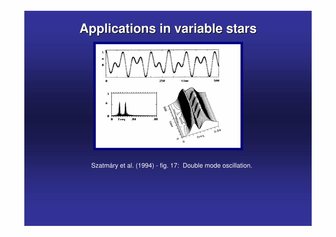
Applications in variable starsApplications in variable stars
Szatmáry et al. (1994) - fig. 17: Double mode oscillation.

Conclusion
Short overviewShort overview
� Data analysis results must never be subjective, it should return the best fitting parameters, the underlying errors, accuracy of the fitted model. All the provided statistical information must be clear.
� Because data is necessary in all scientific fields there a bunch methods for optimization, merit functions, spectral analysis… Therefore, sometimes is not easy to decided which method is the ideal method. Most of the time it the decision dependents on the data to be analyzed.
� All that has been considering here, was the case of a deterministic signal (a fixed amplitude) add to random noise. Sometimes the signal itself is probabilistic
Olga MoreiraApril 2005
DEA en Sciences“Astérosismologie”
Lectured by Anne Thoul
Data analysis and Its applications Data analysis and Its applications on Asteroseismologyon Asteroseismology
OutlinePrinciples of data analysis
Introduction
Merit functions an parametersfittingMaximum Likelihood Estimator
Maximization/Minimization ProblemOrdinary methodsExotic methods
Goodness-of-fitChi-square testK-S test
The beauty of synthetic dataMonte-Carlo simulationsHare-and-Hounds game
Introduction to spectral analysis
Fourier analysisFourier transformPower spectrum estimation
Deconvolution analysisCLEANAll poles
Phase dispersion MinimizationPeriod search
Wavelet analysisWavelets transform and Its applications
Part IPrinciples of data analysis

Introduction
What do you think of when someone say “data”?What do you think of when someone say “data”?
Roxbourg & Paternó - Eddington Workshop (Italy)

What do you think of when someone say “data”?What do you think of when someone say “data”?

What do you think of when someone say “data”?What do you think of when someone say “data”?

What do you think of when someone say “data”?What do you think of when someone say “data”?

What do you think of when someone say “data”?What do you think of when someone say “data”?
������������������� ����
����������
InferencesInferencesProbability Probability theorytheory
Incomplete Incomplete informationinformation
Data Tools Analysis
What all those definitions of data have in common?

Analysis MethodAnalysis Method
Merit function Merit function
�����������
� ������� �����
��� ����
����������
Best fitBest fit
��� ������������ ���������
������������������
����������������������
� � � ��� ����� � � ��� ����
��� � ��� ������� � ��� ����
������ ������ �������� ������ ��
GoodnessGoodness--ofof--fitfit
������ ���������� ����
������ ����������� �����
��������������������������
������� ���������� ���
�������� �� ����������� �� ���
��������������
Analysis MethodAnalysis Method
A complete analysis should provide:
� Parameters;
� Error estimates on the parameters;
� A statistical measure of the goodness-of-fit
Ignoring the 3rd step will bring drastical consequences

Merit functions and parameters fitting
Maximum Likelihood Estimators (MLE)Maximum Likelihood Estimators (MLE)
The posteriori probability of a single measurement is given by:
If � are a set of independents and identical distributed (i.i.d) then the joint probability function becomes:
� � �� ��� � � ��λ=
�
� � ��
�
�
�� � � ��λ=
= ∏
� �
� �
� � � ���� �
� � � ���� �
� � �
�
�� � � �
� � �
λ λ λ λ
λ
=
==
: Set of � parameters
: Set of �random variables
: Probability distribution characterized by λ and �
• The best fit of parameters is the one that maximizes the likelihood.
is defined as the Likelihood�
� � � � � ��
�
�
� � �λ λ=
= ∏Where

It is common to find � defined the as the likelihood., but in fact � is just the logarithm of the likelihood, which more easy to work with.
�
�� � � � � ��
�
�
� � � λ=
= = � or �� � �� = −
Posteriori probability is the probability after the event under no circuntances should the likelihood be confused with probability density.
���λ�
Error EstimateError Estimate
Gaussian shape�λ λ λ
λ σ= ± ∆
∆ ≈
Non-guassian shapewith a single extreme:
• No problem on the determination of maximum, although it can represent some difficulties to the error bars estimative.
Non-guassian shapewith several local extremes:
• Problems on the determination of maximum• Problems on the error bars estimative.

Estimator: Desirable propertiesEstimator: Desirable properties
Unbiased: Minimum variance :
�� � � � �λ λ λ= − = �� � � σ λ →
Information inequality/Cramer-Rao inequality:
�� �� � �� � � � � � � �
� �
���� � � � � �
�
λσ λ λλ′+ ′≥ = = −
• The larger the information the smaller the variance
�� �� � � �
� �
�λ σ λ
λ′ = � ≥

MLE asymptotically unbiasedMLE asymptotically unbiased
� � �� � � � � � � � ���� � �λ λ λ λ λ′ = + − +
Neglecting the largers orders and �� � � �� � �λ λ→ ∞ � = −
��
�
��
�
� � �� � � � � � ��
� � � ��� �
� � �
�
λ λλ λ λ λσ λ
λ
� �− −= − − + � ≈ � �� �
�� �� �
� ��σ λ
λ=The MLE function has the form of normal distribution with
and :
� �� �λ λ σ λ= ±
��
��
� �
� � �
�
� � � �
�
�
� � �
�
� � ����� � � � ����� � � � � � � ��� � � ��
� � � � �� � � � � � � �� �
�
�� � � � � � � �
�
� �� �
�
� � ���
� � �
� � � � � �
� � �� � �
�
�
� � � � ��� � � � � �
� �� �
� � �
�� � � � �
λ λ λ λ λ λ λ
λ λλ λ λ λ λ λ λ λλ λ λ
λ λ λ λ λ λ
λλ λ
=
= = =
= = = =
� � � �∂ ∂= + − − − − +� � � �∂ ∂ ∂� � � �
= + − − +
∂→∞� = =∂ ∂
�
� �� �
�
� �
�
��� � � � �
�
� � �
� � �λ λ λ λ
� �� �� �
� �= − −� �� �
Multivariate gaussian distribution
Hessian matrix
� � � �� �
� �
�� � �
�
���� � ����� � � � � � � � � � � �
� � � �
� �
� � � � � �
� �
� �λ λ
λ λ ρ λ λ σ λσ λ σ λ
− −= = =
In multi-dimensions:
� If � ����� � � � � � �λ λ ≠ ↔ ≠
Tere is an error region not only defined by �� ��σ λ but by the complete covariance matrix . For instance in 2D the error region defines an elipse.
� If � ����� � � � � � �λ λ = ↔ ≠
� �� � � � �� �� � �� � �λ λ σ λ≈ ± = �

LeastLeast--square and Chisquare and Chi--square fitsquare fit1. Considering one measures �� with errors that are independently and normal
distributed around the true value ����
2. The standard deviations σ are the same for all points.
Then joint probability for �!"�###��is given by $
�
� ����
�
�� �
�
� � �� �
σ−
=
� �� �∝ − ∆� �� �� �� �
∏
Maximazing is the same as minimazing ������
�
��
� � ��
�
�� �
�
� � �
σ−
=
� �� �� ��
� The least-square fitting is the MLE of the fitted parameters if the measurements are independent and normally distributed.
3. If the deviations are different σ !σ� then :
�
�
�
� � ���� �
� �
� � � χσ
−
=
� �=� �
� ��

Limitations:� Real data most of the time violate the i.i.d condition� Sometimes one have a limited sample � In practice depends on the ����λ� behaviour
� The MLE grants a unique solution.
But the uncertity of an estimate depends on the specifique choice of λλλλ
� �
� � � �
α α λα
λ α λ α λ
=∂ ∂ ∂ ∂ ∂= � ⋅ = � =∂ ∂ ∂ ∂ ∂
� � � �
� �
� � � �
� � �
�
� � �
λ α α
λ α α
λλ λ α α λα
λ λ λλλ λ α α λα
+∞ +∞ +∞
−∞ −∞ −∞
∂� �� �∂� �< < = = ≠
∂� �� �∂� �
Example: modes stochastically excitedExample: modes stochastically excited�� � � � � �� � �� %ν ν χ ν=
Minimization
For a single mode:
�
�
�
�� �
� ��
� ��� � � ��
� � � � �
�
�
��
� �
�
%
��
% %
νν ν
νν λν λ ν λ
Γ
= +Γ� �− + � �
� �
� �= −� �� �
� �
� � � � � ��� ��� � ��� �� � λ ν λ ν= Γ → = Γ
�
� ���� � ��� � � ��
� �
��
�
� �
�� %
%
νν λν=
� �= − = +� �
� ��

Maximization/Minimization Problem

Going “Downhill” MethodsGoing “Downhill” MethodsFinding a global extreme is general very difficult.
For one dimensional minimizationUsually there are two types of methods:• Methods that bracket the minimum: Golden section search, and parabolic interpolation (Brent’s Method)• Methods that use the first derivative information.
Multidimensional there are three kind of methods:• Direction-set methods. Powell’s method is the prototype.• Downhill Simplex method. • Methods that use the gradient information.
Press et al.(1992)
Adapted from Press et al.(1992)
Press et al.(1992)

Falling in the wrong valleyFalling in the wrong valley
The downhill methods a lack on efficiency/robustness. For instance the simplex method can very fast for some functions and very slow for others.
They depend on priori knowledge of the overall structure of vector space, and require repeated manual intervention.
If the function to minimize is not well-known, sometimes, numerically speaking, a smooth hill can become an headache.
They also don’t solve the famous combinatorial analysis problem :The traveling salesman problem

Exotic MethodsExotic Methods
Solving “The traveling salesman problem”:A salesman has to visit each city on a given list, knowing the distance between all cities will try to minimize the length of his tour.
Methods available:
Simulated Annealing: based on an analogy with thermodynamics.
Genetic algorithms: based on an analogy to evolutionary selection rules.
Nearest Neighbor
Neural networks :based on the observation of biological neural network (brains).
Knowledge-based systems, etc … Adapted from Charbonneau (1995)

Goodness-of-fit

ChiChi--square testsquare test
�� !" #$%� &$�"" � '� ��
�( !" #$%" &$� " ( )���
��"* * '����
�+ ! , #$%, ,�������, #+����-��+ #+������
��
�
� ��� �
� �
� �
�χ
=
−=���: is the number of events observed in the ith bin��: is the number expected according to some known distribution
H0: The data follow a specified distribution
Significance level is determined by & is the degree of freedom: &!�'�()*+���+,��)��+�����)+�+�,
Normally acceptable models have -./#//", but day-in and day-out we find accepted models with -!"/'0
�� � �- &χ

� � � � �
� � �
���� � ���
� � � � �� �� � � �
�, +
+
�
�, +
�
1 � - � 1�
� �- � � � ��� �
� �
∞−
=
� � �� �℘ > = + +� � �� � �� �
= − − =+�
KolmogorovKolmogorov--Smirnov (KSmirnov (K--S) testS) test
%�(�) : Cumulative distribution�(�) : Known cumulative distribution1: Maximum absolute difference between the two cumulative functions
The significance of an observed value of D is given approximately by:
-�, is a monotonic function with limits values:
�� �� � � � � � ��
�1 % � � �
− ∞ > > + ∞= −
Press et al.(1992)
� � �
� �
� ,
� ,
-
-
=�� ∞ =�
: Largest agreement
: Smallest agreement

Synthetic data

MonteMonte--Carlo simulationsCarlo simulations
If one know something about the process that generated our data , given an assumed set of parameters l then one can figure out how to simulate our own sets of “synthetic” realizations of these parameters. The procedure is to draw random numbers from appropriate distribution so as to mimic our best understanding of the underlying processes and measurement errors.
Stello et al. (2004) xi-hya

HareHare--andand--Hounds gameHounds game
Team A: generates theoretical mode frequencies and synthetic time series.
Team B: analyses the time series, performs the mode identification and fitting, does the structure inversion
Rules: The teams only have access to time series. Nothing else is allowed.

End of Part IOptions available :
• Questions• Coffee break• “Get on with it !!!”

Part II
Introduction to spectral analysis

Fourier transformFourier transform
( )
( )( )
( )
( ) ( )
( )( )
�
� � �� � ��� � � �
� � � � � �
� �� �� � ��
� �
� � � � � � � � � �
� � � � � �
2� � � 2 & � � � &� ��
2� � � 3 � 2 & 4 &
� &2� � 2 & � �� 2 � � � 2
� � � �
� � � � 3 � (�� 2� � � 2 & 4 &
2� � � 3� 2 & 4 &
π+∞
−∞
+∞
−∞
= =
+ = +
� �� � � �= =� � � �� �� � � �� �
= + ⇔ = ⋅
⊗ = ⋅
Properties:
Parseval’s Theorem:The power of a signal represented by f(t) is the same whether computed in time space or in frequency space:
� �� � � � � � � �� � �� 2 & �&
+∞ +∞
−∞ −∞
=

Sampling theoremSampling theorem
For a bandlimited signal, ����� which has no components the frequency &�, the sampling theorem states that a real signal ���� can be reconstructed without error from samples taken uniformly at &.5&�. The minimum sampling frequency, 2�& !5&� is called the Nyquist frequency, corresponding to the sampling interval �!"65&� ( where �!��).
Adapted from Bracewell (1986)
� � � �� � �γ⋅� �� � � ��γ
� �2 & � �&ϒ � � � �2 & &⊗ ϒ
The sampling theorem assumes that a signal is limited in frequency but in practice the signal is time limited. For �."65&� then signal the signal is undersampled. Overlying tails appear in spectrum, spectrum alias.
UndersamplingUndersampling
Adapted from Bracewell (1986)
Spectrum 1 alias spectrum
Aliasing :Examining the terms of undersampled Fourier transform (FT) (Bracewell (1986)):
� The undersampled FT is evener than the complete FT as consequence the sampling procedure discriminates the zero components at &!&�
� There is a leakage of the high frequencies (aliasing)
Discrete Fourier transformDiscrete Fourier transform
�
� � � � �� � � � �� ��
� � � � �
�
2 & � � � & � � � � � �π δ=
= = =� �
Discrete Fourier transform
� �
� �
�� � �� � � ��
� �
� � �
� �
� � 2 &�= =
=� �
Discrete form of Parseval’s theorem:
Fast Fourier Transform (FFT):
The FFT is a discrete Fourier transform algorithm which reduces the number of computation of N pints from 5�5 to 5���3�. This is done by means of Danielson-Lanczos lemma, which basic idea id to break a transform of length � to 5
transforms of length �65.

Power spectrum estimationPower spectrum estimation
�
�
�
� �
� �
� �� � � � � � �� � � �
�� � � � ����� � � ������ �
�
� �
�
� �
� � � �
� �
� & 2 & � � � &�� �
� & � � &� � � &��
π
π π
=
= =
= =
�� � � �= +� � � � �� � � �� � �
�
� �
Periodogram:
� � � � � �
� � ����� �
� � �
� �
� � 3 � 7 �
3 � � & �π ϕ= += +
Then at &�=&/ there is a large contribution in the sum , for other values the terms in the sum will be randomly negative and positive, yielding to small contribution. Thus a peak in the periodogram reveals the existence of a periodic embedded signal.
If � contains periodic signal i.e.:
Random noise
Frequencies leakage:Frequencies leakage:� Leakage from nearby frequencies, which is described usually as a spectral window and is a primarily product of the finite length of data.
� Leakage from high frequencies, due to data sampling, the aforementioned aliasing.
Press et al.(1992) Press et al.(1992)
Tapering functions: Sometimes also called as data windowing. These functions try to smooth the leakage between frequencies bringing the interference slowly back to zero. The main goal is to narrow the peak and vanish the side lobes. Smoothing can represents in certain cases loss of information.

Futher complicationsFuther complications
Closely spaced frequencies:Direct contribution for the first aforementioned leakage.
Damping:
( ) � �
� � � �
� �
� � � �
� � � � � � � �
� � � � � � � � �
� ��2 � � � � 2 & 2 &
2 & 2 & 2 & 2 &
+ = +
= + +
( )� � ����� � �� � �� � �� � � & � �π ϕ η= − −
The peak in power spectrum will have a Lorentzian profile
Power spectrum of random noisePower spectrum of random noise� � � � � �
� �
� �
� � �
�
�
� � 3 � 7 �
7 � ,��������� ,�����,��� ����+,,
3 � �+����� ,�3���
= +→→
�
� � � � ���� � � � ���
� � �� � �
�
� �
�
� �
& 7 � � &�
7 � �(������+������ �� 7 �
ρ γ π
γ=
=
→
�
�� � � � ��7 �� & 7 �σ=
The estimation of spectral density:
Thus :No matter how much one increase the number of points, N, the signal-to-noise will tend to be constant.
For unevenly spaced data (missing data) the equation (1) isn’t always valid, indeed it’s only valid for homogeneous white noise (independent and identically distributed normal random variables)
Filling gapsFilling gaps
The unevenly spaced data problem can be solve by (few suggestions):
� Finding a way to reduce the unevenly spaced sample into a evenly spaced.
Basic idea: Interpolation of the missing points (problem: Doesn’t work for long gaps)
� Using the Lomb-Scargle periodogram
� Doing a deconvolution analysis (Filters)
LombLomb--ScargleScargle peridogramperidogram
� �
� �
� �
� �
� �
�
� � ��� � � � � ��� � ��
� ��
��� � � ��� � �
��� � ��
����
��� � �
� �
� � � �
� �
� �
� �
� �
�
�
�
�
�
�
� � & � � � & �
� &
& � & �
& �
&& �
τ τ
τ τ
τ
= =
= =
− =
=
� � � �− −� �� � � �� � � �= +� �� �− −� �� �
�� � =� � � �
� �
� �
�
�
� It’s like weighting the data on a “per point” basis instead on a “per time interval” basis, which make independent on sampling irregularity.
� It has an exponential probability distribution with unit mean, which means one can establish a false-alarm probability of the null hypothesis (significance level).
� � � �� �� � �� �� � �8� 9 9 9 8 9> = − − − ≈ −

Deconvolution analysis

DeconvolutionDeconvolution
� � � � � � � �2 & % & 3 & &ε⊗ = +
� Linear algorithms: inverse filtering or Wiener filtering. The are inapplicable to incomplete sampling (irregular sampling) of spatial frequency.
� Non-linear algorithm: CLEAN, All poles.
� Problem : The deconvolution usually does not a unique solutions.
noisesignal
HogbomHogbom CLEAN algorithmCLEAN algorithm
� �⊗ =Starting with �/=/ , it searches for the largest value in the residual map:
The first CLEAN method was developed by Hogbom (1974). It constructs discrete approximations of the clean map �� from the convolution equation:
� � �� � � −= − ⊗
After locating the largest residual of given amplitude, it subtracts it from ���� to toyield to ��. The iteration continues until root-mean-square (RMS) decreases to some level. Each subtracted location is saved in so-called CLEAN map. The resulting final map denoted by �� it is assumed that is mainly in noise.

CLEAN algorithmCLEAN algorithm
The basic steps of the CLEAN algorithm used in asteroseismology are:
1. Compute the power spectra of the signal and identify the dominant period
2. Perform a least-square fit to the data to obtain the amplitude and phase of the identified mode.
3. Constructs the time series corresponding to that single mode and subtracts from the original signal to obtain a new signal
4. Repeats all steps until all its left is noise.
Stello et al. (2004) proposed a improvement to this algorithm, by after subtracting the frequency it recalculates the amplitude, phase and frequencies of the previous subtracted peaks while fixing the frequency of the latest extracted peak.
All polesAll poles
The discrete FT is a particular case of the Z-transform (unilateral):
�
�
�
� ��� � � � � � � � � �
��
�
�
: � & � � & 2 & � � :� �
π δ=
= � = = �
�
�� � � � � � �
� �
�
:� � � � � :�
+ ∞
=
= �
�
�
� �
� � �8
�
�
�
�� &
� � :=
≈+ �
It turns up that one can have some advantages by doing the following approximation:
The notable fact is that the equation allows to have poles, corresponding to infinite spectral power density, on the unit z-circle (at the real frequencies of the Nyquistinterval), and such poles can provide an accurate representation for underlying power spectra that have sharp discrete “lines” or delta-functions. M is called the number of poles. This approximation does under several names all-poles model, Maximum Entropy method (MEM), auto regressive model (AR).
Press et al.(1992)
Phase dispersion minimizationPhase dispersion minimization
PDMPDM
DefinitionsDefinitions
�
� �
�
� �
�
�
� �� �
�
� ��
�� �
σ =
=
−= =
−
��
A discrete set of observations can be represented by to vectors, the magnitudes ��
and the observation times �� ( with �!"�;��). Thus the variance of � is given:
Suppose that one divides the initial � set into several subsets/samples. If M are the number samples, having ,� variances, and containing �� data points then the over all variance for all the samples is given by:
�
��
�
� � �
� �
�
� �
�
�
�
�
� ,
%
� 8
=
=
−=
−
�
�

PDM as period search methodPDM as period search method
� � ��
� ��
�φ − �= � � �
Suppose that one want to minimize the variance of a data set with respect to the mean light curve.The phase vector is given:
Considering � as a function of the phase, the variance of these samples gives a scatter around the mean light curve. Defining :
�
�
%
σΘ =
If P is not the true periodIf P is true value then will reach a local minimum.
� � �% σ≈ � Θ ≈Θ
Mathematically, the PDM is a least-square fitting, but rather than fitting a given curve, is a fitting relatively to mean curve as defined by means of each bin, simultaneously one obtain the best period.
WaveletsWavelets
Wavelets transformWavelets transform
Then the wavelet transform is given by:
� �� �� * � *�
��
−� �Ψ = Ψ � �� �
� � �
�� � � � � � � � �
� � � � �� * � *
� *< � � � * � � ��
��
� � � � � � �� �*
+ ∞
− ∞+ ∞ + ∞
−Ψ
− ∞ − ∞
−� �= Ψ � �� �
= Ψ Ψ
Wavelets are a class of functions used to localize a given function in both space and scaling. A family of wavelets can be constructed from a function sometimes known as the “mother wavelet” which is confined in a finite interval. The “daughter wavelets” are then formed by translation of (b) and contraction of (a).
An individual wavelet can be written as:
� � �� * �Ψ
� ��Ψ

Applications in variable starsApplications in variable stars
Szatmáry et al. (1994) - fig. 17: Double mode oscillation.
Conclusion

Short overviewShort overview
� Data analysis results must never be subjective, it should return the best fitting parameters, the underlying errors, accuracy of the fitted model. All the provided statistical information must be clear.
� Because data is necessary in all scientific fields there a bunch methods for optimization, merit functions, spectral analysis… Therefore, sometimes is not easy to decided which method is the ideal method. Most of the time it the decision dependents on the data to be analyzed.
� All that has been considering here, was the case of a deterministic signal (a fixed amplitude) add to random noise. Sometimes the signal itself is probabilistic


