Embed Size (px)
Citation preview
“INTRODUCTION TO DATABASE SYSTEMS”
Introduction
Q: What is a Database ? Answer from Pratt/Adamski:
o A Database (DB) is structure that can store information about:
1. multiple types of entities,
2. the attributes that describe those entities; and
3. the relationships among the entities
Answer from Elmasri/Navathe:
o A Database (DB) is collection of related data - with the following properties:
1. A DB is logically coherent and has some relevant meaning
2. A DB is designed, built and populated with data for a specific purpose
3. A DB represents some aspect of the real world.
Answer from Kroenke: An integrated, self-describing collection of related data
o Integrated: Data is stored in a uniform way, typically all in one place (a single physical computer for example)
o Self-Describing: A database maintains a description of the data it contains (Catalog)
o Related: Data has some relationship to other data. In a University we have students who take courses taught by professors
o By taking advantage of relationships and integration, we can provide information to users as opposed to simply data.
o We can also say that the database is a model of what the users perceive.
o Three main categories of models:
1. User or Conceptual Models: How users perceive the world and/or the business.
2. Logical Models: Represent the logic of how a a business operates. For example, the relationship between different entities and the flow of data through the organization. Based on the User's model.
~ 1 ~

3. Physical Models: Represent how the database is actually implemented on a computer system. This is based on the logical model.
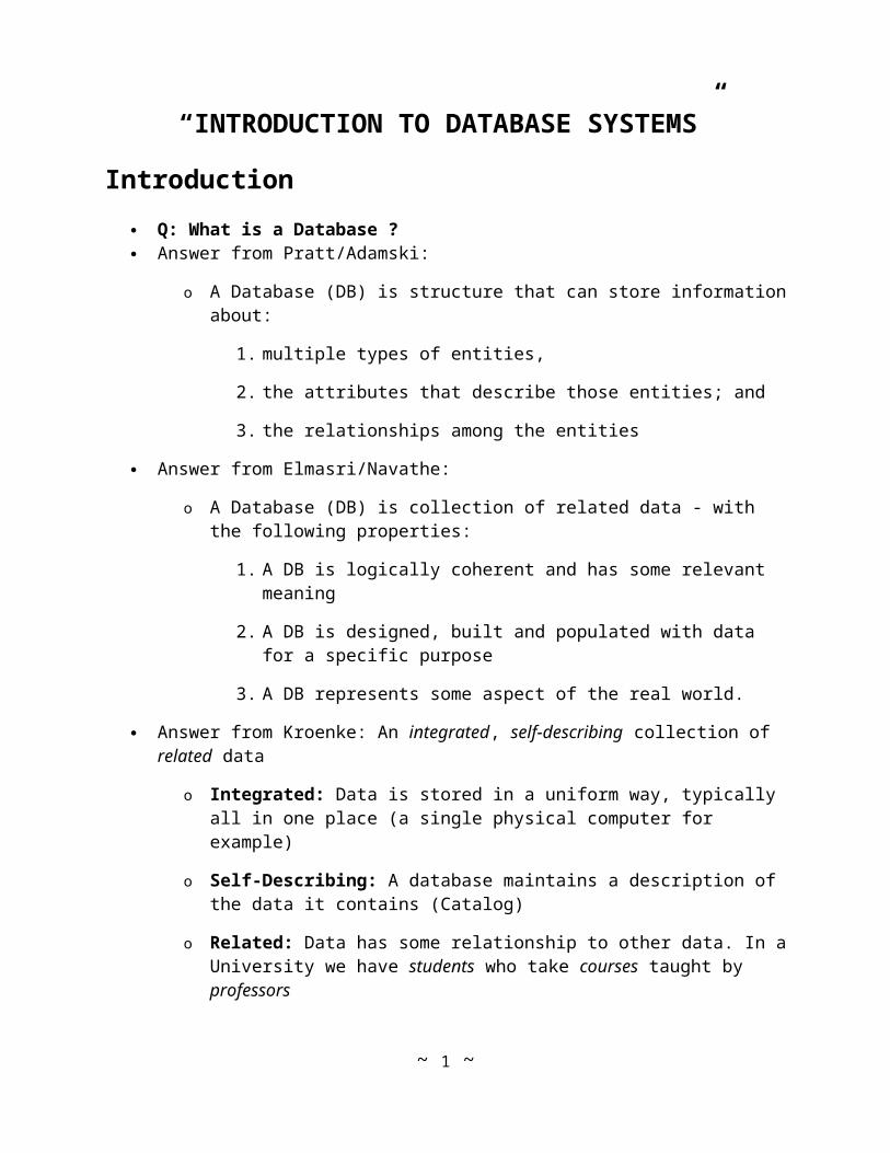
Database Management System (DBMS)A collection of software programs that are used to define, construct, maintain and manipulate data in a database.
Database System (DBS) contains:The Database +The DBMS + Application Programs (what users interact with)
File Systems
File System: A collection of individual files accessed by applications programs Limitations of a File System:
o Separated and Isolated Data - Makes coordinating, assimilating and representing data difficult
o Data Duplication - Wastes space and can lead to data integrity (inconsistency) problems
o Application Program Dependencies - Changes to a single file can require changes to numerous application programs
o Incompatible Files
~ 2 ~
o Lack of Data Sharing - Difficult to control access to files, especially to individual portions of files
Advantages of a DBMS A DBMS can provide:
o Data Consistency and Integrity - by controlling access and minimizing data duplication
o Application program independence - by storing data in a uniform fashion
o Data Sharing - by controlling access to data items, many users can access data concurrently
o Backup and Recovery
o Security and Privacy
o Multiple views of data
Example Database
An Example Database
CustomerID Name Address City State Acct_Number Balance
123 Mr. Smith 123 Lexington Smithville KY 9987 4000
123 Mr. Smith 123 Lexington Smithville KY 9980 2000
124 Mrs. Jones 12 Davis Ave. Smithville KY 8811 1000
125 Mr. Axe 443 Grinder Ln.
Broadville GA 4422 6000
125 Mr. Axe 443 Grinder Ln.
Broadville GA 4433 9000
127 Mr. & Mrs. Builder
661 Parker Rd. Streetville GA 3322 500
127 Mr. & Mrs. Builder
661 Parker Rd. Streetville GA 1122 800
What happens when a customer moves to a new house ? Who should have access to what data in this database ?
What happens if Mr. and Mrs. Builder both try and withdraw $500 from account 3322 ?
~ 3 ~

What happens if the system crashes just as Mr. Axe is depositing his latest paycheck ?
What data is the customer concerned with ?What data is a bank manager concerned with ?
Send a mailing to all customers with checking accounts having greater than $2000 balance
Let all GA customers know of a new branch location
Brief History of Database Systems
1940's, 50's Initial use of computers as calculators. Limited data, focus on algorithms. Science, military applications.
1960's Business uses. Organizational data, customer data, sales, inventory, accounting, etc. File system based, high emphasis on applications programs to extract and assimilate data. Larger amounts of data, relatively simple calculations.
1970's The relational model. Data separated into individual tables. Related by keys. Initially required heavy system resources. Examples: Oracle, Sybase, Informix, Digital RDB, IBM DB2.
1980's Microcomputers - the IBM PC, Apple Macintosh. Database program such as DBase (sort of), Paradox, FoxPro, MS Access. Individual user can crate, maintain small databases.
Late- 1980's Local area networks. Workgroups sharing resources such as files, printers, e-mail. Client/Server Database resides on a central server, applications programs run on client PCs attached to the server over a LAN.
1990's Internet and World Wide Web make databases of all kinds available from a single type of client - the Web Browser. Data warehousing and Data Mining also emerge.
Other types of Databases:
o Object-Oriented Database Systems. Objects (data and methods) stored persistently.
o Distributed Database Systems. Copies of data reside at different locations for redundancy or for performance reasons.
Appropriate Use for a Database
In addition to the advantages already mentioned: o Performance
o Expendability, Flexibility, Scalability
~ 4 ~

o Reduced application development times
o Standards enforcement
However, keep in mind:
o DBMS has High initial cost (although falling)
o DBMS has High Overhead - requires powerful computers
o DBMS are not special purpose software programs
e.g., contrast a canned accouting software package like Quicken or QuickBooks with DBMS like MS Access.
When is a DBMS Not Appropriate? o Database is small with a simple structure
o Applications are simple, special purpose and relatively static.
o Applications have real-time requirementsExamples: Traffic signal controlECU patient monitoring
o Concurrent, multi-user access to data is not required.
Contents of a Database
A Database contains: User Data Metadata
Indexes
Application metadata
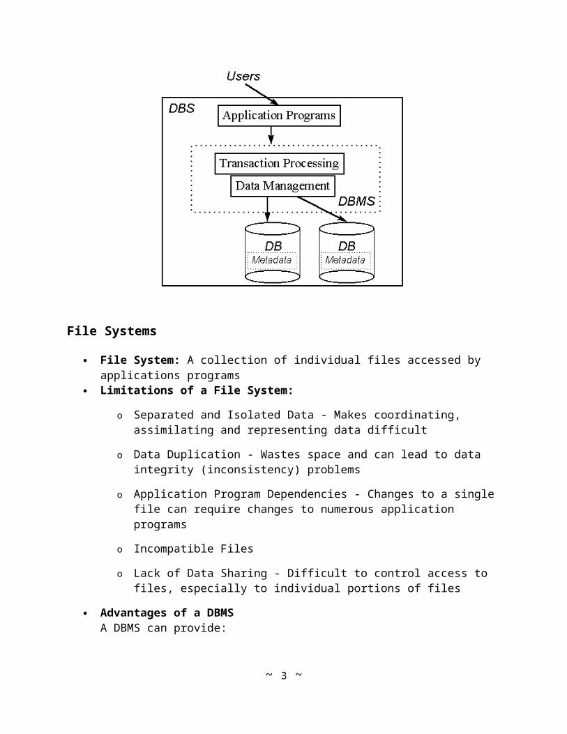
User Data
Data users work with directly by entering, updating and viewing. For our purposes, data will be generally stored in tables with some relationships between
tables.
Each table has one or more columns. A set of columns forms a database record.
Recall our example database for the bank. What were some problems we discussed ?
Here is one improvement - split into 2 tables:
~ 5 ~

Customer Table
CustomerID Name Address City State
123 Mr. Smith 123 Lexington Smithville KY
124 Mrs. Jones 12 Davis Ave. Smithville KY
125 Mr. Axe 443 Grinder Ln. Broadville GA
127 Mr. & Mrs. Builder 661 Parker Rd. Streetville GA
Accounts Table
CustomerID Acct_Number Balance
123 9987 4000
123 9980 2000
124 8811 1000
125 4422 6000
125 4433 9000
127 3322 500
127 1122 800
The customer table has 4 records and 5 columns. The Accounts table has 7 records and 3 columns.
Note relationship between the two tables - CustomerID column.
How should we split data into the tables ? What are the relationships between the tables ?
There are questions that are answered by Database Modeling and Database Design.
Metadata
Recall that a database is self describing Metadata: Data about data.
Data that describe how user data are stored in terms of table name, column name, data type, length, primary keys, etc.
Metadata are typically stored in System tables or System Catalog and are typically only directly accessible by the DBMS or by the system administrator.
Have a look at the Database Documentor feature of MS Access (under the tools menu, choose Analyze and then Documentor). This tool queries the system tables to give all kinds of Metadata for tables, etc. in an MS Access database.
~ 6 ~
Indexes
In keeping with our desire to provide users with several different views of data, indexes provide an alternate means of accessing user data. Sorting and Searching:
An index for our new banking example might include the account numbers in a sorted order.
Indexes allow the database to access a record without having to search through the entire table.
Updating data requires an extra step: The index must also be updated.
Example: Index in a book consists of two things:1) A Keyword stored in order2) A pointer to the rest of the information. In the case of the book, the pointer is a page number.
Applications Metadata
Many DBMS have storage facilities for forms, reports, queries and other application components.
Applications Metadata is accessed via the database development programs.
Example: Look at the Documentor tool in MS Access. It can also show metadata for Queries, Forms, Reports, etc.
Data Modeling and Database Design
Database Design: The activity of specifying the schema of a database in a given data model
Database Schema: The structure of a database that:
o Captures data types, relationships and constraints in data
o Is independent of any application program
o Changes infrequently
Data Model:
o A set of primitives for defining the structure of a database.
o A set of operations for specifying retrieval and updates on a database
o Examples: Relational, Hierarchical, Networked, Object-Oriented
In this course, we focus on the Relational data model.
Database Instance or State: The actual data contained in a database at a given time.
~ 7 ~

The Database Development Process
Two overall approaches: 1. Top-Down: Design systems from an overall organization perspective 2. Bottom-Up: Design systems from a specific perspective - one system at a time.
The following is a very brief outline describing the database development process.
User needs assessment and requirements gathering: Determine what the user's are looking for, what functions should be supported, how the system should behave.
Data Modeling: Based on user requirements, form a logical model of the system. This logical model is then converted to a physical data model (tables, columns, relationships, etc.) that will be implemented.
Implementation: Based on the data model, a database can be created. Applications are then written to perform the required functions.
Testing: The system is tested using real data.
Deployment: The system is deployed to users. Maintenance of the system begins.
There are many variations to this basic development process. A Systems Analysis and Design course (such as CIS 3900 for undergraduates, CIS 9490 for graduates) covers these topics in greater detail.
Designing A Database - A Brief Example
For our Bank example, lets assume that the managers are interested in creating a database to track their customers and accounts.
TablesCUSTOMERSCustomer_Id, Name, Street, City, State, Zip
ACCOUNTSCustomer_Id, Account_Number, Account_Type, Date_Opened, Balance
Note that we use an artificial identifier (a number we make up) for the customer called Customer_Id. Given a Customer_Id, we can uniquely identify the remaining information. We call Customer_Id a Key for the CUSTOMERS table.
o Customer_Id is the key for the CUSTOMERS table. o Account_Number is the key for the ACCOUNTS table.
o Customer_Id in the ACCOUNTS table is called a Foreign Key
~ 8 ~

Notice that when naming columns in the tables we always use an underscore character and do not use any other punctuation. even though Access allows you to use spaces, etc. it is not a good idea.
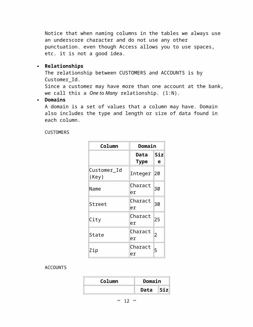
RelationshipsThe relationship between CUSTOMERS and ACCOUNTS is by Customer_Id. Since a customer may have more than one account at the bank, we call this a One to Many relationship. (1:N).
DomainsA domain is a set of values that a column may have. Domain also includes the type and length or size of data found in each column.
CUSTOMERS
Column Domain
Data Type Size
Customer_Id (Key) Integer 20
Name Character 30
Street Character 30
City Character 25
State Character 2
Zip Character 5
ACCOUNTS
Column Domain
Data Type Size
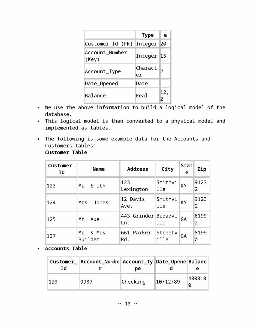
Customer_Id (FK) Integer 20
Account_Number (Key) Integer 15
Account_Type Character 2
Date_Opened Date
Balance Real 12,2
We use the above information to build a logical model of the database. This logical model is then converted to a physical model and implemented as tables.
The following is some example data for the Accounts and Customers tables:Customer Table
Customer_Id Name Address City State Zip
123 Mr. Smith 123 Lexington Smithville KY 91232
~ 9 ~
124 Mrs. Jones 12 Davis Ave. Smithville KY 91232
125 Mr. Axe 443 Grinder Ln. Broadville GA 81992
127 Mr. & Mrs. Builder 661 Parker Rd. Streetville GA 81990
Accounts Table
Customer_Id Account_Number Account_Type Date_Opened Balance
123 9987 Checking 10/12/89 4000.00
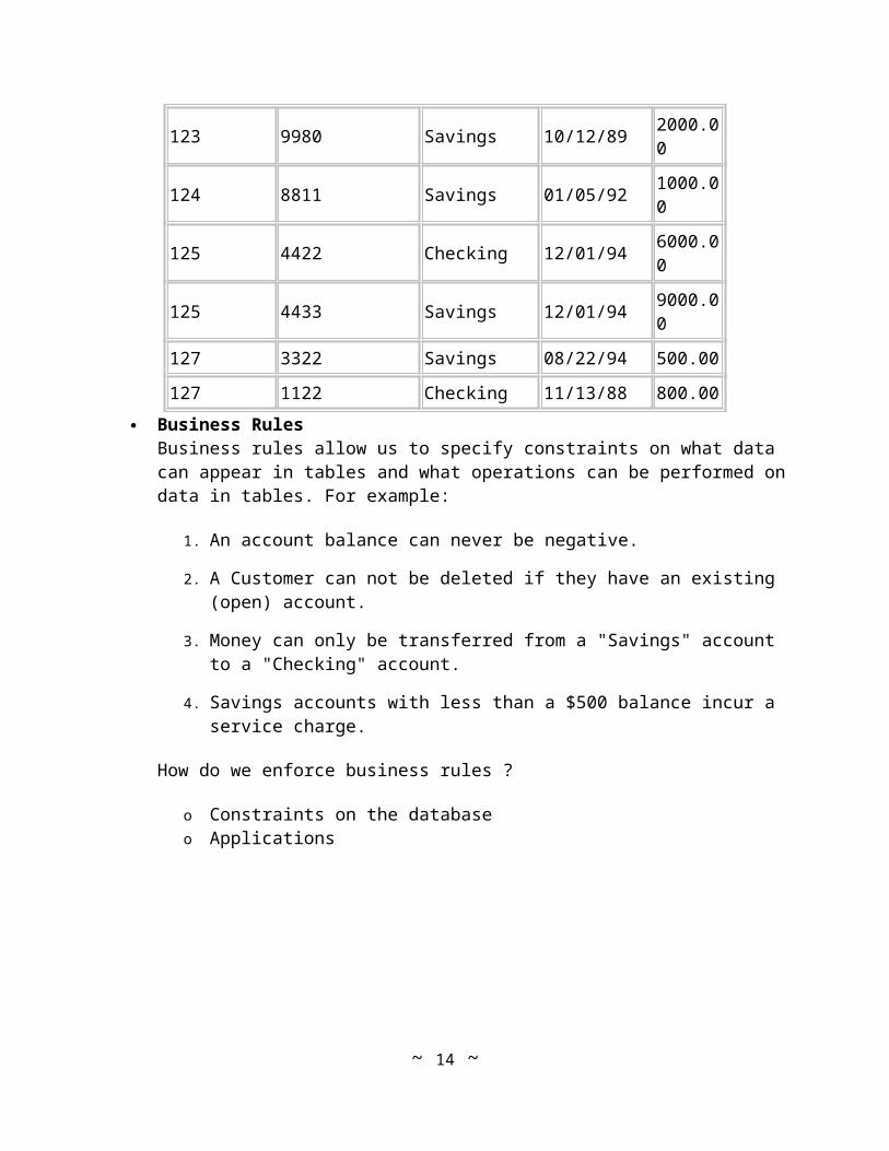
123 9980 Savings 10/12/89 2000.00
124 8811 Savings 01/05/92 1000.00
125 4422 Checking 12/01/94 6000.00
125 4433 Savings 12/01/94 9000.00
127 3322 Savings 08/22/94 500.00
127 1122 Checking 11/13/88 800.00
Business RulesBusiness rules allow us to specify constraints on what data can appear in tables and what operations can be performed on data in tables. For example:
1. An account balance can never be negative.
2. A Customer can not be deleted if they have an existing (open) account.
3. Money can only be transferred from a "Savings" account to a "Checking" account.
4. Savings accounts with less than a $500 balance incur a service charge.
How do we enforce business rules ?
o Constraints on the database o Applications
~ 10 ~

Entity Relationship Modeling
Entity Relationship Modeling: A Set of constructs used to interpret, specify and document logical data requirements for database processing systems.
E-R Models are Conceptual Models of the database. They can not be directly implemented in a database.
Many variations of E-R Modeling used in practice.
Mainly differences in notation, symbols used to represent the 4 main constructs.
E-R Modeling Constructs
E-R Modeling Constructs are: Entity, Relationship, Attributes, Identifiers It is important to get used to this terminology and to be able to use it at the appropriate
time. For example, in the ER Model, we do not refer to tables. Here we call them entities.
Entity: Some identifiable object relevant to the system being built. Examples of Entities are:EMPLOYEECUSTOMERORGANIZATIONPARTINGREDIENTPURCHASE ORDERCUSTOMER ORDERPRODUCT
An instance of an entity is like a specific example:Bill Gates is an Employee of MicrosoftSPAM is a ProductGreenpeace is an OrganizationFlour is an ingredient
Attribute: A characteristic of an Entity. Properties used to distinguish one entity instance from another. Attributes of entity EMPLOYEE might include:EmployeeIDSocial Security NumberFirst NameLast NameStreet AddressCityState
~ 11 ~
ZipCodeDate Hired Health Benefits Plan
Attributes of entity PRODUCT might include:ProductIDProduct_DescriptionWeightSizeCost
Exercise: Come up with a list of attributes for each of the entities above.
Identifier: A special attribute used to identify a specific instance of an entity.o Typically we look for unique identifiers:
o Social Security Number uniquely identifies an EMPLOYEE
o CustomerID uniquely identifies a CUSTOMER
o We can also use two attributes to indicate an identifier: ORDER_NUMBER and LINE_ITEM uniquely identify an item on an order.
Exercise: Choose one of your attributes as the identifier for each of the entities above.
Relationship: An association between two entities.o A CUSTOMER places a CUSTOMER ORDER
An EMPLOYEE takes a CUSTOMER ORDERA STUDENT enrolls in a COURSEA COURSE is taught by a FACULTY MEMBER
o Relationships are typically given names.
o A relationship can include one or more entities
o The degree of a relationship is the number of Entities that participate in the relationship.
o Relationships of degree 2 are called binary relationships. Most relationships in databases are binary.
o Relationship Cardinality refers to the number of entity instances involved in the relationship. For example:one CUSTOMER may place many CUSTOMER ORDERSmany STUDENTS may sign up for many CLASSESone EMPLOYEE receives one PAYCHECKone SALESPERSON is assigned one COMPANY_CAR
~ 12 ~
1:N "One to Many"
N:M "Many to Many"
1:1 "One to One"
o Beware of 1:1 relationships. The two entities involved might be coalesced into one. Also called HAS-A relationship.
o Beware of N:M relationships. Typically split these into two 1:N relationships with an intersection entity.
o Participation of instances in a relationship may be mandatory or optional.
o For example,one CUSTOMER may place many CUSTOMER ORDERSone EMPLOYEE must fill out one or more PAY SHEETS
o This is also called "minimal cardinality" or the "optionality" of a relationship.
E-R Diagrams
The most common way to represent the E-R constructs is by using a diagram There are a wide variety of notations for E-R Diagrams. Most of the differences concern
how relationships are specified and how attributes are shown.
In almost all variations, entities are depicted as rectangles with either pointed or rounded corners. The entity name appears inside.
Relationships can be displayed as diamonds (see below) or can be simply line segments between two entities.
For Relationships, need to convey: Relationship name, degree, cardinality, optionality (minimal cardinality)
Here we will give examples from 4 variations: The Kroenke textbook, Elmasri/Navathe textbook, Oracle Designer/2000 and Visible Analyst.
Variation One - What the Kroenke book uses
Relationship Name: Displayed just outside of the relationship diamond. Degree: Shown by line segments between the relationship diamond and 2 or more
entities.
Cardinality: Displayed inside the relationship diamond.
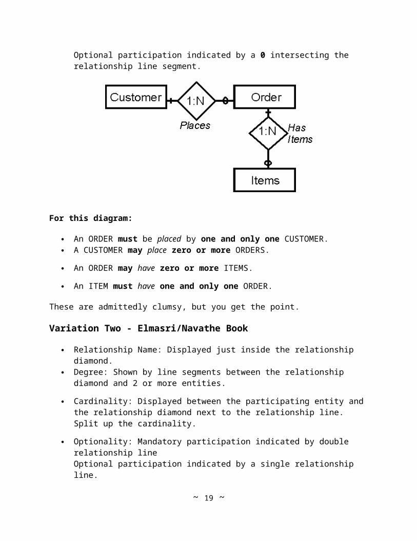
Optionality: Mandatory participation indicated by an intersecting hash mark made perpendicular to the relationship line segment.Optional participation indicated by a 0 intersecting the relationship line segment.
~ 13 ~
For this diagram:
An ORDER must be placed by one and only one CUSTOMER. A CUSTOMER may place zero or more ORDERS.
An ORDER may have zero or more ITEMS.
An ITEM must have one and only one ORDER.
These are admittedly clumsy, but you get the point.
Variation Two - Elmasri/Navathe Book
Relationship Name: Displayed just inside the relationship diamond. Degree: Shown by line segments between the relationship diamond and 2 or more
entities.
Cardinality: Displayed between the participating entity and the relationship diamond next to the relationship line. Split up the cardinality.
Optionality: Mandatory participation indicated by double relationship lineOptional participation indicated by a single relationship line.
~ 14 ~
Variation Three - Oracle Designer/2000 CASE
In Oracle Corporation's Designer/2000, relationships are expressed in a rigid sentence format. For example: An ORDER must be placed by one and only one CUSTOMER.The "be" is mandatory making the verb difficult to get right.
Relationship diamonds are not used.
Relationship Names: Are expressed as a verb phrase starting with "be". There are two phrases, one for each direction of the relationship.This phrase is then written along the line segments for the relationship.
Degree: Shown by line segments between any two entities. As such, 3 way relationships as described in the Kronke book can not exist.
Cardinality: Single participation ("1" in the previous example) is indicated by a single line segment.Multiple participation ("N") is indicated by crow's feet
Optionality: Mandatory participation is indicated by a solid relationship line segment.Optional participation is indicated by a dotted line segment.
~ 15 ~
One ORDER must be placed by one and only one CUSTOMER. One CUSTOMER may be placing zero or more ORDERS.
One ORDER may be made up of zero or more ITEMS.
One ITEM must be an item on one and only one ORDER.
There are a set of tools that can print these "relationship sentences".
Variation Four - Visible Analyst
Visible Analyst Workbench (VAW) uses the rounded box to show an Attributive Entity - one that depends on the existence of a fundamental entity (noted by just the rectangle).
The relationships use the following symbols:
o For cardinality, the crow's feet are used to show a "Many" side of a relationship.
o A single line show a "One" side of the relationship.
~ 16 ~

o Optional participation is shown with an open circle. Thus in the above diagram, a Customer May place one or more Orders.
o Mandatory participation is shown with two hash marks. Thus in the above diagram, an Order Must be placed by one and only one Customer.
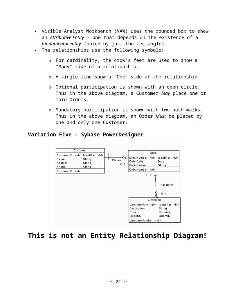
Variation Five - Sybase PowerDesigner
This is not an Entity Relationship Diagram!
It is true: The "Relationships" screen in MS Access is NOT an Entity Relationship diagramming tool. This is a "physical" level diagram of how the tables are actually created.
~ 17 ~
Displaying Attributes
Technically, an Entity-Relationship diagram should show only entities and their relationships.
Consider: Entity-Relationship-Attribute (ERA) model.
Two main ways to display attributes associated with an entity.
1. Attributes appear in ovals attached to the entity. Gets messy.
2. List attributes inside of the entity box.
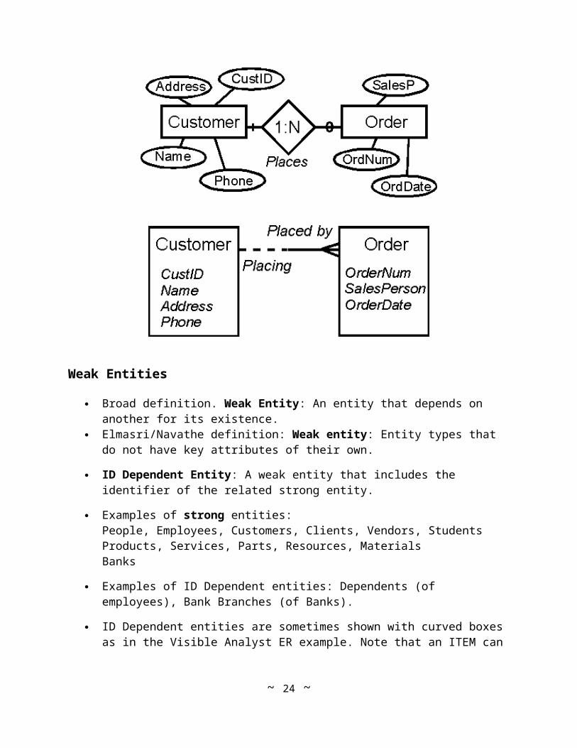
Weak Entities
Broad definition. Weak Entity: An entity that depends on another for its existence. Elmasri/Navathe definition: Weak entity: Entity types that do not have key attributes of
their own.
ID Dependent Entity: A weak entity that includes the identifier of the related strong entity.
Examples of strong entities:People, Employees, Customers, Clients, Vendors, Students Products, Services, Parts, Resources, MaterialsBanks
~ 18 ~
Examples of ID Dependent entities: Dependents (of employees), Bank Branches (of Banks).
ID Dependent entities are sometimes shown with curved boxes as in the Visible Analyst ER example. Note that an ITEM can not exist by itself. It must be identified with a specific Order.
The Elmasri/Navathe notation shows the ID Dependent entity with a double box. The "identifying relationship" (from the strong entity to the weak entity) is shown with a double diamond.
Final note: ID Dependent entities will always result in relations (and later on tables) with composite keys.
Subtype Entities
Attributes of two or more Entities may overlap significantly but not completely. Consider:
Phone Call (Source#, Destination#, Time of day, Duration)LongDistance Call (Source#, Destination#, Time of day, Duration, Long distance Carrier)Cell Phone Call (Source#, Destination#, Time of day, LandTime, AirTime)
One approach would be to put all of the attributes into a single entity.
~ 19 ~

Second approach, put common attributes into a parent or supertype entity and then have 3 subtype entities.
Relationship is called an IS-A relationship.
The above diagram uses the Oracle Designer/2000 symbols for Supertype/Subtype. Below is the same diagram drawn using E-R symbols from the Elmasri/Navathe book.
~ 20 ~

The d in the circle indicates the subtype entity is distinct. Only one subtype entity can participate in an instance.
As before, the double line between the Call entity and the d in the circle indicates the relationship is mandatory.
The Relational Model
Recall, the Relational Model consists of the elements: relations, which are made up of attributes.
A relation is a set of columns (attributes) with values for each attribute such that:
1. Each column (attribute) value must be a single value only.
2. All values for a given column (attribute) must be of the same type.
3. Each column (attribute) name must be unique.
4. The order of columns is insignificant
5. No two rows (tuples) in a relation can be identical.
6. The order of the rows (tuples) is insignificant.
From our discussion of E-R Modelling, we know that an Entity typically corresponds to a relation and that the Entity's attributes become attributes of the relation.
We also discussed how, depending on the relationships between entities, copies of attributes (the identifiers) were placed in related relations.
The process we are following is:
1. Gather user/business requirements. 2. Develop the E-R Model (shown as an E-R Diagram) based on the user/business
requirements.
3. Convert the E-R Model to a set of relations in the relational model
4. Normalize the relations to remove any anomalies (***).
5. Implement the database by creating a table for each normalized relation.
Functional Dependencies
A Functional Dependency describes a relationship between attributes in a single relation. An attribute is functionally dependant on another if we can use the value of one attribute
to determine the value of another.
~ 21 ~
Example: Employee_Name is functionally dependant on Social_Security_Number because Social_Security_Number can be used to determine the value of Employee_Name.
We use the symbol -> to indicate a functional dependency.-> is read functionally determines
Student_ID -> Student_Major Student_ID, Course#, Semester# -> Grade SKU -> Compact_Disk_Title, Artist Model, Options, Tax -> Car_Price Course_Number, Section -> Professor, Classroom, Number of Students
The attributes listed on the left hand side of the -> are called determinants.One can read A -> B as, "A determines B".
Keys and Uniqueness
Key: One or more attributes that uniquely identify a tuple (row) in a relation. The selection of keys will depend on the particular application being considered.
Users can offer some guidance as to what would make an appropriate key. Also this is pretty much an art as opposed to an exact science.
Recall that no two relations should have exactly the same values, thus a candidate key would consist of all of the attributes in a relation.
A key functionally determines a tuple (row).
Not all determinants are keys.
Modification Anomalies
Once our E-R model has been converted into relations, we may find that some relations are not properly specified. There can be a number of problems:
o Deletion Anomaly: Deleting a relation results in some related information (from another entity) being lost.
o Insertion Anomaly: Inserting a relation requires we have information from two or more entities - this situation might not be feasible.
~ 22 ~

Here is a quick example: A company has a Purchase order form:
Our dutiful consultant creates the E-R Model:
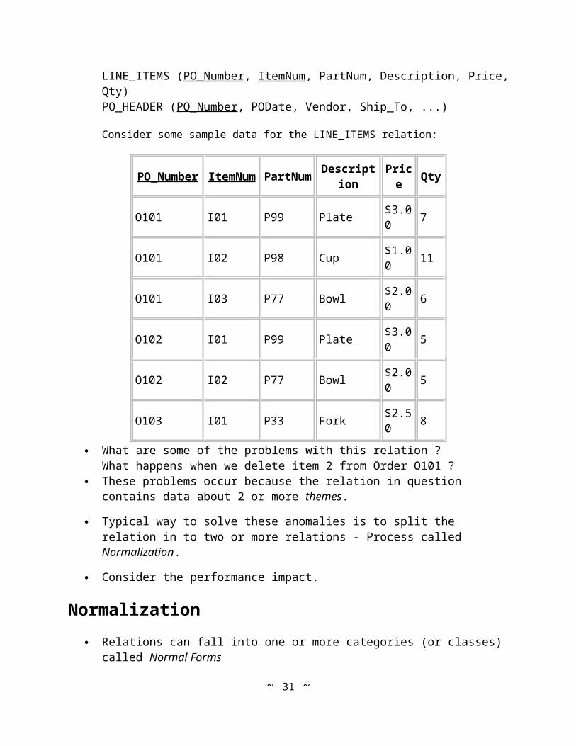
LINE_ITEMS (PO_Number, ItemNum, PartNum, Description, Price, Qty)PO_HEADER (PO_Number, PODate, Vendor, Ship_To, ...)
Consider some sample data for the LINE_ITEMS relation:
~ 23 ~
PO_Number ItemNum PartNum Description Price Qty
O101 I01 P99 Plate $3.00 7
O101 I02 P98 Cup $1.00 11
O101 I03 P77 Bowl $2.00 6
O102 I01 P99 Plate $3.00 5
O102 I02 P77 Bowl $2.00 5
O103 I01 P33 Fork $2.50 8
What are some of the problems with this relation ?What happens when we delete item 2 from Order O101 ?
These problems occur because the relation in question contains data about 2 or more themes.
Typical way to solve these anomalies is to split the relation in to two or more relations - Process called Normalization.
Consider the performance impact.
Normalization
Relations can fall into one or more categories (or classes) called Normal Forms Normal Form: A class of relations free from a certain set of modification anomalies.
Normal forms are given name such as:
o First normal form (1NF)
o Second normal form (2NF)
o Third normal form (3NF)
o Boyce-Codd normal form (BCNF)
o Fourth normal form (4NF)
o Fifth normal form (5NF)
o Domain-Key normal form (DK/NF)
These forms are cumulative. A relation in Third normal form is also in 2NF and 1NF.
First Normal Form (1NF)
A relation is in first normal form if it meets the definition of a relation:
~ 24 ~

1. Each column (attribute) value must be a single value only.
2. All values for a given column (attribute) must be of the same type.
3. Each column (attribute) name must be unique.
4. The order of columns is insignificant.
5. No two rows (tuples) in a relation can be identical.
6. The order of the rows (tuples) is insignificant.
If you have a key defined for the relation, then you can meet the unique row requirement.
Example relation in 1NF:STOCKS (Company, Symbol, Date, Close_Price)
Company Symbol Date Close Price
IBM IBM 01/05/94 101.00
IBM IBM 01/06/94 100.50
IBM IBM 01/07/94 102.00
Netscape NETS 01/05/94 33.00
Netscape NETS 01/06/94 112.00
Second Normal Form (2NF)
A relation is in second normal form (2NF) if all of its non-key attributes are dependent on all of the key.
Relations that have a single attribute for a key are automatically in 2NF.
This is one reason why we often use artificial identifiers as keys.
In the example below, Close Price is dependent on Company, Date and Symbol, Date
The following example relation is not in 2NF:STOCKS (Company, Symbol, Headquarters, Date, Close_Price)
Company Symbol Headquarters Date Close Price
IBM IBM Armonk, NY 01/05/94 101.00
IBM IBM Armonk, NY 01/06/94 100.50
IBM IBM Armonk, NY 01/07/94 102.00
Netscape NETS Sunyvale, CA 01/05/94 33.00
~ 25 ~

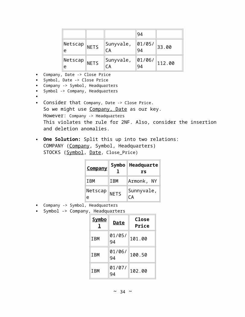
Netscape NETS Sunyvale, CA 01/06/94 112.00 Company, Date -> Close Price Symbol, Date -> Close Price Company -> Symbol, Headquarters Symbol -> Company, Headquarters Consider that Company, Date -> Close Price.
So we might use Company, Date as our key.However: Company -> HeadquartersThis violates the rule for 2NF. Also, consider the insertion and deletion anomalies.
One Solution: Split this up into two relations:COMPANY (Company, Symbol, Headquarters) STOCKS (Symbol, Date, Close_Price)
Company Symbol Headquarters
IBM IBM Armonk, NY
Netscape NETS Sunnyvale, CA Company -> Symbol, Headquarters Symbol -> Company, Headquarters
Symbol Date Close Price
IBM 01/05/94 101.00
IBM 01/06/94 100.50
IBM 01/07/94 102.00
NETS 01/05/94 33.00
NETS 01/06/94 112.00 Symbol, Date -> Close Price
Third Normal Form (3NF)
A relation is in third normal form (3NF) if it is in second normal form and it contains no transitive dependencies.
Consider relation R containing attributes A, B and C.If A -> B and B -> C then A -> C
Transitive Dependency: Three attributes with the above dependencies.
Example: At CUNY:
~ 26 ~

Course_Code -> Course_Num, Section Course_Num, Section -> Classroom, Professor
Example: At Rutgers:
Course_Index_Num -> Course_Num, Section Course_Num, Section -> Classroom, Professor Example:
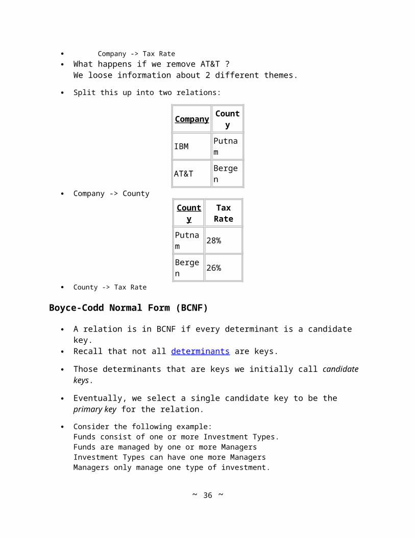
Company County Tax Rate
IBM Putnam 28%
AT&T Bergen 26% Company -> County and County -> Tax Rate thus Company -> Tax Rate
What happens if we remove AT&T ?We loose information about 2 different themes.
Split this up into two relations:
Company County
IBM Putnam
AT&T Bergen
Company -> County
County Tax Rate
Putnam 28%
Bergen 26% County -> Tax Rate
Boyce-Codd Normal Form (BCNF)
A relation is in BCNF if every determinant is a candidate key. Recall that not all determinants are keys.
Those determinants that are keys we initially call candidate keys.
Eventually, we select a single candidate key to be the primary key for the relation.
Consider the following example:Funds consist of one or more Investment Types.Funds are managed by one or more ManagersInvestment Types can have one more ManagersManagers only manage one type of investment.
~ 27 ~

FundID InvestmentType Manager
99 Common Stock Smith
99 Municipal Bonds Jones
33 Common Stock Green
22 Growth Stocks Brown
11 Common Stock Smith FundID, InvestmentType -> Manager FundID, Manager -> InvestmentType Manager -> InvestmentType
In this case, the combination FundID and InvestmentType form a candidate key because we can use FundID,InvestmentType to uniquely identify a tuple in the relation.
Similarly, the combination FundID and Manager also form a candidate key because we can use FundID, Manager to uniquely identify a tuple.
Manager by itself is not a candidate key because we cannot use Manager alone to uniquely identify a tuple in the relation.
Is this relation R(FundID, InvestmentType, Manager) in 1NF, 2NF or 3NF ?Given we pick FundID, InvestmentType as the Primary Key: 1NF for sure.2NF because all of the non-key attributes (Manager) is dependant on all of the key.3NF because there are no transitive dependencies.
Consider what happens if we delete the tuple with FundID 22. We loose the fact that Brown manages the InvestmentType "Growth Stocks."
The following are steps to normalize a relation into BCNF:
1. List all of the determinants.
2. See if each determinant can act as a key (candidate keys).
3. For any determinant that is not a candidate key, create a new relation from the functional dependency. Retain the determinant in the original relation.
For our example:Rorig(FundID, InvestmentType, Manager)
1. The determinants are:FundID, InvestmentTypeFundID, Manager
Manager
2. Which determinants can act as keys ?FundID, InvestmentType YESFundID, Manager YESManager NO
~ 28 ~

3. Create a new relation from the functional dependency:
Rnew(Manager, InvestmentType)Rorig(FundID, Manager)
In this last step, we have retained the determinant "Manager" in the original relation Rorig.
Fourth Normal Form (4NF)
A relation is in fourth normal form if it is in BCNF and it contains no multivalued dependencies.
Multivalued Dependency: A type of functional dependency where the determinant can determine more than one value.
More formally, there are 3 criteria:
1. There must be at least 3 attributes in the relation. call them A, B, and C, for example.
2. Given A, one can determine multiple values of B.Given A, one can determine multiple values of C.
3. B and C are independent of one another.
Book example: Student has one or more majors.Student participates in one or more activities.
StudentID Major Activities
100 CIS Baseball
100 CIS Volleyball
100 Accounting Baseball
100 Accounting Volleyball
200 Marketing Swimming StudentID ->-> Major StudentID ->-> Activities
Portfolio ID Stock Fund Bond Fund
999 Janus Fund Municipal Bonds
999 Janus Fund Dreyfus Short-Intermediate Municipal Bond Fund
999 Scudder Global Fund Municipal Bonds
999 Scudder Global Fund Dreyfus Short-Intermediate Municipal Bond Fund
~ 29 ~

888 Kaufmann Fund T. Rowe Price Emerging Markets Bond Fund
A few characteristics: 1. No regular functional dependencies
2. All three attributes taken together form the key.
3. Latter two attributes are independent of one another.
4. Insertion anomaly: Cannot add a stock fund without adding a bond fund (NULL Value). Must always maintain the combinations to preserve the meaning.
Stock Fund and Bond Fund form a multivalued dependency on Portfolio ID.
PortfolioID ->-> Stock Fund PortfolioID ->-> Bond Fund Resolution: Split into two tables with the common key:
Portfolio ID Stock Fund
999 Janus Fund
999 Scudder Global Fund
888 Kaufmann Fund
Portfolio ID Bond Fund
999 Municipal Bonds
999 Dreyfus Short-Intermediate Municipal Bond Fund
888 T. Rowe Price Emerging Markets Bond Fund
Fifth Normal Form (5NF)There are certain conditions under which after decomposing a relation, it cannot be reassembled back into its original form.
We don't consider these issues here.
Domain Key Normal Form (DK/NF)
A relation is in DK/NF if every constraint on the relation is a logical consequence of the definition of keys and domains.
Constraint: An rule governing static values of an attribute such that we can determine if this constraint is True or False. Examples:
~ 30 ~
1. Functional Dependencies
2. Multivalued Dependencies
3. Inter-relation rules
4. Intra-relation rules
However: Does Not include time dependent constraints.
Key: Unique identifier of a tuple. Domain: The physical (data type, size, NULL values) and semantic (logical) description
of what values an attribute can hold.
There is no known algorithm for converting a relation directly into DK/NF.
De-Normalization
Consider the following relation:CUSTOMER (CustomerID, Name, Address, City, State, Zip)
This relation is not in DK/NF because it contains a functional dependency not implied by the key.
Zip -> City, State
We can normalize this into DK/NF by splitting the CUSTOMER relation into two:CUSTOMER (CustomerID, Name, Address, Zip)CODES (Zip, City, State)
We may pay a performance penalty - each customer address lookup requires we look in two relations (tables).
In such cases, we may de-normalize the relations to achieve a performance improvement.
All-in-One Example
Many of you asked for a "complete" example that would run through all of the normal forms from beginning to end using the same tables. This is tough to do, but here is an attempt:
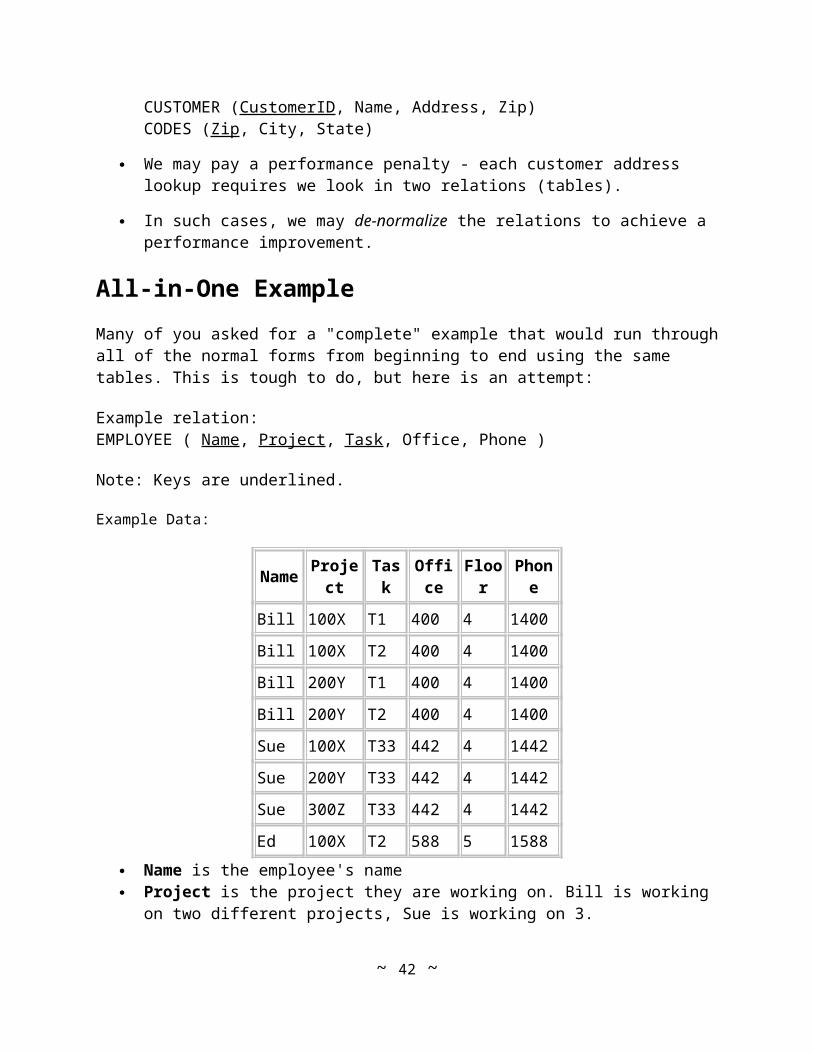
Example relation:EMPLOYEE ( Name, Project, Task, Office, Phone )
Note: Keys are underlined.
Example Data:
Name Project Task Office Floor Phone
~ 31 ~

Bill 100X T1 400 4 1400
Bill 100X T2 400 4 1400
Bill 200Y T1 400 4 1400
Bill 200Y T2 400 4 1400
Sue 100X T33 442 4 1442
Sue 200Y T33 442 4 1442
Sue 300Z T33 442 4 1442
Ed 100X T2 588 5 1588
Name is the employee's name Project is the project they are working on. Bill is working on two different projects, Sue
is working on 3.
Task is the current task being worked on. Bill is now working on Tasks T1 and T2. Note that Tasks are independent of the project. Examples of a task might be faxing a memo or holding a meeting.
Office is the office number for the employee. Bill works in office number 400.
Floor is the floor on which the office is located.
Phone is the phone extension. Note this is associated with the phone in the given office.
First Normal Form
Assume the key is Name, Project, Task. Is EMPLOYEE in 1NF ?
Second Normal Form
List all of the functional dependencies for EMPLOYEE. Are all of the non-key attributes dependant on all of the key ?
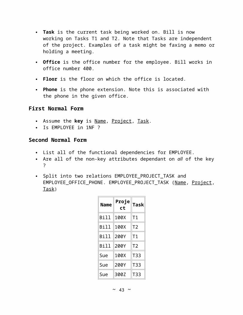
Split into two relations EMPLOYEE_PROJECT_TASK and EMPLOYEE_OFFICE_PHONE. EMPLOYEE_PROJECT_TASK (Name, Project, Task)
Name Project Task
Bill 100X T1
Bill 100X T2
Bill 200Y T1
Bill 200Y T2
~ 32 ~

Sue 100X T33
Sue 200Y T33
Sue 300Z T33
Ed 100X T2
EMPLOYEE_OFFICE_PHONE (Name, Office, Floor, Phone)
Name Office Floor Phone
Bill 400 4 1400
Sue 442 4 1442
Ed 588 5 1588
Third Normal Form
Assume each office has exactly one phone number. Are there any transitive dependencies ?
Where are the modification anomalies in EMPLOYEE_OFFICE_PHONE ?
Split EMPLOYEE_OFFICE_PHONE.
EMPLOYEE_PROJECT_TASK (Name, Project, Task)
Name Project Task
Bill 100X T1
Bill 100X T2
Bill 200Y T1
Bill 200Y T2
Sue 100X T33
Sue 200Y T33
Sue 300Z T33
Ed 100X T2
EMPLOYEE_OFFICE (Name, Office, Floor)
Name Office Floor
Bill 400 4
~ 33 ~
Sue 442 4
Ed 588 5
EMPLOYEE_PHONE (Office, Phone)
Office Phone
400 1400
442 1442
588 1588
Boyce-Codd Normal Form
List all of the functional dependencies for EMPLOYEE_PROJECT_TASK, EMPLOYEE_OFFICE and EMPLOYEE_PHONE. Look at the determinants.
Are all determinants candidate keys ?
Forth Normal Form
Are there any multivalued dependencies ? What are the modification anomalies ?
Split EMPLOYEE_PROJECT_TASK.
EMPLOYEE_PROJECT (Name, Project )
EMPLOYEE_TASK (Name, Task )
Name Task
Bill T1
Bill T2
Sue T33
Ed T2
EMPLOYEE_OFFICE (Name, Office, Floor)
~ 34 ~
Name Project
Bill 100X
Bill 200Y
Sue 100X
Sue 200Y
Sue 300Z
Ed 100X

Name Office Floor
Bill 400 4
Sue 442 4
Ed 588 5
R4 (Office, Phone)
Office Phone
400 1400
442 1442
588 1588
At each step of the process, we did the following:
1. Write out the relation 2. (optionally) Write out some example data.
3. Write out all of the functional dependencies
4. Starting with 1NF, go through each normal form and state why the relation is in the given normal form.
Another short example
Consider the following example of normalization for a CUSTOMER relation.
Relation NameCUSTOMER (CustomerID, Name, Street, City, State, Zip, Phone)
Example Data
CustomerID Name Street City State Zip Phone
C101 Bill Smith 123 First St. New Brunswick NJ 07101 732-555-1212
C102 Mary Green 11 Birch St. Old Bridge NJ 07066 908-555-1212
Functional Dependencies
CustomerID -> Name, Street, City, State, Zip, Phone
~ 35 ~
Zip -> City, State
Normalization
1NF Meets the definition of a relation. 2NF All non key attributes are dependent on all of the key.
3NF There are no transitive dependencies.
BCNF Relation CUSTOMER is not in BCNF because one of the determinants Zip can not act as a key for the entire relation. Solution: Split CUSTOMER into two relations:CUSTOMER (CustomerID, Name, Street, Zip, Phone)ZIPCODES (Zip, City, State)
Check both CUSTOMER and ZIPCODE to ensure they are both in 1NF up to BCNF.
4NF There are no multi-valued dependencies in either CUSTOMER or ZIPCODES.
As a final step, consider de-normalization.
Relational Algebra:
Elmasri/Navathe (3rd) ed.
Kroenke (7th ed.)
Connolly/Begg (3rd Ed.)
Rob/Coronel (5th ed)
Hoffer, Prescott & McFadden
(6th ed.)
Mata-Toledo /
Cushman
Chapter 7 Chapter 8 Chapter 4 N/A N/A Shaum's Outlines Ch. 2
Recall, the Relational Model consists of the elements: relations, which are made up of attributes.
A relation is a set of attributes with values for each attribute such that:
1. Each attribute value must be a single value only (atomic).
2. All values for a given attribute must be of the same type (or domain).
3. Each attribute name must be unique.
4. The order of attributes is insignificant
5. No two rows (tuples) in a relation can be identical.
~ 36 ~

6. The order of the rows (tuples) is insignificant.
Relational Algebra is a collection of operations on Relations.
Relations are operands and the result of an operation is another relation.
Two main collections of relational operators:
1. Set theory operations:Union, Intersection, Difference and Cartesian product.
2. Specific Relational Operations:Selection, Projection, Join, Division
Set Theoretic Operations
Consider the following relations R and S R
First Last Age
Bill Smith 22
Sally Green 28
Mary Keen 23
Tony Jones 32
S
First Last Age
Forrest Gump 36
Sally Green 28
DonJuan DeMarco 27
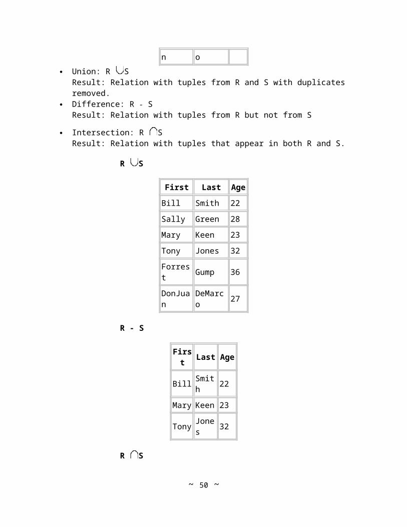
Union: R S Result: Relation with tuples from R and S with duplicates removed.
Difference: R - S Result: Relation with tuples from R but not from S
Intersection: R S Result: Relation with tuples that appear in both R and S.
R S
~ 37 ~

First Last Age
Bill Smith 22
Sally Green 28
Mary Keen 23
Tony Jones 32
Forrest Gump 36
DonJuan DeMarco 27
R - S
First Last Age
Bill Smith 22
Mary Keen 23
Tony Jones 32
R S
First Last Age
Sally Green 28
Union Compatible Relations
Attributes of relations need not be identical to perform union, intersection and difference operations.
However, they must have the same number of attributes or arity and the domains for corresponding attributes must be identical.
Domain is the datatype and size of an attribute.
The degree of relation R is the number of attributes it contains.
Definition: Two relations R and S are union compatible if and only if they have the same degree and the domains of the corresponding attributes are the same.
Some additional properties:
o Union, Intersection and difference operators may only be applied to Union Compatible relations.
~ 38 ~

o Union and Intersection are commutative operationsR S = S RR S = S R
o Difference operation is NOT commutative.R - S not equal S - R
o The resulting relations may not have meaningful names for the attributes. Convention is to use the attribute names from the first relation.
Exercises
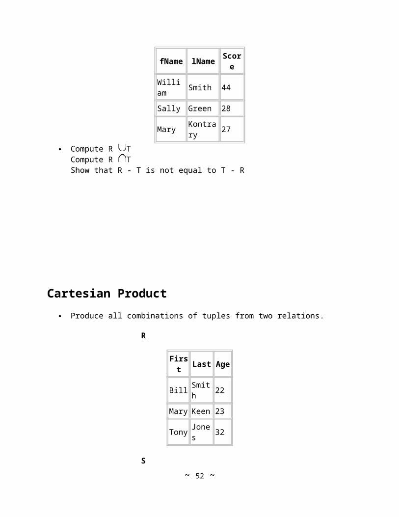
Assume relation T
fName lName Score
William Smith 44
Sally Green 28
Mary Kontrary 27
Compute R TCompute R TShow that R - T is not equal to T - R
Cartesian Product
Produce all combinations of tuples from two relations.
R
First Last Age
Bill Smith 22
Mary Keen 23
Tony Jones 32
~ 39 ~

S
Dinner Dessert
Steak Ice Cream
Lobster Cheesecake
R X S
First Last Age Dinner Dessert
Bill Smith 22 Steak Ice Cream
Bill Smith 22 Lobster Cheesecake
Mary Keen 23 Steak Ice Cream
Mary Keen 23 Lobster Cheesecake
Tony Jones 32 Steak Ice Cream
Tony Jones 32 Lobster Cheesecake
Selection Operator
Selection and Projection are unary operators. The selection operator is sigma:
The selection operation acts like a filter on a relation by returning only a certain number of tuples.
The resulting relation will have the same degree as the original relation.
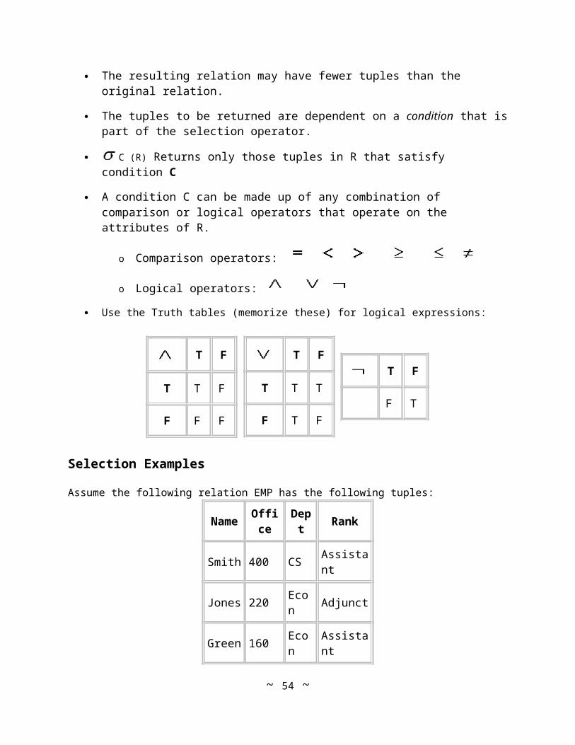
The resulting relation may have fewer tuples than the original relation.
The tuples to be returned are dependent on a condition that is part of the selection operator.
C (R) Returns only those tuples in R that satisfy condition C
A condition C can be made up of any combination of comparison or logical operators that operate on the attributes of R.
o Comparison operators:
o Logical operators:
Use the Truth tables (memorize these) for logical expressions:
~ 40 ~

T F
T T F
F F F
T F
T T T
F T F
T F
F T
Selection Examples
Assume the following relation EMP has the following tuples:
Name Office Dept Rank
Smith 400 CS Assistant
Jones 220 Econ Adjunct
Green 160 Econ Assistant
Brown 420 CS Associate
Smith 500 Fin Associate
Select only those Employees in the CS department:
Dept = 'CS' (EMP)Result:
Name Office Dept Rank
Smith 400 CS Assistant
Brown 420 CS Associate
Select only those Employees with last name Smith who are assistant professors:
Name = 'Smith' Rank = 'Assistant' (EMP)Result:
Name Office Dept Rank
Smith 400 CS Assistant
Select only those Employees who are either Assistant Professors or in the Economics department:
Rank = 'Assistant' Dept = 'Econ' (EMP)Result:
~ 41 ~
Name Office Dept Rank
Smith 400 CS Assistant
Jones 220 Econ Adjunct
Green 160 Econ Assistant
Select only those Employees who are not in the CS department or Adjuncts:
(Rank = 'Adjunct' Dept = 'CS') (EMP)Result:
Name Office Dept Rank
Green 160 Econ Assistant
Smith 500 Fin Associate
Exercises
Evaluate the following expressions:
1. (Rank = 'Adjunct' Dept = 'CS') (EMP)
2. Rank = 'Associate' ( Dept = 'CS' EMP )
3. Dept = 'CS' ( Rank = 'Associate' EMP )
4. Rank = 'Associate' Dept = 'CS' (EMP)
5. Age > 26 (R S)
For this expression, use R and S from the Set Theoretic Operations section above.
Do expressions 2, 3 and 4 above all evaluate ot the same thing?
Projection Operator
Projection is also a Unary operator. The Projection operator is pi:
Projection limits the attributes that will be returned from the original relation.
The general syntax is: attributes RWhere attributes is the list of attributes to be displayed and R is the relation.
~ 42 ~
The resulting relation will have the same number of tuples as the original relation (unless there are duplicate tuples produced).
The degree of the resulting relation may be equal to or less than that of the original relation.
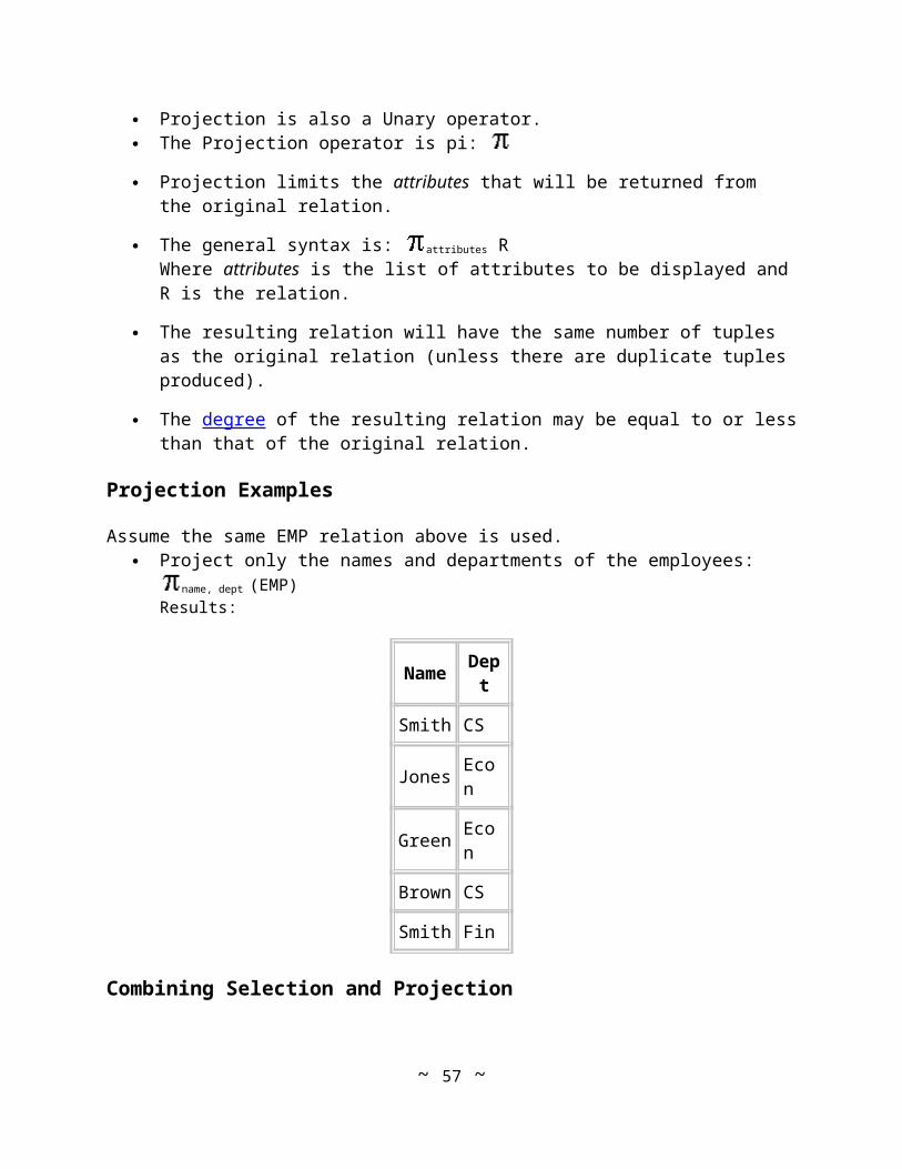
Projection Examples
Assume the same EMP relation above is used. Project only the names and departments of the employees:
name, dept (EMP)Results:
Name Dept
Smith CS
Jones Econ
Green Econ
Brown CS
Smith Fin
Combining Selection and Projection
The selection and projection operators can be combined to perform both operations. Show the names of all employees working in the CS department:
name ( Dept = 'CS' (EMP) )Results:
Name
Smith
Brown
Show the name and rank of those Employees who are not in the CS department or Adjuncts:
name, rank ( (Rank = 'Adjunct' Dept = 'CS') (EMP) )Result:
Name Rank
Green Assistant
~ 43 ~

Smith Associate
Exercises
Evaluate the following expressions:
1. name, rank ( (Rank = 'Adjunct' Dept = 'CS') (EMP) )
2. fname, age ( Age > 22 (R S) )
For this expression, use R and S from the Set Theoretic Operations section above.
3. office > 300 ( name, rank (EMP))
Aggregate Functions
We can also apply Aggregate functions to attributes and tuples:o SUM
o MINIMUM
o MAXIMUM
o AVERAGE, MEAN, MEDIAN
o COUNT
Aggregate functions are sometimes written using the Projection operator or the Script F
character: as in the Elmasri/Navathe book.
Aggregate Function Examples
Assume the relation EMP has the following tuples:
Name Office Dept Salary
Smith 400 CS 45000
Jones 220 Econ 35000
Green 160 Econ 50000
Brown 420 CS 65000
Smith 500 Fin 60000
~ 44 ~

Find the minimum Salary: MIN (salary) (EMP)Results:
MIN(salary)
35000
Find the average Salary: AVG (salary) (EMP)Results:
AVG(salary)
51000
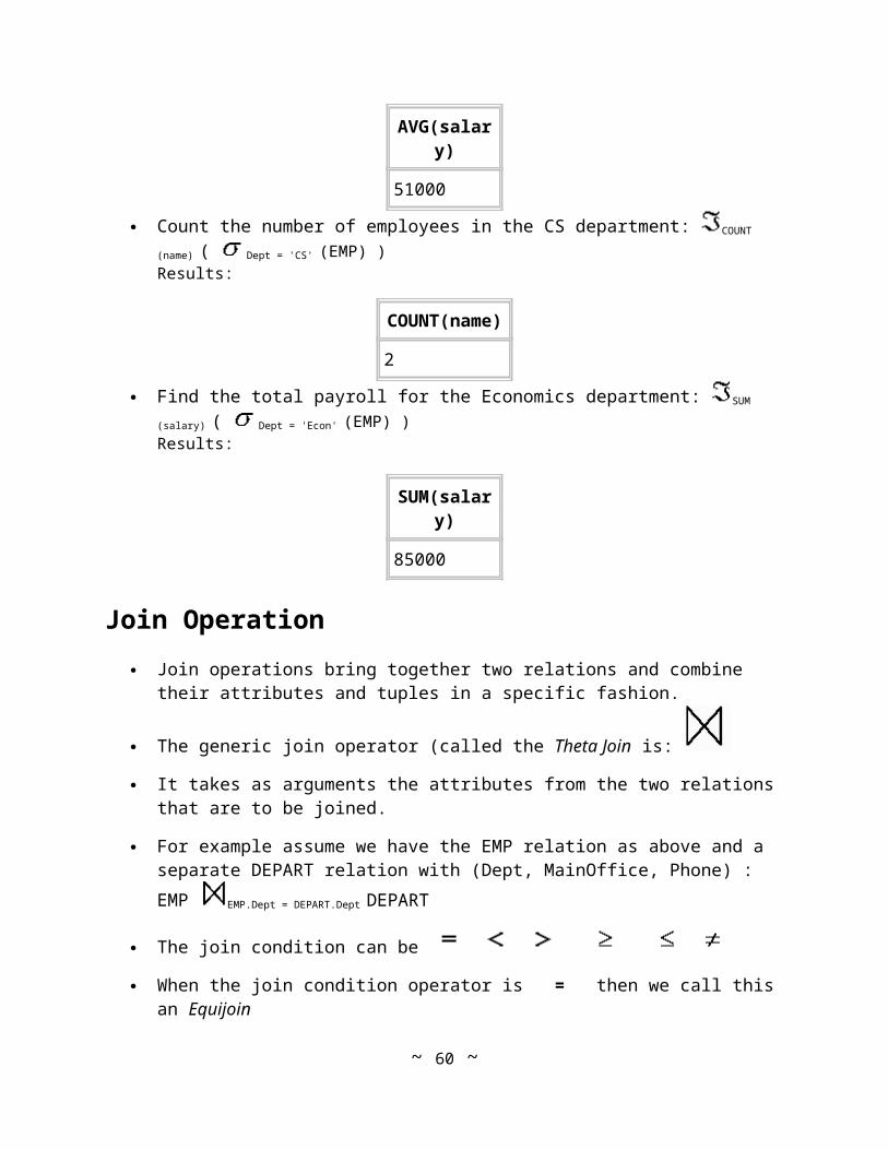
Count the number of employees in the CS department: COUNT (name) ( Dept = 'CS' (EMP) )Results:
COUNT(name)
2
Find the total payroll for the Economics department: SUM (salary) ( Dept = 'Econ' (EMP) )Results:
SUM(salary)
85000
Join Operation
Join operations bring together two relations and combine their attributes and tuples in a specific fashion.
The generic join operator (called the Theta Join is:
It takes as arguments the attributes from the two relations that are to be joined.
For example assume we have the EMP relation as above and a separate DEPART relation with (Dept, MainOffice, Phone) :
EMP EMP.Dept = DEPART.Dept DEPART
The join condition can be
When the join condition operator is = then we call this an Equijoin
Note that the attributes in common are repeated.
~ 45 ~

Join Examples
Assume we have the EMP relation from above and the following DEPART relation:
Dept MainOffice Phone
CS 404 555-1212
Econ 200 555-1234
Fin 501 555-4321
Hist 100 555-9876
Find all information on every employee including their department info:
EMP emp.Dept = depart.Dept DEPARTResults:
Name Office EMP.Dept Salary DEPART.Dept MainOffice Phone
Smith 400 CS 45000 CS 404 555-1212
Jones 220 Econ 35000 Econ 200 555-1234
Green 160 Econ 50000 Econ 200 555-1234
Brown 420 CS 65000 CS 404 555-1212
Smith 500 Fin 60000 Fin 501 555-4321
Find all information on every employee including their department info where the employee works in an office numbered less than the department main office:
EMP (emp.office < depart.mainoffice) (emp.dept = depart.dept) DEPARTResults:
Name Office EMP.Dept Salary DEPART.Dept MainOffice Phone
Smith 400 CS 45000 CS 404 555-1212
Green 160 Econ 50000 Econ 200 555-1234
Smith 500 Fin 60000 Fin 501 555-4321
Natural Join
~ 46 ~

Notice in the generic (Theta) join operation, any attributes in common (such as dept above) are repeated.
The Natural Join operation removes these duplicate attributes.
The natural join operator is: *
We can also assume using * that the join condition will be = on the two attributes in common.
Example: EMP * DEPARTResults:
Name Office Dept Salary MainOffice Phone
Smith 400 CS 45000 404 555-1212
Jones 220 Econ 35000 200 555-1234
Green 160 Econ 50000 200 555-1234
Brown 420 CS 65000 404 555-1212
Smith 500 Fin 60000 501 555-4321
Outer Join
In the Join operations so far, only those tuples from both relations that satisfy the join condition are included in the output relation.
The Outer join includes other tuples as well according to a few rules.
Three types of outer joins:
1. Left Outer Join includes all tuples in the left hand relation and includes only those matching tuples from the right hand relation.
2. Right Outer Join includes all tuples in the right hand relation and includes ony those matching tuples from the left hand relation.
3. Full Outer Join includes all tuples in the left hand relation and from the right hand relation.
Examples: Assume we have two relations: PEOPLE and MENU:
~ 47 ~

PEOPLE:
Name Age Food
Alice 21 Hamburger
Bill 24 Pizza
Carl 23 Beer
Dina 19 Shrimp
MENU:
Food Day
Pizza Monday
Hamburger Tuesday
Chicken Wednesday
Pasta Thursday
Tacos Friday
PEOPLE people.food = menu.food MENU
Name Age people.Food menu.Food Day
Alice 21 Hamburger Hamburger Tuesday
Bill 24 Pizza Pizza Monday
Carl 23 Beer NULL NULL
Dina 19 Shrimp NULL NULL
PEOPLE people.food = menu.food MENU
Name Age people.Food menu.Food Day
Bill 24 Pizza Pizza Monday
Alice 21 Hamburger Hamburger Tuesday
NULL NULL NULL Chicken Wednesday
NULL NULL NULL Pasta Thursday
NULL NULL NULL Tacos Friday
PEOPLE people.food = menu.food MENU
~ 48 ~

Name Age people.Food menu.Food Day
Alice 21 Hamburger Hamburger Tuesday
Bill 24 Pizza Pizza Monday
Carl 23 Beer NULL NULL
Dina 19 Shrimp NULL NULL
NULL NULL NULL Chicken Wednesday
NULL NULL NULL Pasta Thursday
NULL NULL NULL Tacos Friday
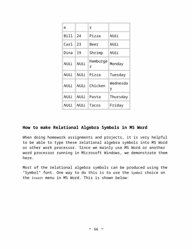
Outer Union
The Outer Union operation is applied to partially union compatible relations. Operator is: *
Example: PEOPLE * MENU
Name Age Food Day
Alice 21 Hamburger NULL
Bill 24 Pizza NULL
Carl 23 Beer NULL
Dina 19 Shrimp NULL
NULL NULL Hamburger Monday
NULL NULL Pizza Tuesday
NULL NULL Chicken Wednesday
NULL NULL Pasta Thursday
NULL NULL Tacos Friday
How to make Relational Algebra Symbols in MS Word
~ 49 ~
When doing homework assignments and projects, it is very helpful to be able to type these relational algebra symbols into MS Word or other work processor. Since we mainly use MS Word or another word processor running in Microsoft Windows, we demonstrate them here.
Most of the relational algebra symbols can be produced using the "Symbol" font. One way to do this is to use the Symbol choice on the Insert menu in MS Word. This is shown below:
The following dialog box will appear:
By default, the symbols displayed on this screen will use the Symbol font.
Some symbols such as join and outer join are not available in this fashion. For these you can copy and paste the graphics in the MS Word file linked here. All of the relational algebra symbols are included.
Structured Query Language
~ 50 ~
SQL was first implemented in IBM's System R in the late 1970's. SQL is the de-facto standard query language for creating and manipulating data in
relational databases.
Some minor syntax differences, but the majority of SQL is standard across MS Access, Oracle, Sybase, Informix, etc.
SQL is either specified by a command-line tool or is embedded into a general purpose programming language such as Cobol, "C", Pascal, etc.
SQL is a standardized language monitored by the American National Standards Institute (ANSI) as well as by National Institute of Standards (NIST).
o ANSI 1990 - SQL 1 standard
o ANSI 1992 - SQL 2 Standard (sometimes called SQL-92)
o SQL 3 - adds some Object oriented concepts
SQL has two major parts:
1. Data Definition Language (DDL) Used to create (define) data structures such as tables, indexes, clusters
2. Data Manipulation Language (DML) is used to store, retrieve and update data from tables.
SQL Data Types
Each implementation of SQL uses slightly different names for the data types.
Numeric Data Types
Integers: INTEGER, INT or SMALLINT Real Numbers: FLOAT, REAL, DOUBLE, PRECISION
Formatted Numbers: DECIMAL(i,j), NUMERIC(i,j)
Character Strings
Two main types: Fixed length and variable length. Fixed length of n characters: CHAR(n) or CHARACTER(n)
Variable length up to size n: VARCHAR(n)
Date and Time
Note: Implementations vary widely for these data types.
~ 51 ~
DATE
Has 10 positions in the format: YYYY-MM-DD
TIME Has 8 positions in the format: HH:MM:SS
TIME(i)
Defines the TIME data type with an additional i positions for fractions of a second. For example:HH:MM:SS:dd
Offset from UTZ. +/- HH:MM
TIMESTAMP
INTERVAL
Used to specify some span of time measured in days or minutes, etc.
Other ways of expressing dates:
o Store as characters or integers with Year, Month Day:19972011
o Store as Julian date:1997283
Both MS Access and Oracle store date and time information together in a DATE data type.
Examples of Data Types for Some Popular RDBMS
Data types most often used are shown in Bold letters MS Access Examples from the MS Access Help File (c) Microsoft:
Data Type Storage
Size Range of Values
Byte 1 byte 0 to 255
Boolean 2 bytes True or False.
Integer 2 bytes -32,768 to 32,767.
Long (long integer)
4 bytes -2,147,483,648 to 2,147,483,647.
Single (single-precision floating-point)
4 bytes -3.402823E38 to -1.401298E-45 for negative values; 1.401298E-45 to 3.402823E38 for positive values.
Double (double-precision floating-point)
8 bytes -1.79769313486232E308 to -4.94065645841247E-324 for negative values; 4.94065645841247E-324 to 1.79769313486232E308 for positive values.
Currency (scaled 8 bytes -922,337,203,685,477.5808 to 922,337,203,685,477.5807.
~ 52 ~

integer)
Date 8 bytes January 1, 100 to December 31, 9999.
Object 4 bytes Any Object reference.
String (variable-length)
10 bytes + string length
0 to approx. 2 billion (approx. 65,400 for MS Windows version 3.1).
String (fixed-length)
Length of string
1 to approximately 65,400.
Variant (with numbers)
16 bytes Any numeric value up to the range of a Double.
Variant (with characters)
22 bytes + string length
Same range as for variable-length String.
Oracle supports the following data types:
o Numeric: BINARY_INTEGER, DEC, DECIMAL, DOUBLE PRECISION, FLOAT, INT, INTEGER, NATURAL, NATURALN, NUMBER, NUMERIC, PLS_INTEGER, POSITIVE, POSITIVEN, REAL, SMALLINT
o Date: DATENote: Also stores time.
o Character: CHAR, CHARACTER, STRING, VARCHAR, VARCHAR2
o Others: BOOLEAN, LONG, LONG RAW, RAW
Note: You will not need to memorize the above two tables for exams, etc. They are only there for your reference.
Data Definition Language
DDL is used to define the schema of the database. Create a database schema
Create, Drop or Alter a table
Create or Drop an Index
Define Integrity constraints
Define access privileges to users
Define access privileges on objects
SQL2 specification supports the creation of multiple schemas per database each with a distinct owner and authorized users.
Creating a Schema
~ 53 ~
Note: To try out these SQL examples in MS Access, go to the Queries form and choose New, then choose Design View and then close the next dialog box. Under the View menu, choose SQL. From this point, you can type in any SQL statement and execute it. Note that MS Access's DDL syntax is extremely limited. Most of the DDL statements below (including domains, NOT NULL constraints and referential integrity constraints) are not supported.
Creating a Table: CREATE TABLE employee ( Last_Name VARCHAR(20) NOT NULL, First_name VARCHAR(18) NOT NULL, Soc_Sec VARCHAR(11) NOT NULL, Date_of_Birth DATE, Salary NUMBER(8,2) ) ; CREATE TABLE dependant ( Last_Name VARCHAR(20) NOT NULL, First_name VARCHAR(18) NOT NULL, Soc_Sec VARCHAR(11) NOT NULL, Date_of_Birth DATE, Employee_Soc_Sec VARCHAR(11) NOT NULL ); Note: When naming tables, columns and other database objects, do not include spaces in
the names. For example, do not call the last name column: Last Name If you wish to separate words in a name, use the underscore character.
Specifying Primary and Foreign keys:
CREATE TABLE order_header ( order_number NUMBER(10,0) NOT NULL, order_date DATE, sales_person VARCHAR(25), bill_to VARCHAR(35), bill_to_address VARCHAR(45), bill_to_city VARCHAR(20), bill_to_state VARCHAR(2), bill_to_zip VARCHAR(10), PRIMARY KEY (order_number) ); CREATE TABLE order_items ( order_number NUMBER(10,0) NOT NULL, line_item NUMBER(4,0) NOT NULL, part_number VARCHAR(12) NOT NULL, quantity NUMBER(4,0), PRIMARY KEY (order_number, line_item), FORIEGN KEY (order_number) REFERENCES order_header (order_number), FOREIGN KEY (part_number) REFERENCES parts (part_number) ); CREATE INDEX order_index ON order_header (order_number) ASC ; CREATE INDEX items_index
~ 54 ~

ON order_items (order_number, line_item) ASC ; Example from MS Access: CREATE TABLE employee ( FirstName TEXT, LastName TEXT, ssn INTEGER CONSTRAINT ssnConstraint PRIMARY KEY ); CREATE INDEX employee_index ON employee (ssn) ;
Specifying Constraints on Columns and Tables
Constraints on attributes: o NOT NULL - Attribute may not take a NULL value
o DEFAULT - Store a given default value i no value is specified
o PRIMARY KEY - Indicate which attribute(s) form the primary key
o FOREIGN KEY - Indicate which attribute(s) form a foreign key. This enforces referential integrity
o UNIQUE - Indicates which attribute(s) must have unique values.
Specify when constraint should be enforced:
o Immediate
o Deferrable until commit time
Referential Integrity Constraint: Specify the behavior for child tuples when a parent tuple is modified.
Action to take if referential integrity is violated:
o SET NULL - Child tuples foreign key is set to NULL - Orphans.
o SET DEFAULT - Set the value of the foreign key to some default value.
o CASCADE - Child tuples are updated (or deleted) according to the action take on the parent tuple.
Examples of ON DELETE and ON UPDATE
CREATE TABLE order_items ( order_number NUMBER(10,0) NOT NULL, line_item NUMBER(4,0) NOT NULL, part_number VARCHAR(12) NOT NULL, quantity NUMBER(4,0), PRIMARY KEY (order_number, line_item),
~ 55 ~

FORIEGN KEY (order_number) REFERENCES order_header (order_number) ON DELETE SET DEFAULT ON UPDATE CASCADE, FOREIGN KEY (part_number) REFERENCES parts (part_number) );
Constraints can also be given names so that they can later be modified or dropped easily.
CREATE TABLE order_header ( order_number NUMBER(10,0) NOT NULL, order_date DATE, sales_person VARCHAR(25), bill_to VARCHAR(35), bill_to_address VARCHAR(45), bill_to_city VARCHAR(20), bill_to_state VARCHAR(2), bill_to_zip VARCHAR(10), CONSTRAINT pk_order_header PRIMARY KEY (order_number) );
CREATE TABLE order_items ( order_number NUMBER(10,0) NOT NULL, line_item NUMBER(4,0) NOT NULL, part_number VARCHAR(12) NOT NULL, quantity NUMBER(4,0), CONSTRAINT pk_order_items PRIMARY KEY (order_number, line_item), CONSTRAINT fk1_order_items FORIEGN KEY (order_number) REFERENCES order_header (order_number) ON DELETE SET DEFAULT ON UPDATE CASCADE, CONSTRAINT fk2_order_items FOREIGN KEY (part_number) REFERENCES parts (part_number) ON DELETE SET DEFAULT ON UPDATE CASCADE );
An even better approach is to create the tables without constraints and then add them separately with ALTER TABLE statements
CREATE TABLE order_header ( order_number NUMBER(10,0) NOT NULL, order_date DATE, sales_person VARCHAR(25), bill_to VARCHAR(35), bill_to_address VARCHAR(45), bill_to_city VARCHAR(20), bill_to_state VARCHAR(2), bill_to_zip VARCHAR(10)
~ 56 ~
); ALTER TABLE order_header ADD CONSTRAINT pk_order_header PRIMARY KEY (order_number); CREATE TABLE order_items ( order_number NUMBER(10,0) NOT NULL, line_item NUMBER(4,0) NOT NULL, part_number VARCHAR(12) NOT NULL, quantity NUMBER(4,0) ); ALTER TABLE order_items ADD CONSTRAINT pk_order_items PRIMARY KEY (order_number, line_item) ; ALTER TABLE order_items ADD CONSTRAINT fk1_order_items FORIEGN KEY (order_number) REFERENCES order_header (order_number) ON DELETE SET DEFAULT ON UPDATE CASCADE; ALTER TABLE order_items ADD CONSTRAINT fk2_order_items FOREIGN KEY (part_number) REFERENCES parts (part_number) ON DELETE SET DEFAULT ON UPDATE CASCADE;
Creating indexes on table columns
To speed up retrieval of orders given order_number: CREATE INDEX idx_order_number ON order_header (order_number) ;
To speed up retrieval of orders given sales person:
CREATE INDEX idx_sales_person ON order_header (sales_person) ;
We give the first part of the index name as "idx" just as a convention.
Removing Schema Components with DROP
DROP SCHEMA schema_name CASCADE
Drop the entire schema including all tables. CASCADE option deletes all data, all tables, indexes, domains, etc.
DROP SCHEMA schema_name RESTRICT
Removes the schema only if it is empty.
DROP TABLE table_name
Remove the table and all of its data.
~ 57 ~

DROP TABLE table_name CASCADE
Remove the table and all related tables as specified by FOREIGN KEY constraints.
DROP TABLE table_name RESTRICT
Remove the table only if it is not referenced (via a FORIEGN KEY constraint) by other tables.
DROP INDEX index_name
Removes an index.
DROP CONSTRAINT table_name.constraint_name
Removes a constraint from a table.
Changing Schema Components with ALTER
Changing Attributes:ALTER TABLE student ALTER last_name VARCHAR(35);ALTER TABLE student ALTER gpa DROP DEFAULTALTER TABLE student ALTER gpa SET DEFAULT 0.00;
Adding Attributes:ALTER TABLE student ADD admission DATE;
Removing Attributes (not widely implemented):ALTER TABLE student DROP home_phone;
Data Manipulation Language
DDL is used to create and specify the schema. DML is then used to manipulate (select, insert, update, delete) data.
Inserting Data into Tables
General syntax: INSERT INTO tablename (column1, column2, ... columnX) VALUES (val1, val2, ... valX);
Examples:
INSERT INTO employee (first_name, last_name, street, city, state, zip) VALUES ("Buddy", "Rich", "123 Sticks Ln.", "Fillville", "TN",
"31212"); INSERT INTO stocks (symbol, close_date, close_price) VALUES ("IBM", "03-JUN-94", 104.25); INSERT INTO student_grades (student_id, test_name, score, grade) VALUES (101, "Quiz 1", 88, "B+");
~ 58 ~

Quotes are placed around the data depending on the Data type and on the specific RDBMS being used:
RDBMS Text Data Type Dates
MS Access TEXT: Either " or ' DATETIME: Either " or '
Oracle VARCHAR: ' DATE: '
IBM DB2 VARCHAR: ' DATE: '
Sybase CHAR and VARCHAR: " DATE: "
Retrieving Data from Tables with Select
Main way of getting data out of tables is with the SELECT statement. SELECT syntax:
SELECT column1, column2, ... columnN FROM tableA, tableB, ... tableZ WHERE condition1, condition2, ...conditionM GROUP BY column1, ... HAVING condition ORDER BY column1, column2, ... columnN
Assume an employees table:employees(employee_id, first_name, last_name, street, city, state, zip)and a "Stocks" table:stocks(symbol, close_date, close_price)
Some example queries: SELECT employee_id, last_name, first_name FROM employees WHERE last_name = "Smith" ORDER BY first_name DESC SELECT employee_id, last_name, first_name FROM employees WHERE salary > 40000 ORDER BY last_name, first_name DESC SELECT * FROM employees ORDER BY 2;
~ 59 ~
SELECT symbol, close_price FROM stocks WHERE close_date > "01-JAN-95" AND symbol = "IBM" ORDER BY close_date SELECT symbol, close_date, close_price FROM stocks WHERE close_date >= "01-JAN-95" ORDER BY symbol, close_date
Relational Operators and SQL
Relational operators each have implementations in SQL. employee_id, last_name, first_name ( salary > 40000 (EMPLOYEE) )
SELECT employee_id, last_name, first_name FROM employee WHERE salary > 40000
AVG (salary) ( state = 'NJ' (EMPLOYEE) )
SELECT AVG(salary) FROM employee WHERE state = 'NJ'
last_name = 'Smith' state = 'NY' (EMPLOYEE)
SELECT * FROM employee WHERE last_name = 'Smith' AND state = 'NY'
SQL Built-in Functions
Example Table students:
Name Major GradeBill CIS 95Mary CIS 98Sue Marketing 88Tom Finance 92Alex CIS 79Sam Marketing 89Jane Finance 83...
Note: To try out these examples, create the table in MS Access and enter the data shown above. Go to the Queries form and choose New, then choose Design View and then close the next dialog box. Under the View menu, choose SQL.
~ 60 ~

Average grade in the class: SELECT AVG(grade) FROM students; Results: AVG(GRADE) ---------- 89.1428571
Give the name of the student with the highest grade in the class:This is an example of a subquery
SELECT name, grade FROM students WHERE grade = ( SELECT MAX(grade) FROM students ); Results: NAME GRADE -------------- ----- Mary 98 Show the students with the highest grades in each major:
SELECT name, major, grade FROM students s1 WHERE grade = ( SELECT max(grade) FROM students s2 WHERE s1.major = s2.major ) ORDER BY grade DESC; Results: NAME MAJOR GRADE ------------- -------------------- ----- Mary CIS 98 Tom Finance 92 Sam Marketing 89
Note the two aliases given to the students table: s1 and s2. These allow us to refer to different views of the same table.
Selecting from 2 or More Tables
In the FROM portion, list all tables separated by commas. Called a Join. The WHERE part becomes the Join Condition
Example table EMPLOYEE:
~ 61 ~

Name Department Salary Joe Finance 50000 Alice Finance 52000 Jill MIS 48000 Jack MIS 32000 Fred Accounting 33000 Example table DEPARTMENTS: Department Location Finance NJ MIS CA Accounting CA Marketing NY
List all of the employees working in California:
SELECT employee.name FROM employee, department WHERE employee.department = department.department AND department.location = 'CA'; Results: NAME -------------------------------- Jill Jack Fred
List each employee name and what state (location) they work in. List them in order of location and name:
SELECT employee.name, department.location FROM employee, department WHERE employee.department = department.department ORDER BY department.location, employee.name; Results: NAME LOCATION --------------- ------------- Fred CA Jack CA Jill CA Alice NJ Joe NJ
This is similar to a LEFT JOIN.
List each department and all employees that work there. Show the department and location even if no employees work there.
SELECT department.department, department.location, employee.name FROM employee RIGHT JOIN department ON employee.department = department.department ORDER BY department.location, employee.name;
~ 62 ~

Results: DEPARTMENT LOCATION NAME ------------- ---------------- ---------------- Accounting CA Fred MIS CA Jack MIS CA Jill Finance NJ Alice Finance NJ Joe Marketing NY NULL
What is the highest paid salary in California ?
SELECT MAX(employee.salary) FROM employee, department WHERE employee.department = department.department AND department.location = 'CA'; Results: MAX(SALARY) ------------ 48000
Cartesian Product of the two tables:
SELECT * FROM employee, department; Results: Name employee.Departmen Salary Department.Dep Location Joe Finance 50000 Finance NJ Joe Finance 50000 MIS CA Joe Finance 50000 Accounting CA Joe Finance 50000 Marketing NY Alice Finance 52000 Finance NJ Alice Finance 52000 MIS CA Alice Finance 52000 Accounting CA Alice Finance 52000 Marketing NY Jill MIS 48000 Finance NJ Jill MIS 48000 MIS CA Jill MIS 48000 Accounting CA Jill MIS 48000 Marketing NY Jack MIS 32000 Finance NJ Jack MIS 32000 MIS CA Jack MIS 32000 Accounting CA Jack MIS 32000 Marketing NY Fred Accounting 33000 Finance NJ Fred Accounting 33000 MIS CA Fred Accounting 33000 Accounting CA Fred Accounting 33000 Marketing NY
In which states do our employees work ?
SELECT DISTINCT location FROM department;
From our Bank Accounts example.List the Customer name and their total account holdings:
SELECT customers.LastName, Sum(Balance)
~ 63 ~

FROM customers, accounts WHERE customers.CustomerID = accounts.customerid GROUP BY customers.LastName Results: LASTNAME SUM(BALANCE) --------- ------------ Axe $15,000.00 Builder $1,300.00 Jones $1,000.00 Smith $6,000.00
We can also use a Column Alias to change the title of the columns
SELECT customers.LastName, Sum(Balance) AS TotalBalance FROM customers, accounts WHERE customers.CustomerID = accounts.customerid GROUP BY customers.LastName Results: LASTNAME TotalBalance --------- ------------ Axe $15,000.00 Builder $1,300.00 Jones $1,000.00 Smith $6,000.00
Here is a combination of a function and a column alias:
SELECT name, department, salary AS CurrentSalary, (salary * 1.03) AS ProposedRaise FROM employee; Results: name department CurrentSalary ProposedRaise -------- ------------ ------------- ------------- Alice Finance 52000 53560 Fred Accounting 33000 33990 Jack MIS 32000 32960 Jill MIS 48000 49440 Joe Finance 50000 51500
Recursive Queries and Aliases
Recall some of the E-R diagrams and relations we dealt with had a recursive relationship. For example: A student can tutor one or more other students. A student has only one
tutor.STUDENTS (StudentID, Name, Student_TutorID)
~ 64 ~

StudentID Name Student_TutorID
S101 Bill NULL
S102 Alex S101
S103 Mary S101
S104 Liz S103
S105 Ed S103
S106 Sue S101
S107 Petra S106
Provide a listing of each student and the name of their tutor: SELECT s1.name AS Student, tutors.name AS Tutor FROM students s1, students tutors WHERE s1.student_tutorid = tutors.studentid; Results: Student Tutor ---------- ---------- Alex Bill Mary Bill Sue Bill Liz Mary Ed Mary Petra Sue
The above is called a "recursive" query because it access the same table two times.
We give the table two aliases called s1 and tutors so that we can compare different aspects of the same table.
However, as is, the table is missing something: We don't see who is tutoring Bill Smith. Use LEFT JOIN:
SELECT s1.name AS Student, tutors.name AS Tutor FROM students s1 LEFT JOIN students tutors ON s1.student_tutorid = tutors.studentid; Results: Student Tutor ---------- ---------- Bill Alex Bill Mary Bill Sue Bill Liz Mary Ed Mary Petra Sue
~ 65 ~
Here is one more twist: Suppose we were interested in those students who do not tutor anyone? Use RIGHT JOIN
How many students does each tutor work with ?
SELECT s1.name AS TutorName, COUNT(tutors.student_tutorid) AS NumberTutored FROM students s1, students tutors WHERE s1.studentid = tutors.student_tutorid GROUP BY s1.name; Results: TutorName NumberTutored ---------- ------------- Bill 3 Mary 2 Sue 1
WHERE Clause Expressions
There are a number of expressions one can use in a WHERE clause. Typical Logic expressions:
COLUMN = valueAlso:
< > = != <= >=
Also consider BETWEEN
SELECT name, grade, "You Got an A"FROM studentsWHERE grade between 91 and 100
Subqueries using = (equals): SELECT name, grade FROM students WHERE grade = ( SELECT MAX(grade) FROM students );
This assumes the subquery returns only one tuple as a result. Typically used for aggregate functions.
Subqueries using IN: SELECT name FROM employee WHERE department IN ('Finance', 'MIS'); SELECT name FROM employee
~ 66 ~

WHERE department IN (SELECT department FROM departments WHERE location = 'CA');
In the above case, the subquery returns a set of tuples. The IN clause returns true when a tuple matches a member of the set.
Subqueries using EXISTS: SELECT name, salary FROM employee WHERE EXISTS (SELECT name FROM EMPLOYEE e2 WHERE e2.salary > employee.salary) AND EXISTS (SELECT name FROM EMPLOYEE e3 WHERE e3.salary < employee.salary) Results: name salary ----------- ---------- Joe 50000 Jill 48000 Fred 33000
The above query shows all employees names and salaries where there is at least one person who makes more money (the first exists) and at least one person who makes less money (second exists).
NOT EXISTS: SELECT name, salary FROM employee WHERE NOT EXISTS (SELECT name FROM EMPLOYEE e2 WHERE e2.salary > employee.salary) Results: name salary --------- ---------- Alice 52000
Above query shows all employees for whom there does not exist an employee who is paid less.
~ 67 ~
LIKE operator:Use the LIKE operator to perform a partial string match. Generally, the % character is used as the wild card although in some DBMS, the * character is used.
Show all employees whose name starts with 'S'
SELECT name, salary FROM employeeWHERE name LIKE 'S%';
Show all employees whose name contains the letters 'en'
SELECT name, salary FROM employeeWHERE name LIKE '%en%';
Note that chatacters within quotes are case sensitive.
Show all employees whose name contains the letter 'e' and the letter 'n' in that order:
SELECT name, salary FROM employeeWHERE name LIKE '%e%n%';
Show all employees whose name contains the letter 'e' and the letter 'n' in any order:
SELECT name, salary FROM employeeWHERE name LIKE '%e%n%' OR name LIKE '%n%e%';
Deleting Tuples with DELETE
DELETE is used to remove tuples from a table. With no WHERE clause, DELETE will remove all tuples from a table.
Remove all employees:
DELETE employee;
Remove only employees making more than $50,000 DELETE employee WHERE salary > 50000;
Remove all employees working in California: DELETE employee WHERE department IN (SELECT department FROM department WHERE location = 'CA');
~ 68 ~

DELETE will not be successful if a constraint would be violated.For example, consider the department attribute in the Employee table as a Foreign Key.Removing a department would then be contingent upon no employees working in that department.This is what we call enforcing Referential Integrity
Change Values using UPDATE
The UPDATE command is used to change attribute values in the database. UPDATE uses the SET clause to overwrite the value.
Change the last name of an Employee:
UPDATE employee SET last_name = 'Smith' WHERE employee_id = 'E1001';
Give an Employee a raise:
UPDATE employee SET salary = salary * 1.05 WHERE employee_id = 'E1001';
Defining Views
It is possible to define a particular view of a table (or tables). For example, if we commonly access just 2 or 3 columns in a table, we can define a view
on that table and then use the view name when specifying queries.Assume an employees table:employees(employee_id, first_name, last_name, street, city, state, zip, department, salary)
CREATE VIEW emp_address AS SELECT first_name, last_name, street, city, state, zip FROM employee; CREATE VIEW emp_salary AS SELECT first_name, last_name, salary FROM employee; CREATE VIEW avg_sal_dept AS SELECT department, AVG(salary) FROM employee GROUP BY department;
One can then query these views as if they were tabes
SELECT * FROM emp_address ORDER BY last_name;
~ 69 ~
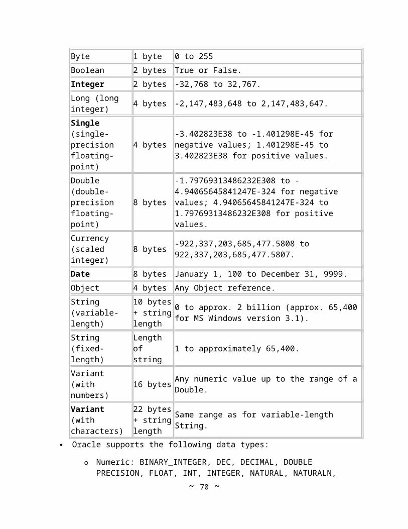
SELECT * FROM avg_sal_dept WHERE department = 'Finance';
Data Storage Characteristics:
For a significant amount of data, we require persistent, inexpensive, reliable and sharable storage methods with relatively rapid access time.
Persistent - Data persists (lives on) after power is removed.
Inexpensive - typically measured on a $ per Megabyte basis.
~ 70 ~

Reliable - Should not have to be replaced due to excessive errors.
Sharable - Should facilitate sharing of data among many users.
Access time - Data should be accessible in a relatively short period of time.
Data Storage Hierarchy
Processor Registers 1 - 5 ns $1000's / MB Cache memory 15 - 30 ns $100's / MB Main Memory (Core) 40 - 100 ns $10's / MB Magnetic Disk (hard disk) 5 - 30 ms $1 / MB Optical Disk (CD-ROM) 50 - 100 ms $1 / GB Magnetic Tape 100's ms to seconds less than $1 / GB
Magnetic Disk Characteristics
We focus on magnetic disk Access time is the dominant cost to consider
Access time consists of:
1. Seek time - moving the disk read/write head to the right track
2. Disk Rotation time - waiting for the disk to rotate the track under the head
3. Transfer time - time to actually read the data (blocks) from the disk and place it on the bus for main memory.
The goal is to minimize seek and disk rotation delay by orienting related data on the same or adjacent tracks.
Block - The smallest unit of memory a disk can read or write.
Block Size - the size of the block. Typically 512 bytes, 1024, 2048, ... 32 Kilobytes.
Record Storage on Disk
Relations (records) are stored on disk with each tuple written one after the other (end to end).
Blocking Factor - the number of tuples (records) that can fit into a single block.
Example: EMPLOYEE takes 100 bytes to store one tuple (record).If the Block Size is 2,000 bytes, then we can store 20 EMPLOYEE tuples (records) in one block.Thus the Blocking factor is 2000/100 = 20
f = B/R
~ 71 ~
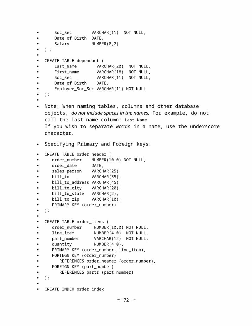
Fixed length records: Each record is of fixed length. Pad with spaces, etc.
Variable Length records: Each record is only as long as the data it contains.
Unspanned Records: A record is found in one and only one block. i.e., records do not span across block boundaries.
Spanned Records: Records are allowed to span across block boundaries.
File Operations
Consider four basic File Operations:
Operation Similar SQL Statement
Find Select
Insert Insert
Modify Update
Delete Delete
Unordered file - New record is inserted at the end of the file.
o Insert takes constant time.
o Select, Update and Delete take n/2 time.(n is the number of records)
Ordered file - New record is inserted in order, in the file.
o Insert takes log2n plus this time to re-organize records.
o Select, Update, Delete take at least log2n
Indexed file - New record is inserted at the end of the file.
o An index is maintained that points to the location on disk where the record is found.
o Insert takes constant time for the data itself plus log2n for the index
o Select, Update, Delete take log2n lookup on the index followed by constant time to access data record.
Types of Indexing
An index is made up of two components: A key and a pointer
~ 72 ~
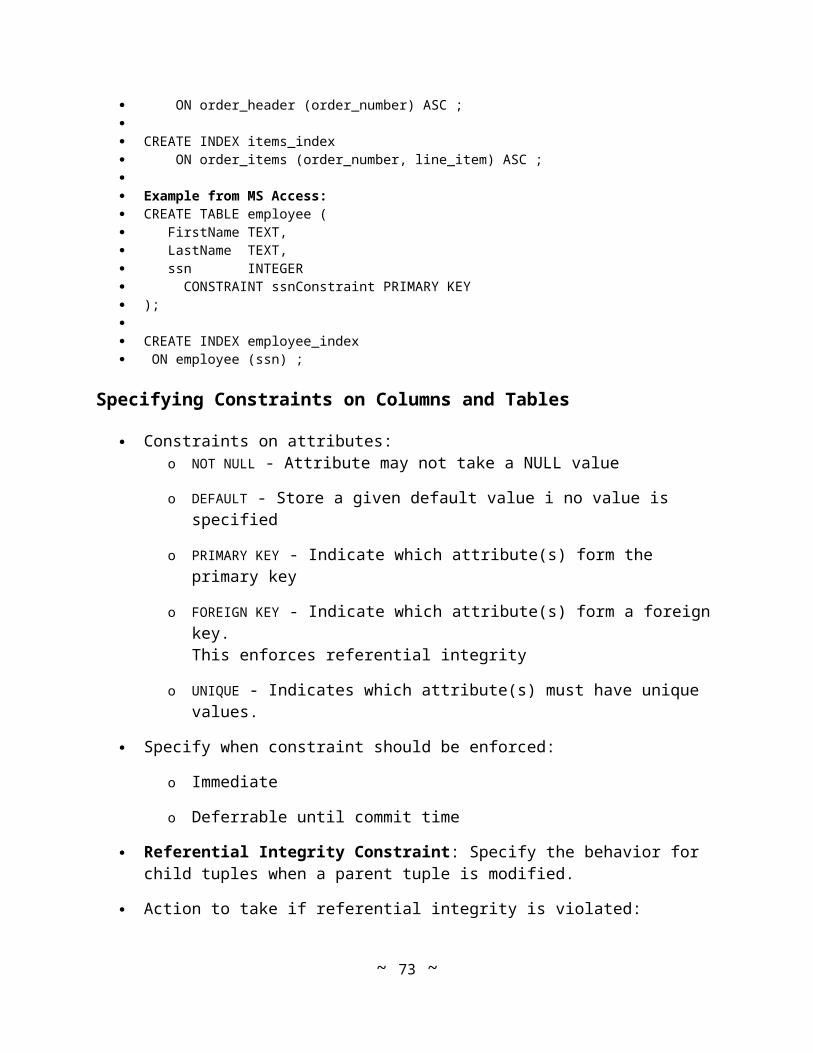
The key is typically the key value for the relation and is mainly used to identify and look up records.
The pointer is an address on disk where the rest of the data in the record can be found.
Two types of indexes discussed here: Ordered index and Hashing.
Ordered Index
Records are stored as they are inserted. Key attribute is stored in order in the index.
Hashing
Identify a function f that takes as input, the key for a relation and returns, as output, the physical disk address for the rest of the data in the record.
Example: Assume employee records.Function f takes the ascii values of the first and last name and adds them.The numeric result is the physical address for the record.
Selection time is constant.
It is possible function f can map two different keys to the same address. In this case, we use a series of hash buckets.
~ 73 ~
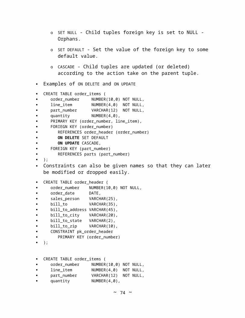
Database System Architectures:
There are a number of database system architectures presently in use. One must examine several criteria:
1. Where do the data and DBMS reside ?
2. Where are the application program executed (e.g., which CPU) ? This may include the user interface.
3. Where are business rules enforced ?
Traditional Mainframe Architecture
Database (or files) resides on a mainframe computer. Applications are run on the same mainframe computer. e.g., COBOL programs or JCL
scripts that access the database.
Business rules are enforced in the applications running on the mainframe.
Multiple users access the applications through simple terminals (e.g., IBM 3270 terminals or VT220 terminals) that have no processing power of their own. User interface is text-mode screens.
Example: DB2 database and COBOL application programs running on an IBM 390.
Advantages:
o Excellent security and control over applications
o High reliability - years of proven MF technology
o Relatively low incremental cost per user (just add a terminal)
Disadvantages:
~ 74 ~
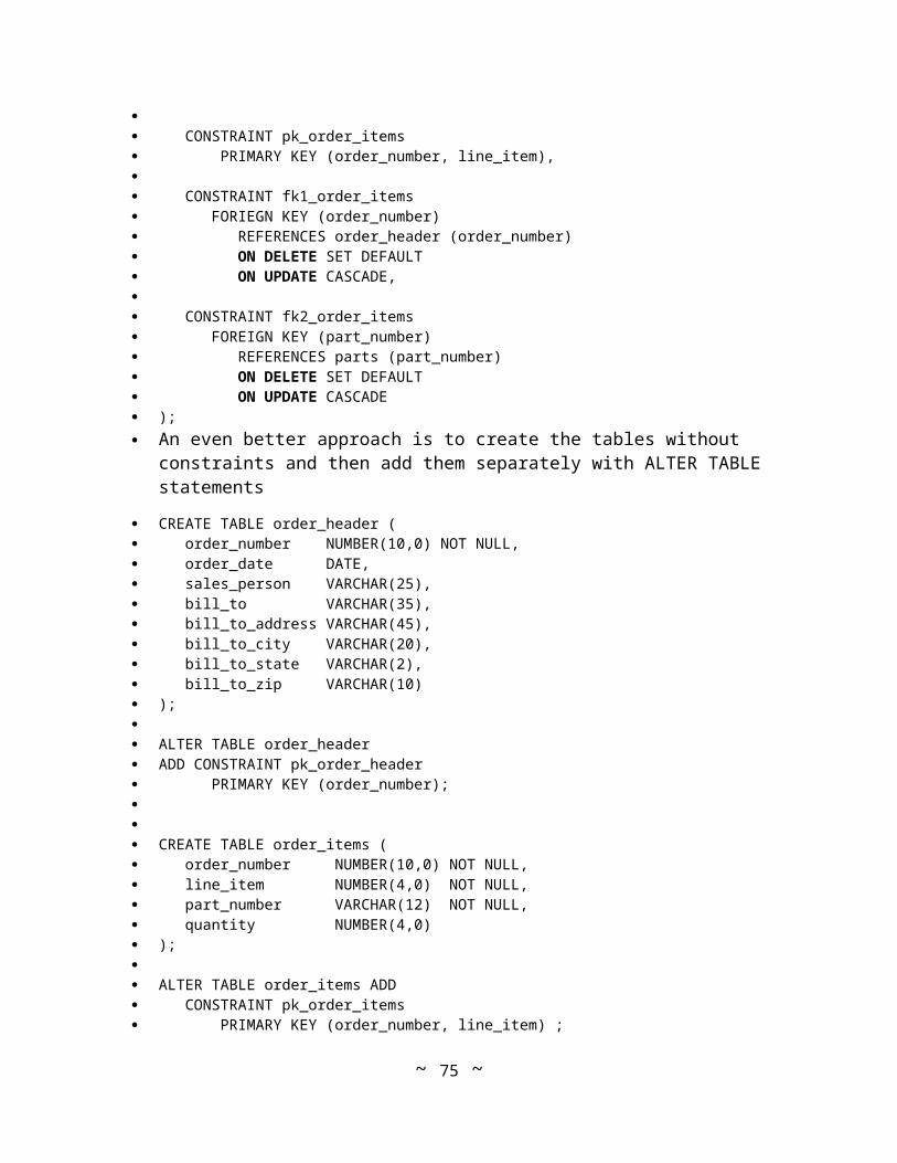
o Unable to effectively serve advanced user interfaces
o Users unable to effectively manipulate data outside of standard applications
Personal Computer - Stand-Alone Database
Database (or files) reside on a PC - on the hard disk. Applications run on the same PC and directly access the database. In such cases, the
application is the DBMS.
Business rules are enforced in the applications running on the PC.
A single user accesses the applications.
Example: MS Access running on a PC.
~ 75 ~

File Sharing Architecture
PCs are connected to a local area network (LAN). A single file server stores a single copy of the database files.
PCs on the LAN map a drive letter (or volume name) on the file server.
Applications run on each PC on the LAN and access the same set of files on the file server. The application is also the DBMS.
Business rules are enforced in the applications - Also, the applications must handle concurrency control. Possibly by file locking.
Each user runs a copy of the same application and accesses the same files.
Example: Sharing MS Access files on a file server.
Advantages:
o (limited) Ability to share data among several users
o Costs of storage spread out among users
o Most components are now commodity items - prices falling
Disadvantages:
o Limited data sharing ability - a few users at most
~ 76 ~
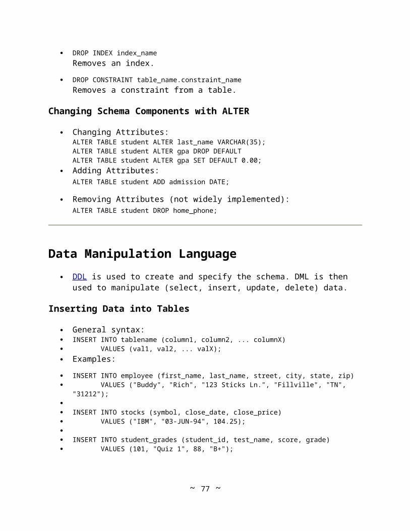
Classic Client/Server Architecture
Client machines: o Run own copy of an operating system.
o Run one or more applications using the client machine's CPU, memory.
o Application communicates with DBMS server running on server machine through a Database Driver
o Database driver (middleware) makes a connection to the DBMS server over a network.
o Examples of clients: PCs with MS Windows operating system. Forms and reports developed in: PowerBuilder, MS Access, Borland Delphi, Oracle Developer, MS Visual Basic, "C" or "C++", etc.
Server Machines:
o Run own copy of an operating system.
o Run a Database Management System that manages a database.
o Provides a Listening daemon that accepts connections from client machines and submits transactions to DBMS on behalf of the client machines.
o Examples: Sun Sparc server running UNIX operating system. RDBMS such as Oracle Server, Sybase, Informix, DB2, etc.PC with Windows operating system.
Middleware:
o Small portion of software that sits between client and server.
~ 77 ~

o Establishes a connection from the client to the server and passes commands (e.g., SQL) between them.
o See ODBC below.
o Examples: For Oracle: SQL*Net (or Net8) running on both client and server.For Sybase: Sybase Open Client and Open Server.
Business rules may be enforced at:
1. The client application - so called "Fat Clients".
2. Entirely on the database server - so called "Thin Clients"
3. A Mix of both.
Advantages of client/server:
1. Processing of the entire Database System is spread out over clients and server.
2. DBMS can achieve high performance because it is dedicated to processing transactions (not running applications).
3. Client Applications can take full advantage of advanced user interfaces such as Graphical User Interfaces.
Disadvantages of client/server:
1. Implementation is more complex because one needs to deal with middleware and the network.
2. It is possible the network is not well suited for client/server communications and may become saturated.
3. Additional burden on DBMS server to handle concurrency control, etc.
4. As more business rule logic is programmed into the client side applications, they can become unwieldy. Stored procedures and triggers can help in this case.
Example: Oracle RDBMS running on a server. Sybase PowerBuilder running on a client PC.
~ 78 ~

Distributed Database Architecture
In a distributed database system (DDS), multiple Database Management Systems run on multiple servers (sites) connected by a network.
Data may be split up among the different servers or it may be replicated.
Data Partitioning
Data may be split up (or partitioned) in several ways: 1. Horizontal: Rows in a table are split up across multiple sites. 2. Vertical: Columns in a table are split across multiple sites.
3. Both vertical and horizontal.
Splitting up data can improve performance by reducing contention for tables.
~ 79 ~

Customer Table
Customer ID Name Address City State Zip
1001 Mr. Smith 123 Lexington Smithville KY 91232
1002 Mrs. Jones 12 Davis Ave. Smithville KY 91232
1003 Mr. Axe 443 Grinder Ln. Broadville GA 81992
1004 Mr. Builder 661 Parker Rd. Streetville GA 81990
Horizontal Partitioning:
Partition 1 Customer ID Name Address City State Zip1001 Mr. Smith 123 Lexington Smithville KY 912321002 Mrs. Jones 12 Davis Ave. Smithville KY 91232
Partition 2 Customer ID Name Address City State Zip1003 Mr. Axe 443 Grinder Ln. Broadville GA 81992 1004 Mr. Builder 661 Parker Rd. Streetville GA 81990
Vertical Partitioning:
Partition 1 CustID Name 1001 Mr. Smith1002 Mrs. Jones1003 Mr. Axe1004 Mr. Builder
Partition 2 CustID Address City State Zip1001 123 Lexington Smithville KY 912321002 12 Davis Ave. Smithville KY 912321003 443 Grinder Ln. Broadville GA 81992 1004 661 Parker Rd. Streetville GA 81990
Data Replication
Data may also be replicated across multiple sites: 1. Improve performance by moving a copy of data closer to the users.
2. Improve reliability - if one site fails, others can continue processing the transactions.
We need mechanisms in place to ensure multiple copies of data are kept consistent.
Recall in a centralized DB we had the notion of a commit point. In distributed DB, we need to consider committing a transaction that changes data on multiple sites.
Distributed Commit Protocol such as Two Phase Commit (2PC). Also called a synchronous replication protocol.
1. Phase 1: Send a message to all sites: "Can you commit Transaction X?" All sites that can commit this transaction reply with "Y".
~ 80 ~

2. Phase 2: If all sites reply with "Y", then send a "Commit" message to all sites.If any site replies "No", then the transaction is aborted.
2PC is an example of a synchronous replication protocol.
In Asynchronous replication, we take snapshots of a master database and propagate the changes to other sites on some periodic basis.
In general, distributed database systems offer more flexibility, higher performance and greater levels of independence over centralized systems.
However, distributed database systems are also much harder to design and develop, control and administrate. Security is also more difficult to enforce.
BTW, for those of you from the UNIX world, simply replace "PCs" with "UNIX Workstations" in the phrases above.
Open DataBase Connectivity (ODBC)
Middleware has historically been proprietary. Note also subtle differences in SQL and how it is implemented in various DBMS.
How can a single client access multiple DBMS servers with minimal changes ?
ODBC is middleware software that can connect a client to multiple servers from different vendors.
ODBC has two main portions that reside on the client: A Driver Manager and one or more DBMS drivers.
The Driver Manager presents a uniform interface to all clients. This consists of a set of function calls to query, update and manipulate data on a server
A DBMS Driver is typically supplied by the individual DBMS vendor and contains routines to convert requests from the Driver Manager into commands the specific DBMS understands.
Try this: Visit several DBMS vendor's web sites and see if they offer an ODBC driver that can be downloaded to your PC.
~ 81 ~

Triggers and Stored Procedures
Triggers are procedures or functions stored in the DBMS and are invoked when certain events occur.
Events include: Inserting a new row into a table, updating data in a table, deleting a row in a table, etc.
Example: A trigger may fire after each time an inventory record is updated. The trigger will automatically insert a new Order record in the Orders table if the quantity in inventory falls below a certain level.
Triggers are used to enforce business rules that all applications that use the database must adhere to.
Programming triggers requires special attention is paid to how transaction execute. Triggers may cause locks to be held longer than expected or may have other side effects.
Most major DBMS support triggers. e.g., Oracle supports triggers written in PL/SQL. IBM DB2 supports triggers written in just about any language such as "C" and Java.
Stored Procedures are similar to triggers: They are functions and procedures that are stored in the database. Stored procedures may be called by triggers or by application programs.
Stored procedures are useful in cases when standard applications logic must be implemented across all applications. Copies of this code do not need to be distributed to the clients.
Also very useful when a large number of database accesses must be done with just a small result being passed back to the client.
~ 82 ~

Internet and Intranet Databases
Companies are discovering that database can provide excellent content for web pages. Many examples: Retail store with current products and price lists, On-line banking-
banks with account balance information, Employee directories, etc.
Several approaches to making database data available on-line:
1. Periodically dump a database table to an HTML file and make the HTML file available on the web (e.g., MS Access Internet Wizard).
2. Provide a mechanism to query the database in real time and format the results in HTML.
3. Provide the web user with a form or other means to invoke a query on the database in real time. Results are formatted in HTML and returned to the user's browser.
The latter 2 are similar. The difference is in the last one, users can specify some or all of the query.
There are two main ways to carry out dynamic real-time queries from the web:
1. Using traditional HTML forms, information is passed to a CGI script that formats the query and submits it to the DBMS. Results are returned to the CGI script which then formats the output in HTML.One needs: An HTTP (web) server, some language (e.g., Perl) that supports CGI, middleware to connect to the database, the DBMS.By far this is the predominant method.
2. Many DBMS now have the web server built in (or closely tied) to the database. e.g., Oracle Web Applications Server.Stored procedures in the DBMS are used to accept input from HTML forms, perform the appropriate query and then format the results in HTML.
~ 83 ~

MultiUser Databases:
Multiuser database - more than one user processes the database at the same time Several issues arise:
1. How can we prevent users from interfering with each other's work ?
2. How can we safely process transactions on the database without corrupting or losing data ?
3. If there is a problem (e.g., power failure or system crash), how can we recover without loosing all of our data ?
Transaction Processing
We need the ability to control how transactions are run in a multiuser database. A transaction is a set of read and write operations that must either commit or abort.
Consider the following transaction that reserves a seat on an airplane flight and changes the customer:1. Read customer information2. Write reservation information3. Write charges
Suppose that after the second step, the database crashes. Or for some reason, changes can not be written...
Transactions can either reach a commit point, where all actions are permanently saved in the database or they can abort in which case none of the actions are saved.
Another way to say this is transactions are Atomic. All operations in a transaction must be executed as a single unit - Logical Unit of Work.
Consider two users, each executing similar transactions:
Example #1: User A User B Read Salary for emp 101 Read Salary for emp 101 Multiply salary by 1.03 Multiply salary by 1.04 Write Salary for emp 101 Write Salary for emp 101
~ 84 ~

Example #2: User A User B Read inventory for Prod 200 Read inventory for Prod 200 Decrement inventory by 5 Decrement inventory by 7 Write inventory for Prod 200 Write inventory for Prod 200
First, what should the values for salary (in the first example) really be ?
The DBMS must find a way to execute these two transactions concurrently and ensure the result is what the users (and designers) intended.
These two are examples of the Lost Update or Concurrent Update problem. Some changes to the database can be overwritten.
Consider how the operations for user's A and B might be interleaved as in example #2. Assume there are 10 units in inventory for Prod 200:
Read inventory for Prod 200 for user A Read inventory for Prod 200 for user B Decrement inventory by 5 for user A Decrement inventory by 7 for user B Write inventory for Prod 200 for user A Write inventory for Prod 200 for user B
Or something similar like:
Read inventory for Prod 200 for user ADecrement inventory by 5 for user AWrite inventory for Prod 200 for user ARead inventory for Prod 200 for user BDecrement inventory by 7 for user BWrite inventory for Prod 200 for user B
In the first case, the incorrect amount (3) is written to the database. This is called the Lost Update problem because we lost the update from User A - it was overwritten by user B.
The second example works because we let user A write the new value of Prod 200 before user B can read it. Thus User B's decrement operation will fail.
Here is another example. User's A and B share a bank account. Assume an initial balance of $200.
User A reads the balance User A deducts $100 from the balance User B reads the balance User A writes the new balance of $100 User B deducts $100 from the balance User B writes the new balance of $100
The reason we get the wrong final result (remaining balance of $100) is because transaction B was allowed to read stale data. This is called the inconsistent read problem.
~ 85 ~

Suppose, instead of interleaving (mixing) the operations of the two transactions, we execute one after the other (note it makes no difference which order: A then B, or B then A)
User A reads the balance User A deducts $100 from the balance User A writes the new balance of $100 User B reads the balance (which is now $100) User B deducts $100 from the balance User B writes the new balance of $0
If we insist only one transaction can execute at a time, in serial order, then performance will be quite poor.
Concurrency Control is a method for controlling or scheduling the operations in such a way that concurrent transactions can be executed.
If we do concurrency control properly, then we can maximize transaction throughput while avoiding any chance.
Transaction throughput: The number of transactions we can perform in a given time period. Often reported as Transactions per second or TPS.
A group of two or more concurrent transactions are serializable if we can order their operations so that the final result is the same as if we had run them in serial order (one after another).
Consider transaction A, B, C and D. Each has 3 operations. If executing:A1, B1, A2, C1, C2, B2, A3, B3, C3has the same result as executing:A1, A2, A3, B1, B2, B3, C1, C2, C3Then the above schedule of transactions and operations is serialized.
Concurrency Control and Locking
We need a way to guarantee that our concurrent transactions can be serialized. Locking is one such means.
Locking is done to data items in order to reserve them for future operations.
A lock is a logical flag set by a transaction to alert other transactions the data item is in use.
Characteristics of Locks
Locks may be applied to data items in two ways:Implicit Locks are applied by the DBMSExplicit Locks are applied by application programs.
Locks may be applied to:
1. a single data item (value)
~ 86 ~

2. an entire row of a table
3. a page (memory segment) (many rows worth)
4. an entire table
5. an entire database
This is referred to as the Lock granularity
Locks may be of type types depending on the requirements of the transaction: 1. An Exclusive Lock prevents any other transaction from reading or modifying the
locked item.
2. A Shared Lock allows another transaction to read an item but prevents another transaction from writing the item.
Two Phase Locking
The most commonly implemented locking mechanism is called Two Phased Locking or 2PL. 2PL is a concurrency control mechanism that ensure serializability.
2PL has two phases: Growing and shrinking.
1. A transaction acquires locks on data items it will need to complete the transaction. This is called the growing phase.
2. Once one lock is released, all no other lock may be acquired. This is called the shrinking phase.
Consider our prior example, this time using locks:
User A places an exclusive lock on the balance User A reads the balance User A deducts $100 from the balance User B attempts to place a lock on the balance but fails because A already has an exclusive lock User B is placed into a wait state User A writes the new balance of $100 User A releases the exclusive lock on the balance User B places an exclusive lock on the balance User B reads the balance User B deducts $100 from the balance User B writes the new balance of $100
Here is a more involved example:
User A places a shared lock on item raise_rate User A reads raise_rate User A places an exclusive lock on item Amy_salary User A reads Amy_salary
~ 87 ~

User B places a shared lock on item raise_rate User B reads raise_rate User A calculates a new salary as Amy_salary * (1+raise_rate) User B places an exclusive lock on item Bill_salary User B reads Bill_salary User B calculates a new salary as Bill_salary * (1+raise_rate) User B writes Bill_salary User A writes Amy_salary User A releases exclusive lock on Amy_salary User B releases exclusive lock on Bill_Salary User B releases shared lock on raise_rate User A releases shared lock on raise_rate
Here is another example:
User A places a shared lock on raise_rate User B attempts to place an exclusive lock on raise_rate Placed into a wait state User A places an exclusive lock on item Amy_salary User A reads raise_rate User A releases shared lock on raise_rate User B places an exclusive lock on raise_rate User A reads Amy_salary User B reads raise_rate User A calculates a new salary as Amy_salary * (1+raise_rate) User B writes a new raise_rate User B releases exclusive lock on raise_rate User A writes Amy_salary User A releases exclusive lock on Amy_salary
Deadlock
Locking can cause problems, however. Consider:
User A places an exclusive lock on item 1001 User B places an exclusive lock on item 2002 User A attempts to place an exclusive lock on item 2002 User A placed into a wait state User B attempts to place an exclusive lock on item 1001 User B placed into a wait state ...
~ 88 ~

This is called a deadlock. One transaction has locked some of the resources and is
waiting for locks so it can complete. A second transaction has locked those needed items but is awaiting the release of locks the first transaction is holding so it can continue.
Two main ways to deal with deadlock.
1. Prevent it in the first place by giving each transaction exclusive rights to acquire all locks needed before proceeding.
2. Allow the deadlock to occur, then break it by aborting one of the transactions.
Database Recovery and Backup
There are many situations in which a transaction may not reach a commit or abort point. 1. An operating system crash can terminate the DBMS processes
2. The DBMS can crash
3. The system might lose power
4. A disk may fail or other hardware may fail.
5. Human error can result in deletion of critical data.
In any of these situations, data in the database may become inconsistent or lost.
Database Recovery is the process of restoring the database and the data to a consistent state. This may include restoring lost data up to the point of the event (e.g. system crash).
Two approaches are discussed here: Reprocessing and Rollback/Rollforward.
Reprocessing
In a Reprocessing approach, the database is periodically backed up (a database save) and all transactions applied since the last save are recorded
If the system crashes, the latest database save is restored and all of the transactions are re-applied (by users) to bring the database back up to the point just before the crash.
Several shortcomings:
1. Time required to re-apply transactions
2. Transactions might have other (physical) consequences
3. Re-applying concurrent transactions is not straight forward.
Automated Recovery with Rollback / Rollforward
~ 89 ~
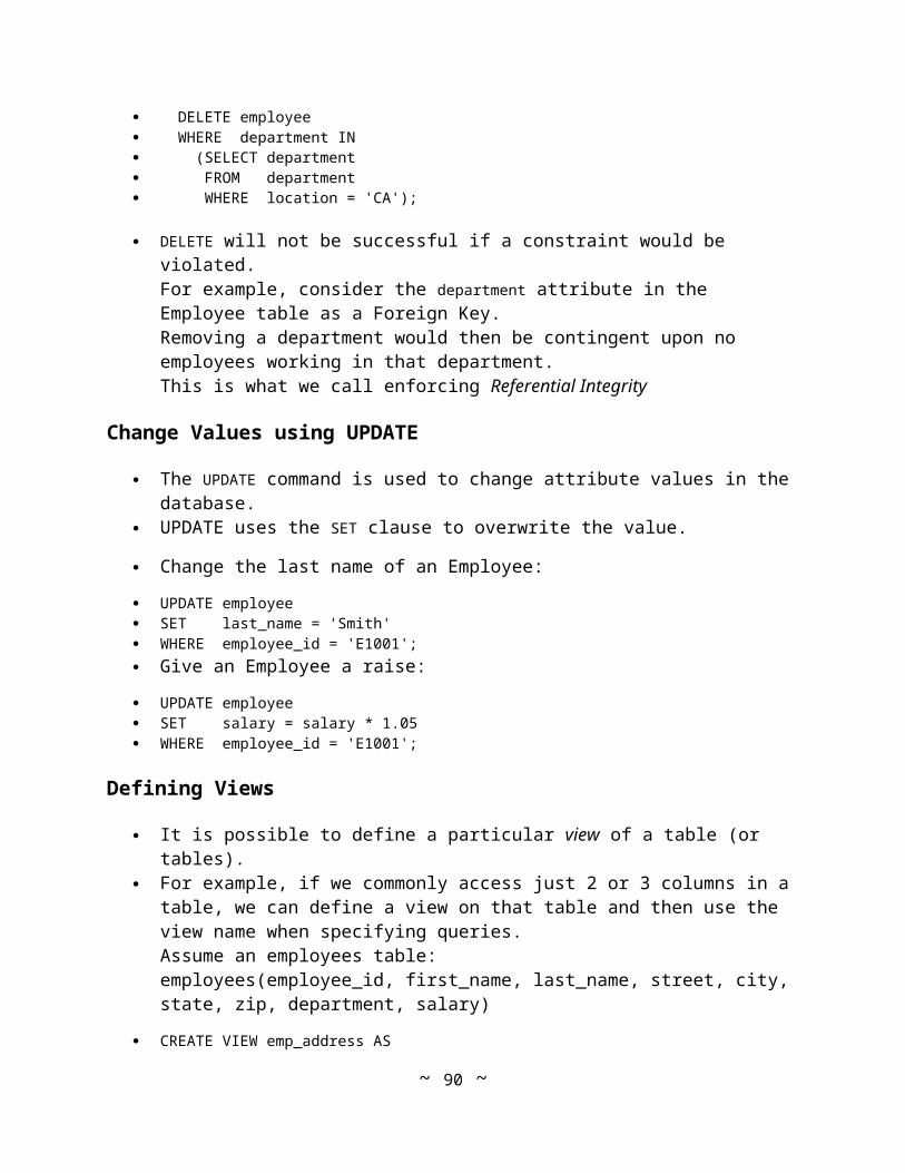
We apply a similar technique: Make periodic saves of the database (time consuming operation). However, maintain a more intelligent log of the transactions that have been applied. This transaction log Includes before images and after images
Before Image: A copy of the table record (or page) of data before it was changed by the transaction.
After Image: A copy of the table record (or page) of data after it was changed by the transaction.
Rollback: Undo any partially completed transactions (ones in progress when the crash occurred) by applying the before images to the database.
Rollforward: Redo the transactions by applying the after images to the database. This is done for transactions that were committed before the crash.
Recovery process uses both rollback and rollforward to restore the database.
In the worst case, we would need to rollback to the last database save and then rollforward to the point just before the crash.
Checkpoints can also be taken (less time consuming) in between database saves.
The DBMS flushes all pending transactions and writes all data to disk and transaction log.
Database can be recovered from the last checkpoint in much less time.
Database Backup
When secondary media (disk) fails, data may become unreadable. We typically rely on backing up the database to cheaper magnetic tape or other backup
medium for a copy that can be restored.
However, when an DBMS is running, it is not possible to backup its files as the resulting backup copy on tape may be inconsistent.
One solution: Shut down the DBMS (and thus all applications), do a full backup - copy everything on to tape. Then start up again.May be infeasible to do often.
Most modern DBMS allow for incremental backups.
An Incremental backup will backup only those data changed or added since the last full backup. Sometimes called a delta backup.
Follows something like:
1. Weekend: Do a shutdown of the DBMS, and full backup of the database onto a fresh tape(s).
~ 90 ~

2. Nightly: Do an incremental backup onto different tapes for each night of the week.
~ 91 ~