Database Systems I

Data Warehousing

2222

INTRODUCTION Increasingly, organizations are analyzing

current and historical data to identify useful patterns and support business strategies (Decision Support).

Emphasis is on complex, interactive, exploratory analysis of very large datasets created by integrating data from across all parts of an enterprise; data is fairly static.

Contrast such On-Line Analytic Processing (OLAP) with traditional On-line Transaction Processing (OLTP): mostly long queries, instead of short update transactions.

3333

DATA WAREHOUSING A Data Warehouse is a collection of data for

the purpose of decision support that is: subject oriented - Data that gives information

about a particular subject instead of about a company's ongoing operations.

Integrated - Data that is gathered into the data warehouse from a variety of sources and merged into a coherent whole.

time variant - All data in the data warehouse is identified with a particular time period.

non volatile - Data is stable in a data warehouse. More data is added but data is never removed. This enables management to gain a consistent picture of the business.

(Source: "What is a Data Warehouse?" W.H. Inmon, Prism, Volume 1, Number 1, 1995).

4444

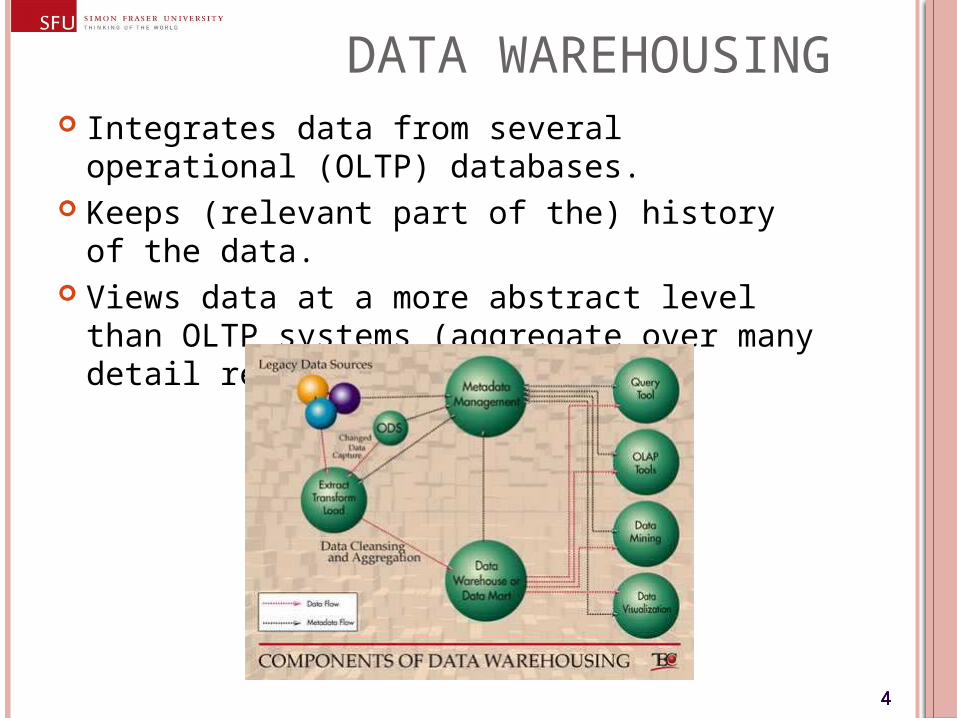
DATA WAREHOUSING Integrates data from several operational

(OLTP) databases. Keeps (relevant part of the) history of the

data. Views data at a more abstract level than OLTP

systems (aggregate over many detail records).

5555

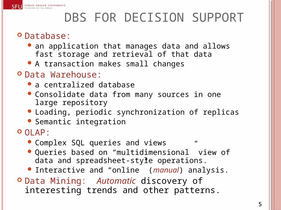
DBS FOR DECISION SUPPORT Database:

an application that manages data and allows fast storage and retrieval of that data

A transaction makes small changes Data Warehouse:

a centralized database Consolidate data from many sources in one large

repository Loading, periodic synchronization of replicas Semantic integration

OLAP: Complex SQL queries and views Queries based on “multidimensional” view of data

and spreadsheet-style operations. Interactive and “online” (manual) analysis.

Data Mining: Automatic discovery of interesting trends and other patterns.

6666

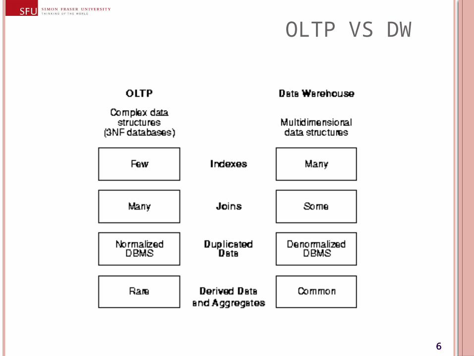
OLTP VS DW

7777

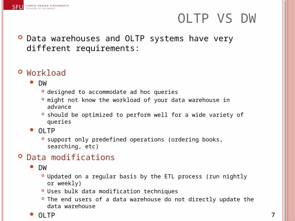
OLTP VS DW Data warehouses and OLTP systems have very different

requirements:

Workload DW

designed to accommodate ad hoc queries might not know the workload of your data warehouse in advance should be optimized to perform well for a wide variety of queries

OLTP support only predefined operations (ordering books, searching, etc)

Data modifications DW

Updated on a regular basis by the ETL process (run nightly or weekly) Uses bulk data modification techniques The end users of a data warehouse do not directly update the data

warehouse OLTP

end users routinely issue individual data modification statements always up to date reflects the current state of each business transaction

8888

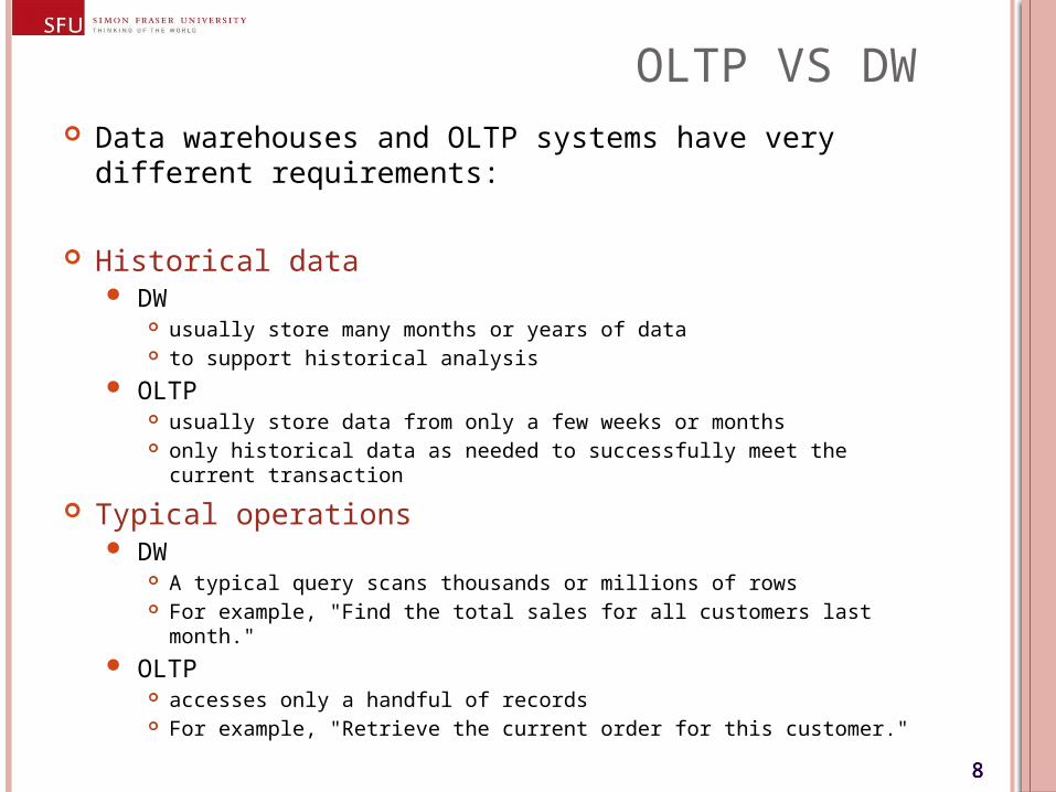
OLTP VS DW Data warehouses and OLTP systems have very different

requirements:

Historical data DW

usually store many months or years of data to support historical analysis

OLTP usually store data from only a few weeks or months only historical data as needed to successfully meet the current

transaction

Typical operations DW

A typical query scans thousands or millions of rows For example, "Find the total sales for all customers last month."

OLTP accesses only a handful of records For example, "Retrieve the current order for this customer."

9999

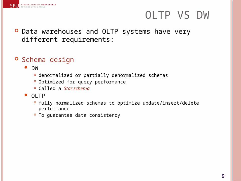
OLTP VS DW Data warehouses and OLTP systems have very different

requirements:

Schema design DW

denormalized or partially denormalized schemas Optimized for query performance Called a Star schema

OLTP fully normalized schemas to optimize update/insert/delete performance To guarantee data consistency

10101010

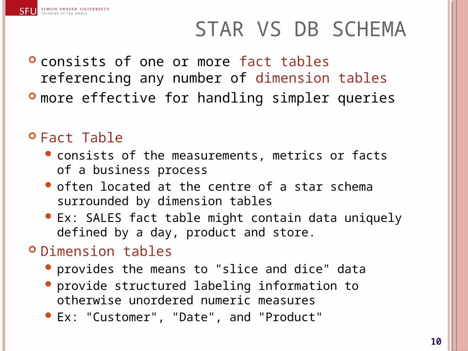
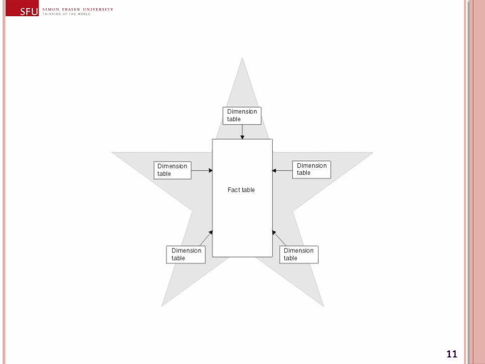
STAR VS DB SCHEMA consists of one or more fact tables referencing

any number of dimension tables more effective for handling simpler queries

Fact Table consists of the measurements, metrics or facts of a

business process often located at the centre of a star schema

surrounded by dimension tables Ex: SALES fact table might contain data uniquely

defined by a day, product and store. Dimension tables

provides the means to "slice and dice" data provide structured labeling information to otherwise

unordered numeric measures Ex: "Customer", "Date", and "Product"

11111111

12121212

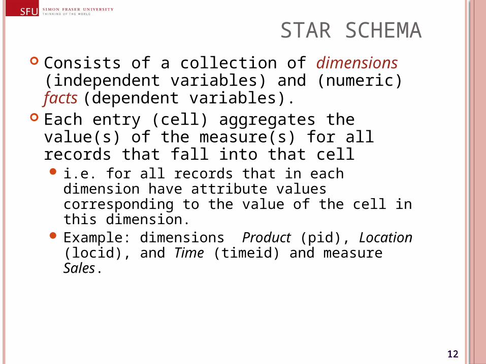
STAR SCHEMA Consists of a collection of dimensions

(independent variables) and (numeric) facts (dependent variables).

Each entry (cell) aggregates the value(s) of the measure(s) for all records that fall into that cell i.e. for all records that in each dimension have

attribute values corresponding to the value of the cell in this dimension.

Example: dimensions Product (pid), Location (locid), and Time (timeid) and measure Sales.

13131313

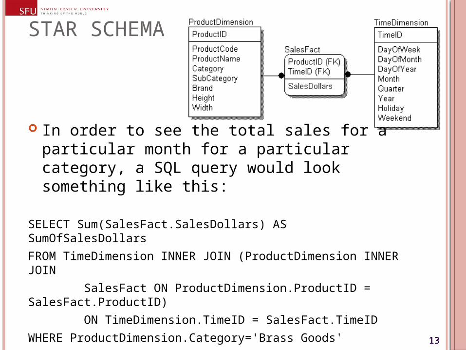
STAR SCHEMA

In order to see the total sales for a particular month for a particular category, a SQL query would look something like this:

SELECT Sum(SalesFact.SalesDollars) AS SumOfSalesDollars

FROM TimeDimension INNER JOIN (ProductDimension INNER JOIN

        SalesFact ON ProductDimension.ProductID = SalesFact.ProductID)

        ON TimeDimension.TimeID = SalesFact.TimeID

WHERE ProductDimension.Category='Brass Goods'

        AND TimeDimension.Month=3

        AND TimeDimension.Year=1999

14141414

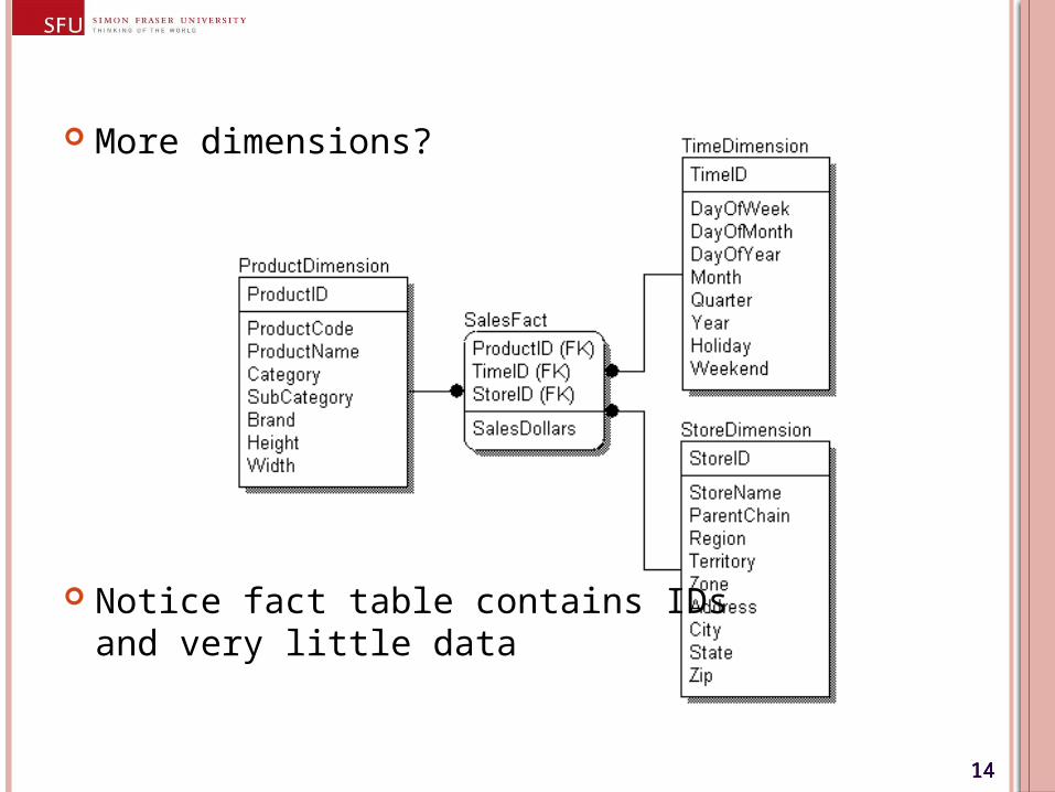
More dimensions?

Notice fact table contains IDsand very little data

15151515

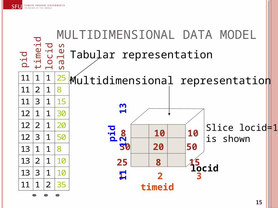
MULTIDIMENSIONAL DATA MODEL

11 1 1 25

11 2 1 8

11 3 1 15

12 1 1 30

12 2 1 20

12 3 1 50

13 1 1 8

13 2 1 10

13 3 1 10

11 1 2 35

pid

tim

eid

loci

dsa

les

8 10 10

30 20 50

25 8 15

1 2 3 timeid

p

id11

12

13

locid

Slice locid=1is shown

Tabular representation

Multidimensional representation

16161616

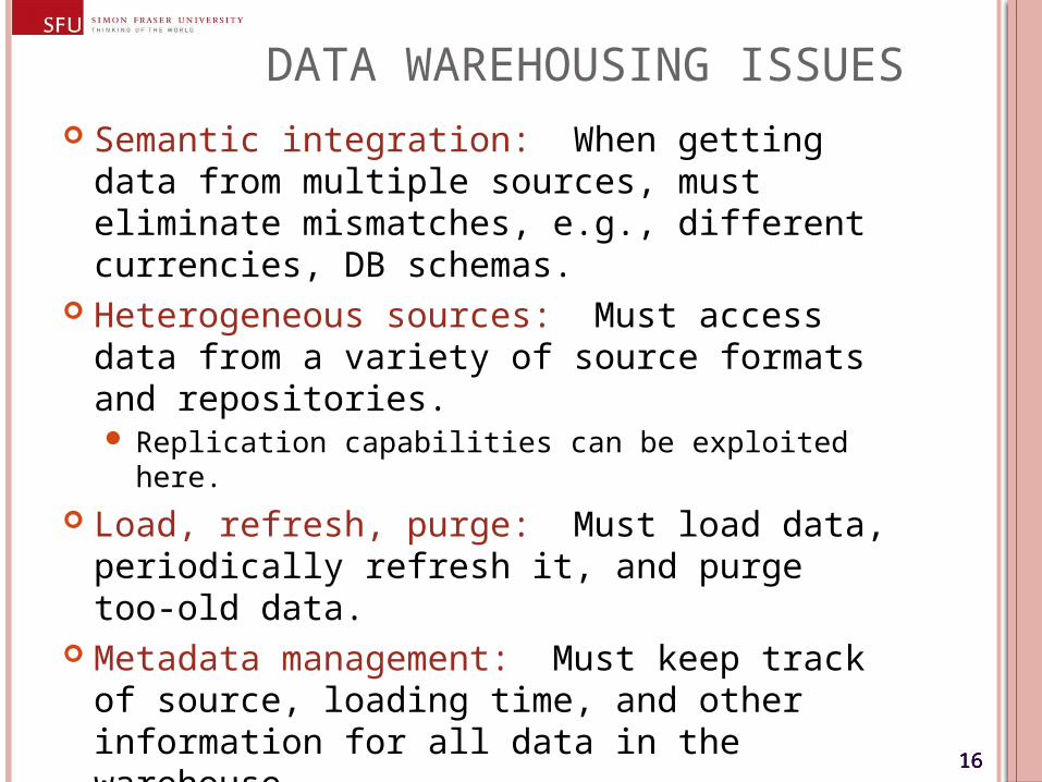
DATA WAREHOUSING ISSUES Semantic integration: When getting data

from multiple sources, must eliminate mismatches, e.g., different currencies, DB schemas.

Heterogeneous sources: Must access data from a variety of source formats and repositories. Replication capabilities can be exploited here.

Load, refresh, purge: Must load data, periodically refresh it, and purge too-old data.

Metadata management: Must keep track of source, loading time, and other information for all data in the warehouse.

DETAILS

18181818

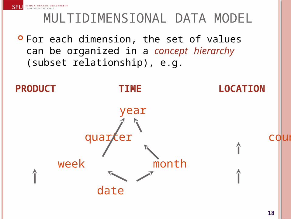
MULTIDIMENSIONAL DATA MODEL For each dimension, the set of values can be

organized in a concept hierarchy (subset relationship), e.g.

PRODUCT TIME LOCATION

category week month state

pname date city

year

quarter country

19191919

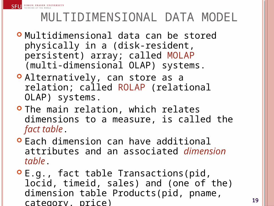
MULTIDIMENSIONAL DATA MODEL Multidimensional data can be stored

physically in a (disk-resident, persistent) array; called MOLAP (multi-dimensional OLAP) systems.

Alternatively, can store as a relation; called ROLAP (relational OLAP) systems.

The main relation, which relates dimensions to a measure, is called the fact table.

Each dimension can have additional attributes and an associated dimension table.

E.g., fact table Transactions(pid, locid, timeid, sales) and (one of the) dimension table Products(pid, pname, category, price)

Fact tables are much larger than dimensional tables.

20202020

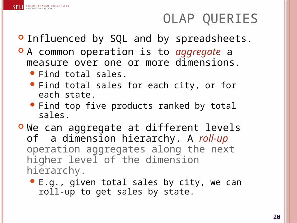
OLAP QUERIES Influenced by SQL and by spreadsheets. A common operation is to aggregate a

measure over one or more dimensions. Find total sales. Find total sales for each city, or for each state. Find top five products ranked by total sales.

We can aggregate at different levels of a dimension hierarchy. A roll-up operation aggregates along the next higher level of the dimension hierarchy. E.g., given total sales by city, we can roll-up to

get sales by state.

21212121

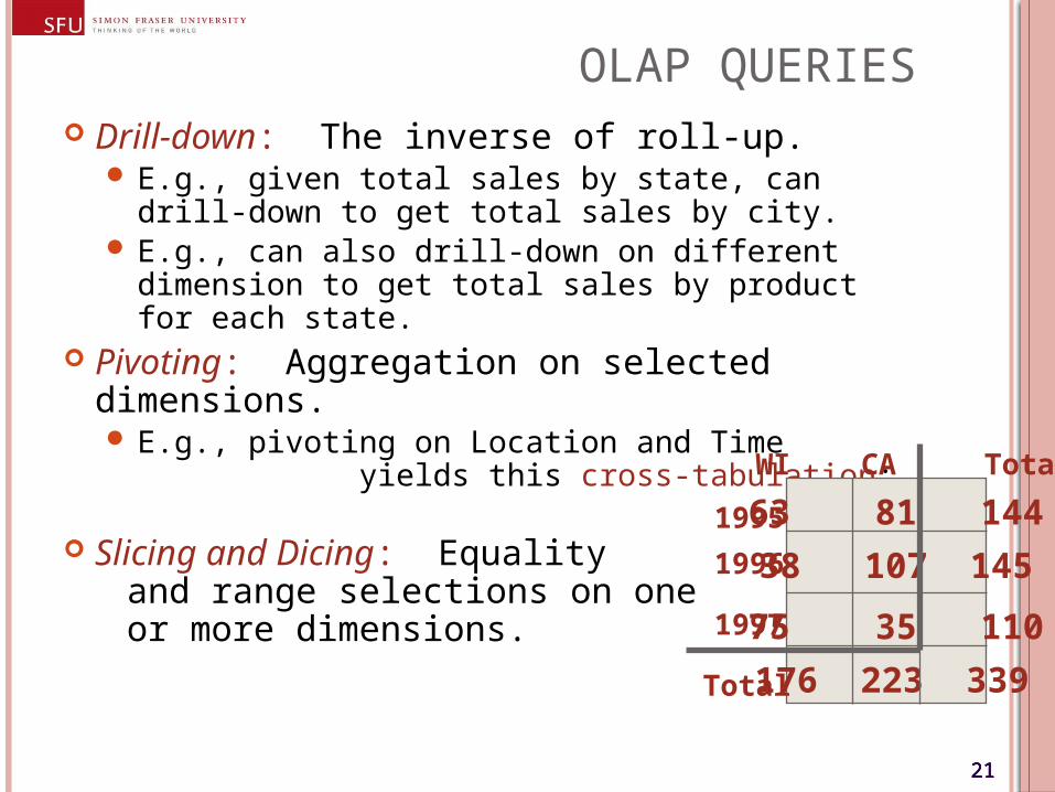
OLAP QUERIES Drill-down: The inverse of roll-up.

E.g., given total sales by state, can drill-down to get total sales by city.

E.g., can also drill-down on different dimension to get total sales by product for each state.

Pivoting: Aggregation on selected dimensions. E.g., pivoting on Location and Time

yields this cross-tabulation:

Slicing and Dicing: Equality and range selections on one or more dimensions.

63 81 144

38 107 145

75 35 110

WI CA Total

1995

1996

1997

176 223 339Total

22222222

DEMO http://www.youtube.com/watch?v=-

j5J7lXav7Y#t=12m30s

From 11:55 to 18:44

23232323

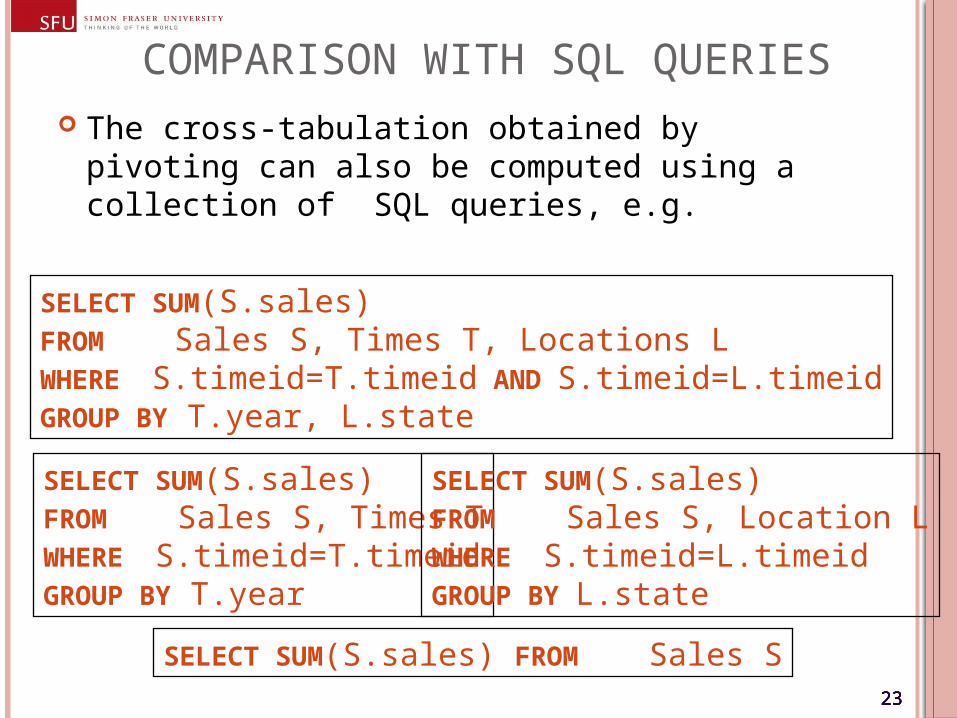
COMPARISON WITH SQL QUERIES The cross-tabulation obtained by pivoting can

also be computed using a collection of SQL queries, e.g.

SELECT SUM(S.sales)FROM Sales S, Times T, Locations LWHERE S.timeid=T.timeid AND S.timeid=L.timeidGROUP BY T.year, L.state

SELECT SUM(S.sales)FROM Sales S, Times TWHERE S.timeid=T.timeidGROUP BY T.year

SELECT SUM(S.sales)FROM Sales S, Location LWHERE S.timeid=L.timeidGROUP BY L.state

SELECT SUM(S.sales) FROM Sales S

24242424

THE CUBE OPERATOR Generalizing the previous example, if there

are d dimensions, we have 2d possible SQL GROUP BY queries that can be generated through pivoting on a subset of dimensions (without considering selections of specific values for certain dimensions).

A Data Cube is a multi-dimensional model of a datawarehouse where the domain of each dimension is extended by the special value „ALL“ with the semantics of aggregating over all values of the corresponding dimension.

25252525

THE CUBE OPERATOR The Cube Operator computes the measures

for all cells (evaluates all possible GROUP BY queries) at the same time.

It can be much more efficiently processed than the set of all corresponding (independent) SQL GROUP BY queries.

Observation: The results of more generalized queries (with fewer GROUP BY attributes) can be derived from more specialized queries (with more GROUP BY attributes) by aggregating over the irrelevant GROUP BY attributes.

26262626

THE CUBE OPERATOR Process more specialised queries first and,

based on their results, determine the outcome of more generalised queries.

Significant reduction of I/O cost, since intermediate results are much smaller than original (fact) table.

27272727

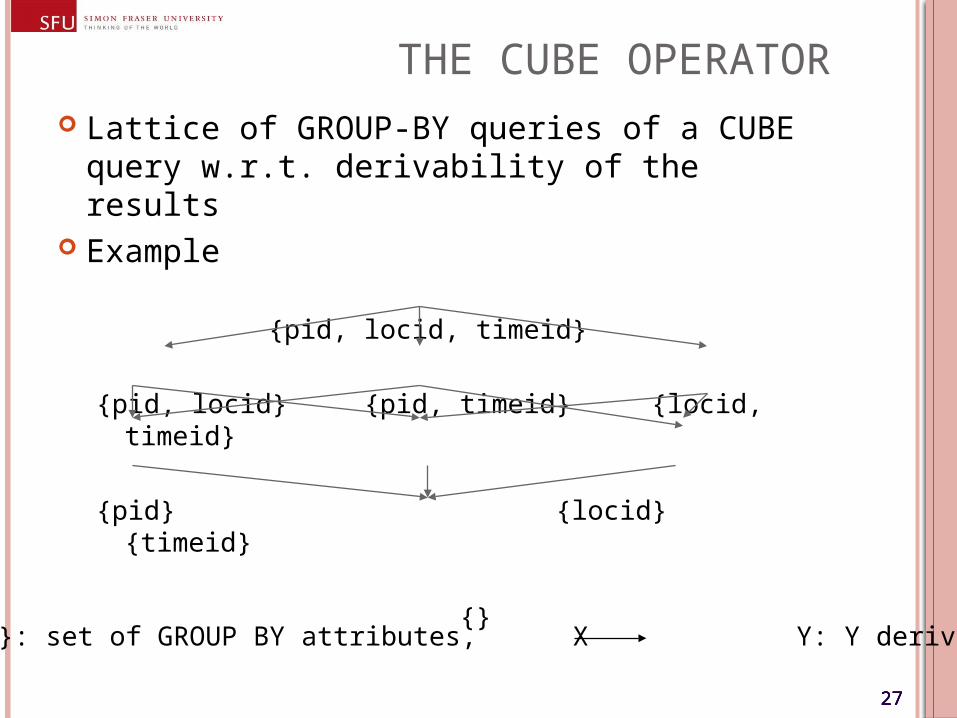
THE CUBE OPERATOR Lattice of GROUP-BY queries of a CUBE query

w.r.t. derivability of the results Example

{pid, locid, timeid}

{pid, locid} {pid, timeid} {locid, timeid}

{pid} {locid} {timeid}

{}

{A,B,. . .}: set of GROUP BY attributes, X Y: Y derivable from X

28282828

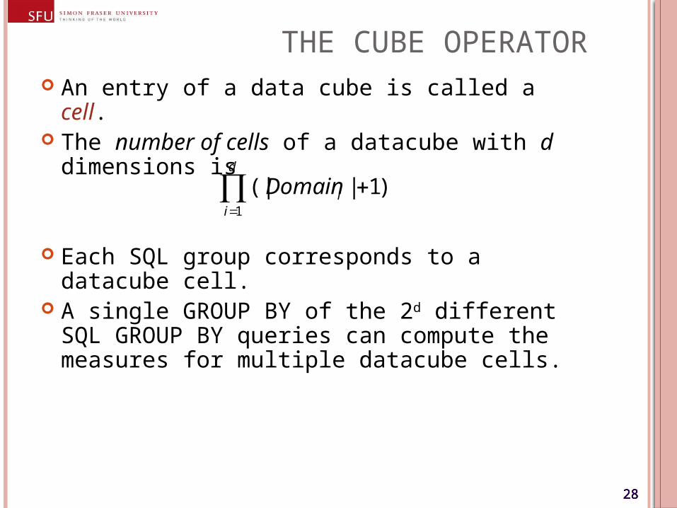
THE CUBE OPERATOR An entry of a data cube is called a cell. The number of cells of a datacube with d

dimensions is

Each SQL group corresponds to a datacube cell.

A single GROUP BY of the 2d different SQL GROUP BY queries can compute the measures for multiple datacube cells.

)1|(|1

d

iiDomain

IMPLEMENTATION ISSUES

30303030

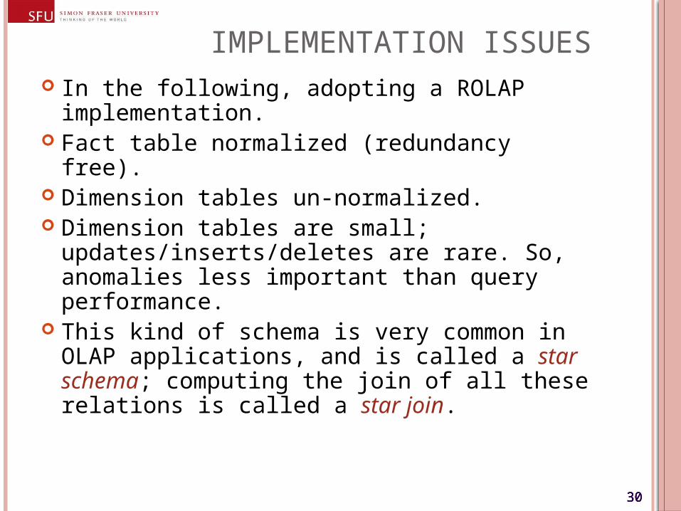
IMPLEMENTATION ISSUES In the following, adopting a ROLAP

implementation. Fact table normalized (redundancy free). Dimension tables un-normalized. Dimension tables are small;

updates/inserts/deletes are rare. So, anomalies less important than query performance.

This kind of schema is very common in OLAP applications, and is called a star schema; computing the join of all these relations is called a star join.

31313131

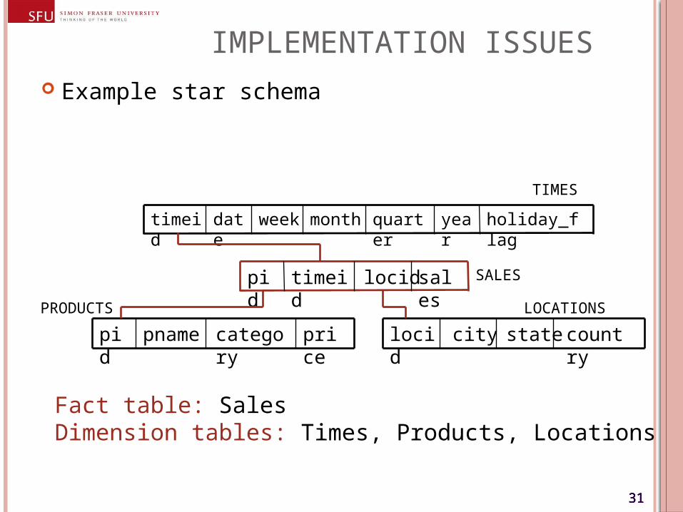
IMPLEMENTATION ISSUES Example star schema

price

category

pname

pid country

statecitylocid

sales

locidtimeid

pid

holiday_flag

weekdate

timeid month

quarter

year

SALES

TIMES

PRODUCTS LOCATIONS

Fact table: SalesDimension tables: Times, Products, Locations

32323232

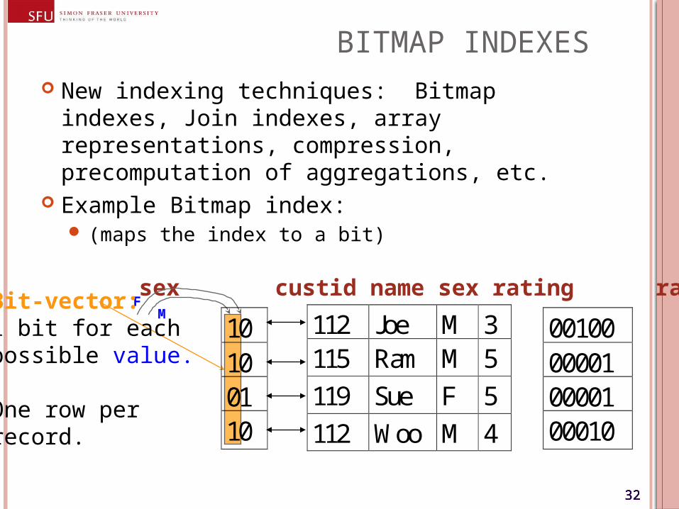
BITMAP INDEXES New indexing techniques: Bitmap indexes,

Join indexes, array representations, compression, precomputation of aggregations, etc.

Example Bitmap index: (maps the index to a bit)

10100110

112 Joe M 3115 Ram M 5

119 Sue F 5

112 Woo M 4

00100000010000100010

sex custid name sex rating ratingM

FBit-vector:1 bit for eachpossible value.

One row per record.

33333333

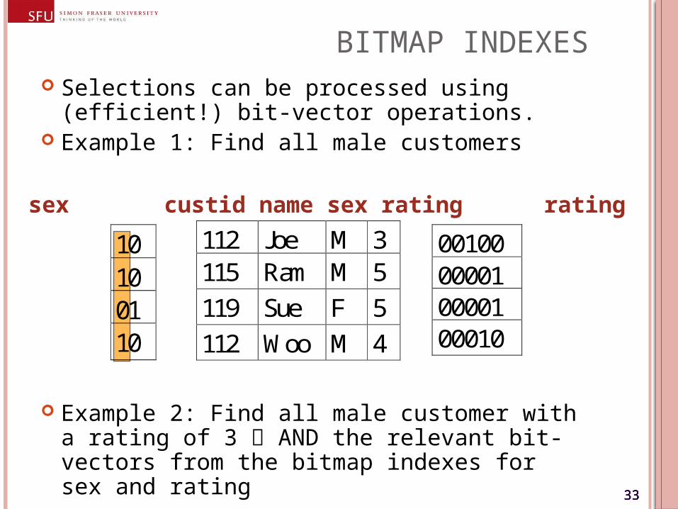
BITMAP INDEXES Selections can be processed using (efficient!)

bit-vector operations. Example 1: Find all male customers

Example 2: Find all male customer with a rating of 3 AND the relevant bit-vectors from the bitmap indexes for sex and rating

10100110

112 Joe M 3115 Ram M 5

119 Sue F 5

112 Woo M 4

00100000010000100010

sex custid name sex rating rating

34343434

JOIN INDEXES Consider the join of Sales, Products, Times,

and Locations, possibly with additional selection conditions (e.g., country=“USA”).

A join index can be constructed to speed up such joins (in a relatively static data warehouse). It basically materializes the result of a join.

The index contains [s,p,t,l] if there are tuples with sid s in Sales, pid p in Products, timeid t in Times and locid l in Locations that satisfy the join (and selection) conditions.

35353535

JOIN INDEXES Problem: Number of join indexes can grow

rapidly. In order to efficiently support all possible

selections in a data cube, you need one join index for each subset of the set of dimensions.

E.g, one join index each for[s,p,t,l], [s,p,t], [s,p,l], [s,t,l], [s,p], [s,t], [s,l]

36363636

BITMAPPED JOIN INDEXES A variation of join indexes addresses this

problem, using the concept of Bitmap indexes.

For each attribute of each dimension table with an additional selection (e.g., country), build a Bitmap index.

Index contains, e.g., entry [c,s] if a dimension table tuple with value c in the selection column joins with a Sales tuple with sid s. Note that s denotes the compound key of the fact table, e.g. [pid, timeid, locid].

The Bitmap index version is especially efficient (Bitmapped Join Index).

Makes sense? Good!

37373737

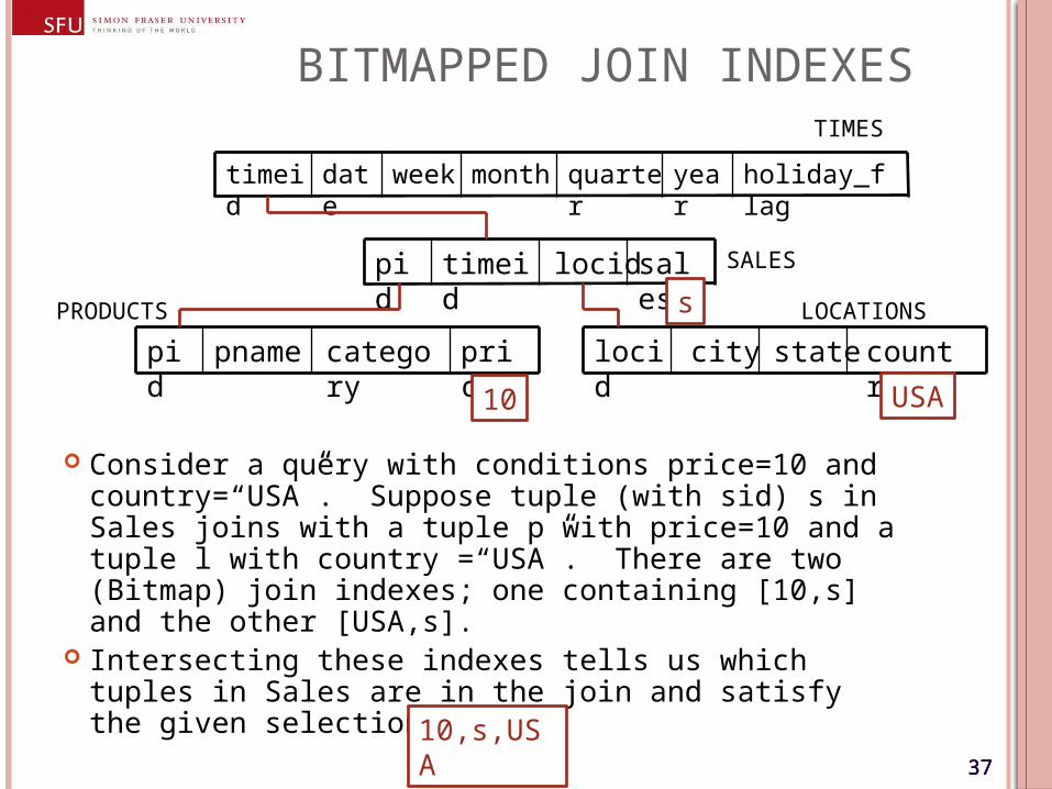
BITMAPPED JOIN INDEXES

Consider a query with conditions price=10 and country=“USA”. Suppose tuple (with sid) s in Sales joins with a tuple p with price=10 and a tuple l with country =“USA”. There are two (Bitmap) join indexes; one containing [10,s] and the other [USA,s].

Intersecting these indexes tells us which tuples in Sales are in the join and satisfy the given selection.

price

category

pname

pid country

statecitylocid

sales

locidtimeid

pid

holiday_flag

weekdate

timeid month

quarter year

SALES

TIMES

PRODUCTS LOCATIONS

10

s

USA

10,s,USA

DIFFERENCES TO STANDARD SQL

39393939

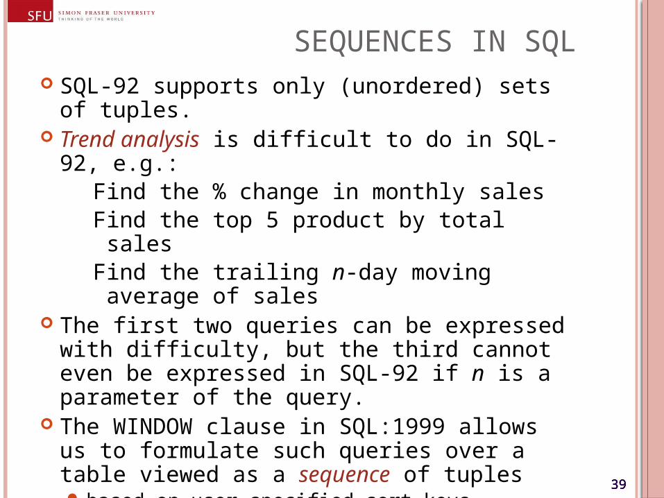
SEQUENCES IN SQL SQL-92 supports only (unordered) sets of

tuples. Trend analysis is difficult to do in SQL-92, e.g.:

Find the % change in monthly salesFind the top 5 product by total salesFind the trailing n-day moving average of sales

The first two queries can be expressed with difficulty, but the third cannot even be expressed in SQL-92 if n is a parameter of the query.

The WINDOW clause in SQL:1999 allows us to formulate such queries over a table viewed as a sequence of tuples based on user-specified sort keys

40404040

THE WINDOW CLAUSE A window is an ordered group of tuples

around each (reference) tuple of a table.

The order within a window is determined based on an attribute specified by the SQL statement.

The width of the window is also specified by the SQL statement.

The tuples of the window can be aggregated using the standard (set-oriented) SQL aggregate functions (SUM, AVG, COUNT, . . .).

41414141

THE WINDOW CLAUSE

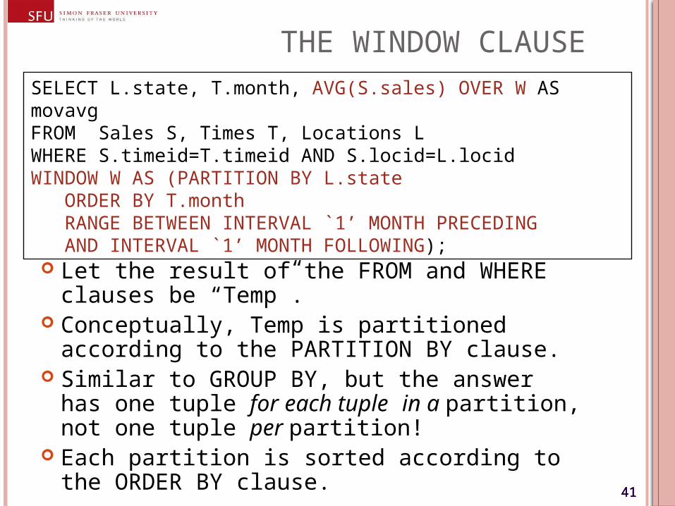
Let the result of the FROM and WHERE clauses be “Temp”.

Conceptually, Temp is partitioned according to the PARTITION BY clause.

Similar to GROUP BY, but the answer has one tuple for each tuple in a partition, not one tuple per partition!

Each partition is sorted according to the ORDER BY clause.

SELECT L.state, T.month, AVG(S.sales) OVER W AS movavgFROM Sales S, Times T, Locations LWHERE S.timeid=T.timeid AND S.locid=L.locidWINDOW W AS (PARTITION BY L.state

ORDER BY T.monthRANGE BETWEEN INTERVAL `1’ MONTH PRECEDINGAND INTERVAL `1’ MONTH FOLLOWING);

42424242

THE WINDOW CLAUSE

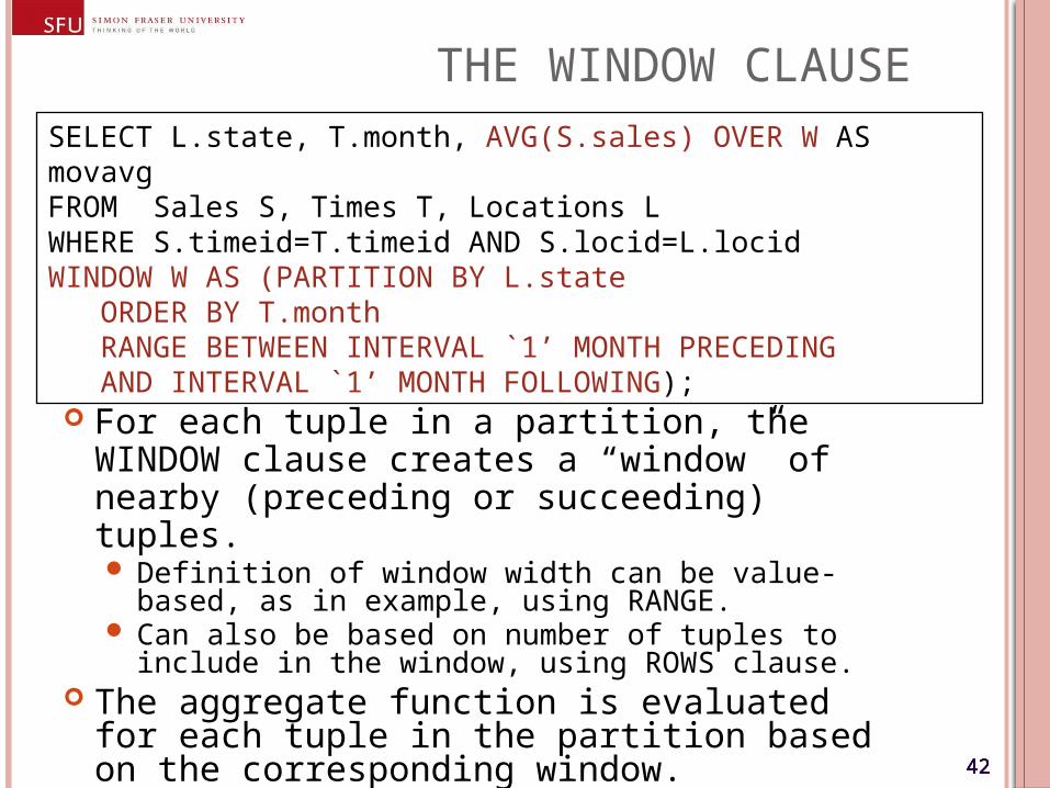
For each tuple in a partition, the WINDOW clause creates a “window” of nearby (preceding or succeeding) tuples. Definition of window width can be value-based, as in

example, using RANGE. Can also be based on number of tuples to include in

the window, using ROWS clause. The aggregate function is evaluated for each

tuple in the partition based on the corresponding window.

SELECT L.state, T.month, AVG(S.sales) OVER W AS movavgFROM Sales S, Times T, Locations LWHERE S.timeid=T.timeid AND S.locid=L.locidWINDOW W AS (PARTITION BY L.state

ORDER BY T.monthRANGE BETWEEN INTERVAL `1’ MONTH PRECEDINGAND INTERVAL `1’ MONTH FOLLOWING);

43434343

TOP N QUERIES Sometimes, want to find only the „best“

answers (e.g., web search engines). If you want to find only the 10 (or so)

cheapest cars, the DBMS should avoid computing the costs of all cars before sorting to determine the 10 cheapest.

Idea: Guess a cost c such that the 10 cheapest cars all cost less than c, and that not too many other cars cost less than c.

Then add the selection cost<c and evaluate the query.

If the guess is right: we avoid computation for cars that cost more than c.

If the guess is wrong: need to reset the selection and recompute the original query.

44444444

TOP N QUERIES

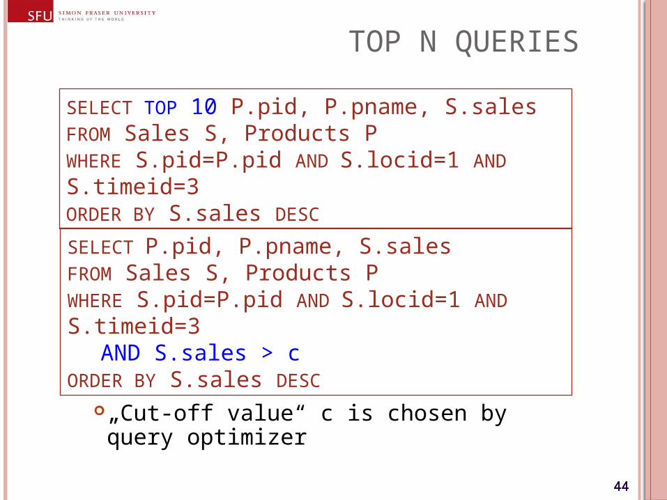
„Cut-off value“ c is chosen by query optimizer

SELECT TOP 10 P.pid, P.pname, S.salesFROM Sales S, Products PWHERE S.pid=P.pid AND S.locid=1 AND S.timeid=3ORDER BY S.sales DESC

SELECT P.pid, P.pname, S.salesFROM Sales S, Products PWHERE S.pid=P.pid AND S.locid=1 AND S.timeid=3

AND S.sales > cORDER BY S.sales DESC

45454545

ONLINE AGGREGATION Consider an aggregate query, e.g., finding the

average sales by state. If we do not have a corresponding

(materialized) data cube, processing this query from scratch can be very expensive.

In general, we have to scan the entire fact table.

But the user expects interactive response time.

An approximate result may be acceptable to the user.

46464646

ONLINE AGGREGATION Can we provide the user with some

approximate results before the exact average is computed for all states?

Can show the current “running average” for each state as the computation proceeds.

Even better, we can use statistical techniques and sample tuples to aggregate instead of simply scanning the aggregated table.

E.g., we can provide bounds such as “the average for Wisconsin is 2000 ± 102 with 95% probability“.