Dating business cycles in India

Radhika Pandey∗ Ila Patnaik

5th January, 2016

Abstract

This paper presents a chronology of Indian business cycle in thepost-reform period. The period before reforms primarily saw monsooncycles. We find three episodes of recession in the post-reform period:1999Q4 to 2003Q1, 2007Q2 to 2009Q3, and 2011Q2 to 2012Q4. Wefind that the average duration of expansion is 12 quarters and theaverage duration of recession is 9 quarters. We find that duration ofexpansions and recessions is similarly diverse. The diversity in dura-tion of expansion is seen to be 0.34 while the diversity in duration ofrecession is 0.31. We find that the amplitude of recession is relativelymore diverse at 0.45 while the diversity in amplitude of expansion is0.38.

∗We thank Joshua Felman for useful comments. Preliminary draft.

1

Contents

1 Introduction 3

2 Indian business cycles 5

3 Methodology 93.1 Seasonal Adjustment and adjustment for outliers . . . . . . . 103.2 Extraction of cycles . . . . . . . . . . . . . . . . . . . . . . . . 103.3 Application of dating algorithm . . . . . . . . . . . . . . . . . 12

4 Empirical analysis 134.1 Business cycle turning points . . . . . . . . . . . . . . . . . . 134.2 Characteristics of turning points: Have the cycles changed

over time? . . . . . . . . . . . . . . . . . . . . . . . . . . . . . 17

5 Sensitivity of turning points chronology: Some robustnesschecks 205.1 Robustness check I: Using Hodrick-Prescott filter . . . . . . . 205.2 Robustness check II: Growth cycle chronology using other ref-

erence series . . . . . . . . . . . . . . . . . . . . . . . . . . . . 22

6 Description of recessions and expansions 23

7 Conclusion 32

A Detrending techniques 33

2

1 Introduction

Stabilising business cycles is a key objective of macroeconomic policy. Under-standing recessions and expansions of business cycles is essential for puttingin place frameworks for stabilisation. This requires identifying the chronol-ogy of business cycle turning points. In the U.S, the National Bureau ofEconomic Research (NBER) has a dedicated research program for identifyingthe dates of business cycle turning points. A number of studies have appliedthe NBER approach to dating the business cycles for developed and emerg-ing economies (Stock and Watson, 1999; Plessis, 2006). Similarly the CEPREuro Area Business Cycle Dating Committee establishes the chronology ofrecessions and expansions of Euro Area member countries. In India therehave been some attempts at determining the chronology of business cycles(Dua and Banerji, 2000; Chitre, 2001; Dua and Banerji, 2001a; Patnaik andSharma, 2002; Mohanty et al., 2003). Majority of these studies focus on thepre-liberalisation period. Business cycle downturns in the pre-liberalisationperiod were associated with drought, or oil price hike and saw sharp declinesin GDP. There were no investment-inventory cycles or periods of expansionfollowed by periods of contraction that are typically seen in industrialisedcountries. This is hardly surprising given the economy was largely a plannedeconomy. There are few studies that extend the business cycle chronologyanalysis to the post reform period (Mohanty et al., 2003; Dua and Banerji,2007). In the post-reform period, an understanding of business cycle chronol-ogy assumes importance as the nature of cycles has changed. After 1991, wehave not seen an actual fall in output like in the pre-reform years but aepisodes of slowdown in the aggregate economic activity.

There are different approaches for measuring business cycles. One approachrefers to “growth cycles,” and relies on detrending procedures to extract thecyclical component of output. The cycle is defined to be in the boom phasewhen actual output is above the estimated trend, and in recession when theactual output is below the estimated trend. The classical approach identifiesexpansion and contraction based on the level of output. In contrast, “growthrate cycle” identifies turning points based on the growth rate of output. Forthe post-reform period in India, growth or growth rate cycle approach ismore appropriate than the classical cycle approach to analyse business cy-cle turning points (Mohanty et al., 2003; Dua and Banerji, 1999, 2007). Inour analysis we use the growth cycle approach and examine the componentadjusted for trend to detect turning points. To isolate the cyclical compo-nent we use the filter by Christiano and Fitzgerald (2003). The Christianoand Fitzgerald (2003) filter belongs to the category of band-pass filters. The

3

band-pass filters extract cycles of a chosen frequency. We extract cycles usingthe NBER business cycle periodicity of 2-8 years. We check the robustnessof our findings by extracting cycles using the Hodrick-Prescott filter (Ho-drick and Prescott, 1997). To the cyclical component we apply the datingalgorithm developed by Bry and Boschan (1971) and improved by Hardingand Pagan (2002). The dating algorithm provides; among others, rules forminimum duration of phase and a complete cycle. The application of thedating algorithm to our dataset gives dates of peaks, troughs and averageduration and amplitude of expansions and recessions.

We use seasonally adjusted quarterly GDP series from 1996 to 2014 to arriveat a chronology of business cycles. We find three episodes of recession. Thefirst period of recession was from the period 1999Q4 to 2003Q1. The secondperiod of recession was from 2007Q2 to 2009 Q3. The third episode of reces-sion began in 2011 Q2 till 2012Q4. Our findings on business cycle chronologyare robust to the choice of filter and to the choice of the measure of businesscycle indicator. The average duration of expansion in India is seen to be 12quarters while the average duration of recession is 9 quarters.

In recent decades, a number of emerging economies have undergone changesin policy environment resulting in structural transformation. One majorstrand of business cycle literature examines the changes in business cyclestylised facts in response to structural transformation (Kim et al., 2003; Alpet al., 2012; Ghate et al., 2013). The main conclusion of these studies isthat emerging economy business cycle facts have changed in the post-reformperiod. We build on this literature by offering evidence of change in theaverage duration of cycle. We also show that the phases of expansion and re-cession have become relatively more diverse in the post-reform period. Usinga longer time series of IIP, we report evidence of both these changes.

The rest of the paper is organised as follows. Section 2 presents a discussionof the changing nature of Indian business cycles and provides an overviewof studies on Indian business cycles. Section 3 outlines the methodology fordetection of turning points, Section 4 presents the empirical analysis and ourfindings on growth cycle turning points. Section 5 assesses the robustness ofour findings on business cycle chronology to the choice of the filter and tothe choice of the reference series. Section 6 presents a brief description of thephases of expansion and recession identified using the dating methodology.Section 7 concludes the paper and outlines areas for future research.

4

Table 1 Sectoral share (Expressed as a % to GDP)

This table shows the sectoral composition of GDP. The table shows that the share ofagriculture has declined from 51.4% in 1951 to 13.9% in 2013. The share of services hasincreased from 29.6% to 59.9% during the same period.

Agriculture Industry Services

1951 51.4 16.7 29.631981 35.7 26.23 37.491992 28.5 26.7 44.052013 13.9 26.12 59.9

2 Indian business cycles

The nature of Indian business cycles has changed over time. In the pre-reformyears, good times and bad times were primarily determined by weather.Good times were characterised by good monsoons and vice-versa. Anotherdeterminant of bad times was the oil price shock. Business cycles in theconventional sense involving an interplay of investment and inventory didnot exist. In addition, the high share of public sector in investments meanta high degree of stability in investment demand.

In the following years, all this changed (Ghate et al., 2013; Shah and Patnaik,2010). The share of agriculture has declined and the share of services hasincreased (See Table 1). The impact of agriculture on the supply of rawmaterial and food price on the one hand, and demand for non agriculturalproducts on the other was much stronger when the economy was a closedeconomy with a large agriculture sector. Decline in the share of agricultureimplies that monsoon shocks matter less for the economy.

Further, there has been a significant change in the environment in which firmsoperate. In the pre-reform period, the economy was characterised by con-trols on capacity creation and barriers to trade with limited role for privateinvestment. One prominent source of investment was government investmentin the form of plan expenditure, which did not exhibit any cyclical fluctu-ations. In the post-reform period with eased controls on capacity creationand dismantling of trade barriers, private sector investment as a share ofGDP has shown a significant rise. With reduced barriers, competition hasincreased. Profits are uncertain, and expectations about profit drive invest-ment decisions, as is the case with firms in market economies. After 1991,India has seen a sharp increase in private corporate sector investment as

5

Figure 1 Private corporate gross fixed capital formation

This figure shows the private corporate gross fixed capital formation expressed as a percentto GDP. The share shows sharp upswings and downswings. In the mid-1990s, privatecorporate GFCF rose from 5% of GDP in 1991-1992 to 9% of GDP. This fell in thebusiness cycle downturn of 2000-03 and hovered around 5% of GDP. The ratio rose in theupswing of 2005-07 before moderating in the recent period.

24

68

1012

14

Per

cen

t to

GD

P

1951 1964 1977 1990 2003 2016

a share of GDP. However this share has shown sharp upswings and down-swings. Figure 1 shows the time series of private corporate gross fixed capitalformation (GFCF) expressed as a percent to GDP. In the mid-1990s, privatecorporate GFCF rose from 5% of GDP in 1991-1992 to 9% of GDP. This felldramatically in the business cycle downturn of 2000-03 and hovered around5% of GDP. It again surged to 12-14% of GDP in the period 2005-07 beforemoderating in the recent years. Investment-inventory fluctuations are todaycentral to understanding the emergence of business cycles in India. This isalso reflected in the performance of firms. Figure 2 shows the quarterly netprofit margin of non-financial firms. The series exhibits business cycle fluc-tuations as opposed to short-lived shocks associated with monsoons (Shah,2008).

Understanding the chronology of recessions and expansions in business cy-cles is an essential foundation to putting in place appropriate frameworksof stabilisation. Chronology of business cycle turning points enables policy

6

Figure 2 Net profit margin of firms

This figure shows fluctuations in the net margin of firms. The fluctuations are indicationsof emergence of conventional business cycles.

0.04

0.06

0.08

0.10

0.12

Rat

io

1999 Q3 2002 Q4 2006 Q1 2009 Q3 2012 Q4 2016 Q2

7

Table 2 Trough and peak dates in literature

This table captures the dates of troughs and peaks identified in the literature on Indianbusiness cycle using different approaches to business cycle measurement.

Trough Peak

Mall (1999), growth cycle approach

1951-521953-54 1956-571959-60 1964-651967-68 1969-701974-75 1978-791980-81 1989-901992-93 1995-96

Patnaik and Sharma (2002), classical approach

1956-571957-58 1963-641965-66 1978-791979-80 1990-911991-92

Mohanty (2003), growth cycle

1971 November 1972 December1973 October 1974 July1976 January 1976 August1978 March 1979 March1980 September 1982 May1983 September 1984 September1986 December 1987 July1988 April 1989 January1989 November 1990 September1993 March 1993 November1994 September 1995 May1995 December 1996 August1998 March 2000 November2001 September

Chitre (2004), growth cycle

January 1952November 1953 June 1956June 1958 March 1961February -1962 March-1965January - 1968 April-1970November - 1970 February - 1972January - 1975 November - 1976October - 1977 May - 1978April - 1980

Dua and Banerji (2012), classical approach

November 1964November 1965 April 1966April 1967 June 1972May 1973 November 1973February 1975 April 1979March 1980 March 1991September 1991 May 1996November 1996

OECD (2016), growth cycle

1997 October 1999 December2003 January 2007 September2009 March 2010 December2013 April

8

makers and academicians to ask and answer questions such as: Has macroeco-nomic policy been successful in achieving stabilisation? What events triggercontractions? How synchronised are recessions across countries? (Christof-fersen, 2000) Research on business cycles in the Indian economy has appliedthe three approaches: the classical business cycle, growth cycle and growthrate cycle (Chitre, 1982, 2001; Mall, 1999; Patnaik and Sharma, 2002). Mall(1999) filtered output to examine cyclical behaviour of the Indian economysince 1950. Six sets of turning points in IIP-Manufacturing were identifiedas the peaks and troughs of the cycle in the period. Patnaik and Sharma(2002) identify four episodes of contraction in the period 1950-51 to 1999-2000. The authors suggest that the application of “growth cycle approach”offers a more appropriate characterisation of cycles in the post liberalisationyears. Mohanty et al. (2003) identify 13 growth cycles of varying durationsduring the period 1970-71 to 2001-02 using monthly IIP series. The compu-tation of cycles, recessions and expansions are based on the dates identifiedusing Bry-Boschan algorithm. The average duration of recession is reportedto be 16 months while expansions are of relatively shorter duration averaging12 months. The average duration of cycles is 27 months.

Chitre (2004) identified turning points in an index based on 94 monthly se-ries for the period 1957-1982. He identifies 8 peaks and 8 troughs using thisindex. Dua and Banerji (2012) reported seven business cycle recessions inthe Indian economy for the period 1964-1996. The OECD identifies turningpoints for individual countries including India. Using the growth cycle ap-proach, three periods of recession are identified for the period from October1997 to September 2014 (OECD, 2016).

3 Methodology

The detection of turning points begins with defining the concept of a cycle.In the classical cycle, fluctuations in the absolute level of the series are iden-tified. The early NBER approach identified cycles as recurrent sequences ofalternating phases of expansion and contraction in the levels of a large num-ber of economic time series (Burns and Mitchell, 1946; Bry and Boschan,1971).

During the 1960s, real decline in the economic activities in major industrialeconomies gave way to slowdowns in the pace of expansion. Accelerationsand slowdowns in growth rather than expansion and contraction in the levelof variables became a prominent feature of business cycles. Thus, the need

9

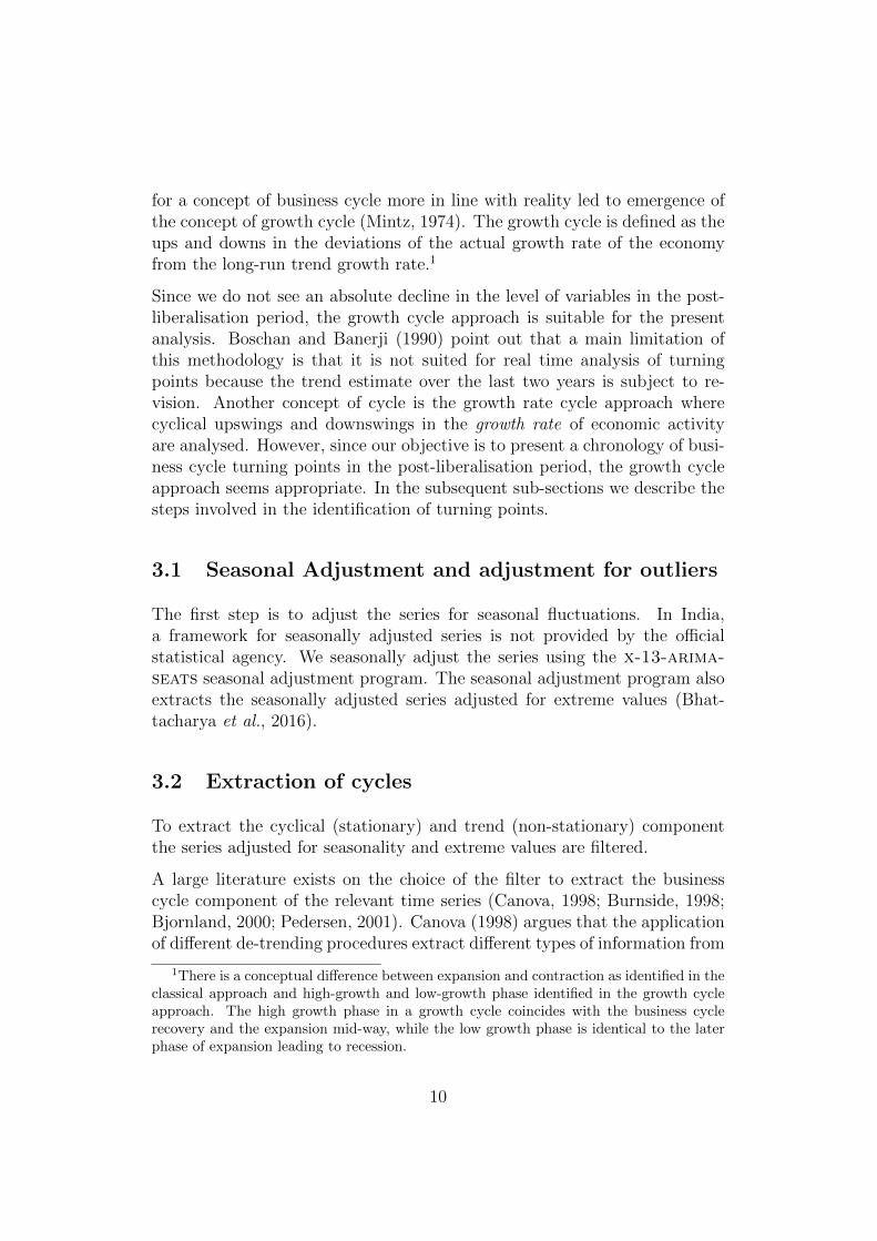
for a concept of business cycle more in line with reality led to emergence ofthe concept of growth cycle (Mintz, 1974). The growth cycle is defined as theups and downs in the deviations of the actual growth rate of the economyfrom the long-run trend growth rate.1

Since we do not see an absolute decline in the level of variables in the post-liberalisation period, the growth cycle approach is suitable for the presentanalysis. Boschan and Banerji (1990) point out that a main limitation ofthis methodology is that it is not suited for real time analysis of turningpoints because the trend estimate over the last two years is subject to re-vision. Another concept of cycle is the growth rate cycle approach wherecyclical upswings and downswings in the growth rate of economic activityare analysed. However, since our objective is to present a chronology of busi-ness cycle turning points in the post-liberalisation period, the growth cycleapproach seems appropriate. In the subsequent sub-sections we describe thesteps involved in the identification of turning points.

3.1 Seasonal Adjustment and adjustment for outliers

The first step is to adjust the series for seasonal fluctuations. In India,a framework for seasonally adjusted series is not provided by the officialstatistical agency. We seasonally adjust the series using the x-13-arima-seats seasonal adjustment program. The seasonal adjustment program alsoextracts the seasonally adjusted series adjusted for extreme values (Bhat-tacharya et al., 2016).

3.2 Extraction of cycles

To extract the cyclical (stationary) and trend (non-stationary) componentthe series adjusted for seasonality and extreme values are filtered.

A large literature exists on the choice of the filter to extract the businesscycle component of the relevant time series (Canova, 1998; Burnside, 1998;Bjornland, 2000; Pedersen, 2001). Canova (1998) argues that the applicationof different de-trending procedures extract different types of information from

1There is a conceptual difference between expansion and contraction as identified in theclassical approach and high-growth and low-growth phase identified in the growth cycleapproach. The high growth phase in a growth cycle coincides with the business cyclerecovery and the expansion mid-way, while the low growth phase is identical to the laterphase of expansion leading to recession.

10

the data. This results in business cycle properties differing widely acrossde-trending methods. However, commenting on Canova (1998), Burnside(1998) shows through spectral analysis, that the business cycle properties ofvariables are robust to the choice of the filtering methods if the definition ofbusiness cycle fluctuations are uniform across all the de-trending methods.

To derive the cyclical component, the literature on business cycles mainly re-lies on either the Hodrick-Prescott filter or the band-pass filters proposed byBaxter and King (Baxter and King, 1999) and Christiano-Fitzgerald (Chris-tiano and Fitzgerald, 2003). Band-pass filters eliminate very slow movingtrend components and very high frequency components while retaining theintermediate business cycle fluctuations.

A limitation of the commonly used Hodrick-Prescott filter is that the findingson business cycle facts are sensitive to the different values of the smoothingparameter(Bjornland, 2000). Alp et al. (2011) find that the choice of thesmoothing parameter in the HP filter has important implications for thevolatility of the trend term and average business cycle length observed in thedata.2 An inappropriate choice of this parameter may result in business cyclefacts, which are at odds with the data. Nilsson and Gyomai (2011) comparethe revision properties of different de-trending and smoothing methods (cy-cle estimation methods), including Phase-Average-Trend with smoothing, adouble Hodrick-Prescott (HP) filter and the Christiano-Fitzgerald (CF) fil-ter. The results indicate that the HP filter outperforms the CF filter in thestability of turning points but has a weaker performance in absolute numer-ical precision.3

We use the Christiano-Fitzgerald filter to isolate the trend and cyclical com-ponent. The NBER defines, business cycle as fluctuations having periodicityranging between 8 to 32 quarters. We use the NBER definition of businesscycle to extract the cyclical component. The cyclical component is standard-ised before the application of the dating algorithm. The cyclical componentis standardised by subtracting the mean of the cyclical component from itand dividing by the standard deviation of the cyclical component.

2The higher the value of smoothing parameter, the smoother the trend will be. Thetrend term is found to be smooth i.e. does not move much with actual cycles in the datawhen the smoothing parameter gets a high value, whereas it follows the data more closelywhen smoothing parameter gets a small value.

3For a detailed analysis of the detrending techniques see Appendix A.

11

3.3 Application of dating algorithm

The standardised cyclical component forms the input series for the applica-tion of the dating algorithm by Bry and Boschan (1971). The procedure wassubsequently revised and quantified in a better way by Harding and Pagan(2002). The Bry and Boschan (1971) algorithm is based on a standardisedset of rules that facilitates comparison of business cycle turning points acrosscountries, regions and time-periods. The Bry-Boschan (BB) and HardingPagan (HP) algorithms find the turning points as follows:

• The data is smoothed after outlier adjustment by constructing short-term moving averages.

• The preliminary set of turning points are selected for the smoothedseries subject to the criterion described later.

• In the next stage, turning points in the raw series is identified takingresults from smoothed series as the reference.

The identification of turning point dates is done subject to the followingrules:

• The first rule states that the peaks and troughs must alternate.

• The second step involves the identification of local minima (troughs)and local maxima (peaks) in a single time series, or in yt after a logtransformation.

• Peaks are found where ys is larger than k values of yt in both directions.

• Troughs are identified where ys is smaller than k values of yt in boththe directions.

• Bry and Boschan (1971) suggested the value of k as 5 for monthly fre-quency which Harding and Pagan (2002) transformed to 2 for quarterlyseries.

• Censoring rules are put in place for minimum duration of phase (frompeak to trough or trough to peak) and for a complete cycle (from peakto peak or from trough to trough).

• Harding and Pagan identify minimum duration of a phase to be 2 quar-ters and the minimum duration of a complete cycle to be 5 quarters.

• For monthly data, the minimum duration is 5 months and 15 monthsfor phase and cycle respectively.

12

• The identification of turning points is avoided at extreme points.

The algorithm also generates key summary statistics such as the durationand amplitude of each phase.

1. Duration: It is computed as the number of quarters from peak to troughduring a slowdown phase or from trough to the next peak in the speed-up phase.

2. Amplitude: The amplitude is calculated as the maximum drop (rise)from peak (trough) to trough (peak) during episodes of recession (ex-pansion).

The application of the Harding-Pagan dating algorithm is done using the Rpackage BCDating.4.

4 Empirical analysis

We use the quarterly GDP series (Base year 2004-05) to identify the chronol-ogy of business cycle turning points.5 This series is available from 1996Q2 (Apr-Jun) to 2014 Q3 (Jul-Sep). The series is adjusted for seasonalityand then filtered for outliers. The cyclical component is extracted using theChristiano-Fitzgerald filter using the NBER business cycle periodicity andthen standardised. The standardised cyclical component is then subject tothe rules of the dating algorithm by Harding and Pagan (2002). In additionto reporting the peak and trough dates, we also report descriptive statisticsabout the nature of cycles. These include the average duration and ampli-tude of expansion and recession and the coefficient of variation of durationand amplitude of expansion and recession. These summary statistics enableus to form judgements about the nature of business cycles.

4.1 Business cycle turning points

First, we extract the cyclical component of GDP using the NBER businesscycle periodicity of 2-8 years and then apply the dating algorithm by Harding

4https://cran.r-project.org/web/packages/BCDating/BCDating.pdf5The Central Statistical Organisation revised the GDP series with a new base year of

2011-12. The revised series is available only from 2011 Q2. Hence we stick to the serieswith the old base year for our analysis.

13

Figure 3 Turning points from 1996 to 2014

This figure shows the turning points in the cyclical component of GDP. Here the cyclicalcomponent is extracted using the CF filter using the NBER definition of business cycle

periodicity of 2 to 8 years.

2000 2005 2010

−1.

5−

0.5

0.0

0.5

1.0

1.5

2.0

GDP

Cyc

lical

com

pone

nt (

stan

dard

ised

)

and Pagan (2002). The application of dating algorithm gives us periods ofexpansion and recession along with their duration and amplitude.

Figure 3 and Table 3 shows three episodes of recession in the economy duringthe period 1996-2014. Using GDP as the reference series, the first episode ofrecession was in the period: 1999Q4 to 2003Q1, the second recession was inthe period 2007Q2 to 2009Q3, and the third recession in the period 2011Q2to 2012Q4.

Our findings are consistent with the reference chronology of turning pointsidentified by OECD for India. The OECD provides the chronology of turningpoints in the reference series for individual countries. Upto 2012, the mainreference series used was the IIP. Since 2012, GDP is used as the referenceseries for identification of turning points. They apply the growth cycle ap-proach for the identification of turning points. The first period of recessionis from 1999 December to 2003 January. This is similar to the first period ofrecession identified by us: 1999 Q4 (October-December) to 2003 Q1 (January-December). The OECD identifies the second period of recession from 2007October to 2009 March. This is again similar to our second period of reces-sion: 2007 Q2 (April-June) to 2009 (July-September). The OECD identifiesthe third period of recession from 2011 January to 2013 March. Again, this

14

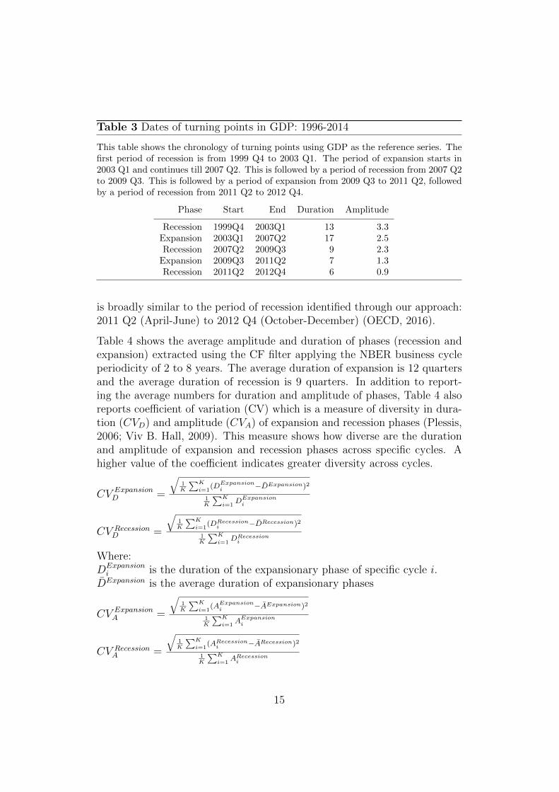
Table 3 Dates of turning points in GDP: 1996-2014

This table shows the chronology of turning points using GDP as the reference series. Thefirst period of recession is from 1999 Q4 to 2003 Q1. The period of expansion starts in2003 Q1 and continues till 2007 Q2. This is followed by a period of recession from 2007 Q2to 2009 Q3. This is followed by a period of expansion from 2009 Q3 to 2011 Q2, followedby a period of recession from 2011 Q2 to 2012 Q4.

Phase Start End Duration Amplitude

Recession 1999Q4 2003Q1 13 3.3Expansion 2003Q1 2007Q2 17 2.5Recession 2007Q2 2009Q3 9 2.3

Expansion 2009Q3 2011Q2 7 1.3Recession 2011Q2 2012Q4 6 0.9

is broadly similar to the period of recession identified through our approach:2011 Q2 (April-June) to 2012 Q4 (October-December) (OECD, 2016).

Table 4 shows the average amplitude and duration of phases (recession andexpansion) extracted using the CF filter applying the NBER business cycleperiodicity of 2 to 8 years. The average duration of expansion is 12 quartersand the average duration of recession is 9 quarters. In addition to report-ing the average numbers for duration and amplitude of phases, Table 4 alsoreports coefficient of variation (CV) which is a measure of diversity in dura-tion (CVD) and amplitude (CVA) of expansion and recession phases (Plessis,2006; Viv B. Hall, 2009). This measure shows how diverse are the durationand amplitude of expansion and recession phases across specific cycles. Ahigher value of the coefficient indicates greater diversity across cycles.

CV ExpansionD =

√1K

∑K

i=1(DExpansion

i −DExpansion)2

1K

∑K

i=1DExpansion

i

CV RecessionD =

√1K

∑K

i=1(DRecession

i −DRecession)2

1K

∑K

i=1DRecession

i

Where:DExpansioni is the duration of the expansionary phase of specific cycle i.

DExpansion is the average duration of expansionary phases

CV ExpansionA =

√1K

∑K

i=1(AExpansion

i −AExpansion)2

1K

∑K

i=1AExpansion

i

CV RecessionA =

√1K

∑K

i=1(ARecession

i −ARecession)2

1K

∑K

i=1ARecession

i

15

Table 4 Summary statistics of GDP growth cycles

This table shows the summary statistics of growth cycle turning points. It shows theaverage duration and amplitude of expansion and recessions. The average amplitude of

expansion is seen to be 2.5% while the average amplitude of recession is 2.2%. Theaverage duration of expansion is seen to be 12 quarters while the average duration ofrecession is seen to be 9.3 quarters. The table also shows the coefficient of variation

(CV) in duration and amplitude across expansions and recessions. We find that diversityin durations of expansions and recessions is similar. The diversity in duration of

expansion is seen to be 0.34 while the diversity in duration of recession is 0.31. Turningto the diversity in amplitude, we find that the amplitude of recession is more diverse at

0.45. The diversity in amplitude of expansion is 0.38. This implies that some episodes ofrecession are more severe than the others across specific cycles.

Exp/Rec Average amplitude Average duration Measure of diversity Measure of diversity(in per cent) (in quarters) in duration (CVD) in amplitude (CVA)

Expansion 2.5 12.0 0.34 0.38Recession 2.2 9.3 0.31 0.45

Where:AExpansioni is the amplitude of the expansionary phase of specific cycle i.AExpansion is the average amplitude of expansionary phases.

Table 4 shows that the diversity in duration of recessions and expansionsare similar (both are equally diverse) whereas we see greater diversity in theamplitude of recessions when compared to expansions. This implies thatsome recessions are more severe relative to the others across different cycles.

We compare our findings on average duration of phases with the findingsreported in earlier literature. The average duration of phases is found belonger than the duration reported by the earlier literature (Mohanty et al.,2003; Rand and Tarp, 2002; Dua and Banerji, 2012) (See Table 5). Mohantyet al. (2003) applies the growth cycle approach to IIP and identifies 13 growthcycles during the period 1970-71 to 2001-02. The authors find that theaverage duration of expansion is 4 quarters. Recessions are characterised byrelatively longer duration of 5 quarters. Dua and Banerji (2012) using thegrowth rate cycle approach for the period 1960-2010 find that the averageduration of speed-up is 5 quarters and average duration of slowdown is 6quarters. One plausible explanation for relatively shorter durations of phasesin earlier studies could be that these studies cover the pre-reform period. Inthe pre-reform period, the fluctuations were driven by short-lived and volatileweather and oil price shocks. Inventory-investment fluctuations which is

16

Table 5 Changing nature of Indian business cycle: Evidence from the liter-ature

This table presents a comparison of the average duration of expansion and recession re-ported in the literature. It provides evidence of change in the nature of business cycleturning points. We find that the average duration of expansion is 12 quarters and theaverage duration of recession is 9 quarters. This is in contrast to the relatively shorterduration reported in the literature ((Mohanty et al., 2003; Dua and Banerji, 2012))

Reference time period Average duration Average durationof expansion of recession

Mohanty (2003) 1970-2001 4 quarters 5 quartersDua and Banerji (2012) 1960-2010 5 quarters 6 quartersOur findings 1996-2014 12 quarters 9 quarters

Table 6 Change in U.S business cycles over time

This table reports the average duration of recession (peak to trough), expansion (troughto peak) and cycle (peak to peak and trough to trough) for the U.S over three distincttime periods. If we compare the period 1854-1919 and 1919-1945, we find that recessions(peak to trough) have become shorter and expansions have become longer in 1919-1945.Consequently the cycles have become longer in 1919-1945 as compared to 1845-1919.

Cycles Peak to Trough to Trough to Peak totrough peak trough peak

1854-1919 (16 cycles) 21.6 26.6 48.2 48.91919-1945 (6 cycles) 18.2 35.0 53.2 53.01945-2009 (11 cycles) 11.1 58.4 69.5 68.5

central to a conventional business cycle did not play a prominent role.6

4.2 Characteristics of turning points: Have the cycleschanged over time?

Do the characteristics of business cycles change over time? Table 6 showsthe changing nature of U.S business cycles over time. Comparing two dis-tinct periods–1854-1919 and 1945-2009, we find that recessions (from peakto trough) have become shorter and cycles (from trough to trough; or frompeak to peak) have become longer.

In recent decades, a number of emerging economies have undergone structuraltransformation and reforms aimed at greater market orientation. There is an

6We cannot compare the findings on coefficient of variation as to the best of our knowl-edge this statistic is not reported in earlier studies.

17

emerging strand of literature that studies the changes in business cycle factsin response to these changes (Kim et al., 2003; Alp et al., 2012; Ghate et al.,2013). A key finding of this literature is that, emerging economy cycles havechanged in the post reform period. Alp et al. (2012) compare business cycleproperties of the Turkish economy between the pre and post 2001 period.The authors find that the post 2001 period is associated with a significantdecline in the volatility of GDP, consumption and investment. In a broaderstudy Kim et al. (2003) analyse the cyclical features of seven Asian countries7

spanning the period 1960-1996. Since most of these countries experiencedstructural transformation, the authors compare the business cycle character-istics between two sub-periods (1960-1984) and (1984-1996) to understandwhether business cycle characteristics change in response to structural trans-formation and policy reforms. A key finding emerging from the analysis isthat the amplitude of economic fluctuations in Asian economies seems to bedampening over time. The decrease in amplitude of economic fluctuations isexplained by a shift in sectoral composition away from agriculture.

For India, Ghate et al. (2013) present a comparison of the business cyclestylised facts for the pre and post reform period. The authors find thatpost reform Indian business cycle stylised facts resemble that of an economyin transition. While the volatility of macroeconomic variables in the post-reform period in India is high and similar to emerging market economies, interms of correlation and persistence, the Indian business cycle looks similarto advanced economies, and less like emerging market economies.

Studies find that business cycle stylised facts change over time. In this sectionwe formally explore whether the duration of business cycle has changed overtime. This analysis cannot be performed using GDP since the quarterly seriesis available only from 1996. In order to gain intuition into the changing natureof cycles, we use IIP for which we have a longer time series. We analyse theseries in two phases: pre-reform phase from 1971-1990 and post-reform phasefrom 1992-2015. We follow the same approach. We adjust the series forseasonality and apply the CF filter to extract the cyclical component. TheNBER business cycle periodicity of 2-8 years is used to extract the cyclicalcomponent. To the standardised cyclical component of pre and post-reformIIP, we apply the dating algorithm by Bry and Boschan (1971).

Table 7 shows the average duration of expansions and recessions in the twosub-periods. Table shows that while expansions have become longer, reces-sions have become shorter in the post-reform period. As an outcome, cycles

7The authors study: Indonesia, Korea, Malaysia, The Philippines, Singapore, Taiwan,and Thailand

18

Table 7 Average duration in quarters: Evidence from pre and post IIP

This table presents a comparison of the average duration of expansion, recession andoverall cycle between the pre and post reform period. We find that the average durationof expansion has increased and the average duration of recession has reduced. As a resultthe average duration of cycle has increased.

Reference time period Average duration Average duration Average durationof expansion of recession of cycle

1971-1990 5.2 6.7 11.91992-2014 5.9 6.3 12.2

Table 8 Have the phases of cycles become more diverse over time?

Phase CVD CVA

Expansion Recession Expansion Recession1971-1990 0.28 0.32 0.61 0.591992-2014 0.43 0.46 0.74 0.71

have become longer. This analysis shows over time the duration of cycleshave changed.

Table 8 reports the coefficient of variation in duration and amplitude ofphases across different cycles in the pre and post reform period. Table showsthat in the post-reform period both expansions and recessions have becomediverse in terms of duration and amplitude. Some episodes of recession arerelatively more deeper and severe relative to others in the post-reform period.Similarly there is considerable variation in the duration of expansion and re-cession across specific cycles in the post-reform period. Some are short-livedwhile others are relatively more persistent. This dimension of change is hid-den if we limit our analysis to comparing average duration and amplitudeof phases in pre and post reform period. Our analysis points to interestingfeatures about the Indian business cycles. While the average cycle has be-come longer in the post-reform period, episodes of expansion and recessionare relatively more diverse in the post-reform period.

We present a description of the characteristics of the business cycle turningpoints in the post-reform period. Using seasonally adjusted quarterly GDPfrom 1996Q2 to 2014 Q3 we identify three episodes of recession: 1999Q4 to2003Q1, 2007Q2 to 2009Q3 and 2011Q2 to 2012Q4. The average duration ofexpansion is seen to be 12 quarters while the average duration of recession isseen to be 9.3 quarters. We also report coefficient of variation: a measure ofdiversity of amplitude and duration of expansion and recession across specificcycles. We find that while the duration of both expansion and recession areequally diverse, recessions have a more diverse amplitude as compared to

19

expansions. We offer evidence of change in the characteristics of turningpoints over time using IIP. In addition to reporting evidence of change in theaverage duration and amplitude of expansion and recession, we also showchange in the diversity of amplitude and duration of expansion and recessionover time.

5 Sensitivity of turning points chronology: Some

robustness checks

In this section we present robustness checks to examine the sensitivity of ourfindings on business cycle chronology to the choice of filter and to the choiceof the reference variable. We perform two robustness checks. First, we checkthe sensitivity of our results to the detrending procedures. To do this, weuse the Hodrick-Prescott filter in place of the CF filter to extract the cyclicalcomponent. We perform this check to test if cyclical components derivedfrom different detrending procedures yield similar turning points. Second,we check the robustness of our findings to the choice of reference series. Weuse IIP, non-agricultural, non Government GDP and firms’ net sales index asa proxy for analysing business cycle chronology to test the if the chronologyof turning points are sensitive to the choice of the reference series.

5.1 Robustness check I: Using Hodrick-Prescott filter

In this section we report the sensitivity of our findings to the choice of filterto detrend the series. Figure 4 and Table 9 shows the turning points in thecyclical component of GDP extracted using the HP filter. As discussed earlierthe choice of the smoothing parameter is crucial for the application of the H-P filter. With quarterly data, the smoothing parameter is set priori to 1600.With this value of smoothing parameter, the H-P filter defines the cyclicalcomponent as fluctuations with a period less than 8 years. H-P filter witha smoothing parameter of 1600 is comparable to a CF filter which extractscycles of periodicity ranging between 2-8 years. This enables comparison ofcycles extracted through both the filters.

It is noteworthy that broadly similar periods of recession (2000 Q1–2003 Q1,2007 Q4–2008 Q4 and 2011 Q1–2014 Q1) are identified using the cyclicalcomponent extracted through the Hodrick-Prescott filter. A comparison ofTable 3 and Table 9 shows that the application of HP filter to extract cyclical

20

Figure 4 Turning points from 1996 to 2014 using HP filter

This figure shows the turning points in the cyclical component of GDP. Here the cyclicalcomponent is extracted using the HP filter using the conventional smoothing parameter

of 1600.

2000 2005 2010

−2

−1

01

2

GDP

Cyc

lical

com

pone

nt (

stan

dard

ised

)

Table 9 Dates of turning points in GDP using HP filter: 1999-2014

This table shows the business cycle chronology using HP filter. Broadly similar periods ofrecession (2000 Q1–2003 Q1, 2007 Q4–2008 Q4 and 2011 Q1–2014 Q1) are identified usingthe cyclical component extracted through the HP filter. In addition, some high frequencycycles are also extracted through the application of the HP filter.

Phase Start End Duration Amplitude

Recession 2000Q1 2003Q1 12 4.3Expansion 2003Q1 2004Q1 4 0.9Recession 2004Q1 2004Q4 3 0.1

Expansion 2004Q4 2007Q4 12 2.7Recession 2007Q4 2008Q4 4 2.1

Expansion 2008Q4 2009Q3 3 1.6Recession 2009Q3 2010Q1 2 1.5

Expansion 2010Q1 2011Q1 4 2.0Recession 2011Q1 2014Q1 12 2.9

21

component yields more number of cycles. This is attributed to the propertyof HP filter. The reason is that the HP filter puts weight on high frequencieswhereas the two band pass filters do not put any weight on these frequen-cies. As an outcome some high frequency cycles are also extracted throughthe application of HP filter. A visual inspection of the cyclical componentextracted through the CF and HP filter also shows that the CF filter extractssmoother cycles compared to the HP (See Figures 3 and 4).

5.2 Robustness check II: Growth cycle chronology us-ing other reference series

We turn to examine the turning points using some additional series that couldbe considered as proxy indicators to study the business cycle chronology. Weuse IIP, GDP excluding agriculture and government and Firms’ net salesindex as reference series to analyse the business chronology. We excludeagriculture since agriculture is affected by strong seasonal fluctuations whichdepend on the outcome of the monsoon. In contrast, the government sectoris affected by significant short run volatility due to the dynamics of publicsector outlays. GDP excluding agriculture and excluding government focuseson the output of individuals, small firms and large firms and is closely relatedto business cycles.

Next, we use a measure of output utilising firm data. We construct an in-dex of firms net sales. For the construction of the firms’ net sales indexwe focus on all listed firms observed in the CMIE Prowess database otherthan finance and oil companies. We exclude finance companies since theyfollow very different accounting concepts. We also exclude oil companiessince their balance-sheets experience large changes owing to government’sdecisions about administered prices. These fluctuations are not an indica-tion of underlying business cycle conditions. For the rest of the firms weconstruct an index of their net sales. This is done as follows: For each pair ofquarters, we construct a panel of firms observed in both quarters, and workout the percentage change in the sum of net sales across all the firms. Thesepercentage changes are used to construct a net sales index.8

Following our baseline methodology we use the CF filter to extract the cycli-cal component and then apply the Bry-Boschan algorithm. Tables 10, 11

8For details on the methodology to construct netsales index see http://ajayshahblog.blogspot.in/2013/07/

a-better-output-proxy-for-indian-economy.html

22

Table 10 Dates of turning points in IIP: 1999-2014

This table shows the business cycle chronology using IIP as the reference series. Theperiods of recession: 2000 Q2 to 2003 Q3, 2007 Q4 to 2009 Q2 and 2011 Q1 to 2013 Q4are broadly similar to the three periods of recession identified using GDP as the referenceseries.

Phase Start End Duration Amplitude

Recession 2000Q2 2003Q3 13 2.2Expansion 2003Q3 2004Q4 5 1.3Recession 2004Q4 2006Q1 5 1.5

Expansion 2006Q1 2007Q4 7 3.8Recession 2007Q4 2009Q2 6 5.3

Expansion 2009Q2 2011Q1 7 3.5Recession 2011Q1 2013Q4 11 1.6

and 12 show the phases of expansion and recession in IIP, GDP excludingagriculture and excluding government and Firms’ net sales respectively. Theperiods of recession identified using the three series are broadly in conformitywith the periods of recession identified in the GDP series. IIP as a referenceseries yields 2000 Q2 to 2003 Q3, 2007 Q4 to 2009 Q2 and 2011 Q1 to 2013Q4 as periods of recession. These are broadly similar to the three periodsof recession identified using GDP as the reference series. GDP excludingagriculture and government yields the three periods of recession: 2000 Q1to 2003 Q1, 2007 Q2 to 2009 Q3 and 2011 Q2 to 2012 Q4. These are al-most identical to the recessions identified using GDP as the reference series.Firms net sales index yields 2000 Q2-2002 Q4, 2007 Q4- 2009 Q3 and 2011Q2 to 2013 Q4. These are broadly in conformity with the recession periodsidentified using GDP as the reference series.9

On the whole, the robustness checks show that the chronology of recession isbroadly robust to the choice of the detrending procedure and to the choiceof the reference series.

6 Description of recessions and expansions

Figure 5 shows the performance of key macroeconomic variables during thethree identified periods of recession. The shaded portions show the period of

9In addition to the three common recession periods, an additional short period ofrecession is identified in each of the three series in the period ranging from mid 2004 toearly 2006.

23

Table 11 Dates of turning points in GDP (excluding agriculture and Gov-ernment.) 1996-2014

This table shows the chronology of business cycle turning points using GDP excludingagriculture and Government as the reference series. The periods of recession: 2000 Q1to 2003 Q1, 2007 Q2 to 2009 Q3 and 2011 Q2 to 2012 Q4 are almost identical to therecessions identified using GDP as the reference series.

Phase Start End Duration Amplitude

Recession 2000Q1 2003Q1 12 2.7Expansion 2003Q1 2004Q2 5 0.6Recession 2004Q2 2005Q1 3 0.2

Expansion 2005Q1 2007Q2 9 2.2Recession 2007Q2 2009Q3 9 3.3

Expansion 2009Q3 2011Q2 7 1.8Recession 2011Q2 2012Q4 6 0.7

Table 12 Dates of turning points in Firms’ net sales: 1999-2014

This table shows the chronology of business cycle turning points using firms’ net sales asthe reference series. The periods of recession 2000 Q2 to 2002 Q4, 2007 Q4 to 2009 Q3and 2011 Q2 to 2013 Q4 are broadly in conformity with the recession periods identifiedusing GDP.

Phase Start End Duration Amplitude

Recession 2000Q2 2002Q4 10 2.7Expansion 2002Q4 2004Q3 7 1.9Recession 2004Q3 2005Q4 5 0.9

Expansion 2005Q4 2007Q4 8 1.2Recession 2007Q4 2009Q3 7 3.2

Expansion 2009Q3 2011Q2 7 3.8Recession 2011Q2 2013Q4 10 3.1

24

Figure 5 Slowdown in macro-economic variables during the identified peri-ods of recession

This figure shows the growth patterns in key macro-economic variables during the iden-tified periods of recession. The figure shows that the year-on-year growth in GDP, IIP,non-food credit and investment shows considerable decline during the shaded periods ofrecession.

GDP growth IIP growth

2000 2005 2010 2015

24

68

102

46

810

Y−

o−Y

Cha

nge

(Per

cen

t)

2000 2005 2010 2015

−5

05

1015

−5

05

1015

Y−

o−Y

Cha

nge

(Per

cen

t)

Credit growth Investment growth

2000 2005 2010 2015

510

2030

405

1020

3040

Y−

o−Y

Cha

nge

(Per

cen

t)

2000 2005 2010

510

2030

510

2030

Y−

o−Y

Cha

nge

(Per

cen

t)

25

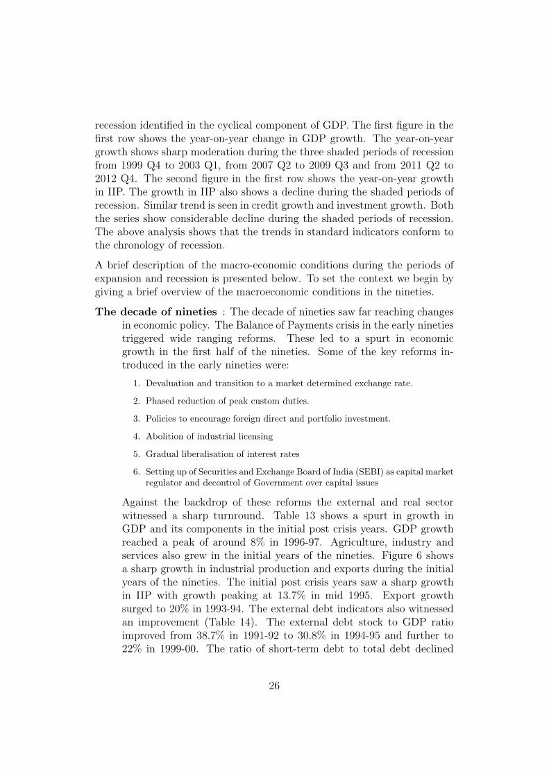
recession identified in the cyclical component of GDP. The first figure in thefirst row shows the year-on-year change in GDP growth. The year-on-yeargrowth shows sharp moderation during the three shaded periods of recessionfrom 1999 Q4 to 2003 Q1, from 2007 Q2 to 2009 Q3 and from 2011 Q2 to2012 Q4. The second figure in the first row shows the year-on-year growthin IIP. The growth in IIP also shows a decline during the shaded periods ofrecession. Similar trend is seen in credit growth and investment growth. Boththe series show considerable decline during the shaded periods of recession.The above analysis shows that the trends in standard indicators conform tothe chronology of recession.

A brief description of the macro-economic conditions during the periods ofexpansion and recession is presented below. To set the context we begin bygiving a brief overview of the macroeconomic conditions in the nineties.

The decade of nineties : The decade of nineties saw far reaching changesin economic policy. The Balance of Payments crisis in the early ninetiestriggered wide ranging reforms. These led to a spurt in economicgrowth in the first half of the nineties. Some of the key reforms in-troduced in the early nineties were:

1. Devaluation and transition to a market determined exchange rate.

2. Phased reduction of peak custom duties.

3. Policies to encourage foreign direct and portfolio investment.

4. Abolition of industrial licensing

5. Gradual liberalisation of interest rates

6. Setting up of Securities and Exchange Board of India (SEBI) as capital marketregulator and decontrol of Government over capital issues

Against the backdrop of these reforms the external and real sectorwitnessed a sharp turnround. Table 13 shows a spurt in growth inGDP and its components in the initial post crisis years. GDP growthreached a peak of around 8% in 1996-97. Agriculture, industry andservices also grew in the initial years of the nineties. Figure 6 showsa sharp growth in industrial production and exports during the initialyears of the nineties. The initial post crisis years saw a sharp growthin IIP with growth peaking at 13.7% in mid 1995. Export growthsurged to 20% in 1993-94. The external debt indicators also witnessedan improvement (Table 14). The external debt stock to GDP ratioimproved from 38.7% in 1991-92 to 30.8% in 1994-95 and further to22% in 1999-00. The ratio of short-term debt to total debt declined

26

Table 13 Growth rate in GDP and its sectors

This table shows the growth rate in GDP and its sectors in the nineties. The table showsa pick-up in growth rate during the initial post-crisis years from 1992-1996. Since 1997 abroad-based moderation is seen in growth rates for overall GDP, agriculture and industrialGDP. GDP growth surged from 1.36% in 1991-92 to 7.97% in 1996-97 before slowing downin 1997-98. The growth in GDP (Industry) reached its peak at 11.29% in 1995-96 beforeslowing down in subsequent years. GDP (Agriculture) also slowed down in the second halfof nineties.

Year GDP Agriculture Industry Services

1991-92 1.43 -1.95 0.34 4.691992-93 5.36 6.65 3.22 5.691993-94 5.68 3.32 5.5 7.381994-95 6.39 4.72 9.16 5.841995-96 7.29 -0.7 11.29 10.111996-97 7.97 9.92 6.39 7.531997-98 4.3 -2.55 4.01 8.931998-99 6.68 6.32 4.15 8.281999-00 7.59 2.67 5.96 11.19

from 8.3% in 1991-92 to 4.3% in 1994-95 to 4% in 1999-00. Ratioof foreign exchange reserves to total debt and the ratio of short-termdebt to foreign exchange reserves also witness an improvement in thenineties.

Aggregate savings and investments were also buoyant during the firsthalf of the nineties. Gross domestic savings as a percent to GDP rosefrom 21.3 in 1991-92 to 24.15% in 1997-98. Similarly gross domesticcapital formation rose from 22.5% in 1991-92 to reach a peak of 26.1%in 1995-96 before slowing down to 22% in 1996-97.

From 1997 onwards we see a deceleration in India’s growth story (Acharya,2012). GDP growth moderated to 4.3% in 1997-98 from 8% in 1996-97.Agriculture and industrial growth also slowed down in 1997-98. Thegrowth in manufacturing fell sharply to less than 1% in 1997-98 from9.5% in the previous year. Figure ?? shows a slump in industrial pro-duction and exports in 1997. The moderation in growth from 1997-98onwards could be attributed to the investment boom of the previousyears. The investment boom of the previous three years had built uplarge capacities, which discouraged further expansion. Another reasoncould be the advent of coalition governance had dampened businessconfidence.

The subsequent paragraphs present an overview of the phases of ex-

27

Figure 6 Industrial production and exports in the nineties

This figure shows the year-on-year growth in industrial production and exports in thenineties. The first figure shows the growth in IIP and the second figure captures thegrowth in exports. The growth in both these variables witnessed a surge in the initialyears of the nineties before moderating from 1996-97 onwards.

1993 1994 1995 1996 1997 1998 1999

05

10

YoY

Cha

nge

(Per

cen

t)

1993 1994 1995 1996 1997 1998 1999

−10

010

20

YoY

Cha

nge

(Per

cen

t)

Table 14 External debt indicators in the nineties

This table shows the key external debt indicators in the nineties. One of the outcome ofthe reform measures introduced in the nineties was the improvement in the external debtindicators. The stock of external debt to GDP improved from 38.7% in 1991-92 to 22% in1999-2000. Improvements are visible in other indicators of external debt such as ratio ofshort-term debt to total debt, ratio of foreign exchange reserves to total debt and ratio ofshort-term debt to foreign exchange reserves.

Year External debt to GDP (%) Ratio of short-term debt debt Ratio of foreign exchange reserves Ratio of short-term debtto total debt to total debt to foreign exchange reserves

1991-92 38.7 8.3 10.8 76.71992-93 37.5 7.0 10.9 64.51993-94 33.8 3.9 20.8 18.81994-95 30.8 4.3 25.4 16.91995-96 27.0 5.4 23.1 23.21996-97 24.6 7.2 28.3 25.51997-98 24.3 5.4 31.4 17.21998-99 23.6 4.4 33.5 13.21999-00 22.0 4.0 38.7 10.3Source: India’s external debt: A status report 2014-15

28

Table 15 Key macro-economic conditions in 2000-03

This table shows the growth rate in GDP, gross fixed investment as a ratio to GDP andsavings as a ratio to GDP during 2000-03 period. We see a moderation in GDP growthrate. Broadly, the savings rate exceeded the investment rate in this period.

1999-2000 2000-01 2001-02 2002-03

Annual GDP growth rate 7.6 4.3 5.5 4.0Gross fixed investment (% to GDP) 24.1 22.8 25.1 23.7Savings (% to GDP) 25.7 23.8 24.9 25.93

pansion and recession from 1999 onwards.

End 1999 to 2003Q1 recession : Table 15 shows the performance of keymacro-economic indicators during the period 2000-03. GDP growthslowed down from 7.6% in 1999-2000 to 4.3% in 2000-01. The ratioof gross fixed investment to GDP was lower than the ratio of savingsto GDP. With low private investment demand, foreign investment wassought to improve the investment climate. However in the aftermathof the Asian financial crisis, FDI inflows did not gain momentum. Thebursting of the dot-com bubble, and the brief decline in software exportgrowth after the “Y2K” problem also contributed to the slowdown (Na-garaj, 2013). On the whole, the macro-economic conditions were largelybenign. But conditions began to look positive from 2003 onwards. Theupswing from 2003 onwards was driven by a boom in investment anda revival of foreign capital inflows that had dried up after the Asianfinancial crisis.

2003-mid2007 expansion : The economy witnessed an upswing in thecycle, primarily led by high credit growth during this period whenfirms borrowed and initiated a number of projects. What triggeredthis boom? From 2001 to 2004, RBI engaged in sterilised interven-tion. In early 2004, it ran out of bonds. This period was marked bycurrency trading that was not backed by sterilisation. Without steril-isation dollar purchases resulted in injection of rupee in the economy.The economy became flush with funds, interest rates went down. Thiskicked off a bank credit boom from 2004 to 2007. The third graph ofFigure 5 shows a surge in credit growth between 2004 to 2007. Thecredit growth reached a peak of 40% during this period. GDP growthremained strong at 8-10% during this period.

Mid 2007 to mid 2009 recession : Global financial crisis affected Indiathrough trade and financial linkages. Export growth saw a sharp de-

29

Figure 7 Slowdown in investment and exports in 2008-09

This figure shows the slowdown in investment and exports growth during the 2008-09period. The first growth the year-on-year growth in investment and the second graphshows the year-on-year growth in exports.

510

1520

2530

Per

cen

t

1996 2000 2004 2008 2011 2015

−20

020

4060

Per

cen

t2000 Q1 2003 Q1 2006 Q2 2009 Q3 2012 Q3 2015 Q4

celeration in this period (Patnaik and Shah, 2010; Patnaik and Pundit,2014). This could have been the result of greater synchronisation of do-mestic cycles with global cycles (Jayaram et al., 2009). The immediatetransmission of the financial crisis to India was through a slowdown ofcredit flows which was reflected in the spiking of overnight call moneyrates that rose to nearly 20 per cent in October and early November2008. Investment growth also slowed down in 2008-09 (See the firstgraph of Figure 7).

Mid 2009 to mid 2011 expansion : We saw a business cycle upswing in2009. GDP growth recovered to 8.6% in 2009-10 from 6.72% in 2008-09. The growth further strengthened to 8.9% in 2010-11. The upswingwas an outcome of a coordinated monetary and fiscal policy stimuluspackage announced in 2008-09. For example, the government intro-duced fiscal stimulus in the form of tax cuts and increased expenditureto boost consumer demand and production in key sectors. The FiscalResponsibility and Budget Management (FRBM) Act, 2003, accord-ing to which, the government is required to follow fiscal prudence toreduce its deficits to a target rate, was suspended in 2009 in order toaccommodate the stimulus policies. On the monetary side, the ReserveBank of India introduced measures, such as rate cuts, to boost liquidityand ease credit in order to boost investment. The rate cut cycle beganin October 2008 and continued till March 2010. Guidelines for Exter-nal Commercial Borrowing were also liberalised to ease firms’ access toexternal finance (Patnaik and Pundit, 2014).

Mid 2011 to 2012 recession : Since 2011, again, we saw a business cycle

30

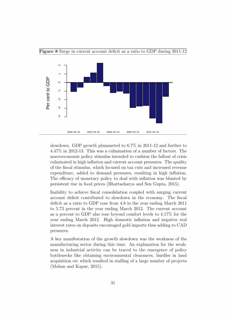
Figure 8 Surge in current account deficit as a ratio to GDP during 2011-12

2000−03−31 2003−03−31 2006−03−31 2009−03−31 2012−03−31

Per

cen

t to

GD

P

−4

−3

−2

−1

01

2

slowdown. GDP growth plummeted to 6.7% in 2011-12 and further to4.47% in 2012-13. This was a culmination of a number of factors. Themacroeconomic policy stimulus intended to cushion the fallout of crisisculminated in high inflation and current account pressures. The qualityof the fiscal stimulus, which focused on tax cuts and increased revenueexpenditure, added to demand pressures, resulting in high inflation.The efficacy of monetary policy to deal with inflation was blunted bypersistent rise in food prices (Bhattacharya and Sen Gupta, 2015).

Inability to achieve fiscal consolidation coupled with surging currentaccount deficit contributed to slowdown in the economy. The fiscaldeficit as a ratio to GDP rose from 4.8 in the year ending March 2011to 5.73 percent in the year ending March 2012. The current accountas a percent to GDP also rose beyond comfort levels to 4.17% for theyear ending March 2012. High domestic inflation and negative realinterest rates on deposits encouraged gold imports thus adding to CADpressures.

A key manifestation of the growth slowdown was the weakness of themanufacturing sector during this time. An explanation for the weak-ness in industrial activity can be traced to the emergence of policybottlenecks like obtaining environmental clearances, hurdles in landacquisition etc which resulted in stalling of a large number of projects(Mohan and Kapur, 2015).

31

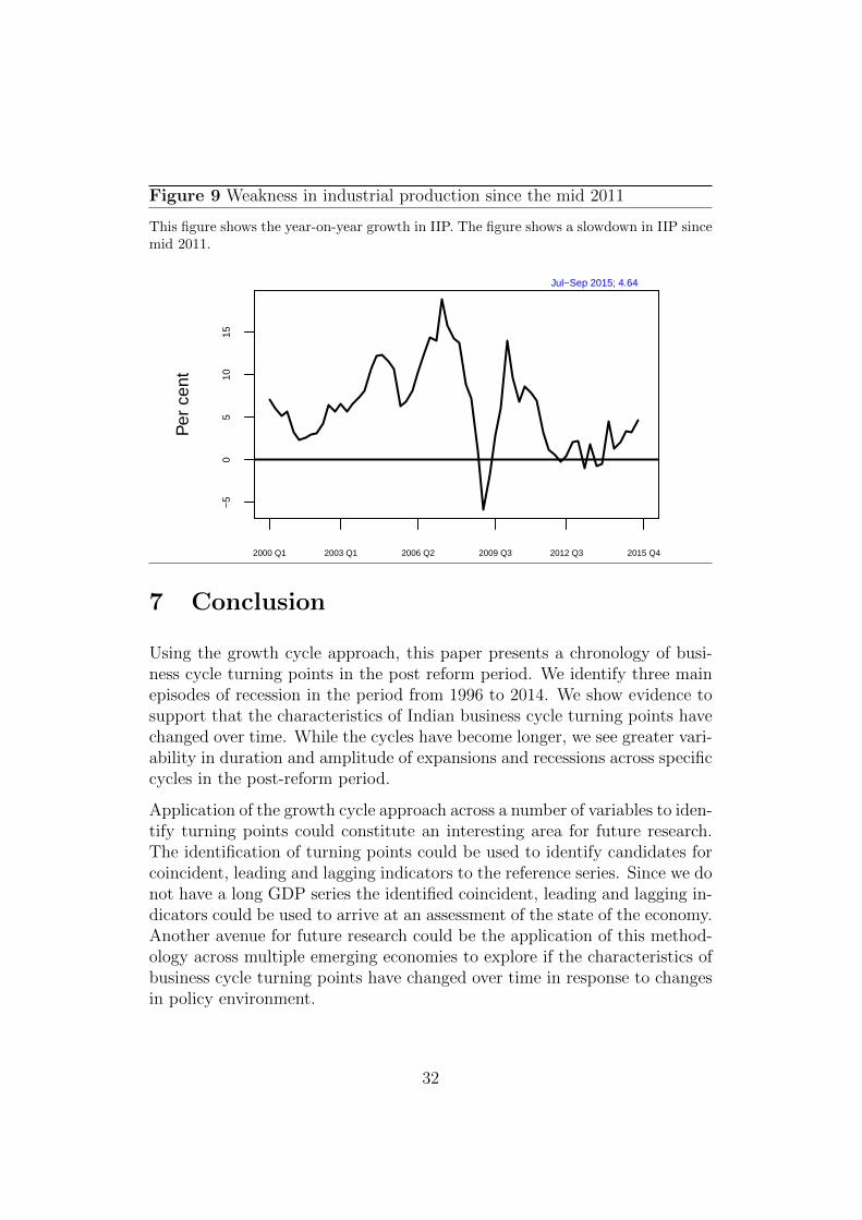
Figure 9 Weakness in industrial production since the mid 2011

This figure shows the year-on-year growth in IIP. The figure shows a slowdown in IIP sincemid 2011.

−5

05

1015

Per

cen

t

2000 Q1 2003 Q1 2006 Q2 2009 Q3 2012 Q3 2015 Q4

Jul−Sep 2015; 4.64

7 Conclusion

Using the growth cycle approach, this paper presents a chronology of busi-ness cycle turning points in the post reform period. We identify three mainepisodes of recession in the period from 1996 to 2014. We show evidence tosupport that the characteristics of Indian business cycle turning points havechanged over time. While the cycles have become longer, we see greater vari-ability in duration and amplitude of expansions and recessions across specificcycles in the post-reform period.

Application of the growth cycle approach across a number of variables to iden-tify turning points could constitute an interesting area for future research.The identification of turning points could be used to identify candidates forcoincident, leading and lagging indicators to the reference series. Since we donot have a long GDP series the identified coincident, leading and lagging in-dicators could be used to arrive at an assessment of the state of the economy.Another avenue for future research could be the application of this method-ology across multiple emerging economies to explore if the characteristics ofbusiness cycle turning points have changed over time in response to changesin policy environment.

32

A Detrending techniques

Cycle extraction is a crucial step in the growth cycle approach. Instead ofobserving the series in the time domain, it is useful to translate the seriesin a frequency domain framework. In the frequency domain, we can treatthe series as a construction of sine waves of different wave length. The trendpart of the series is comprised by the low frequency (high wave length) sinewaves, whereas the noise is formed by a set of high frequency sine waves (?).

Once we have the series in the frequency domain, we can single out the cycleswe are interested in, and eliminate the components whose wave length is toolong (trend) or too short (noise). The category of band-pass filters helpin extracting cycles of a chosen frequency (Christiano and Fitzgerald, 2003;Baxter and King, 1999). The de-trending methods need to be aligned withthe chosen business cycle frequency or periodicity.

Hodrick-Prescott filter:

yt = τt + ct

minτt∑t(yt − τt)

2 + λ ∗ sumt(τt+1 − 2 ∗ τt + τt−1)2

The initial yt series is decomposed into λt the trend component and ct -the cyclical component, with the objective being to minimise the distancebetween the trend and the original series and, at the same time to minimisethe curvature of the trend series. The trade-off between the two goals iscaptured by the λ parameter.

It is possible to transform the Hodrick-Prescott filter into frequency domain.The literature uses 1600 as the value of λ for quarterly series but it is possibleto align the λ parameter with the goal of filtering out cycles in a certainfrequency range depending upon our definition of business cycle with thehelp of the transformation into the frequency domain (Pedersen, 2001).

33

References

Acharya S (2012). “India: Crisis, reforms and growth in the nineties.” WorkingPapers 139, Stanford Center for International Development. URL https://

ideas.repec.org/p/npf/wpaper/16-160.html.

Aguiar M, Gopinath G (2004). “Emerging Market Business Cycles: The Cycleis the Trend.” NBER Working Papers 10734, National Bureau of EconomicResearch, Inc. URL http://ideas.repec.org/p/nbr/nberwo/10734.html.

Alp H, Baskaya Y, Kilinc M, Yuksel C (2011). “Estimating Optimal Hodrick-Prescott Filter Smoothing Parameter for Turkey.” Iktisat Isletme ve Finans,26(306), 09–23. URL http://EconPapers.repec.org/RePEc:iif:iifjrn:v:

26:y:2011:i:306:p:09-23.

Alp H, Baskaya YS, Kilinc M, Yuksel C (2012). “Stylized Facts for Business Cyclesin Turkey.” Working Papers 1202, Research and Monetary Policy Department,Central Bank of the Republic of Turkey. URL https://ideas.repec.org/p/

tcb/wpaper/1202.html.

Baxter M, King R (1999). “Measuring business cycles: approximate band-passfilters for economic time series.” Review of Economics and Statistics, 81(4),575–593. ISSN 0034-6535.

Bhattacharya R, Pandey R, Patnaik I, Shah A (2016). “Seasonal adjustment ofIndian macroeconomic time-series.” Working Papers 16/160, National Instituteof Public Finance and Policy. URL https://ideas.repec.org/p/npf/wpaper/

16-160.html.

Bhattacharya R, Sen Gupta A (2015). “Food Inflation in India: Causes andConsequences.” Working Papers 15/151, National Institute of Public Financeand Policy. URL https://ideas.repec.org/p/npf/wpaper/15-151.html.

Bjornland H (2000). “Detrending methods and stylized facts of business cycles inNorway- an international comparison.” Empirical Economics.

Board TC (2000). Business Cycle Indicators Handbook. The Conference Board,USA.

Boschan C, Banerji A (1990). “A reassessment of composite indexes.” In“Analysing business cycles,” M.E Sharpe, New York.

Bry G, Boschan C (1971). Cyclical Analysis of Time Series: Selected Proceduresand Computer Programs. National Bureau of Economic Research. URL http:

//www.nber.org/chapters/c2145.

Burns A, Mitchell W (1938). “Statistical indicators of cyclical revivals.” NBERBulletin, 69.

34

Burns AF, Mitchell WC (1946). Measuring Business Cycles. National Bureau ofEconomic Research.

Burnside C (1998). “Detrending and business cycle facts: A comment.” Journalof Monetary Economics.

Calderon C, Fuentes R (2006). “Characterising business cycle fluctuations inemerging economies.” Central bank of Chile working papers.

Canova F (1998). “Detrending and business cycle facts.” Journal of MonetaryEconomics.

Chitre V (1982). Growth Cycles in the Indian Economy. Artha vijnana reprint se-ries. Gokhale Institute of Politics & Economics. URL https://books.google.

co.in/books?id=o-SwAAAAIAAJ.

Chitre V (2001). “Indicators of Business Recessions and Revivals in India: 1951-1982.” Indian Economic Review, 36(1), 79–105. URL http://ideas.repec.

org/a/dse/indecr/v36y2001i1p79-105.html.

Chitre VS (2004). “Indicators of business recessions and revivals in India 1951 -82.”

Christiano L, Fitzgerald T (2003). “The band pass filter.” V International Eco-nomic Review, 44(2), 435–465.

Christoffersen PF (2000). “Dating the Turning Points of Nordic Business Cycles.”EPRU Working Paper Series 00-13, Economic Policy Research Unit (EPRU),University of Copenhagen. Department of Economics. URL https://ideas.

repec.org/p/kud/epruwp/00-13.html.

Dua P, Banerji A (1999). “An Index of Coincident Economic Indicators for theIndian Economy.” Journal of Quantitative Economics, 15, 177–201.

Dua P, Banerji A (2000). “An Index of Coincident Economic Indicators for theIndian Economy.” Working papers 73, Centre for Development Economics, DelhiSchool of Economics. URL http://ideas.repec.org/p/cde/cdewps/73.html.

Dua P, Banerji A (2001a). “An Indicator Approach to Business and Growth RateCycles: The Case of India.” Indian Economic Review, 36(1), 55–78. URLhttp://ideas.repec.org/a/dse/indecr/v36y2001i1p55-78.html.

Dua P, Banerji A (2001b). “A Leading Index for the Indian Economy.” Workingpapers 90, Centre for Development Economics, Delhi School of Economics. URLhttp://ideas.repec.org/p/cde/cdewps/90.html.

Dua P, Banerji A (2007). “Business Cycles in India.” Working Papers.

Dua P, Banerji A (2012). “Business And Growth Rate Cycles In India.” Working

35

papers 210, Centre for Development Economics, Delhi School of Economics.URL https://ideas.repec.org/p/cde/cdewps/210.html.

Dua P, Kumawat L (2005). “Modelling and Forecasting Seasonality in IndianMacroeconomic Time Series.” Working papers 136, Centre for DevelopmentEconomics, Delhi School of Economics. URL http://ideas.repec.org/p/cde/

cdewps/136.html.

Dubois E, Michaux E (2008). “Grocer 1.3: An Econometrics toolbox for Scilab.”URL http://dubois.ensae.net/grocer.html.

Gavin M, Perotti R (1997). “Fiscal Policy in Latin America.” In “NBER Macroeco-nomics Annual 1997, Volume 12,” NBER Chapters, pp. 11–72. National Bureauof Economic Research, Inc. URL https://ideas.repec.org/h/nbr/nberch/

11036.html.

Ghate C, Pandey R, Patnaik I (2013). “Has India emerged? Business cycle styl-ized facts from a transitioning economy.” Structural Change and EconomicDynamics, 24(C), 157–172. URL https://ideas.repec.org/a/eee/streco/

v24y2013icp157-172.html.

Harding D, Pagan A (1999). “Knowing the Cycle.” Melbourne Institute WorkingPaper Series wp1999n12, Melbourne Institute of Applied Economic and SocialResearch, The University of Melbourne. URL http://ideas.repec.org/p/

iae/iaewps/wp1999n12.html.

Harding D, Pagan A (2002). “Dissecting the cycle: a methodological investigation*1.” Journal of monetary economics, 49(2), 365–381. ISSN 0304-3932.

Harding D, Pagan A (2003). “A comparison of two business cycle dating methods.”Journal of Economic Dynamics and Control, 27(9), 1681–1690. URL http:

//ideas.repec.org/a/eee/dyncon/v27y2003i9p1681-1690.html.

Harding D, Pagan A (2006). “Synchronization of cycles.” Journal of Econo-metrics, 132(1), 59–79. URL http://ideas.repec.org/a/eee/econom/

v132y2006i1p59-79.html.

Harvey AC, Jaeger A (1993). “Detrending, Stylized Facts and the Business Cycle.”Journal of Applied Econometrics, 8(3), 231–47. URL http://ideas.repec.

org/a/jae/japmet/v8y1993i3p231-47.html.

Hodrick RJ, Prescott EC (1997). “Postwar U.S. Business Cycles: An EmpiricalInvestigation.” Journal of Money, Credit and Banking, 29(1), 1–16. URL http:

//ideas.repec.org/a/mcb/jmoncb/v29y1997i1p1-16.html.

Ilzetzki E, Vegh CA (2008). “Procyclical Fiscal Policy in Developing Countries:Truth or Fiction?” NBER Working Papers 14191, National Bureau of EconomicResearch, Inc. URL https://ideas.repec.org/p/nbr/nberwo/14191.html.

36

Jayaram S, Patnaik I, Shah A (2009). “Examining the Decoupling Hypothesisfor India.” Economic and Political Weekly, 44(44), 109–116. ISSN 00129976,23498846. URL http://www.jstor.org/stable/25663740.

Joshi H (1997). “Growth cycles in India : an empirical investigation.”

Kaminsky GL, Reinhart CM, Vegh CA (2004). “When it Rains, it Pours: Procycli-cal Capital Flows and Macroeconomic Policies.” NBER Working Papers 10780,National Bureau of Economic Research, Inc. URL https://ideas.repec.org/

p/nbr/nberwo/10780.html.

Kim SH, Kose MA, Plummer MG (2003). “Dynamics of Business Cycles in Asia:Differences and Similarities.” Review of Development Economics, 7(3), 462–477.URL https://ideas.repec.org/a/bla/rdevec/v7y2003i3p462-477.html.

Klein PA, Moore GH (1985). “Developing Growth Cycle Chronologies for Market-Oriented Countries.” In “Monitoring Growth Cycles in Market-Oriented Coun-tries: Developing and Using International Economic Indicators,” NBER Chap-ters, pp. 29–69. National Bureau of Economic Research, Inc. URL https:

//ideas.repec.org/h/nbr/nberch/4165.html.

Layton AP, Banerji A (2001). “Dating the Indian Business Cycle: Is OutputAll That Counts?” Indian Economic Review, 36(1), 231–240. URL http:

//ideas.repec.org/a/dse/indecr/v36y2001i1p231-240.html.

Mall O (1999). “Composite Index of Leading Indicators for Business Cycles inIndia.” RBI Occasional Papers, 20(3), 373– 414.

Mintz I (1974). “Dating United States Growth Cycle.” Technical report, NBER.

Mohan R, Kapur M (2015). “Pressing the Indian Growth Accelerator: PolicyImperatives.” IMF Working Papers 15/53, International Monetary Fund. URLhttps://ideas.repec.org/p/imf/imfwpa/15-53.html.

Mohanty J, Singh B, Jain R (2003). “Business cycles and leading indicators of in-dustrial activity in India.” Mpra paper, University Library of Munich, Germany.URL http://EconPapers.repec.org/RePEc:pra:mprapa:12149.

Nagaraj R (2013). “India’s Dream Run, 2003-08.” Economic and Political Weekly,48(20).

Nandi A (2010). “India’s cosine curve: A business cycle approach of analysinggrowth, 2007 onwards.” Corporate Economic Cell, Aditya Birla ManagementCorporation.

Nilsson R, Gyomai G (2011). “Cycle Extraction: A Comparison of the Phase-Average Trend Method, the Hodrick-Prescott and Christiano-Fitzgerald Fil-ters.” OECD Statistics Working Papers 2011/4, OECD Publishing. URLhttps://ideas.repec.org/p/oec/stdaaa/2011-4-en.html.

37

OECD (2016). “OECD Composite Leading Indicators: TurningPoints of Reference Series and Component Series.” Technical re-port, OECD. URL http://www.oecd.org/std/leading-indicators/

CLI-components-and-turning-points.pdf.

Panagariya A (2008). India: The emerging giant. Oxford University Press.

Patnaik I, Pundit M (2014). “Is India’s Long-Term Trend Growth Declining?”ADB Economics Working Paper Series 424, Asian Development Bank. URLhttp://EconPapers.repec.org/RePEc:ris:adbewp:0424.

Patnaik I, Shah A (2010). “Why India choked when Lehman broke.” FinanceWorking Papers 22974, East Asian Bureau of Economic Research. URL https:

//ideas.repec.org/p/eab/financ/22974.html.

Patnaik I, Sharma R (2002). “Business cycles in the Indian economy.” MARGIN-NEW DELHI-, 35, 71–80. ISSN 0025-2921.

Pedersen TM (2001). “The Hodrick Prescott filter, the Slutzky effect, and thedistortionary e!ect of filters .” Journal of Economic Dynamics & Control, 25,1081–1101.

Plessis SD (2006). “Business Cycles in Emerging market Economies: A NewView of the Stylised Facts.” Working Papers 02/2006, Stellenbosch University,Department of Economics. URL https://ideas.repec.org/p/sza/wpaper/

wpapers16.html.

Rand J, Tarp F (2002). “Business Cycles in Developing Countries: Are TheyDifferent?” World Development, 30(12), 2071–2088.

Shah A (2008). “New issues in macroeconomic policy.” Business Standard India,pp. 26–54.

Shah A, Patnaik I (2010). “Stabilising the Indian business cycle.” Working papers,National Institute of Public Finance and Policy. URL http://EconPapers.

repec.org/RePEc:npf:wpaper:10/67.

Stock J, Watson M (1999). “Business cycle fluctuations in us macroeconomic timeseries.” In JB Taylor, M Woodford (eds.), “Handbook of Macroeconomics,”volume 1, Part A, chapter 01, pp. 3–64. Elsevier, 1 edition. URL http://

EconPapers.repec.org/RePEc:eee:macchp:1-01.

Viv B Hall CJM (2009). “The New Zealand Business Cycle.” Econometric Theory,25(4), 1050–1069. ISSN 02664666, 14694360. URL http://www.jstor.org/

stable/20532482.

38