Dating U.S. Business Cycles with Macro Factorssfossati/files/pdfs/factor_probit.pdf · Dating US Business Cycles with Macro Factors Sebastian Fossati University of Alberta This version:

Dating US Business Cycles with Macro Factors

Sebastian Fossati∗

University of Alberta

This version: December 28, 2015

Abstract

Latent factors estimated from panels of macroeconomic indicators are usedto generate recession probabilities for the US economy. The focus is on current(rather than future) business conditions. Two macro factors are considered: (1) adynamic factor estimated by maximum likelihood from a set of 4 monthly series;(2) the first of 8 static factors estimated by principal components using a panelof 102 monthly series. Recession probabilities generated using standard probit,autoregressive probit, and Markov-switching models exhibit very different prop-erties. Overall, a simple Markov-switching model based on the big data macrofactor generates the sequence of out-of-sample class predictions that better ap-proximates NBER recession months. Nevertheless, it is shown that the selectionof the best performing model depends on the forecaster’s relative tolerance forfalse positives and false negatives.

Keywords: business cycle, forecasting, factors, probit model, Markov-switching model

JEL Codes: E32, E37, C01, C22

∗Contact: Department of Economics, University of Alberta, Edmonton, AB T6G 2H4, Canada.Email: [email protected]. Web: http://www.ualberta.ca/~sfossati/. I thank two anonymousreferees, the editor Bruce Mizrach, Jeremy Piger, Eric Zivot, Drew Creal, Dante Amengual, GermanCubas, Ana Galvao, and Byron Tsang for helpful comments.

http://www.ualberta.ca/~sfossati/

1 Introduction

Is the US economy in recession? This was one of the central questions in the business

and policy communities during the year 2008. While the consensus among analysts was

that the economy was in fact in recession, most business cycle indicators failed to signal

the downturn.1 This question was answered in December 2008 when the Business Cycle

Dating Committee of the National Bureau of Economic Research (NBER) determined

that a peak in economic activity (beginning of a recession) occurred in the US economy

in December 2007. The year 2009 brought forth several related questions: Is the US

economy still in recession? How deep is the current recession? Is it a depression? What

is the shape of the recession? V-, U-, L-shaped? Answering these questions in real

time (or shortly after) is not an easy task since business conditions are not observable

and NBER announcements are issued long after the fact.2

In this context, a common strategy among those interested in modeling business

conditions consists in treating the state of the economy as an unobserved variable

to be estimated from the co-movements in many macroeconomic indicators. Initial

contributions to this literature favored a small data approach where a (dynamic) latent

factor is estimated by maximum likelihood from a few time series; see, e.g., Stock

and Watson (1991), Chauvet (1998), Kim and Nelson (1998), and the more recent

contribution of Aruoba et al. (2009). Recently, however, the big data approach where

(static) latent factors are estimated by principal components from a large number

of time series has been found useful in many forecasting exercises; see, e.g., Stock

1For example, Krugman (2008) writes: “Suddenly, the economic consensus seems to be that theimplosion of the housing market will indeed push the US economy into a recession, and that it’squite possible that we’re already in one”. Leamer (2008), on the other hand, concludes that: “[Therecession-dating] algorithm indicates that the data trough June 2008 do not yet exceed the recessionthreshold, and will do so only if things get much worse”.

2The NBER has taken between 6 to 20 months to announce peaks and troughs.

1

and Watson (2002a,b, 2006), Giannone et al. (2008), and Ludvigson and Ng (2009a,

2011). In this paper, I use common factors estimated from small and large data sets

of macroeconomic indicators (macro factors) to predict NBER recession months.

Traditionally, three approaches have been used to generate recession probabilities:

(1) standard probit/logit models; (2) dynamic probit models; (3) Markov-switching

models. Therefore, the first approach considered in this paper consists in using stan-

dard probit regressions for NBER recession months. For example, Dueker (1997),

Estrella and Mishkin (1998), Chauvet and Potter (2002), Katayama (2010), and Fos-

sati (2015) examine the usefulness of several economic and financial variables, e.g. the

interest rate spread, as predictors of future US recessions. The approach I take is

similar to Chauvet and Potter (2010) who consider the performance of four monthly

coincident macroeconomic indicators as predictors of current (rather than future) busi-

ness conditions. However, instead of relying on a small number of observed variables,

in this paper I consider the information contained in small data and big data macro

factors. The second approach considered uses dynamic probit regressions that account

for dependence in business cycle phases; see, e.g., Chauvet and Potter (2005, 2010),

and Kauppi and Saikkonen (2008). Finally, recession probabilities are generated us-

ing Markov-switching models; see, e.g., Hamilton (1989), Chauvet (1998), Chauvet and

Hamilton (2006), and Chauvet and Piger (2008). In this case, I use a framework similar

to Diebold and Rudebusch (1996) and Camacho et al. (2013) where recession prob-

abilities are generated directly using simple Markov-switching models for the macro

factors.3

Based on out-of-sample forecasting exercises, I find that both macro factors have

strong predictive power for NBER recession months and can be used to assess current

3A nice review of the different approaches to dating business cycle turning points is provided byHamilton (2011).

2

business conditions. But recession probabilities from the three models can exhibit

very different properties. For example, the standard probit models generate recession

probabilities that rise during NBER recession months, but these probabilities can be

very volatile. The Markov-switching models, on the other hand, generate out-of-sample

recession probabilities that are smooth and high during NBER recession months but

exhibit some delayed calls. Finally, the autoregressive probit models exhibit a poor out-

of-sample performance, generating probabilities that are low during NBER recession

months and yielding significantly delayed recession calls. As a result, autoregressive

probit models appear to offer no out-of-sample improvements over standard probit

models. In addition, the classification ability of the models is evaluated using several

classification rules. Overall, a simple Markov-switching model based on the big data

macro factor generates the sequence of out-of-sample class predictions that better

approximates NBER recession months.

Forecast evaluation statistics (loss functions) used to assess binary class predictions

of NBER recession months are generally symmetric in the sense that the cost of false

positives and false negatives is the same (see, e.g., Owyang et al., 2012). But the

selection of the best performing model may be affected by the forecaster’s relative

tolerance for false positives and false negatives. Using an asymmetric loss function, I

show that when the cost of false positives is low, a Markov-switching model is preferred.

In contrast, when the cost of false positives is high, a standard probit model is preferred.

As a result, the selection of the best performing model depends on the forecaster’s

relative tolerance for false positives and false negatives.

This paper is organized as follows. Section 2 discusses the estimation of macro

factors from small and large data sets. Section 3 presents the econometric models used

to generate recession probabilities. Section 4 presents out-of-sample forecasting results

3

and discusses the classification of recession probabilities into class predictions. Section

5 concludes.

2 Estimation of Macro Factors

In this section I consider the estimation of macro factors from small and large data

sets. First, I discuss the use of maximum likelihood to estimate a dynamic factor

from four macroeconomic indicators commonly used in the literature. Subsequently, I

discuss the use of principal components to estimate static common factors from a large

number of macroeconomic indicators.

2.1 A Small Data Macro Factor

Consider the case where we observe a T ×N panel of macroeconomic data, where N is

small, typically N = 4. Assume xit, i = 1, . . . , N , t = 1, . . . , T , has a factor structure

of the form

xit = λigt + eit, (1)

where gt is an unobserved common factor, λi is the factor loading, and eit is the id-

iosyncratic error. The dynamics of the common factor are driven by φ(L)gt = ηt

with ηt ∼ i.i.d.N(0, 1), while the dynamics of the idiosyncratic errors are driven by

ψi(L)eit = νit with νit ∼ i.i.d.N(0, σ2i ) for i = 1, . . . , N . As in Stock and Watson

(1991), identification is achieved by assuming that all shocks are independent. For

estimation, data is transformed to ensure stationarity and standardized, and all au-

toregressive processes usually include two lags. Finally, the model can be written in

state-space form and estimated via maximum likelihood following Kim and Nelson

(1999).

4

A set of monthly economic indicators previously used in Stock and Watson (1991),

Diebold and Rudebusch (1996), Chauvet (1998), Kim and Nelson (1998), Chauvet and

Piger (2008), and Camacho et al. (2013), among others, includes industrial production

(IP), real manufacturing sales (MTS), real personal income less transfer payments

(PIX), and employment (EMP). These four monthly indicators also constitute the

core of the ADS Business Conditions Index of Aruoba et al. (2009) constructed by the

Federal Reserve Bank of Philadelphia.4 In this paper, the dynamic factor is estimated

recursively, each period using only data available at month t. EMP, IP, and PIX, are

released for month t in month t + 1, while MTS is released in month t + 2 (Chauvet

and Piger, 2008). As a result, EMP, IP, and PIX are included in the panel lagged one

month and MTS is lagged two months.

2.2 Big Data Macro Factors

In this section, instead of relying on a small number of indicators, I consider the

information contained in a large number of macroeconomic time series. As in Stock

and Watson (2002a,b, 2006) and Ludvigson and Ng (2009a, 2011), among others,

consider the case where we observe a T × N panel of macroeconomic data, where N

is large, possibly larger than T . Assume xit, i = 1, . . . , N , t = 1, . . . , T , has a factor

structure of the form

xit = λ′ift + eit, (2)

where ft is a r × 1 vector of static common factors, λi is a r × 1 vector of factor

loadings, and eit is the idiosyncratic error. Stock and Watson (2002a) show that, when

4The ADS Index is a dynamic factor estimated from data observed at mixed frequencies. Version1.0 uses these four monthly indicators together with initial jobless claims (weekly) and real GDP(quarterly).http://www.philadelphiafed.org/research-and-data/real-time-center/business-conditions-index/

5

N, T → ∞, ft can be consistently estimated by principal components analysis. The

number of latent common factors, r, to be estimated by principal components can be

determined using model selection criteria as in Bai and Ng (2002).

In this paper, common factors are estimated from a balanced panel of 102 monthly

US macroeconomic time series. The data set is similar to the one used in Stock and

Watson (2002b, 2006) and Ludvigson and Ng (2009a, 2011). The series include a

wide range of macroeconomic indicators in the broadly defined categories: output and

income; employment, hours, and unemployment; inventories, sales, and orders; housing

and consumption; international trade; prices and wages; money and credit; interest

rates and interest rates spreads; stock market indicators and exchange rates. The

indicators are transformed to ensure stationarity and standardized prior to estimation.

As in the case of the dynamic factor, the static factors are estimated recursively, each

period using only data available at month t. As a result, the indicators are included

in the panel lagged according to their publication delay. Most real activity indicators

are lagged one month, some are lagged two months, while financial indicators are not

lagged (for example, interest rates and spreads). See the data appendix for more

details.

2.3 Macro Factors and NBER Recessions

Since factors that are important for explaining the total variation in a panel need not

be relevant for modeling business conditions, the first question is then which estimated

factors contemporaneously correlate with NBER recession months. To address this

question, the factors are estimated for the period 1960:3 to 2010:12 (full sample) with

indicators lagged as explained in the previous sections, and single-regressor probit mod-

els are fitted to NBER recession months. Define a latent variable y∗t , which represents

6

the state of the economy as measured by the Business Cycle Dating Committee of the

NBER, such that

y∗t = α + δht + εt, (3)

where ht is an estimated common factor, α and δ are regression coefficients, and εt | gt ∼

i.i.d.N(0, 1).5 We do not observe y∗t but rather yt, which represents the observable

recession indicator according to the following rule

yt =

1 if y∗t > 0

0 if y∗t < 0, (4)

where yt is 1 if the observation corresponds to a recession and 0 otherwise.

Table 1 reports, the pseudo-R2 coefficient of McFadden (1974) (R2mf , hereafter),

the value of the log likelihood (ln L), and the likelihood ratio (LR) test statistic for the

hypothesis that δ = 0 with its associated probability value for the dynamic factor (gt)

and the first eight static factors (fit, i = 1, . . . , 8) estimated by principal components.6

The dynamic factor and the first static factor exhibit important (in-sample) predictive

power for yt, with substantial improvements in the value of the log likelihood, and

pseudo-R2 coefficients of 0.46 and 0.44, respectively. The remaining static factors, on

the other hand, exhibit very low values of pseudo-R2 and low predictive power for yt.

[ TABLE 1 ABOUT HERE ]

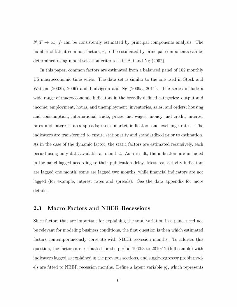
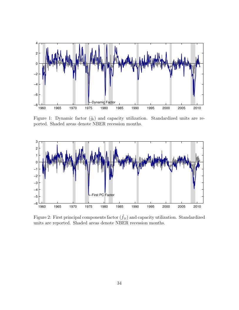
Figure 1 presents the estimated dynamic factor (gt), along with the (standardized)

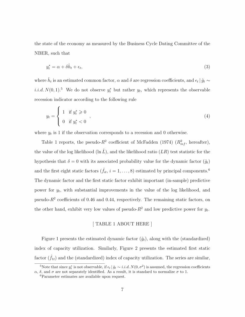
index of capacity utilization. Similarly, Figure 2 presents the estimated first static

factor (f1t) and the (standardized) index of capacity utilization. The series are similar,

5Note that since y∗t is not observable, if εt | gt ∼ i.i.d.N(0, σ2) is assumed, the regression coefficientsα, δ, and σ are not separately identified. As a result, it is standard to normalize σ to 1.

6Parameter estimates are available upon request.

7

with major troughs corresponding closely to NBER recession months (shaded areas).7

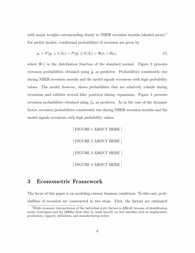
For probit models, conditional probabilities of recession are given by

pt = P (yt = 1 | ht) = P (y∗t > 0 | ht) = Φ(α + δht), (5)

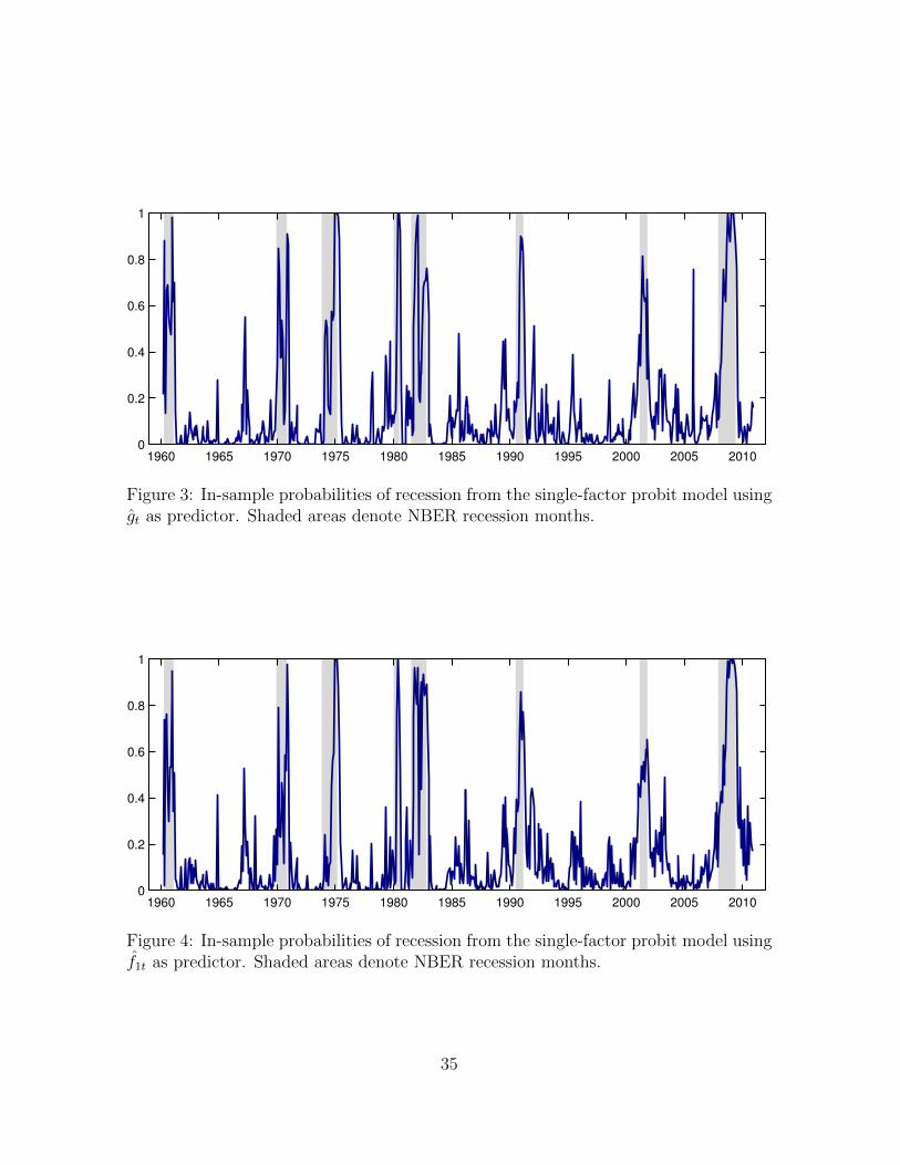
where Φ(·) is the distribution function of the standard normal. Figure 3 presents

recession probabilities obtained using gt as predictor. Probabilities consistently rise

during NBER recession months and the model signals recessions with high probability

values. The model, however, shows probabilities that are relatively volatile during

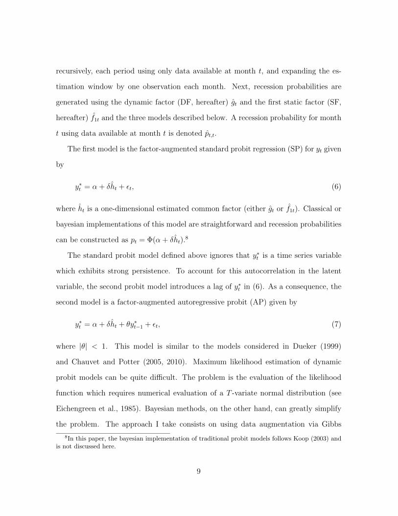
recessions and exhibits several false positives during expansions. Figure 4 presents

recession probabilities obtained using f1t as predictor. As in the case of the dynamic

factor, recession probabilities consistently rise during NBER recession months and the

model signals recessions with high probability values.

[ FIGURE 1 ABOUT HERE ]




3 Econometric Framework

The focus of this paper is on modeling current business conditions. To this end, prob-

abilities of recession are constructed in two steps. First, the factors are estimated

7While economic interpretation of the individual static factors is difficult because of identificationissues, Ludvigson and Ng (2009a) show that f1t loads heavily on real variables such as employment,production, capacity utilization, and manufacturing orders.

8

recursively, each period using only data available at month t, and expanding the es-

timation window by one observation each month. Next, recession probabilities are

generated using the dynamic factor (DF, hereafter) gt and the first static factor (SF,

hereafter) f1t and the three models described below. A recession probability for month

t using data available at month t is denoted pt,t.

The first model is the factor-augmented standard probit regression (SP) for yt given

by

y∗t = α + δht + εt, (6)

where ht is a one-dimensional estimated common factor (either gt or f1t). Classical or

bayesian implementations of this model are straightforward and recession probabilities

can be constructed as pt = Φ(α + δht).8

The standard probit model defined above ignores that y∗t is a time series variable

which exhibits strong persistence. To account for this autocorrelation in the latent

variable, the second probit model introduces a lag of y∗t in (6). As a consequence, the

second model is a factor-augmented autoregressive probit (AP) given by

y∗t = α + δht + θy∗t−1 + εt, (7)

where |θ| < 1. This model is similar to the models considered in Dueker (1999)

and Chauvet and Potter (2005, 2010). Maximum likelihood estimation of dynamic

probit models can be quite difficult. The problem is the evaluation of the likelihood

function which requires numerical evaluation of a T -variate normal distribution (see

Eichengreen et al., 1985). Bayesian methods, on the other hand, can greatly simplify

the problem. The approach I take consists on using data augmentation via Gibbs

8In this paper, the bayesian implementation of traditional probit models follows Koop (2003) andis not discussed here.

9

sampling, allowing to treat y∗t as observed data. The implementation of the Gibbs

sampler for the autoregressive probit model is similar to that of Dueker (1999) and

Chauvet and Potter (2005, 2010) and is discussed in appendix A. As in the case of the

standard probit, recession probabilities can be constructed as pt = Φ(α+ δht + θy∗t−1).

Finally, instead of using binary class models to generate recession probabilities,

we can use Markov-switching models (MS) to generate probabilities directly from the

macro factors as in Diebold and Rudebusch (1996) and Camacho et al. (2013). There-

fore, for the third model it is assumed that the factor ht switches between expansion

and contraction regimes following a mean plus noise specification given by

ht = µst + εt, (8)

where st is defined such that st = 0 during expansions and st = 1 during recessions,

and εt ∼ i.i.d.N(0, σ2ε ). In addition, st is an unobserved two-state first-order Markov

process with transition probabilities given by

p(st = j | st−1 = i) = pij, (9)

where i, j = 0, 1. The regime-switching mean plus noise model can be estimated by

maximum likelihood following Kim and Nelson (1999).9

Predicted probabilities of recession are evaluated using two statistics. The first

statistic is the quadratic probability score (QPS, hereafter), equivalent to the mean

squared error, which is defined by

QPS =1

R

R∑t=1

(yt − pt,t)2, (10)

where R is the number of forecasts and pt,t is the predicted probability of recession

for a given model. The QPS can take values from 0 to 1 and smaller values indicate

9Autoregressive Markov-switching models of order one (as in Diebold and Rudebusch, 1996) andup to four lags were also considered but did not yield better results than the mean plus noise model.This is consistent with the results reported in Camacho et al. (2013).

10

more accurate predictions. Recession probabilities are also evaluated using the log

probability score (LPS, hereafter), which is given by

LPS = − 1

R

R∑t=1

[yt log(pt,t) + (1− yt) log(1− pt,t)] . (11)

The LPS can take values from 0 to +∞ and smaller values indicate more accurate

predictions. Compared to the QPS, the LPS score penalizes large errors more heavily.

See, e.g., Katayama (2010).

4 Results

In total, recession probabilities are constructed using six models. Three of these models

use the small data macro factor gt: (1) a standard probit model with gt as predictor

(DF-SP, hereafter); (2) an autoregressive probit model with gt as predictor (DF-AP,

hereafter); (3) a Markov-switching mean plus noise model for gt (DF-MS, hereafter).

The other three models use the big data macro factor f1t: (4) a standard probit model

with f1t as predictor (SF-SP, hereafter); (5) an autoregressive probit model with f1t

as predictor (SF-AP, hereafter); (6) a Markov-switching mean plus noise model for

f1t (SF-MS, hereafter). Section 4.1 presents out-of-sample results from the forecasting

exercise using ex-post revised data. Sections 4.2 and 4.3 consider the classification of

recession probabilities into binary class predictions using the sequence of probability

forecasts. Finally, section 4.4 presents some results using real-time vintage data (i.e.,

data as it was available at the time the prediction would have been made) instead of

ex-post revised data.

11

4.1 Forecast Evaluation

The out-of-sample forecasting exercise is implemented as follows. First, the two factors

are estimated recursively, each period using only data available at month t (i.e., with

the indicators lagged to account for publication delay), and expanding the estimation

window by one observation each month. Next, the probit and the Markov-switching

models are estimated using the factors obtained in the first step and the end-of-sample

recession probabilities pt,t are constructed for each model. At month t+ 1, the probit

and the Markov-switching models are re-estimated using the factors obtained in the

first step, now using data available at month t + 1, and the end-of-sample recession

probabilities for month t+1 are constructed. This pseudo real-time forecasting exercise

uses ex-post revised data, corresponding to the February 2011 vintage. The initial

estimation sample is from 1960:3 to 1979:1, and the first forecast (nowcast) is for

1979:1. The last forecast corresponds to 2010:12.

The models are estimated as follows. For the probit models, the Gibbs sampler was

run 6,000 iterations and, after discarding the first 1,000 draws to allow the sampler

to converge, results are computed using a thinning factor of 10. Since recent NBER

months are not known, I assume that the forecaster does not know whether the true

state of the economy has changed over the last twelve months. This implies that, at

month t, each probit model is estimated assuming that yt−i = yt−12 for i = 0, 1, ..., 11.10

Since end-of-sample recession probabilities for month t at month t (pt,t) are generated

without making use of yt or month t data, these are in fact out-of-sample recession

10The implementation of the Gibbs sampler for probit models involves sampling values of the latentvariable y∗t from a truncated normal distribution where y∗t ≥ 0 if yt = 1 and y∗t < 0 if yt = 0. Sincerecent values of yt are not known, the probit models are estimated with the last twelve observationssampled without imposing this truncation. The effect of this is that the latent variable y∗t is allowedto move freely without being conditioned by yt and, as a result, for estimation (and forecasting) thevalues of yt−i for i = 0, . . . , 11 are not relevant. See appendix A for more details.

12

probabilities. In the case of the Markov-switching models, at each month t the model

is estimated by maximum likelihood as explained in the previous section.

Table 2 reports the out-of-sample QPS and LPS for the six models over the period

1979.1 – 2010:12. In addition to reporting the results for all months, Table 2 also

reports separate results for NBER defined expansion and recession months. These two

statistics describe a consistent picture: model SF-SP generates the series of end-of-

sample recession probabilities that better fits subsequently declared NBER recession

months. In addition, this model also exhibits the best performance when looking at

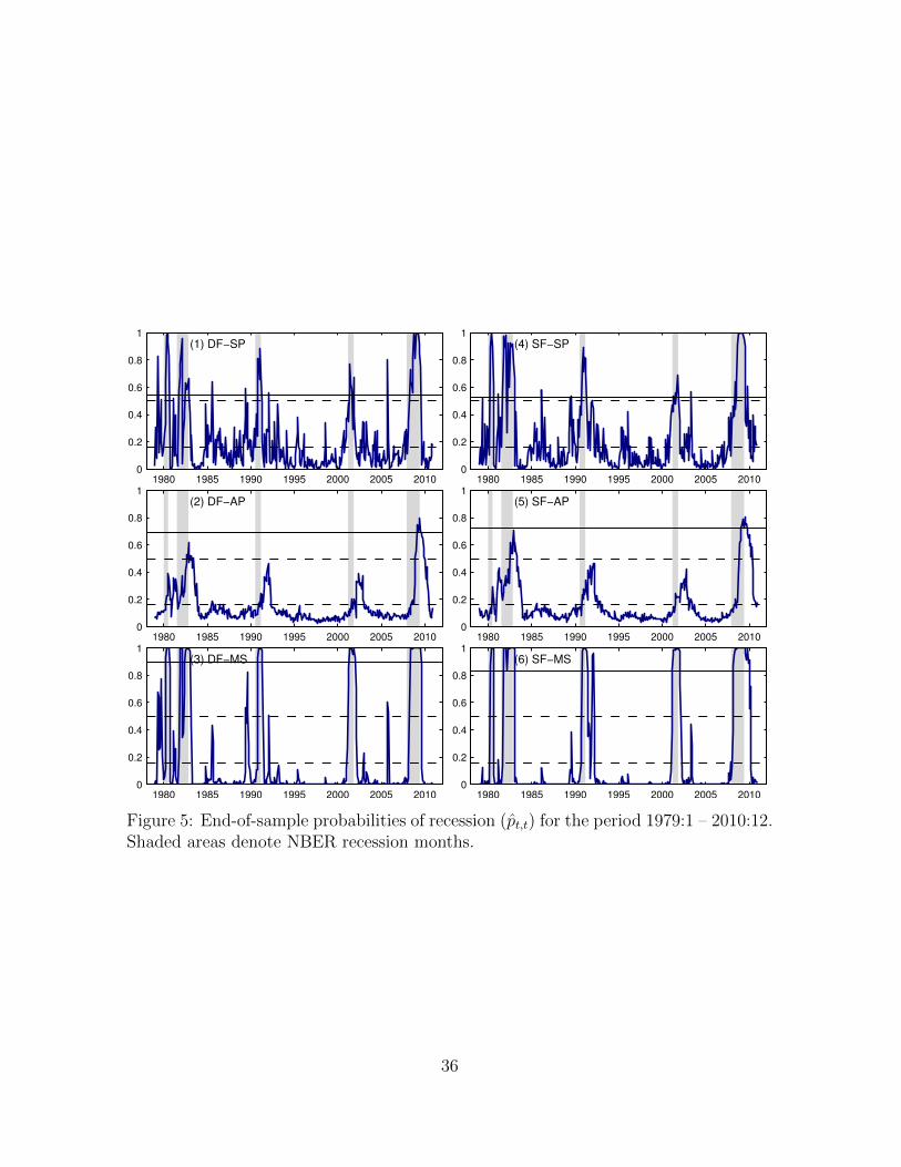
recession months only. Figure 5 presents the end-of-sample probabilities of recession

pt,t for the six models considered. We observe that the standard probit models gener-

ate recession probabilities that consistently rise during subsequently declared NBER

recession months. Model DF-SP, however, shows relatively lower and more volatile

probabilities during recessions (and a higher QPS value) than model SF-SP. The au-

toregressive probit models, on the other hand, exhibit a poor performance, generating

probabilities that are smooth but very low during NBER recession months and yielding

significantly delayed recession calls. As a result, the autoregressive probit models fail

to identify the 1990/91 and 2001 recessions with high probabilities and only identify

other recessions with an important lag. The Markov-switching models, on the other

hand, generate recession probabilities that are smooth, high during NBER recession

months, and generally close to zero during expansions.



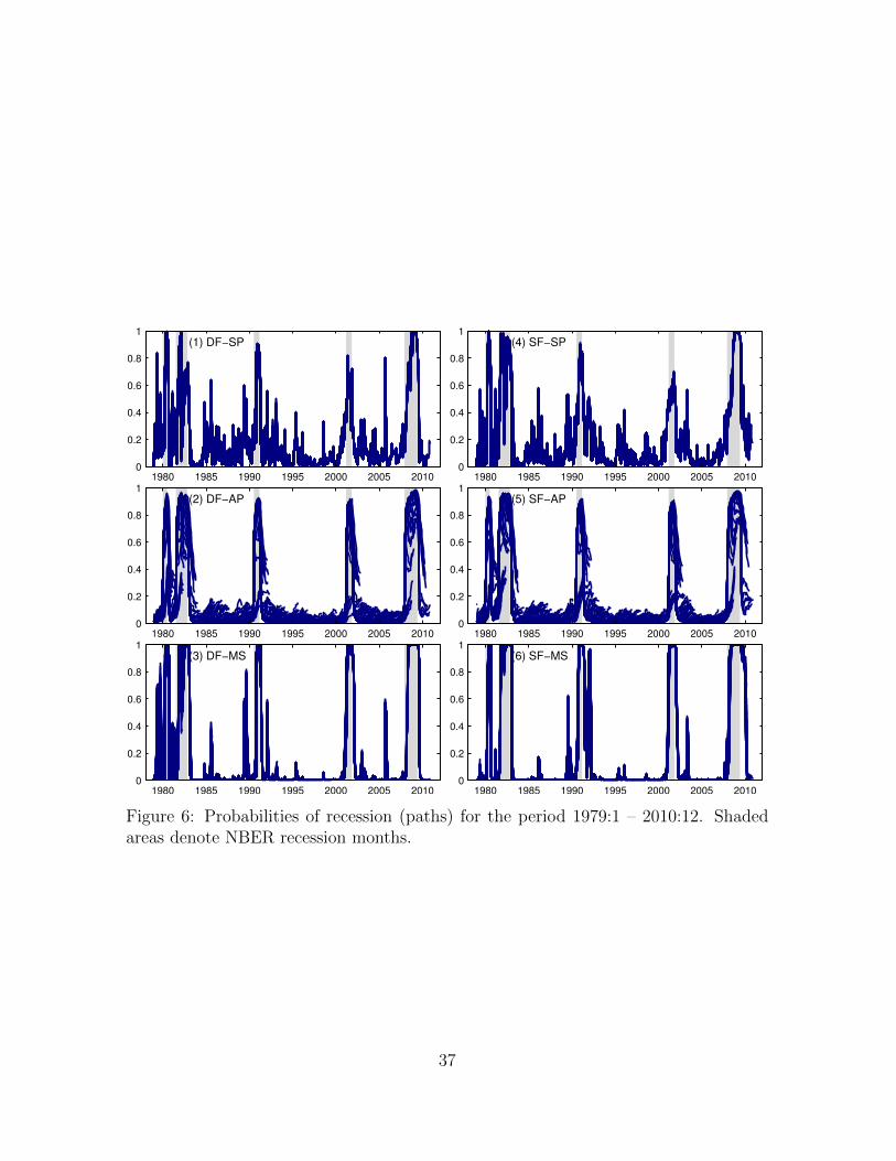
Figure 6 presents the full paths of recession probabilities from which the end-of-

sample probabilities are obtained (tentacle plot). In the case of the standard probit

13

and the Markov-switching models, the probability paths do not exhibit much varia-

tion as more data is incorporated and, as a result, in- and end-of-sample estimated

probabilities are similar. The results for the autoregressive probit models, on the other

hand, are quite different. In this case, the paths exhibit important changes as ad-

ditional observations are added to the sample and this issue is particularly evident

during NBER recession months. The probability paths computed from the autoregres-

sive probit models are very persistent, explaining the delayed recession calls noticed

above (Figure 5).11


4.2 Binary Class Predictions

A formal evaluation of the end-of-sample probabilities as predictors of NBER recession

months requires the selection of a classification rule and a loss function for binary class

predictions that reflects the preferences of the forecaster. In the case of recession indi-

cators, the loss can be considered greater in the case of missed signals and, as a result,

an asymmetric loss function may be appropriate. The cost-weighted misclassification

loss function (ML, hereafter) assumes that the two types of misclassifications (false

positives and false negatives) involve differing costs while assuming that the sum of

costs add to 1 (see, e.g., Buja et al., 2005). The ML function is given by

ML =1

R

R∑t=1

((1− q)yt(1− yt,t) + q(1− yt)yt,t

), (12)

11In contrast, both autoregressive probit models exhibit an almost perfect in-sample fit (resultsnot reported). Similar in-sample results are reported in Chauvet and Potter (2010). For in-sampleestimation, the autoregressive probit models use the values of yt to accurately fit NBER recessionmonths. But this information is exactly what is not available in real-time and in the pseudo real-timeforecasting exercise. As a result, the out-of-sample performance of these models exhibits a substantialdeterioration.

14

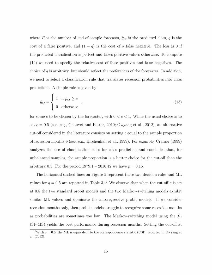
where R is the number of end-of-sample forecasts, yt,t is the predicted class, q is the

cost of a false positive, and (1 − q) is the cost of a false negative. The loss is 0 if

the predicted classification is perfect and takes positive values otherwise. To compute

(12) we need to specify the relative cost of false positives and false negatives. The

choice of q is arbitrary, but should reflect the preferences of the forecaster. In addition,

we need to select a classification rule that translates recession probabilities into class

predictions. A simple rule is given by

yt,t =

1 if pt,t ≥ c

0 otherwise, (13)

for some c to be chosen by the forecaster, with 0 < c < 1. While the usual choice is to

set c = 0.5 (see, e.g., Chauvet and Potter, 2010; Owyang et al., 2012), an alternative

cut-off considered in the literature consists on setting c equal to the sample proportion

of recession months p (see, e.g., Birchenhall et al., 1999). For example, Cramer (1999)

analyzes the use of classification rules for class prediction and concludes that, for

unbalanced samples, the sample proportion is a better choice for the cut-off than the

arbitrary 0.5. For the period 1979.1 – 2010:12 we have p = 0.16.

The horizontal dashed lines on Figure 5 represent these two decision rules and ML

values for q = 0.5 are reported in Table 3.12 We observe that when the cut-off c is set

at 0.5 the two standard probit models and the two Markov-switching models exhibit

similar ML values and dominate the autoregressive probit models. If we consider

recession months only, then probit models struggle to recognize some recession months

as probabilities are sometimes too low. The Markov-switching model using the f1t

(SF-MS) yields the best performance during recession months. Setting the cut-off at

12With q = 0.5, the ML is equivalent to the correspondence statistic (CSP) reported in Owyang etal. (2012).

15

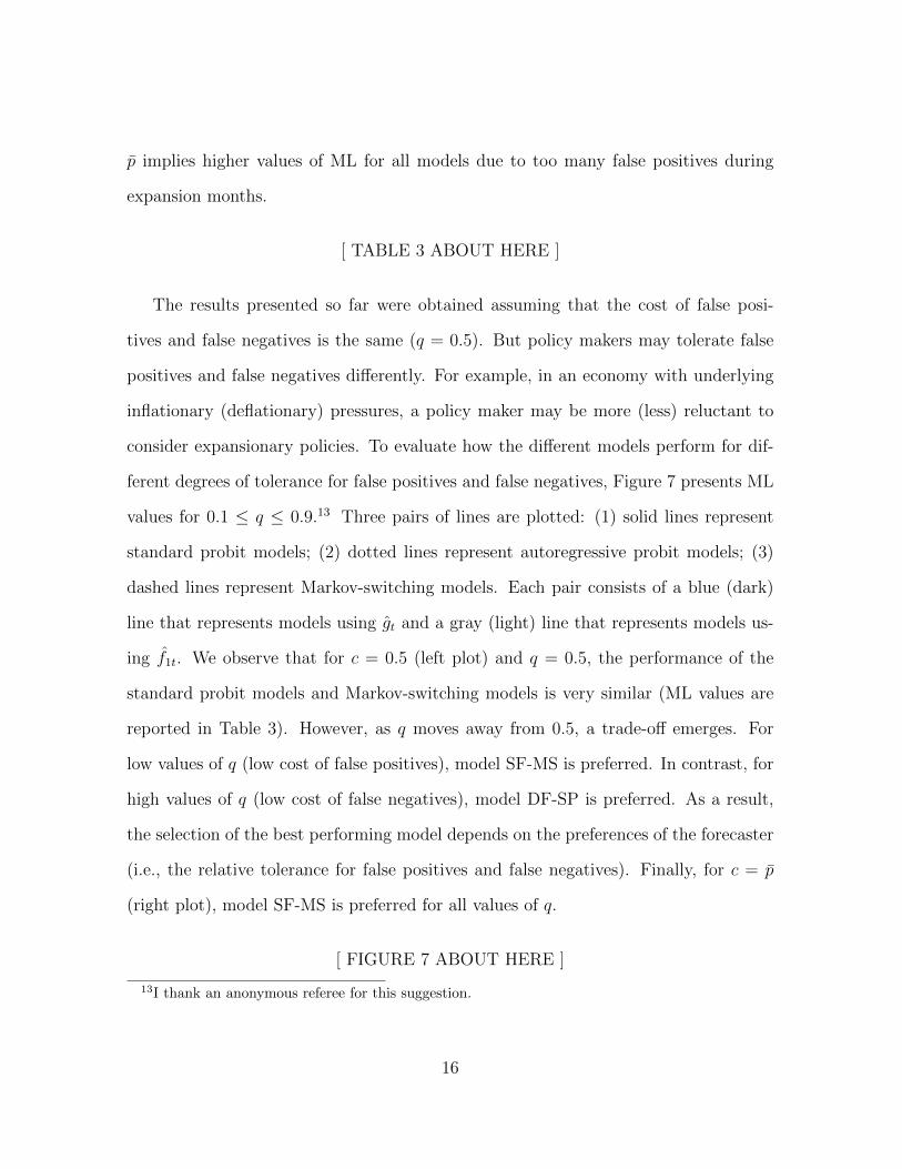
p implies higher values of ML for all models due to too many false positives during

expansion months.


The results presented so far were obtained assuming that the cost of false posi-

tives and false negatives is the same (q = 0.5). But policy makers may tolerate false

positives and false negatives differently. For example, in an economy with underlying

inflationary (deflationary) pressures, a policy maker may be more (less) reluctant to

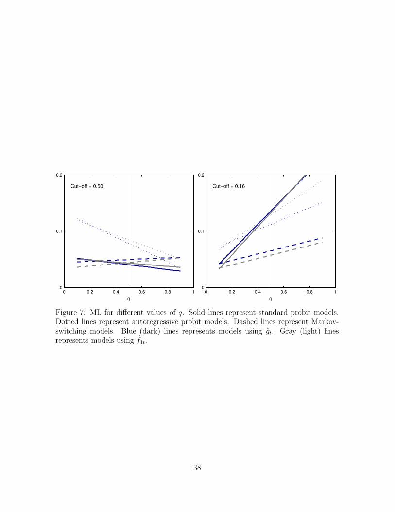
consider expansionary policies. To evaluate how the different models perform for dif-

ferent degrees of tolerance for false positives and false negatives, Figure 7 presents ML

values for 0.1 ≤ q ≤ 0.9.13 Three pairs of lines are plotted: (1) solid lines represent

standard probit models; (2) dotted lines represent autoregressive probit models; (3)

dashed lines represent Markov-switching models. Each pair consists of a blue (dark)

line that represents models using gt and a gray (light) line that represents models us-

ing f1t. We observe that for c = 0.5 (left plot) and q = 0.5, the performance of the

standard probit models and Markov-switching models is very similar (ML values are

reported in Table 3). However, as q moves away from 0.5, a trade-off emerges. For

low values of q (low cost of false positives), model SF-MS is preferred. In contrast, for

high values of q (low cost of false negatives), model DF-SP is preferred. As a result,

the selection of the best performing model depends on the preferences of the forecaster

(i.e., the relative tolerance for false positives and false negatives). Finally, for c = p

(right plot), model SF-MS is preferred for all values of q.


13I thank an anonymous referee for this suggestion.

16

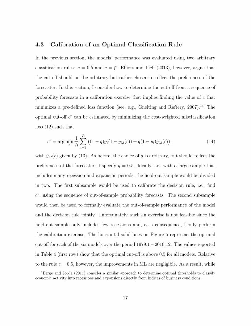
4.3 Calibration of an Optimal Classification Rule

In the previous section, the models’ performance was evaluated using two arbitrary

classification rules: c = 0.5 and c = p. Elliott and Lieli (2013), however, argue that

the cut-off should not be arbitrary but rather chosen to reflect the preferences of the

forecaster. In this section, I consider how to determine the cut-off from a sequence of

probability forecasts in a calibration exercise that implies finding the value of c that

minimizes a pre-defined loss function (see, e.g., Gneiting and Raftery, 2007).14 The

optimal cut-off c∗ can be estimated by minimizing the cost-weighted misclassification

loss (12) such that

c∗ = arg minc

1

R

R∑t=1

((1− q)yt(1− yt,t(c)) + q(1− yt)yt,t(c)

), (14)

with yt,t(c) given by (13). As before, the choice of q is arbitrary, but should reflect the

preferences of the forecaster. I specify q = 0.5. Ideally, i.e. with a large sample that

includes many recession and expansion periods, the hold-out sample would be divided

in two. The first subsample would be used to calibrate the decision rule, i.e. find

c∗, using the sequence of out-of-sample probability forecasts. The second subsample

would then be used to formally evaluate the out-of-sample performance of the model

and the decision rule jointly. Unfortunately, such an exercise is not feasible since the

hold-out sample only includes few recessions and, as a consequence, I only perform

the calibration exercise. The horizontal solid lines on Figure 5 represent the optimal

cut-off for each of the six models over the period 1979:1 – 2010:12. The values reported

in Table 4 (first row) show that the optimal cut-off is above 0.5 for all models. Relative

to the rule c = 0.5, however, the improvements in ML are negligible. As a result, while

14Berge and Jorda (2011) consider a similar approach to determine optimal thresholds to classifyeconomic activity into recessions and expansions directly from indices of business conditions.

17

the rule c = 0.5 is arbitrary, it appears to works as well as a rule based on the optimal

cut-off c∗. As before, model SF-MS exhibits the best performance.


4.4 Forecast Evaluation with Real-Time Data

All the results presented above were obtained using ex-post revised data corresponding

to the February 2011 vintage. In this section, I evaluate the robustness of the out-

of-sample forecasting results using data as it was available at the time the prediction

would have been made (vintage data) instead of ex-post revised data. As before, the

dynamic factor is estimated recursively, now using data as it was available at month

t. In this case, however, the four indicators are lagged two months to account for

publication delay and important revisions that are usually observed in the first and

the second release (see Chauvet and Piger, 2008). Unfortunately, a real-time vintage

data set of the 102 indicators included in the large panel is not available. Instead,

I use real-time monthly estimates of Chicago Fed National Activity Index (CFNAI)

constructed by the Federal Reserve Bank of Chicago which are available as it was

originally published at the time of release. The CFNAI is a monthly index, designed

to measure overall economic activity, estimated as the first principal component from

a panel of 85 indicators of national economic activity.15 The real-time data sets cover

the period 1967:3 to 2010:12. The first available vintage corresponds to 2001:1 and the

last to 2010:12, which includes the two most recent NBER recessions.

Table 5 reports the out-of-sample QPS and LPS for the six models over the period

2001.1 – 2010:12 using real-time data. The two statistics describe a consistent picture

15Note that while there is some overlap, the CFNAI is estimated using a panel of 85 economicactivity indicators while f1t is estimated using a broader panel of 102 indicators.https://www.chicagofed.org/publications/cfnai/index

18

with the results obtained using ex-post revised data. Standard probit models and

Markov-switching models generate the series of end-of-sample recession probabilities

that better fit subsequently declared NBER recession months. In addition, probit

models show more volatile probabilities while the Markov-switching models generate

recession probabilities that are smooth, high during NBER recession months, and

generally close to zero during expansions. Finally, we observe that models using the

CFNAI exhibit a better performance than those using the dynamic factor.


5 Conclusion

This paper provides an assessment of the predictive power of macro factors for current

US recessions using both binary class models and Markov-switching models. Instead of

relying on a small number of observed variables, these models are built around latent

common factors estimated from small and large data sets of macroeconomic indicators.

Both macro factors have important predictive power for NBER recession months and

can be used to assess current business conditions. Markov-switching models are found

to be more conservative, showing fewer false positives at the cost of some missed

signals (mainly delayed calls). On the other hand, standard probit models detect most

peaks and troughs sooner but exhibit more volatile probabilities. Overall, a simple

Markov-switching model based on the big data macro factor generates the sequence

of out-of-sample class predictions that better approximates NBER recession months.

Nevertheless, it is shown that the selection of the best performing model depends on

the forecaster’s relative tolerance for false positives and false negatives and, as a result,

some forecasters may prefer other models.

19

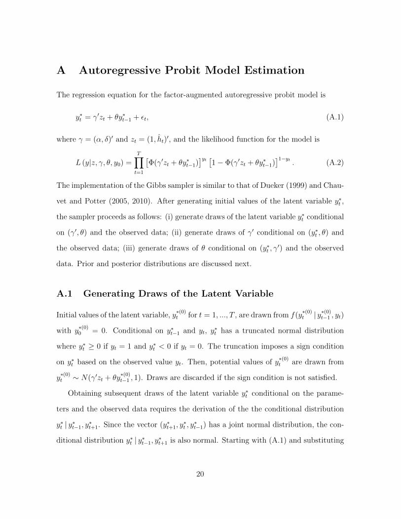
A Autoregressive Probit Model Estimation

The regression equation for the factor-augmented autoregressive probit model is

y∗t = γ′zt + θy∗t−1 + εt, (A.1)

where γ = (α, δ)′ and zt = (1, ht)′, and the likelihood function for the model is

L (y|z, γ, θ, y0) =T∏t=1

[Φ(γ′zt + θy∗t−1)

]yt [1− Φ(γ′zt + θy∗t−1)

]1−yt. (A.2)

The implementation of the Gibbs sampler is similar to that of Dueker (1999) and Chau-

vet and Potter (2005, 2010). After generating initial values of the latent variable y∗t ,

the sampler proceeds as follows: (i) generate draws of the latent variable y∗t conditional

on (γ′, θ) and the observed data; (ii) generate draws of γ′ conditional on (y∗t , θ) and

the observed data; (iii) generate draws of θ conditional on (y∗t , γ′) and the observed

data. Prior and posterior distributions are discussed next.

A.1 Generating Draws of the Latent Variable

Initial values of the latent variable, y∗(0)t for t = 1, ..., T , are drawn from f(y

∗(0)t | y∗(0)

t−1 , yt)

with y∗(0)0 = 0. Conditional on y∗t−1 and yt, y

∗t has a truncated normal distribution

where y∗t ≥ 0 if yt = 1 and y∗t < 0 if yt = 0. The truncation imposes a sign condition

on y∗t based on the observed value yt. Then, potential values of y∗(0)t are drawn from

y∗(0)t ∼ N(γ′zt + θy

∗(0)t−1 , 1). Draws are discarded if the sign condition is not satisfied.

Obtaining subsequent draws of the latent variable y∗t conditional on the parame-

ters and the observed data requires the derivation of the the conditional distribution

y∗t | y∗t−1, y∗t+1. Since the vector (y∗t+1, y

∗t , y∗t−1) has a joint normal distribution, the con-

ditional distribution y∗t | y∗t−1, y∗t+1 is also normal. Starting with (A.1) and substituting

20

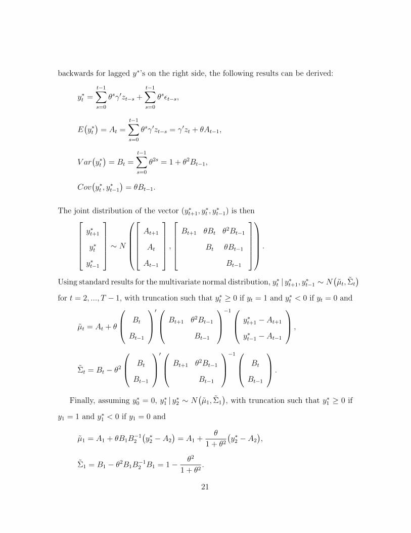
backwards for lagged y∗’s on the right side, the following results can be derived:

y∗t =t−1∑s=0

θsγ′zt−s +t−1∑s=0

θsεt−s,

E(y∗t)

= At =t−1∑s=0

θsγ′zt−s = γ′zt + θAt−1,

V ar(y∗t)

= Bt =t−1∑s=0

θ2s = 1 + θ2Bt−1,

Cov(y∗t , y

∗t−1

)= θBt−1.

The joint distribution of the vector (y∗t+1, y∗t , y∗t−1) is then

y∗t+1

y∗t

y∗t−1

∼ N

At+1

At

At−1

,Bt+1 θBt θ2Bt−1

Bt θBt−1

Bt−1

.

Using standard results for the multivariate normal distribution, y∗t | y∗t+1, y∗t−1 ∼ N

(µt, Σt

)for t = 2, ..., T − 1, with truncation such that y∗t ≥ 0 if yt = 1 and y∗t < 0 if yt = 0 and

µt = At + θ

Bt

Bt−1

′ Bt+1 θ2Bt−1

Bt−1

−1 y∗t+1 − At+1

y∗t−1 − At−1

,

Σt = Bt − θ2

Bt

Bt−1

′ Bt+1 θ2Bt−1

Bt−1

−1 Bt

Bt−1

.

Finally, assuming y∗0 = 0, y∗1 | y∗2 ∼ N(µ1, Σ1

), with truncation such that y∗1 ≥ 0 if

y1 = 1 and y∗1 < 0 if y1 = 0 and

µ1 = A1 + θB1B−12

(y∗2 − A2

)= A1 +

θ

1 + θ2

(y∗2 − A2

),

Σ1 = B1 − θ2B1B−12 B1 = 1− θ2

1 + θ2.

21

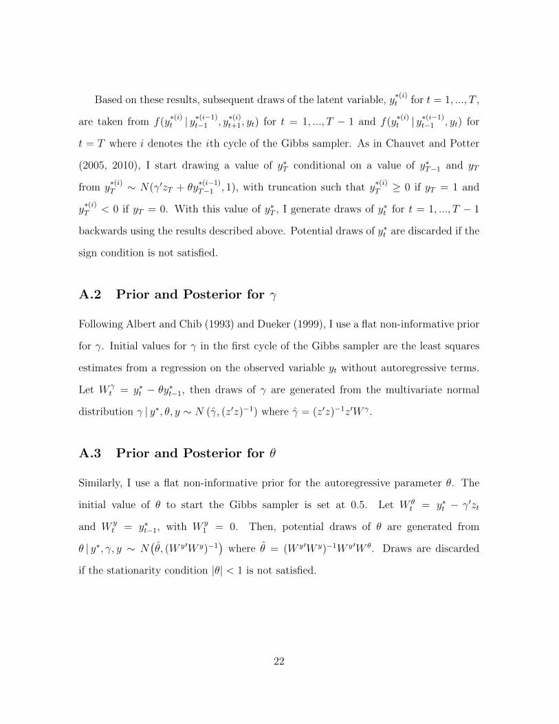
Based on these results, subsequent draws of the latent variable, y∗(i)t for t = 1, ..., T ,

are taken from f(y∗(i)t | y∗(i−1)

t−1 , y∗(i)t+1, yt) for t = 1, ..., T − 1 and f(y

∗(i)t | y∗(i−1)

t−1 , yt) for

t = T where i denotes the ith cycle of the Gibbs sampler. As in Chauvet and Potter

(2005, 2010), I start drawing a value of y∗T conditional on a value of y∗T−1 and yT

from y∗(i)T ∼ N(γ′zT + θy

∗(i−1)T−1 , 1), with truncation such that y

∗(i)T ≥ 0 if yT = 1 and

y∗(i)T < 0 if yT = 0. With this value of y∗T , I generate draws of y∗t for t = 1, ..., T − 1

backwards using the results described above. Potential draws of y∗t are discarded if the

sign condition is not satisfied.

A.2 Prior and Posterior for γ

Following Albert and Chib (1993) and Dueker (1999), I use a flat non-informative prior

for γ. Initial values for γ in the first cycle of the Gibbs sampler are the least squares

estimates from a regression on the observed variable yt without autoregressive terms.

Let W γt = y∗t − θy∗t−1, then draws of γ are generated from the multivariate normal

distribution γ | y∗, θ, y ∼ N (γ, (z′z)−1) where γ = (z′z)−1z′W γ.

A.3 Prior and Posterior for θ

Similarly, I use a flat non-informative prior for the autoregressive parameter θ. The

initial value of θ to start the Gibbs sampler is set at 0.5. Let W θt = y∗t − γ′zt

and W yt = y∗t−1, with W y

1 = 0. Then, potential draws of θ are generated from

θ | y∗, γ, y ∼ N(θ, (W y ′W y)−1

)where θ = (W y ′W y)−1W y ′W θ. Draws are discarded

if the stationarity condition |θ| < 1 is not satisfied.

22

A.4 Recession Probabilities

Conditional recession probabilities are generated at each draw of the Gibbs sampler

such that

p(i)t = Φ

(γ(i)′zt + θ(i)y

∗(i)t−1

), (A.3)

where i denotes the ith cycle of the Gibbs sampler. The posterior mean probability of

recession is given by

pt =1

I

I∑i=1

p(i)t , (A.4)

where I denotes the total number of draws.

B Data Appendix

A data set of the four indicators used to estimate the dynamic factor (industrial pro-

duction, real manufacturing sales, real personal income less transfer payments, and

employment) corresponding to the February 2011 vintage was provided by Jeremy

Piger. Real-time vintage data for the dynamic factor is from Camacho et al. (2013).

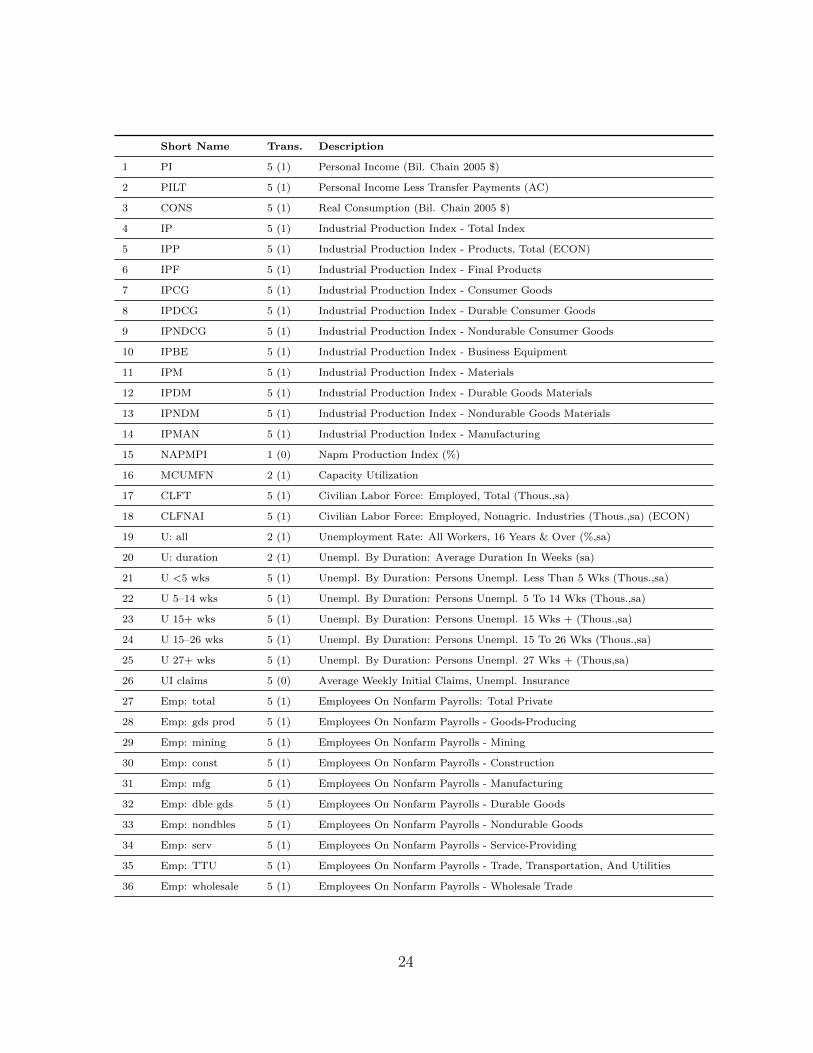
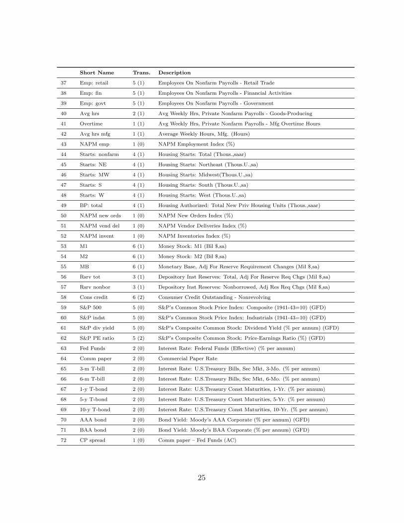
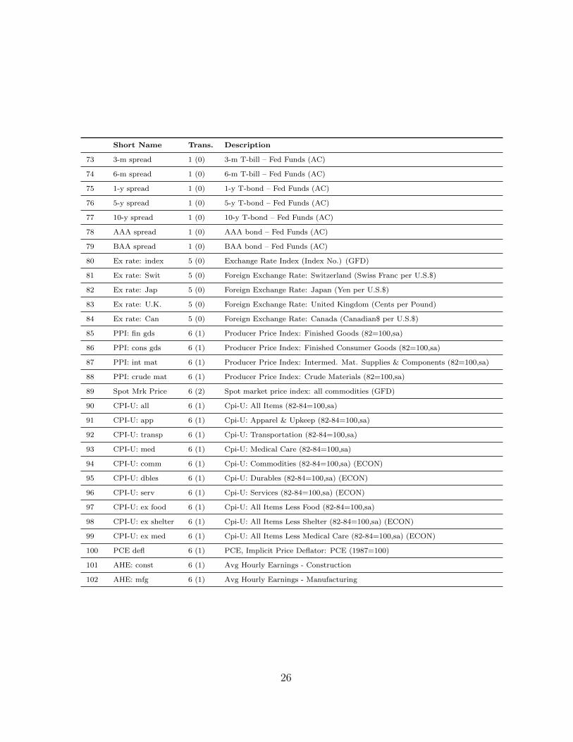
The table below lists the 102 time series included in the balanced panel. The table

lists the short name of each series, the transformation applied (number of months to

be lagged in parentheses), and a brief data description. All series are from FRED –

St. Louis Fed –, unless the source is listed as ECON (Economagic), GFD (Global

Financial Data), or AC (author’s calculation) and correspond to the February 2011

vintage. The transformation codes are: 1 = no transformation; 2 = first difference;

3 = second difference; 4 = logarithm; 5 = first difference of logarithms; 6 = second

difference of logarithms.

23

Short Name Trans. Description

1 PI 5 (1) Personal Income (Bil. Chain 2005 $)

2 PILT 5 (1) Personal Income Less Transfer Payments (AC)

3 CONS 5 (1) Real Consumption (Bil. Chain 2005 $)

4 IP 5 (1) Industrial Production Index - Total Index

5 IPP 5 (1) Industrial Production Index - Products, Total (ECON)

6 IPF 5 (1) Industrial Production Index - Final Products

7 IPCG 5 (1) Industrial Production Index - Consumer Goods

8 IPDCG 5 (1) Industrial Production Index - Durable Consumer Goods

9 IPNDCG 5 (1) Industrial Production Index - Nondurable Consumer Goods

10 IPBE 5 (1) Industrial Production Index - Business Equipment

11 IPM 5 (1) Industrial Production Index - Materials

12 IPDM 5 (1) Industrial Production Index - Durable Goods Materials

13 IPNDM 5 (1) Industrial Production Index - Nondurable Goods Materials

14 IPMAN 5 (1) Industrial Production Index - Manufacturing

15 NAPMPI 1 (0) Napm Production Index (%)

16 MCUMFN 2 (1) Capacity Utilization

17 CLFT 5 (1) Civilian Labor Force: Employed, Total (Thous.,sa)

18 CLFNAI 5 (1) Civilian Labor Force: Employed, Nonagric. Industries (Thous.,sa) (ECON)

19 U: all 2 (1) Unemployment Rate: All Workers, 16 Years & Over (%,sa)

20 U: duration 2 (1) Unempl. By Duration: Average Duration In Weeks (sa)

21 U <5 wks 5 (1) Unempl. By Duration: Persons Unempl. Less Than 5 Wks (Thous.,sa)

22 U 5–14 wks 5 (1) Unempl. By Duration: Persons Unempl. 5 To 14 Wks (Thous.,sa)

23 U 15+ wks 5 (1) Unempl. By Duration: Persons Unempl. 15 Wks + (Thous.,sa)

24 U 15–26 wks 5 (1) Unempl. By Duration: Persons Unempl. 15 To 26 Wks (Thous.,sa)

25 U 27+ wks 5 (1) Unempl. By Duration: Persons Unempl. 27 Wks + (Thous,sa)

26 UI claims 5 (0) Average Weekly Initial Claims, Unempl. Insurance

27 Emp: total 5 (1) Employees On Nonfarm Payrolls: Total Private

28 Emp: gds prod 5 (1) Employees On Nonfarm Payrolls - Goods-Producing

29 Emp: mining 5 (1) Employees On Nonfarm Payrolls - Mining

30 Emp: const 5 (1) Employees On Nonfarm Payrolls - Construction

31 Emp: mfg 5 (1) Employees On Nonfarm Payrolls - Manufacturing

32 Emp: dble gds 5 (1) Employees On Nonfarm Payrolls - Durable Goods

33 Emp: nondbles 5 (1) Employees On Nonfarm Payrolls - Nondurable Goods

34 Emp: serv 5 (1) Employees On Nonfarm Payrolls - Service-Providing

35 Emp: TTU 5 (1) Employees On Nonfarm Payrolls - Trade, Transportation, And Utilities

36 Emp: wholesale 5 (1) Employees On Nonfarm Payrolls - Wholesale Trade

24


37 Emp: retail 5 (1) Employees On Nonfarm Payrolls - Retail Trade

38 Emp: fin 5 (1) Employees On Nonfarm Payrolls - Financial Activities

39 Emp: govt 5 (1) Employees On Nonfarm Payrolls - Government

40 Avg hrs 2 (1) Avg Weekly Hrs, Private Nonfarm Payrolls - Goods-Producing

41 Overtime 1 (1) Avg Weekly Hrs, Private Nonfarm Payrolls - Mfg Overtime Hours

42 Avg hrs mfg 1 (1) Average Weekly Hours, Mfg. (Hours)

43 NAPM emp 1 (0) NAPM Employment Index (%)

44 Starts: nonfarm 4 (1) Housing Starts: Total (Thous.,saar)

45 Starts: NE 4 (1) Housing Starts: Northeast (Thous.U.,sa)

46 Starts: MW 4 (1) Housing Starts: Midwest(Thous.U.,sa)

47 Starts: S 4 (1) Housing Starts: South (Thous.U.,sa)

48 Starts: W 4 (1) Housing Starts: West (Thous.U.,sa)

49 BP: total 4 (1) Housing Authorized: Total New Priv Housing Units (Thous.,saar)

50 NAPM new ords 1 (0) NAPM New Orders Index (%)

51 NAPM vend del 1 (0) NAPM Vendor Deliveries Index (%)

52 NAPM invent 1 (0) NAPM Inventories Index (%)

53 M1 6 (1) Money Stock: M1 (Bil $,sa)

54 M2 6 (1) Money Stock: M2 (Bil $,sa)

55 MB 6 (1) Monetary Base, Adj For Reserve Requirement Changes (Mil $,sa)

56 Rsrv tot 3 (1) Depository Inst Reserves: Total, Adj For Reserve Req Chgs (Mil $,sa)

57 Rsrv nonbor 3 (1) Depository Inst Reserves: Nonborrowed, Adj Res Req Chgs (Mil $,sa)

58 Cons credit 6 (2) Consumer Credit Outstanding - Nonrevolving

59 S&P 500 5 (0) S&P’s Common Stock Price Index: Composite (1941-43=10) (GFD)

60 S&P indst 5 (0) S&P’s Common Stock Price Index: Industrials (1941-43=10) (GFD)

61 S&P div yield 5 (0) S&P’s Composite Common Stock: Dividend Yield (% per annum) (GFD)

62 S&P PE ratio 5 (2) S&P’s Composite Common Stock: Price-Earnings Ratio (%) (GFD)

63 Fed Funds 2 (0) Interest Rate: Federal Funds (Effective) (% per annum)

64 Comm paper 2 (0) Commercial Paper Rate

65 3-m T-bill 2 (0) Interest Rate: U.S.Treasury Bills, Sec Mkt, 3-Mo. (% per annum)

66 6-m T-bill 2 (0) Interest Rate: U.S.Treasury Bills, Sec Mkt, 6-Mo. (% per annum)

67 1-y T-bond 2 (0) Interest Rate: U.S.Treasury Const Maturities, 1-Yr. (% per annum)



70 AAA bond 2 (0) Bond Yield: Moody’s AAA Corporate (% per annum) (GFD)

71 BAA bond 2 (0) Bond Yield: Moody’s BAA Corporate (% per annum) (GFD)

72 CP spread 1 (0) Comm paper – Fed Funds (AC)

25


73 3-m spread 1 (0) 3-m T-bill – Fed Funds (AC)

74 6-m spread 1 (0) 6-m T-bill – Fed Funds (AC)

75 1-y spread 1 (0) 1-y T-bond – Fed Funds (AC)



78 AAA spread 1 (0) AAA bond – Fed Funds (AC)

79 BAA spread 1 (0) BAA bond – Fed Funds (AC)

80 Ex rate: index 5 (0) Exchange Rate Index (Index No.) (GFD)

81 Ex rate: Swit 5 (0) Foreign Exchange Rate: Switzerland (Swiss Franc per U.S.$)

82 Ex rate: Jap 5 (0) Foreign Exchange Rate: Japan (Yen per U.S.$)

83 Ex rate: U.K. 5 (0) Foreign Exchange Rate: United Kingdom (Cents per Pound)

84 Ex rate: Can 5 (0) Foreign Exchange Rate: Canada (Canadian$ per U.S.$)

85 PPI: fin gds 6 (1) Producer Price Index: Finished Goods (82=100,sa)

86 PPI: cons gds 6 (1) Producer Price Index: Finished Consumer Goods (82=100,sa)

87 PPI: int mat 6 (1) Producer Price Index: Intermed. Mat. Supplies & Components (82=100,sa)

88 PPI: crude mat 6 (1) Producer Price Index: Crude Materials (82=100,sa)

89 Spot Mrk Price 6 (2) Spot market price index: all commodities (GFD)

90 CPI-U: all 6 (1) Cpi-U: All Items (82-84=100,sa)

91 CPI-U: app 6 (1) Cpi-U: Apparel & Upkeep (82-84=100,sa)

92 CPI-U: transp 6 (1) Cpi-U: Transportation (82-84=100,sa)

93 CPI-U: med 6 (1) Cpi-U: Medical Care (82-84=100,sa)

94 CPI-U: comm 6 (1) Cpi-U: Commodities (82-84=100,sa) (ECON)

95 CPI-U: dbles 6 (1) Cpi-U: Durables (82-84=100,sa) (ECON)

96 CPI-U: serv 6 (1) Cpi-U: Services (82-84=100,sa) (ECON)

97 CPI-U: ex food 6 (1) Cpi-U: All Items Less Food (82-84=100,sa)

98 CPI-U: ex shelter 6 (1) Cpi-U: All Items Less Shelter (82-84=100,sa) (ECON)

99 CPI-U: ex med 6 (1) Cpi-U: All Items Less Medical Care (82-84=100,sa) (ECON)

100 PCE defl 6 (1) PCE, Implicit Price Deflator: PCE (1987=100)

101 AHE: const 6 (1) Avg Hourly Earnings - Construction

102 AHE: mfg 6 (1) Avg Hourly Earnings - Manufacturing

26

References

Albert, J.H., and Chib, S. (1993): “Bayesian Analysis of Binary and Polychotomous

Response Data”, Journal of the American Statistical Association, 88, 669–679.

Aruoba, S.B., Diebold, F.X., and Scotti, C. (2009): “Real-Time Measurement of Busi-

ness Conditions”, Journal of Business and Economic Statistics, 27(4), 417–427.

Bai, J., and Ng, S. (2002): “Determining the Number of Factors in Approximate Factor

Models”, Econometrica, 70, 191–221.

Berge, T.J., and Jorda, O. (2011): “Evaluating the Classification of Economic Activity

in Recessions and Expansions”, American Economic Journal: Macroeconomics, 3,

246–277.

Birchenhall, C.R., Jessen, H., Osborn, D.R., Simpson, P. (1999): “Predicting U.S.

Business-Cycle Regimes”, Journal of Business and Economic Statistics, 17(3), 313–

323.

Buja, A., Stuetzle, W., and Shen, Y. (2005): “Loss Functions for Binary Class Proba-

bility Estimation and Classification: Structure and Applications”, unpublished.

Camacho, M., Perez-Quiros, G., and Poncela, P. (2013): “Extracting Nonlinear Signals

from Several Economic Indicators”, Documento de Trabajo 1202, Banco de Espana.

Chauvet, M. (1998): “An Econometric Characterization of Business Cycle Dynamics

with Factor Structure and Regime Switches”, International Economic Review, 39(4),

969–996.

Chauvet, M., and Hamilton, J. D. (2006): “Dating Business Cycle Turning Points”, in

27

Non-linear Time Series Analysis of Business Cycles, ed. by D. van Dijk, C. Milas,

and P. Rothman, Contributions to Economic Analysis series, 276, 1–54. Elsevier.

Chauvet, M., and Piger, J. (2008): “A Comparison of the Real-Time Performance of

Business Cycle Dating Methods”, Journal of Business and Economic Statistics, 26,

42–49.

Chauvet, M., and Potter, S. (2002): “Predicting Recessions: Evidence from the Yield

Curve in the Presence of Structural Breaks”, Economic Letters, 77(2), 245–253.

Chauvet, M., and Potter, S. (2005): “Forecasting Recessions Using the Yield Curve”,

Journal of Forecasting, 24(2), 77–103.

Chauvet, M., and Potter, S. (2010): “Business Cycle Monitoring with Structural

Changes”, International Journal of Forecasting, 26 (4), 777–793.

Cramer, J.S. (1999): “Predictive Performance of the Binary Logit Model in Unbalanced

Samples”, Journal of the Royal Statistical Society, Series D (The Statistician), 48(1),

85–94.

Diebold, F., and Rudebusch, G. (1996): “Measuring Business Cycles: A Modern Per-

spective”, Review of Economics and Statistics, 78, 66–77.

Dueker, M.J. (1997): “Strengthening the Case for the Yield Curve as a Predictor of

U.S. Recessions”, Federal Reserve Bank of St. Louis Economic Review, 79, 41–51.

Dueker, M.J. (1999): “Conditional Heteroscedasticity in Qualitative Response Models

of Time Series: A Gibbs Sampling Approach to the Bank Prime Rate”, Journal of

Business and Economic Statistics, 17(4), 466–472.

28

Eichengreen, B., Watson, M.W., and Grossman, R.S. (1985): “Bank Rate Policy Under

Interwar Gold Standard”, Economic Journal, 95, 725–745.

Elliott, G., and Lieli, R.P. (2013): “Predicting Binary Outcomes”, Journal of Econo-

metrics, 174(1). 15–26.

Estrella, A. (1998): “A New Measure of Fit for Equations With Dichotomous Depen-

dent Variables”, Journal of Business and Economic Statistics, 16(2), 198–205.

Estrella, A., and Mishkin, F.S. (1998): “Predicting U.S. Recessions: Financial Vari-

ables as Leading Indicators”, Review of Economics and Statistics, 80(1), 45–61.

Fossati, S. (2015): “Forecasting US Recessions with Macro Factors”, Applied Eco-

nomics, forthcoming.

Giannone, D., Reichlin, L., and Small, D. (2008): “Nowcasting: The Real-Time Infor-

mational Content of Macroeconomic Data”, Journal of Monetary Economics, 55(4),

665–676.

Gneiting, T., and Raftery, A.E. (2007): “Strictly Proper Scoring Rules, Prediction,

and Estimation”, Journal of the American Statistical Association, 102, 359–378.

Hamilton, J. (1989): “A New Approach to the Economic Analysis of Nonstationary

Time Series and the Business Cycle”, Econometrica, 57, 357–384.

Hamilton, J. (2011): “Calling Recessions in Real Time”, International Journal of

Forecasting, 27, 1006–1026.

Katayama, M. (2010): “Improving Recession Probability Forecasts in the U.S. Econ-

omy”, unpublished.

29

Kauppi, H., and Saikkonen, P. (2008): “Predicting U.S. Recessions with Dynamic

Binary Response Models”, Review of Economics and Statistics, 90(4), 777–791.

Kim, C.J., and Nelson C.R. (1998): “Business Cycle Turning Points, a New Coincident

Index, and Tests of Duration Dependence Based on a Dynamic Factor Model with

Regime Switching”, Review of Economics and Statistics, 80, 188–201.

Kim, C.J., and Nelson C.R. (1999): State-Space Models with Regime Switching: Clas-

sical and Gibbs-Sampling Approaches with Applications, The MIT Press.

Koop, G. (2003): Bayesian Econometrics, Wiley.

Krugman, P. (2008): “Responding to Recession”, The New York Times.

Leamer, E. (2008): “What’s a Recession, Anyway?”, NBER Working Paper 14221.

Ludvigson, S.C., and Ng, S. (2009): “Macro Factors in Bond Risk Premia”, The Review

of Financial Studies, 22(12), 5027–5067.

Ludvigson, S.C., and Ng, S. (2011): “A Factor Analysis of Bond Risk Premia”, Hand-

book of Empirical Economics and Finance, A. Ulah and D. Giles Ed., 313–372,

Chapman and Hall.

McFadden, D. (1974): “Conditional Logit Analysis of Qualitative Choice Behavior”,

Frontiers in Econometrics, P. Zarembka (ed.), Academic Press: New York, 105–142.

Owyang, M.T., Piger, J.M., and Wall, H.J. (2012): “Forecasting National Recessions

Using State Level Data”, Journal of Money, Credit and Banking, forthcoming.

Stock, J.H., and Watson, M.W. (1991): “A Probability Model of the Coincident Eco-

nomic Indicators”, in Leading Economic Indicators: New Approaches and Forecast-

ing Records, edited by K. Lahiri and G, Moore, Cambridge University Press.

30

Stock, J.H., and Watson, M.W. (2002a): “Forecasting Using Principal Components

From a Large Number of Predictors”, Journal of the American Statistical Associa-

tion, 97, 1167–1179.

Stock, J.H., and Watson, M.W. (2002b): “Macroeconomic Forecasting Using Diffusion

Indexes”, Journal of Business and Economic Statistics, 20, 147–162.

Stock, J.H., and Watson, M.W. (2006): “Forecasting with Many Predictors”, in Hand-

book of Economic Forecasting, ed. by G. Elliott, C. Granger, and A. Timmermann,

1, 515–554. Elsevier.

31

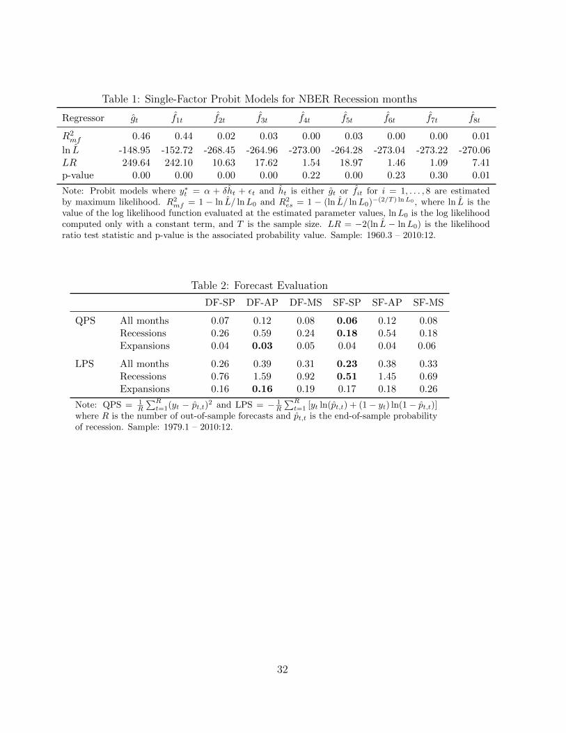
Table 1: Single-Factor Probit Models for NBER Recession months

Regressor gt f1t f2t f3t f4t f5t f6t f7t f8t

R2mf 0.46 0.44 0.02 0.03 0.00 0.03 0.00 0.00 0.01

ln L -148.95 -152.72 -268.45 -264.96 -273.00 -264.28 -273.04 -273.22 -270.06LR 249.64 242.10 10.63 17.62 1.54 18.97 1.46 1.09 7.41p-value 0.00 0.00 0.00 0.00 0.22 0.00 0.23 0.30 0.01

Note: Probit models where y∗t = α + δht + εt and ht is either gt or fit for i = 1, . . . , 8 are estimatedby maximum likelihood. R2

mf = 1 − ln L/ lnL0 and R2es = 1 − (ln L/ lnL0)−(2/T ) lnL0 , where ln L is the

value of the log likelihood function evaluated at the estimated parameter values, lnL0 is the log likelihoodcomputed only with a constant term, and T is the sample size. LR = −2(ln L − lnL0) is the likelihoodratio test statistic and p-value is the associated probability value. Sample: 1960.3 – 2010:12.

Table 2: Forecast Evaluation

DF-SP DF-AP DF-MS SF-SP SF-AP SF-MS

QPS All months 0.07 0.12 0.08 0.06 0.12 0.08Recessions 0.26 0.59 0.24 0.18 0.54 0.18Expansions 0.04 0.03 0.05 0.04 0.04 0.06

LPS All months 0.26 0.39 0.31 0.23 0.38 0.33Recessions 0.76 1.59 0.92 0.51 1.45 0.69Expansions 0.16 0.16 0.19 0.17 0.18 0.26

Note: QPS = 1R

∑Rt=1(yt − pt,t)2 and LPS = − 1

R

∑Rt=1 [yt ln(pt,t) + (1− yt) ln(1− pt,t)]

where R is the number of out-of-sample forecasts and pt,t is the end-of-sample probabilityof recession. Sample: 1979.1 – 2010:12.

32

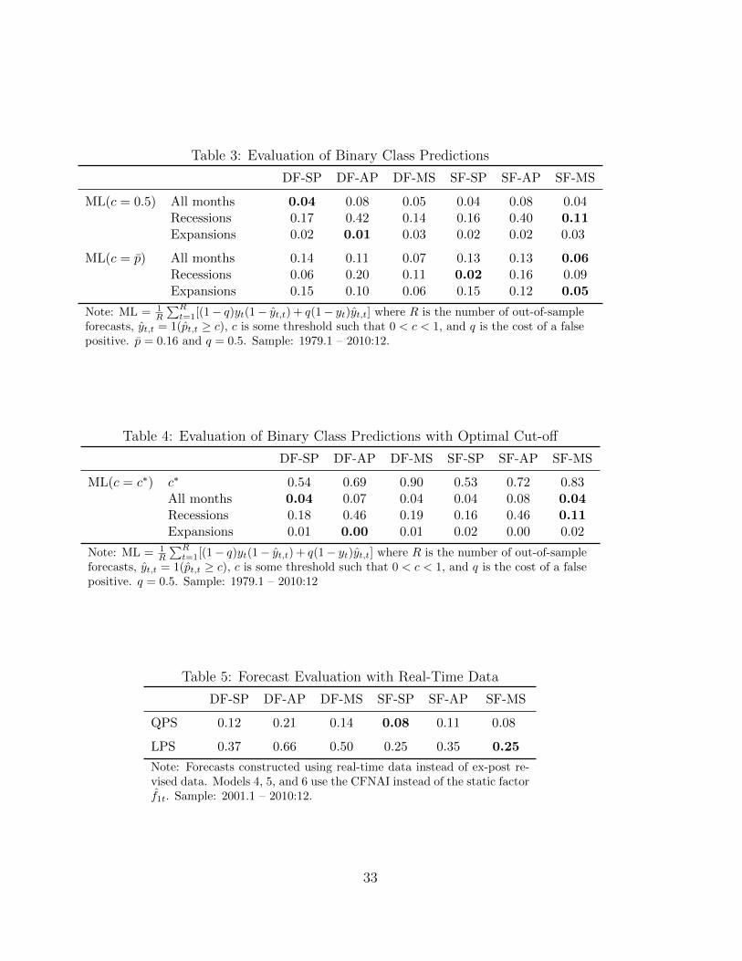
Table 3: Evaluation of Binary Class Predictions


ML(c = 0.5) All months 0.04 0.08 0.05 0.04 0.08 0.04Recessions 0.17 0.42 0.14 0.16 0.40 0.11Expansions 0.02 0.01 0.03 0.02 0.02 0.03

ML(c = p) All months 0.14 0.11 0.07 0.13 0.13 0.06Recessions 0.06 0.20 0.11 0.02 0.16 0.09Expansions 0.15 0.10 0.06 0.15 0.12 0.05

Note: ML = 1R

∑Rt=1[(1− q)yt(1− yt,t) + q(1− yt)yt,t] where R is the number of out-of-sample

forecasts, yt,t = 1(pt,t ≥ c), c is some threshold such that 0 < c < 1, and q is the cost of a falsepositive. p = 0.16 and q = 0.5. Sample: 1979.1 – 2010:12.

Table 4: Evaluation of Binary Class Predictions with Optimal Cut-off


ML(c = c∗) c∗ 0.54 0.69 0.90 0.53 0.72 0.83All months 0.04 0.07 0.04 0.04 0.08 0.04Recessions 0.18 0.46 0.19 0.16 0.46 0.11Expansions 0.01 0.00 0.01 0.02 0.00 0.02

Note: ML = 1R

∑Rt=1[(1− q)yt(1− yt,t) + q(1− yt)yt,t] where R is the number of out-of-sample

forecasts, yt,t = 1(pt,t ≥ c), c is some threshold such that 0 < c < 1, and q is the cost of a falsepositive. q = 0.5. Sample: 1979.1 – 2010:12

Table 5: Forecast Evaluation with Real-Time Data


QPS 0.12 0.21 0.14 0.08 0.11 0.08

LPS 0.37 0.66 0.50 0.25 0.35 0.25

Note: Forecasts constructed using real-time data instead of ex-post re-vised data. Models 4, 5, and 6 use the CFNAI instead of the static factorf1t. Sample: 2001.1 – 2010:12.

33

←Dynamic Factor

1960 1965 1970 1975 1980 1985 1990 1995 2000 2005 2010−8

−6

−4

−2

0

2

4

Figure 1: Dynamic factor (gt) and capacity utilization. Standardized units are re-ported. Shaded areas denote NBER recession months.

←First PC Factor

1960 1965 1970 1975 1980 1985 1990 1995 2000 2005 2010−6

−5

−4

−3

−2

−1

0

1

2

3

Figure 2: First principal components factor (f1t) and capacity utilization. Standardizedunits are reported. Shaded areas denote NBER recession months.

34

1960 1965 1970 1975 1980 1985 1990 1995 2000 2005 2010

0

0.2

0.4

0.6

0.8

1

Figure 3: In-sample probabilities of recession from the single-factor probit model usinggt as predictor. Shaded areas denote NBER recession months.

1960 1965 1970 1975 1980 1985 1990 1995 2000 2005 2010

0

0.2

0.4

0.6

0.8

1

Figure 4: In-sample probabilities of recession from the single-factor probit model usingf1t as predictor. Shaded areas denote NBER recession months.

35

(1) DF−SP

1980 1985 1990 1995 2000 2005 20100

0.2

0.4

0.6

0.8

1

(2) DF−AP

1980 1985 1990 1995 2000 2005 20100

0.2

0.4

0.6

0.8

1

(3) DF−MS

1980 1985 1990 1995 2000 2005 20100

0.2

0.4

0.6

0.8

1

(4) SF−SP

1980 1985 1990 1995 2000 2005 20100

0.2

0.4

0.6

0.8

1

(5) SF−AP

1980 1985 1990 1995 2000 2005 20100

0.2

0.4

0.6

0.8

1

(6) SF−MS

1980 1985 1990 1995 2000 2005 20100

0.2

0.4

0.6

0.8

1

Figure 5: End-of-sample probabilities of recession (pt,t) for the period 1979:1 – 2010:12.Shaded areas denote NBER recession months.

36

(1) DF−SP

1980 1985 1990 1995 2000 2005 20100

0.2

0.4

0.6

0.8

1

(2) DF−AP

1980 1985 1990 1995 2000 2005 20100

0.2

0.4

0.6

0.8

1

(3) DF−MS

1980 1985 1990 1995 2000 2005 20100

0.2

0.4

0.6

0.8

1

(4) SF−SP

1980 1985 1990 1995 2000 2005 20100

0.2

0.4

0.6

0.8

1

(5) SF−AP

1980 1985 1990 1995 2000 2005 20100

0.2

0.4

0.6

0.8

1

(6) SF−MS

1980 1985 1990 1995 2000 2005 20100

0.2

0.4

0.6

0.8

1

Figure 6: Probabilities of recession (paths) for the period 1979:1 – 2010:12. Shadedareas denote NBER recession months.

37

Cut−off = 0.50

q

0 0.2 0.4 0.6 0.8 10

0.1

0.2

Cut−off = 0.16

q

0 0.2 0.4 0.6 0.8 10

0.1

0.2

Figure 7: ML for different values of q. Solid lines represent standard probit models.Dotted lines represent autoregressive probit models. Dashed lines represent Markov-switching models. Blue (dark) lines represents models using gt. Gray (light) linesrepresents models using f1t.

38

Documents

Dating U.S. Business Cycles with Macro Factorssfossati/files/pdfs/factor_probit.pdf · Dating US Business Cycles with Macro Factors Sebastian Fossati University of Alberta This version: